Condensation vs Ordering: From the Spherical Models to BEC in the Canonical and Grand Canonical Ensemble

Abstract

In this paper we take a fresh look at the long standing issue of the nature of macroscopic density fluctuations in the grand canonical treatment of the Bose-Einstein condensation (BEC). Exploiting the close analogy between the spherical and mean-spherical models of magnetism with the canonical and grand canonical treatment of the ideal Bose gas, we show that BEC stands for different phenomena in the two ensembles: an ordering transition of the type familiar from ferromagnetism in the canonical ensemble and condensation of fluctuations, i.e. growth of macroscopic fluctuations in a single degree of freedom, without ordering, in the grand canonical case. We further clarify that this is a manifestation of nonequivalence of the ensembles, due to the existence of long range correlations in the grand canonical one. Our results shed new light on the recent experimental realization of BEC in a photon gas, suggesting that the observed BEC when prepared under grand canonical conditions is an instance of condensation of fluctuations.

I Introduction

In general statistical ensembles are constructed to be equivalent in the thermodynamic limit, but there are exceptions to this rule. This paper deals with phenomena arising when this equivalence breaks down. Pairs of conjugate ensembles are obtained by controlling the system either by fixing the value of some extensive quantity, through appropriate isolating walls, or by putting it in contact with a reservoir of that same quantity. A familiar example, which will be of central interest in the following, is that of the canonical and grand canonical pair resulting from fixing either the density of particles or the chemical potential, while keeping the system thermalized.

Basically, equivalence holds in situations in which correlations are short ranged. Then, the central limit theorem guarantees that fluctuations of extensive quantities become negligible in the thermodynamic limit, so that it doesn’t matter whether the system is controlled by enforcing a rigid constraint or through the contact with a reservoir Huang ; Pathria ; Puglisi . By the same token lack of equivalence is to be expected when correlations are long ranged. This is a more rare occurrence, but very interesting since new physics obtains by switching from one ensemble to the other within a conjugate pair. Best known and recently much studied is the case of systems with long-range interactions Campa .

There is one instance of nonequivalence which stands apart: The one which materializes as an ideal Bose gas (IBG) is driven through the Bose-Einstein condensation (BEC). In the canonical ensemble (CE) fluctuations of the condensate behave normally while in the grand canonical ensemble (GCE) do persist even in the thermodynamic limit  Pathria ; Ziff . Although this is an exact result, it is somewhat puzzling because, dealing with an ideal gas, it is not at all obvious where the long range correlations responsible of the nonequivalence could come from. An unbiased attitude ought to advise to take the facts at face value and to inquiry on possible different mechanisms underlying BEC in the two ensembles. Instead, due to a widespread aversion to macroscopic fluctuations of an extensive quantity, which are not suppressed by lowering the temperature, the GCE result has been variously regarded as unacceptable Holthaus , unphysical Fujiwara ; Ziff ; Stringari ; Scully or even wrong Yukalov and is commonly referred to as the grand canonical catastrophe.

The need to reconsider afresh this matter has been prompted by the recent observation of BEC in the lab Klaers ; Schmitt in a gas of photons under grand canonical conditions, which has changed the outlook by producing evidence for the existence of the macroscopic fluctuations of the condensate. Therefore, after reckoning with the absence of any catastrophe, the challenge is to uncover the mechanism responsible of the nonequivalence. Due to the fundamental character of the question posed, we shall leave the experiment in the background and we shall explore the basic issues in the simplest possible context of the uniform IBG in a box of volume $V$, aiming primarily to outline the conceptual framework needed to approach this interesting and multifaceted problem.

II The Problem

At the phenomenological level the mechanism of BEC appears to be the same in the CE and in the GCE. Denoting by $d$, $d^{*}$ and $d_{0}$ the total density, the density in the excited states and the density in the ground state, respectively, from the obvious identity $d=d^{*}+d_{0}$ follows the sum rule which must be satisfied by the average quantities irrespective of the choice of the ensemble

$$\rho=\langle d^{*}\rangle+\langle d_{0}\rangle,$$ (1)

where $\rho$ stands for $\langle d\rangle$ and the brackets for the average over either ensemble. The condensate density $\langle d_{0}\rangle$ is called the BEC order parameter. Now, for space dimensionality $d>2$ and in the thermodynamic limit, $\langle d^{*}\rangle$ is superiorly bounded by a finite critical value $\rho_{c}$ Huang ; Pathria . Consequently, keeping $T$ fixed and using $\rho$ as control parameter, from Eq. (1) immediately follows the density-driven BEC

$$\langle d_{0}\rangle=\left\{\begin{array}[]{ll}0,\;\;$for$\;\;\rho\leq\rho_{c},\\ \rho-\rho_{c},\;\;$for$\;\;\rho>\rho_{c},\end{array}\right.$$ (2)

which, we emphasize, holds irrespective of the ensemble. Thus, as far as $\langle d_{0}\rangle$ is concerned, CE and GCE are equivalent. However, a striking difference between the two emerges when the fluctuations of $d_{0}$ are considered, since in the condensed phase, as previously anticipated, one has Ziff

$$\left\langle\left(d_{0}-\langle d_{0}\rangle\right)^{2}\right\rangle=\left\{\begin{array}[]{ll}0,\;\;$in the CE$,\\ \langle d_{0}\rangle^{2}\;\;$in the GCE$,\end{array}\right.$$ (3)

i.e. normal behavior in the CE and macroscopic fluctuations in the GCE.

The crux of the matter is that at this level of observation no insight can be obtained as to the why fluctuations ought to behave so differently in the two ensembles. The point of view that we propose in this paper is that the picture is rationalized by shifting the description to the finer and underlying level of the field-theoretic microscopic degrees of freedom, which however are not directly observable. In order to clarify the interplay of the different levels of description, in the next paragraph we shall exploit the analogy with magnetic systems, where a quite similar and well understood situation arises.

III Spherical and Mean-Spherical Model

The IBG in the CE and in the GCE is well known KT ; Kac2 ; Cannon to be closely related to the spherical and the mean-spherical models of magnetism. Let ${\cal H}(\boldsymbol{\varphi})=\int_{V}d\vec{r}\,\varphi(\vec{r})\left(-\frac{1}{2}\nabla^{2}\right)\varphi(\vec{r})$ be the energy function of a classical scalar paramagnet Ma in the volume $V$, where $\boldsymbol{\varphi}$ stands for a configuration of the local unbounded spin variable $\varphi(\vec{r})$. Due to its bilinear character the above Hamiltonian can be diagonalized by Fourier transform ${\cal H}=\frac{1}{V}\sum_{\vec{k}}k^{2}|\varphi_{\vec{k}}|^{2}$. In the spherical model (SM) of Berlin and Kac BK a coupling among the modes is induced by the imposition of an overall constraint on the square magnetization ${\cal S}(\boldsymbol{\varphi})=\int_{V}d\vec{r}\,\varphi^{2}(\vec{r})=\frac{1}{V}\sum_{\vec{k}}|\varphi_{\vec{k}}|^{2}$. Then, in thermal equilibrium the statistical ensemble reads

$$P_{\textrm{SM}}(\boldsymbol{\varphi}|\sigma)=\frac{1}{Z_{\textrm{SM}}}e^{-\beta{\cal H}(\boldsymbol{\varphi})}\,\delta\left(\mathit{s}(\boldsymbol{\varphi})-\sigma\right),$$ (4)

where $Z_{\textrm{SM}}$ is the partition function, $\mathit{s}(\boldsymbol{\varphi})=\frac{1}{V}{\cal S}(\boldsymbol{\varphi})$ the square magnetization density and $\sigma$ a positive number, which usually is set $\sigma=1$, but here will be kept free to vary as a control parameter. In the mean-spherical model (MSM) LW ; KT the constraint is imposed in the mean: An ${\cal S}$-dependent exponential bias is introduced in place of the $\delta$ function

$$P_{\textrm{MSM}}(\boldsymbol{\varphi}|\sigma)=\frac{1}{Z_{\textrm{MSM}}}e^{-\beta[{\cal H}(\boldsymbol{\varphi})+\frac{\kappa}{2}{\cal S}(\boldsymbol{\varphi})]},$$ (5)

and the intensive parameter $\kappa$ conjugate to ${\cal S}$ must be adjusted so as to satisfy the requirement

$$\langle\mathit{s}(\boldsymbol{\varphi})\rangle_{\textrm{MSM}}=\sigma.$$ (6)

Although it is the common usage to refer to these as models, it should be clear from Eqs. (4) and (5) that we are dealing with two conjugate ensembles, distinguished by conserving or letting to fluctuate the density $\mathit{s}$. Separating the excitations from the ground state contribution $\mathit{s}=\mathit{s}^{*}+\mathit{s}_{0}$, where $\mathit{s}^{*}=\frac{1}{V^{2}}\sum_{\vec{k}\neq 0}|\varphi_{\vec{k}}|^{2}$ and $\mathit{s}_{0}=\frac{1}{V^{2}}\varphi_{0}^{2}$, taking the average and using the constraint $\langle\mathit{s}\rangle=\sigma$, independently from the choice of the model there follows the sum rule analogous to Eq. (1)

$$\sigma=\langle\mathit{s}^{*}\rangle+\langle\mathit{s}_{0}\rangle.$$ (7)

Therefore, the variables $\mathit{s},\mathit{s}^{*},\mathit{s}_{0}$ and $\sigma$ do correspond to the IBG ones $d,d^{*},d_{0}$ and $\rho$, with the important difference that in the present context these are composite variables, built in terms of the microscopic set of the magnetization components $[\varphi_{\vec{k}}]$. Furthermore, also in this case for $d>2$ and in the thermodynamic limit the excitation contribution $\langle\mathit{s}^{*}\rangle$ is superiorly bounded by a finite critical value $\sigma_{c}$, see Appendices A and B for details. Hence, keeping $T$ fixed and varying $\sigma$, from Eq. (7) there follows

$$\langle\mathit{s}_{0}\rangle=\left\{\begin{array}[]{ll}0,\;\;$for$\;\;\sigma\leq\sigma_{c},\\ \sigma-\sigma_{c},\;\;$for$\;\;\sigma>\sigma_{c},\end{array}\right.$$ (8)

showing that $\langle\mathit{s}_{0}\rangle$ behaves like the BEC order parameter and that, as far as $\langle\mathit{s}_{0}\rangle$ is concerned, the two models are equivalent.

However, at the microscopic level a different scenario opens up, since there is no unique way to form a finite expectation $\langle\mathit{s}_{0}\rangle$. Let us introduce the probability that $\mathit{s}$ takes the value $\sigma^{\prime}$ in the MSM, given by $K_{\textrm{MSM}}(\sigma^{\prime}|\sigma)=\int d\boldsymbol{\varphi}\,P_{\textrm{MSM}}(\boldsymbol{\varphi}|\sigma)\delta\left(\mathit{s}(\boldsymbol{\varphi})-\sigma^{\prime}\right)$. Then, just as a consequence of definitions, the distributions  (4) and (5) are related by

$$P_{\textrm{MSM}}(\boldsymbol{\varphi}|\sigma)=\int_{0}^{\infty}d\sigma^{\prime}\,P_{\textrm{SM}}(\boldsymbol{\varphi}|\sigma^{\prime})K_{\textrm{MSM}}(\sigma^{\prime}|\sigma).$$ (9)

The kernel has been worked out by Kac and Thompson KT , obtaining $K_{\textrm{MSM}}(\sigma^{\prime}|\sigma)=\delta(\sigma^{\prime}-\sigma)$ for $\sigma<\sigma_{c}$, which implies that the two distributions coincide and, therefore, that the two models are equivalent below $\sigma_{c}$. Conversely, when $\sigma$ is above $\sigma_{c}$ the kernel vanishes for $\sigma^{\prime}<\sigma_{c}$, while for $\sigma^{\prime}>\sigma_{c}$ is of the spread out form

$$K_{\textrm{MSM}}(\sigma^{\prime}|\sigma)=\frac{e^{-\frac{\sigma^{\prime}-\sigma_{c}}{2(\sigma-\sigma_{c})}}}{\sqrt{2\pi(\sigma^{\prime}-\sigma_{c})(\sigma-\sigma_{c})}},$$ (10)

revealing nonequivalence. In the following we shall restrict to the $\sigma>\sigma_{c}$ domain, where nontrivial behavior is expected. Integrating out the $\vec{k}\neq 0$ modes from Eq. (9), an identical relation between the marginal probabilities of $\psi_{0}=\frac{1}{V}\varphi_{0}$ is obtained. In the left hand side there appears the Gaussian distribution $P_{\textrm{MSM}}(\psi_{0}|\sigma)\propto\exp\{-\beta\kappa V\psi_{0}^{2}/2\}$, as it can be verified by inspection from Eq. (5), since $P_{\textrm{MSM}}(\boldsymbol{\varphi}|\sigma)$ factorizes in Fourier space. From this follows $\langle\mathit{s}_{0}\rangle=(\beta\kappa V)^{-1}$. So, from the second line of Eq. (8) we get

$$\kappa=1/[\beta V(\sigma-\sigma_{c})],$$ (11)

which implies

$$P_{\textrm{MSM}}(\psi_{0}|\sigma)=\frac{e^{-\frac{1}{2(\sigma-\sigma_{c})}\psi_{0}^{2}}}{\sqrt{2\pi(\sigma-\sigma_{c})}}.$$ (12)

Hence, plugging in the explicit expression of $K_{\textrm{MSM}}(\sigma^{\prime}|\sigma)$ it is not difficult to verify that Eq. (9) is satisfied by the ansatz

$$P_{\textrm{SM}}(\psi_{0}|\sigma)=\frac{1}{2}[\delta(\psi_{0}-m_{-})+\delta(\psi_{0}-m_{+})],$$ (13)

where $m_{\pm}=\pm\sqrt{\sigma-\sigma_{c}}$ is the spontaneous magnetization density which would be obtained, for instance, by switching off an external magnetic field BK ; KT . Thus, we have two quite different distributions, as it is clearly illustrated by the plots in Fig. 1.

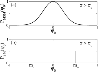
Figure 1: Distributions of $\psi_{0}$ in the MSM model (a) and in the SM model (b) for $\sigma>\sigma_{c}$. The spikes in the bottom panel stand for $\delta$ functions.

We are now in the position to draw some conclusions. The BEC-like order parameter $\langle\mathit{s}_{0}\rangle$ can be computed microscopically as the average composite variable $\langle\psi_{0}^{2}\rangle$. Then, it is straightforward to check from Eqs. (12) and (13) that Eq. (8) is satisfied in both cases. However, it is enough to take a look at Fig. 1 to realize that the numerically identical result $\langle\psi_{0}^{2}\rangle=(\sigma-\sigma_{c})$ for $\sigma>\sigma_{c}$ in the two models stands for two different phenomena. The double peaked distribution of the SM case is the familiar one for a ferromagnet in the magnetized phase, each peak being associated to a pure state and with the up-down symmetry of the model spontaneously broken. Namely, the distribution is the even mixture of these two pure states. This means that in the SM the BEC-like transition observed at the level of $\langle\mathit{s}_{0}\rangle$ is the manifestation of an underlying ordering transition, and that the BEC order parameter is the square of the spontaneous magnetization, i.e. $\langle\psi_{0}^{2}\rangle=m_{\pm}^{2}$. By contrast, in the MSM case we have the opposite situation, since $\langle\psi_{0}^{2}\rangle$ is the variance of a broad Gaussian distribution centered on the origin. Therefore there is no ordering, no breaking of the symmetry. In this case the BEC-like transition undergone by $\langle\mathit{s}_{0}\rangle$ is the manifestation of the microscopic variable $\psi_{0}$ developing finite fluctuations. The reason for this can be grasped intuitively. In the SM, due to the sharp constraint, there is enough nonlinearity to produce ordering. In the MSM framework this cannot be achieved, since the statistics are Gaussian. Then, the only mean to build up the finite value of $\langle\mathit{s}_{0}\rangle$ needed to saturate the sum rule (7) above $\sigma_{c}$ is by growing fluctuations in the single degree of freedom $\psi_{0}$. Elsewhere EPL ; CCZ ; Zannetti ; Merhav ; Marsili , this type of transition, characterized by the fluctuations of an extensive quantity condensing into one microscopic component, has been referred to as condensation of fluctuations. The phenomenological picture is completed by the fluctuations of $\mathit{s}_{0}$ itself which, as it follows easily from Eqs. (12) and (13), are given by

$$\left\langle\left(\mathit{s}_{0}-\langle\mathit{s}_{0}\rangle\right)^{2}\right\rangle=\left\{\begin{array}[]{ll}0,\;\;$in the SM$,\\ 2\langle\mathit{s}_{0}\rangle^{2},\;\;$in the MSM$.\end{array}\right.$$ (14)

Comparing this with Eq. (3), the analogy is evident. However, now no catastrophical behavior can be envisaged, because the fluctuations of $\mathit{s}_{0}$ are trivially a consequence of the different microscopic statistics in the two models.

Having analysed how the nonequivalence unfolds, the remaining task is to clarify where it does to originate from, which ultimately must be in the presence of long range correlations. The explanation is that in the MSM the parameter $\kappa$ is related to the correlation length $\xi$ by $\kappa=\xi^{-2}$ Ma and from Eq. (11) we see that in the thermodynamic limit $\kappa$ vanishes like $1/V$ when $\sigma$ is fixed above $\sigma_{c}$. Therefore, in the entire condensed phase the MSM is critical, while the SM is not. Hence, the lack of equivalence. We emphasize that the onset of these critical correlations in the MSM is the unifying thread behind the BEC-like transition accompanied by macroscopic fluctuations of $\mathit{s}_{0}$.

IV Back to the IBG

We may now go back to the main topic of the IBG with the advantage of hindsight, since we know what to look for: The microscopic variables underlying the phenomenological level, in terms of which we expect to expose both the different mechanisms of BEC in the CE and GCE and the nonequivalence cause. This is accomplished by introducing the creation and destruction operators and by using the representation of the density matrix in the associated coherent state basis. Let us first diagonalize the energy and number operators by Fourier transform ${\cal H}=\sum_{\vec{k}}\epsilon_{\vec{k}}a_{\vec{k}}^{\dagger}a_{\vec{k}}$ and ${\cal N}=\sum_{\vec{k}}a_{\vec{k}}^{\dagger}a_{\vec{k}}$, where $\epsilon_{\vec{k}}$ is the single particle energy. In the Glauber-Sudarshan P-representation Glauber ; Sudarshan the density matrix is given by $D(\rho)=\int d^{2}\boldsymbol{\alpha}\,P(\boldsymbol{\alpha}|\rho)|\boldsymbol{\alpha}\rangle\langle\boldsymbol{\alpha}|$, where $|\boldsymbol{\alpha}\rangle$ are product states $\prod_{\vec{k}}|\alpha_{\vec{k}}\rangle$ and the $\vec{k}$-mode factor $|\alpha_{\vec{k}}\rangle$ is the eigenvector of the annihilation operator $a_{\vec{k}}|\alpha_{\vec{k}}\rangle=\alpha_{\vec{k}}|\alpha_{\vec{k}}\rangle$ with complex eigenvalue $\alpha_{\vec{k}}$. Then, in the GCE the weight function reads Glauber

$$P_{\textrm{GCE}}(\boldsymbol{\alpha}|\rho)=\prod_{\vec{k}}\frac{1}{\pi\langle n_{\vec{k}}\rangle}\exp\left\{-\frac{|\alpha_{\vec{k}}|^{2}}{\langle n_{\vec{k}}\rangle}\right\},$$ (15)

where $\langle n_{\vec{k}}\rangle=[e^{\beta(\epsilon_{k}-\mu)}-1]^{-1}$ is the usual Bose average occupation number of the state $|\vec{k}\rangle$ Huang and $\mu$ stands for the chemical potential. Using the identity $\langle|\alpha_{\vec{k}}|^{2}\rangle=\langle n_{\vec{k}}\rangle$, which easily follows from Eq. (15), the equation fixing $\mu$ for the given value of $\rho$ reads $\frac{1}{V}\sum_{\vec{k}}\langle|\alpha_{\vec{k}}|^{2}\rangle=\rho$. Since this is nothing but Eq. (1), we may write $d=\frac{1}{V}\sum_{\vec{k}}|\alpha_{\vec{k}}|^{2}$ and, consequently, $d_{0}=|\eta_{0}|^{2}$, after setting $\eta_{0}=\frac{1}{\sqrt{V}}\alpha_{0}$. This allows to identify $[\alpha_{\vec{k}}]$ with the sought for set of microscopic variables analogous to $[\varphi_{\vec{k}}]$. Following the magnetic example, we must focus on the statistics of the zero component, keeping in mind however that now is a complex quantity $\eta_{0}=|\eta_{0}|e^{i\theta}$. The starting point is the relation between ensembles analogous to Eq. (9) (see Appendices C and D)

$$P_{\textrm{GCE}}(\boldsymbol{\alpha}|\rho)=\int_{0}^{\infty}d\rho^{\prime}\,P_{\textrm{CE}}(\boldsymbol{\alpha}|\rho^{\prime})K_{\textrm{GCE}}(\rho^{\prime}|\rho),$$ (16)

where $K_{\textrm{GCE}}(\rho^{\prime}|\rho)$ is the probability in the CGE that the density takes the value $\rho^{\prime}$. This is known as the Kac function Ziff , whose form is similar to that of Eq. (10). Namely, $K_{\textrm{GCE}}(\rho^{\prime}|\rho)=\delta(\rho^{\prime}-\rho)$ for $\rho<\rho_{c}$, while when $\rho$ is above $\rho_{c}$ it vanishes for $\rho^{\prime}<\rho_{c}$ and is given by

$$K_{\textrm{GCE}}(\rho^{\prime}|\rho)=\frac{e^{-\frac{\rho^{\prime}-\rho_{c}}{\rho-\rho_{c}}}}{\rho-\rho_{c}},\quad\text{for}\quad\rho^{\prime}>\rho_{c}.$$ (17)

The relation between the $\eta_{0}$ marginal distributions is then obtained by integrating out the $\vec{k}\neq 0$ modes $P_{\textrm{GCE}}(\eta_{0}|\rho)=\int_{0}^{\infty}d\rho^{\prime}\,P_{\textrm{CE}}(\eta_{0}|\rho^{\prime})\,K_{\textrm{GCE}}(\rho^{\prime}|\rho)$. Inserting in the left hand side the contribution from the first factor of Eq. (15)

$$P_{\textrm{GCE}}(\eta_{0}|\rho)=\frac{V}{\pi\langle n_{0}\rangle}\exp\left\{-\frac{V|\eta_{0}|^{2}}{\langle n_{0}\rangle}\right\},$$ (18)

and substituting for $K_{\textrm{GCE}}(\rho^{\prime}|\rho)$ the above expression, the equation is solved by the ansatz

$$P_{\textrm{CE}}(\eta_{0}|\rho)=\frac{1}{\pi}\,\delta(|\eta_{0}|^{2}-(\rho-\rho_{c})).$$ (19)

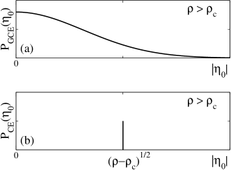
Figure 2: Distributions of $|\eta_{0}|$ in the GCE (a) and in the CE (b) for $\rho>\rho_{c}$. The spike in the bottom panel stands for the $\delta$ function distribution.

From the plot of the two distributions (18) and (19) in Fig. 2, we see by inspection that we are confronted with a situation qualitatively similar to the one in the magnetic case. In both ensembles $|\eta_{0}|$ develops a nonobservable finite expectation value

$$\langle|\eta_{0}|\rangle=\left\{\begin{array}[]{ll}\sqrt{\rho-\rho_{c}},\;\;$CE$,\\ \frac{1}{2}\sqrt{\pi(\rho-\rho_{c})},\;\;$GCE$.\end{array}\right.$$ (20)

The observable BEC order parameter exhibits the same numerical value as in Eq. (2)

$$\langle d_{0}\rangle=\langle|\eta_{0}|^{2}\rangle=\left\{\begin{array}[]{ll}(\rho-\rho_{c}),\;\;$CE$,\\ (\rho-\rho_{c}),\;\;$GCE$,\end{array}\right.$$ (21)

which is achieved through fluctuations in the GCE and without fluctuations in the CE

$$\left\langle\left(|\eta_{0}|-\langle|\eta_{0}|\rangle\right)^{2}\right\rangle=\left\{\begin{array}[]{ll}0,\;\;$CE$,\\ (1-\pi/4)(\rho-\rho_{c}),\;\;$GCE$.\end{array}\right.$$ (22)

This means that the sum rule (1) in the CE is saturated by fixing the modulus to the precise finite value $|\eta_{0}|=\sqrt{\rho-\rho_{c}}$. Because of this freezing of $|\eta_{0}|$, BEC in the CE fits into the scheme of an ordering transition akin to the ferromagnetic transition in the SM. Conversely, BEC in the GCE does not take place through ordering. Rather, the saturation of the sum rule is achieved by growing the macroscopic fluctuations of $|\eta_{0}|$, as Eq. (22) shows. Therefore, in this case BEC fits into the scheme of the condensation transition. Ordering is ruled out because the width of the probability distribution persists in the thermodynamic limit. Moreover, assuming $\epsilon_{k}\sim k^{\alpha}$, where the power $\alpha$ depends on the dispersion relation, for small $k$ and small $\mu$ we may approximate $\langle n_{\vec{k}}\rangle^{-1}\simeq\beta[k^{\alpha}-\mu]$ and inserting this into Eq. (15) we have that the chemical potential, like $\kappa$ in the preceding case, is connected to the correlation length by $-\mu=\xi^{-\alpha}$. Since the formation of the condensed phase in the GCE requires $\mu$ to vanish in the thermodynamic limit Huang , we have that the condensed phase is critical throughout in the GCE but not in the CE. This explains the origin of nonequivalence which, as in the magnetic case, is not revealed by the BEC order parameter but emerges only at the level of the higher cumulant

$$\left\langle\left(|\eta_{0}|^{2}-\langle|\eta_{0}|^{2}\rangle\right)^{2}\right\rangle=\left\{\begin{array}[]{ll}(\rho-\rho_{c})^{2},\;\;$GCE$,\\ 0,\;\;$CE$.\end{array}\right.$$ (23)

Hence, the phenomenological result of Eq. (3), rather than being pathological, is now accounted for as a byproduct of the critical correlations in the GCE.

V Summary

In this paper we have investigated the differences arising when BEC in a homogeneous IBG is treated in the CE and in the GCE. The analysis has been carried out by taking advantage of the close analogy with the the spherical and mean spherical models of magnetism. The problem is of particular interest because the ensemble nonequivalence issue encroaches the fundamental question of the nature of BEC. We have shown that ordering takes place in the CE, while condensation takes place in the GCE, whose prominent manifestation are the macroscopic fluctuations of the condensate. Therefore, we suggest that the recent experimental realization of BEC in a gas of photons Klaers ; Schmitt ; Klaers2 ought to be regarded as qualitatively different from other experimental instances of BEC, such as those with cold atoms, precisely because the grand canonical conditions lead to BEC as condensation of fluctuations. Moreover, by retracing the origin of nonequivalence to the onset of critical correlations in the condensed phase of the GCE, we have pointed out that the observable phenomenology follows as a consequence. So, knowledge of the existence of these correlations could possibly serve as a useful guide in the planning of future experiments. As a final remark, notice that the above analysis has involved the modulus, but not the phase of $\eta_{0}$. This means that the distinction between ordering and condensation is decoupled from the issue of the breaking of the gauge symmetry. This is a separate and important problem which will be the object of future work.

Appendix A Spherical and Mean Spherical Model

Let ${\boldsymbol{\varphi}}$ be a configuration of the magnetization field $\varphi(\vec{r})\in(-\infty,+\infty)$ over an hypercube ${\vec{r}}\in V\subset\mathbb{R}^{d}$ of side $L$, whose energy is given by

$${\cal H}(\boldsymbol{\varphi})=\int_{V}d\vec{r}\,\varphi(\vec{r})\left(-\frac{1}{2}\nabla^{2}\right)\varphi(\vec{r}).$$ (24)

Ensembles, or models, are defined by thermalizing the system and specifying conditions imposed on the overall square magnetization

$${\cal S}(\boldsymbol{\varphi})=\int_{V}d{\vec{r}}\,\varphi^{2}({\vec{r}}).$$ (25)

The spherical model (SM) of Berlin and Kac BK , which corresponds to the ensemble canonical with respect to ${\cal S}(\boldsymbol{\varphi})$, is obtained by imposing a sharp constraint on the sqaure magnetization density

$$\mathit{s}(\boldsymbol{\varphi})=\sigma,$$ (26)

where $\mathit{s}(\boldsymbol{\varphi})=\frac{1}{V}{\cal S}(\boldsymbol{\varphi})$ and $\sigma$ is a positive number. This leads to the probability distribution

$$P_{\textrm{SM}}({\boldsymbol{\varphi}})=\frac{1}{Z_{\textrm{SM}}}\,e^{-\beta{\cal H}({\boldsymbol{\varphi}})}\,\delta\left(\mathit{s}(\boldsymbol{\varphi})-\sigma\right),$$ (27)

with the partition function

$$Z_{\textrm{SM}}=\int{\cal D}{\boldsymbol{\varphi}}\,e^{-\beta{\cal H}({\boldsymbol{\varphi}})}\,\delta\left(\mathit{s}(\boldsymbol{\varphi})-\sigma\right).$$ (28)

The mean spherical model (MSM) of Lewis and Wannier LW , which corresponds to the ensemble grand canonical with respect to ${\cal S}(\boldsymbol{\varphi})$, is defined by

$$P_{\textrm{MSM}}({\boldsymbol{\varphi}}|\sigma)=\frac{1}{Z_{\textrm{MSM}}}\,\exp\left\{-\beta[{\cal H}({\boldsymbol{\varphi}})+\frac{\kappa}{2}\,{\cal S}(\boldsymbol{\varphi})]\right\},$$ (29)

with the partition function

$$Z_{\textrm{MSM}}=\int{\cal D}{\boldsymbol{\varphi}}\,\exp\left\{-\beta[{\cal H}({\boldsymbol{\varphi}})+\frac{\kappa}{2}\,{\cal S}(\boldsymbol{\varphi})]\right\},$$ (30)

and where the parameter $\kappa$ is determined self-consistently by imposing the constraint (26) on average

$$\langle\mathit{s}(\boldsymbol{\varphi})\rangle_{\textrm{MSM}}=\sigma,$$ (31)

as it is explained in the next section. Notice that in both models $\beta$ and $\sigma$ are control parameters.

Appendix B Solution of the mean spherical model

Imposing periodic boundary conditions and postulating the existence of a microscopic length $a_{0}$, the allowed wave vectors of the Fourier components

$$\varphi_{\vec{k}}=\int_{V}d\vec{r}\,\varphi(\vec{r})\,e^{i\vec{k}\cdot\vec{r}}$$ (32)

are given by

$$\vec{k}=\frac{2\pi}{L}\vec{n},\;\;\;n_{i}=0,\pm 1,\pm 2,...,\pm N_{\rm max},$$ (33)

where $N_{\rm max}=L/a_{0}$ supposedly is an integer. The inverse transform reads

$$\varphi(\vec{r})=\frac{1}{V}\sum_{\vec{k}}\varphi_{\vec{k}}\,e^{-i\vec{k}\cdot\vec{r}}.$$ (34)

Using

$$\delta_{\vec{k},\vec{k}^{\prime}}=\frac{1}{V}\int_{V}d\vec{r}\,e^{i(\vec{k}-\vec{k}^{\prime})\cdot\vec{r}},$$ (35)

and

$$\delta(\vec{r}-\vec{r}^{\prime})=\frac{1}{V}\sum_{\vec{k}}e^{-i\vec{k}\cdot(\vec{r}-\vec{r}^{\prime})},$$ (36)

the energy function (24) and ${\cal S}(\boldsymbol{\varphi})$ take diagonal forms

$${\cal H}(\boldsymbol{\varphi})=\frac{1}{2V}\sum_{\vec{k}}k^{2}|\varphi_{\vec{k}}|^{2},\;\;{\cal S}(\boldsymbol{\varphi})=\frac{1}{V}\sum_{\vec{k}}|\varphi_{\vec{k}}|^{2},$$ (37)

where we have used the reality of $\varphi(\vec{r})$ and Eq. (32), which imply $\varphi_{-\vec{k}}=\varphi^{*}_{\vec{k}}$.

The partition function of the MSM can be computed straightforwardly from Eq. (30)

$$Z_{\textrm{MSM}}=(2\pi V)^{N/2}\prod_{\vec{k}}\frac{1}{\sqrt{\beta(k^{2}+\kappa)}},\qquad{\rm Re}\ \kappa>0,$$ (38)

where $N=\sum_{\vec{k}}1$ is the total number of modes. Using this expression and

$$\langle\mathit{s}(\boldsymbol{\varphi})\rangle_{\textrm{MSM}}=-\frac{2}{\beta V}\frac{\partial}{\partial\kappa}\,\ln Z_{\textrm{MSM}},$$ (39)

the mean spherical constraint (31) reads

$$\beta\sigma=\frac{1}{V}\sum_{\vec{k}}\frac{1}{(k^{2}+\kappa)}=\frac{1}{V\kappa}+\frac{1}{V}\sum_{\vec{k}\not=0}\frac{1}{k^{2}+\kappa},$$ (40)

where we have separated the $\vec{k}=0$ contribution from the rest. Then, for $V$ sufficiently large, the sum over $\vec{k}\neq 0$ can be replaced by an integral

$$\frac{1}{V}\sum_{\vec{k}\not=0}\frac{1}{k^{2}+\kappa}\rightarrow B(\kappa)=\int_{0}^{\Lambda}\frac{d\mu(k)}{(k^{2}+\kappa)},$$ (41)

and Eq. (40) can be recast as

$$\beta\sigma=\frac{1}{V\kappa}+B(\kappa),$$ (42)

with the integration measure defined by $d\mu(k)=\Omega_{d}k^{d-1}$, where $\Omega_{d}=[2^{d-1}\pi^{d/2}\Gamma(d/2)]$ is the $d$-dimensional solid angle and $\Lambda\sim 1/a_{0}$ is a cutoff. The function $B(\kappa)$ is a monotonic decreasing function of $\kappa$, which diverges at $\kappa=0$ for $d\leq 2$, while its maximum value at $\kappa=0$ for $d>2$ is given by

$$B(0)=\int_{0}^{\Lambda}\frac{d\mu(k)}{k^{2}}=\Omega_{d}\Lambda^{d-2}/(d-2).$$ (43)

Therefore, for $d\leq 2$ the first term in the right hand side of Eq. (42) can be neglected for any choice of $\beta$ and $\sigma$, and the solution is given by

$$\widetilde{\kappa}=B^{-1}(\beta\sigma),$$ (44)

where $B^{-1}$ is the inverse function of $B(\kappa)$. Instead, for $d>2$, the condition $\beta\sigma=B(0)$ defines a critical line on the $(\beta,\sigma)$ plane below which the solution is still given by Eq. (44), while above it is necessary to retain also the first term in the right hand side of Eq. (42). Thus, keeping $\beta$ fixed, the critical value of $\sigma$ is given by

$$\sigma_{c}=\beta^{-1}B(0),$$ (45)

and the full solution of Eq. (42) reads

$$\widetilde{\kappa}=\begin{cases}B^{-1}(\beta\sigma),\,\,$for$\,\,\sigma<\sigma_{c},\\ (B_{1}V)^{-2/d},\,\,$for$\,\,\sigma=\sigma_{c},\\ 1/[\beta V(\sigma-\sigma_{c})],\,\,$for$\,\,\sigma>\sigma_{c},\end{cases}$$ (46)

where $B_{1}$ is a positive constant.

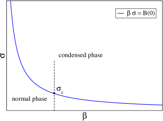
Figure 3: Phase diagram for $d>2$. The dashed vertical line shows the thermodynamic path of the transition driven by $\sigma$ while keeping $\beta$ fixed.

As a consequence of the mode independence, implied by Eq. (37), the $P_{\textrm{MSM}}({\boldsymbol{\varphi}}|\sigma)$ distribution factorizes. Therefore, introducing the notation $\psi_{0}=\frac{1}{V}\varphi_{0}$ for the magnetization density, the $\vec{k}=0$ contribution is given by

$$P_{\textrm{MSM}}({\psi_{0}}|\sigma)=\sqrt{\frac{\beta\widetilde{\kappa}V}{2\pi}}e^{-\frac{\beta\widetilde{\kappa}V}{2}\psi^{2}_{0}},$$ (47)

and inserting the result (46) for $\widetilde{\kappa}$, in the $V\to\infty$ limit the result reported in the main text is obtained

$$\lim_{V\to\infty}P_{\textrm{MSM}}(\psi_{0}|\sigma)=\left\{\begin{array}[]{ll}\delta(\psi_{0}),\;\;$for$\;\;\sigma\leq\sigma_{c},\\ \frac{e^{-\frac{1}{2(\sigma-\sigma_{c})}\psi_{0}^{2}}}{\sqrt{2\pi(\sigma-\sigma_{c})}},\;\;$for$\;\;\sigma>\sigma_{c}.\end{array}\right.$$ (48)

Appendix C The SM - MSM connection

Using the identity $\int_{0}^{\infty}d\sigma^{\prime}\,\delta(\mathit{s}({\boldsymbol{\varphi}})-\sigma^{\prime})=1$, the MSM ensemble (29) can be rewritten as

$$P_{\textrm{MSM}}({\boldsymbol{\varphi}}|\sigma)$$ (49)

$$= \int_{0}^{\infty}d\sigma^{\prime}\,\frac{1}{Z_{\textrm{MSM}}(\sigma)}\,\exp\left\{-\beta[{\cal H}({\boldsymbol{\varphi}})+\frac{\widetilde{\kappa}(\sigma)}{2}\,{\cal S}(\boldsymbol{\varphi})]\right\}$$

$$\times \delta(\mathit{s}({\boldsymbol{\varphi}})-\sigma^{\prime})$$

$$= \int_{0}^{\infty}d\sigma^{\prime}\,\left[\frac{1}{Z_{\textrm{SM}}(\sigma^{\prime})}\,e^{-\beta{\cal H}({\boldsymbol{\varphi}})}\delta(\mathit{s}({\boldsymbol{\varphi}})-\sigma^{\prime})\right]$$

$$\times \,\left[e^{-\beta\frac{\widetilde{\kappa}(\sigma)}{2}V\sigma^{\prime}}\frac{Z_{\textrm{SM}}(\sigma^{\prime})}{Z_{\textrm{MSM}}(\sigma)}\right],$$

which, using the definition (28) of the SM partition function, can be further manipulated as

$$P_{\textrm{MSM}}({\boldsymbol{\varphi}}|\sigma) = \int_{0}^{\infty}d\sigma^{\prime}\,\left[\frac{1}{Z_{\textrm{SM}}(\sigma^{\prime})}\,e^{-\beta{\cal H}({\boldsymbol{\varphi}})}\delta(\mathit{s}({\boldsymbol{\varphi}})-\sigma^{\prime})\right]\,$$ (50)

$$\times \int{\cal D}{\boldsymbol{\varphi}^{\prime}}\,\frac{e^{-\beta\left[{\cal H}({\boldsymbol{\varphi}^{\prime}})+\frac{\widetilde{\kappa}(\sigma)}{2}V\sigma^{\prime}\right]}}{{Z_{\textrm{MSM}}(\sigma)}}\,\delta\left(\mathit{s}(\boldsymbol{\varphi^{\prime}})-\sigma^{\prime}\right)$$

$$= \int_{0}^{\infty}d\sigma^{\prime}\,\left[\frac{1}{Z_{\textrm{SM}}(\sigma^{\prime})}\,e^{-\beta{\cal H}({\boldsymbol{\varphi}})}\delta(\mathit{s}({\boldsymbol{\varphi}})-\sigma^{\prime})\right]\,$$

$$\times \int{\cal D}{\boldsymbol{\varphi}^{\prime}}\,\frac{e^{-\beta\left[{\cal H}({\boldsymbol{\varphi}^{\prime}})+\frac{\widetilde{\kappa}(\sigma)}{2}{\cal S}(\boldsymbol{\varphi^{\prime}})\right]}}{{Z_{\textrm{MSM}}(\sigma)}}\,$$

$$\times \delta\left(\mathit{s}(\boldsymbol{\varphi^{\prime}})-\sigma^{\prime}\right).$$

Recognizing that in the square bracket there appears $P_{\textrm{SM}}({\boldsymbol{\varphi}}|\sigma^{\prime})$, while the last integral

$$K_{\textrm{MSM}}(\sigma^{\prime}|\sigma)=\int{\cal D}{\boldsymbol{\varphi}^{\prime}}\,\frac{e^{-\beta\left[{\cal H}({\boldsymbol{\varphi}^{\prime}})+\frac{\widetilde{\kappa}(\sigma)}{2}{\cal S}(\boldsymbol{\varphi^{\prime}})\right]}}{{Z_{\textrm{MSM}}(\sigma)}}\,\delta\left(\mathit{s}(\boldsymbol{\varphi^{\prime}})-\sigma^{\prime}\right)$$ (51)

is the probability that $\mathit{s}(\boldsymbol{\varphi})$ takes the value $\sigma^{\prime}$ in the MSM parametrized by $\sigma$, the probabilities of $\boldsymbol{\varphi}$ in the two models are related by

$$P_{\textrm{MSM}}({\boldsymbol{\varphi}}|\sigma)=\int_{0}^{\infty}d\sigma^{\prime}\,P_{\textrm{SM}}({\boldsymbol{\varphi}}|\sigma^{\prime})\,K_{\textrm{MSM}}(\sigma^{\prime}|\sigma).$$ (52)

Eliminating the $\varphi_{\vec{k}\neq 0}$ components from the above equation by integration, a similar relation is obtained between the $\psi_{0}$ marginal distributions

$$P_{\textrm{MSM}}({\psi_{0}}|\sigma)=\int_{0}^{\infty}d\sigma^{\prime}\,P_{\textrm{SM}}({\psi_{0}}|\sigma^{\prime})\,K_{\textrm{MSM}}(\sigma^{\prime}|\sigma).$$ (53)

The kernel $K_{\textrm{MSM}}(\sigma^{\prime}|\sigma)$ has been computed by Kac and Thompson KT obtaining

$$K_{\textrm{MSM}}(\sigma^{\prime}|\sigma)=\delta(\sigma^{\prime}-\sigma),\quad\text{for}\quad\sigma<\sigma_{c},$$ (54)

and for $\sigma>\sigma_{c}$

$$K_{\textrm{MSM}}(\sigma^{\prime}|\sigma)=\begin{cases}0,\quad$for$\quad\sigma^{\prime}<\sigma_{c},\\ \phantom{x}&\phantom{x}\\ \frac{\exp\left\{-\frac{\sigma^{\prime}-\sigma_{c}}{2(\sigma-\sigma_{c})}\right\}}{\sqrt{2\pi(\sigma^{\prime}-\sigma_{c})(\sigma-\sigma_{c})}},\quad\text{for}\quad\sigma^{\prime}>\sigma_{c}.\end{cases}$$ (55)

Therefore, using the above result together with Eq. (12), one can check that for $\sigma<\sigma_{c}$ Eq. (53) is solved by

$$P_{\textrm{SM}}({\psi_{0}}|\sigma)=\delta(\psi_{0}),$$ (56)

while for $\sigma>\sigma_{c}$ one gets

$$\frac{\exp\left\{-\frac{\psi_{0}^{2}}{2(\sigma-\sigma_{c})}\right\}}{\sqrt{2\pi(\sigma-\sigma_{c})}}=\int_{\sigma_{c}}^{\infty}d\sigma^{\prime}\,P_{\textrm{SM}}({\psi_{0}}|\sigma^{\prime})\,\frac{\exp\left\{-\frac{\sigma^{\prime}-\sigma_{c}}{2(\sigma-\sigma_{c})}\right\}}{\sqrt{\sigma^{\prime}-\sigma_{c}}},$$ (57)

from which follows

$$P_{\textrm{SM}}({\psi_{0}}|\sigma) = \sqrt{\sigma-\sigma_{c}}\;\delta[\sigma-\sigma_{c}-\psi_{0}^{2}]$$

$$= \frac{1}{2}[\delta(\psi_{0}+\sqrt{\sigma-\sigma_{c}})+\delta(\psi_{0}-\sqrt{\sigma-\sigma_{c}})].$$

Appendix D The CE - GCE connection in the ideal Bose gas

The Fock space representation of the Hamiltonian $\widehat{{\cal H}}=\sum_{\vec{k}}\epsilon_{k}\widehat{a}^{\dagger}_{\vec{k}}\widehat{a}_{\vec{k}}$ and number operator $\widehat{{\cal N}}=\sum_{\vec{k}}\widehat{a}^{\dagger}_{\vec{k}}\widehat{a}_{\vec{k}}$ is given by

$$\widehat{{\cal H}}=\sum_{\boldsymbol{n}}E(\boldsymbol{n})|\boldsymbol{n}\rangle\langle\boldsymbol{n}|,$$ (59)

$$\widehat{{\cal N}}=\sum_{\boldsymbol{n}}N(\boldsymbol{n})|\boldsymbol{n}\rangle\langle\boldsymbol{n}|,$$ (60)

where $\boldsymbol{n}$ stands for a collection $[n_{\vec{k}}]$ of occupation numbers, $|\boldsymbol{n}\rangle$ are the product states $\prod_{\vec{k}}|n_{\vec{k}}\rangle$ and the eigenvalues are given by

$$E(\boldsymbol{n})=\sum_{\vec{k}}\epsilon_{k}n_{\vec{k}},$$ (61)

$${\cal N}(\boldsymbol{n})=\sum_{\vec{k}}n_{\vec{k}}.$$ (62)

It is first convenient to lay out the general relation between the Fock-space and the Glauber-Sudarshan representations Glauber ; Sudarshan of the density matrix

$$D=\sum_{\boldsymbol{n}}P(\boldsymbol{n})|\boldsymbol{n}\rangle\langle\boldsymbol{n}|=\int d^{2}\boldsymbol{\alpha}\,P(\boldsymbol{\alpha})|\boldsymbol{\alpha}\rangle\langle\boldsymbol{\alpha}|,$$ (63)

where $|\boldsymbol{\alpha}\rangle=\prod_{\vec{k}}|\alpha_{\vec{k}}\rangle$. The $\vec{k}$-mode coherent state $|\alpha_{\vec{k}}\rangle$ is an eigenvector of the annihilation operator $\widehat{a}_{\vec{k}}|\alpha_{\vec{k}}\rangle=\alpha_{\vec{k}}|\alpha_{\vec{k}}\rangle$ with complex eigenvalue $\alpha_{\vec{k}}$. The weight functions are related by

$$P(\boldsymbol{n})=\int d^{2}\boldsymbol{\alpha}\,R(\boldsymbol{n}|\boldsymbol{\alpha})P(\boldsymbol{\alpha}),$$ (64)

with the kernel

$$R(\boldsymbol{n}|\boldsymbol{\alpha})=|\langle\boldsymbol{n}|\boldsymbol{\alpha}\rangle|^{2}=\prod_{\vec{k}}e^{-|\alpha_{\vec{k}}|^{2}}\frac{|\alpha_{\vec{k}}|^{2n_{\vec{k}}}}{(n_{\vec{k}})!}.$$ (65)

The canonical and the grand canonical ensembles are obtained by controlling the density of particles $\rho$ either strictly or on average. Then, the corresponding density matrices are given by

$$D_{\textrm{CE}}(\rho)=\sum_{\boldsymbol{n}}P_{\textrm{CE}}(\boldsymbol{n}|\rho)|\boldsymbol{n}\rangle\langle\boldsymbol{n}|,$$ (66)

$$D_{\textrm{GCE}}(\rho)=\sum_{\boldsymbol{n}}P_{\textrm{GCE}}(\boldsymbol{n}|\rho)|\boldsymbol{n}\rangle\langle\boldsymbol{n}|,$$ (67)

where the weight functions read

$$P_{\textrm{CE}}(\boldsymbol{n}|\rho)=\frac{1}{Z_{\textrm{CE}}}e^{-\beta E(\boldsymbol{n})}\,\delta_{{\cal N},V\rho},$$ (68)

$$P_{\textrm{GCE}}(\boldsymbol{n}|\rho)=\frac{1}{Z_{\textrm{GCE}}}e^{-\beta[E(\boldsymbol{n})-\mu{\cal N}(\boldsymbol{n})]}.$$ (69)

In the latter one the chemical potential $\mu$ is fixed by the condition

$$\frac{1}{V}\langle{\cal N}\rangle_{\textrm{GCE}}=\rho.$$ (70)

By going through the same algebra as in the preceding section it is straightforward to verify that these weights obey the relation analogous to Eq. (52)

$$P_{\textrm{GCE}}(\boldsymbol{n}|\rho)=\int_{0}^{\infty}d\rho^{\prime}\,P_{\textrm{CE}}(\boldsymbol{n}|\rho^{\prime})K_{\textrm{GCE}}(\rho^{\prime}|\rho),$$ (71)

where $K_{\textrm{GCE}}(\rho^{\prime}|\rho)$ is the probability that the particle density takes the value $\rho^{\prime}$ in the GCE controlled by the average value $\rho$,

$$K_{\textrm{GCE}}(\rho^{\prime}|\rho)=\sum_{\boldsymbol{n}}P_{\textrm{GCE}}(\boldsymbol{n}|\rho)\,\delta_{{\cal N}(\boldsymbol{n}),V\rho^{\prime}}.$$ (72)

This is given by the Kac function Ziff , which for $\rho<\rho_{c}$ reads

$$K_{\textrm{GCE}}(\rho^{\prime}|\rho)=\delta(\rho^{\prime}-\rho),\quad\text{for}\quad\rho<\rho_{c},$$ (73)

while for $\rho>\rho_{c}$ is given by

$$K_{\textrm{GCE}}(\rho^{\prime}|\rho)=\begin{cases}0,\quad$for$\quad\rho^{\prime}<\rho_{c},\\ \phantom{x}&\phantom{x}\\ \frac{\exp\left\{-\frac{\rho^{\prime}-\rho_{c}}{\rho-\rho_{c}}\right\}}{\rho-\rho_{c}},\quad\text{for}\quad\rho^{\prime}>\rho_{c}.\end{cases}$$ (74)

Next, inserting Eq. (64) into Eq. (71) and taking into account that the kernel $R(\boldsymbol{n}|\boldsymbol{\alpha})$ is positive definite, the analogous relation is found to hold between the P-representation weight functions

$$P_{\textrm{GCE}}(\boldsymbol{\alpha}|\rho)=\int_{0}^{\infty}d\rho^{\prime}\,P_{\textrm{CE}}(\boldsymbol{\alpha}|\rho^{\prime})K_{\textrm{GCE}}(\rho^{\prime}|\rho).$$ (75)

Integrating this over all $\alpha_{\vec{k}\neq 0}$, eventually one finds

$$P_{\textrm{GCE}}(\alpha_{0}|\rho)=\int_{0}^{\infty}d\rho^{\prime}\,P_{\textrm{CE}}(\alpha_{0}|\rho^{\prime})K_{\textrm{GCE}}(\rho^{\prime}|\rho),$$ (76)

where the left hand side term is given by Glauber

$$P_{\textrm{GCE}}(\alpha_{0}|\rho)=\frac{1}{\pi\langle n_{0}\rangle}e^{-\frac{|\alpha_{0}|^{2}}{\langle n_{0}\rangle}},$$ (77)

with

$$\langle n_{0}\rangle=[e^{-\beta\widetilde{\mu}(\rho)}-1]^{-1}=\begin{cases}O(1),\quad$for$\quad\rho<\rho_{c},\\ \phantom{x}&\phantom{x}\\ V(\rho-\rho_{c}),\quad\text{for}\quad\rho>\rho_{c},\end{cases}$$ (78)

having denoted by $\widetilde{\mu}(\rho)$ the solution of Eq. (70) with respect to $\mu$. Therefore, defining $\eta_{0}=\alpha_{0}/\sqrt{V}$ and inserting Eqs. (73,74,76,77) into Eq. (75), it is easy to verify that in the large $V$ limit for $\rho<\rho_{c}$

$$P_{\textrm{GCE}}(|\eta_{0}||\rho)=P_{\textrm{CE}}(|\eta_{0}||\rho)=\delta(|\eta_{0}|),$$ (79)

while for $\rho>\rho_{c}$

$$P_{\textrm{GCE}}(|\eta_{0}||\rho)=\frac{1}{\pi(\rho-\rho_{c})}e^{-\frac{|\eta_{0}|^{2}}{\rho-\rho_{c}}},$$ (80)

and

$$P_{\textrm{CE}}(|\eta_{0}||\rho)=\frac{1}{\pi}\delta(|\eta_{0}|^{2}-(\rho-\rho_{c})).$$ (81)

References

(1)
K. Huang, Statistical Mechanics, John Wiley and Sons, New York 1967.
(2)
R. K. Pathria and P. D. Beale, Statistical Mechanics 3d Edition, Elsevier, Burlington 2011.
(3)
A. Puglisi, A. Sarracino, A. Vulpiani,
Phys. Rep. 709-710, 1 (2017).
(4)
For a review see A. Campa, T. Dauxois, S. Ruffo, Phys. Rep. 480, 57 (2009).
(5)
R. M. Ziff, G. E. Uhlenbeck and M. Kac, Phys. Rep. 32, 169 (1977).
(6)
M. Holthaus and K. Kirsten, Ann. of Phys. 270, 198 (1998).
(7)
I. Fujiwara, D. ter Haar and H. Wergeland, J. Stat. Phys. 2, 329 (1970).
(8)
L. Pitaevskii and S. Stringari, Bose-Einstein Condensation, Oxford University Press - New York (2003).
(9)
Vitaly V. Kocharovsky, Vladimir V. Kocharovsky, M. Holthaus, C. H. Raymond Ooi, A. A. Svidzinsky,
W. Ketterle, M. O. Scully,
Adv. in Atomic, Molecular and Opt. Phys., 53, 291 (2006).
(10)
V. I. Yukalov, Laser Phys. Lett. 4, 632 (2007); Annals of Physics 323, 461 (2008);
Phys. Part. Nuclei 42, 460 (2011).
(11)
J. Klaers, J. Schmitt, F. Vewinger and M.Weitz, Nature 468, 545 (2010)
(12)
J. Schmitt, T. Damm, D. Dung, F. Vewinger, J. Klaers and M. Weitz, Phys. Rev. Lett. 112, 030401 (2014).
(13)
M. Kac and C. J. Thompson, J. Math. Phys. 18, 1650 (1977).
(14)
M. Kac, in The Physicist’s Conception of Nature, edited by
J. Mehra (Reidel, Dordrecht, 1973), p. 521.
(15)
J. T. Cannon, Commun. Math. Phys. 29, 89 (1973).
(16)
S. K. Ma, Modern Theory of Critical Phenomena, W A Benjamin (1976);
D. J. Amit and V. Martín-Mayor, Field Theory, the Renormalization Group, and Critical Phenomena, World Scientific Singapore (2005).
(17)
T. H. Berlin and M. Kac, Phys. Rev. 86, 821 (1952).
(18)
H. W. Lewis and G. H. Wannier, Phys. Rev. 88, 682 (1952) and
Phys. Rev. 90, 1131E (1953).
(19)
The relation between BEC and fluctuations in the GCE is discussed
in detail in M. Zannetti, EPL 111, 20004 (2015).
(20)
C. Castellano, F. Corberi and M. Zannetti, Phys. Rev. E 56, 4973 (1997);
N. Fusco and M. Zannetti, Phys. Rev. E 66, 066113 (2002).
(21)
F. Corberi, G. Gonnella, A. Piscitelli and M. Zannetti, J. Phys. A: Math. Theor. 46, 042001 (2013);
M. Zannetti, F. Corberi and G. Gonnella, Phys. Rev. E 90, 012143 (2014); M.Zannetti,
F. Corberi, G. Gonnella and A. Piscitelli, Commun. Theor. Phys. 62, 555 (2014).
(22)
N. Merhav and Y. Kafri, J. Stat. Mech. P02011 (2010).
(23)
M. Filiasi, G.Livan, M. Marsili. M. Peressi, E. Vesselli and E. Zarinelli, J. Stat. Mech. P09030 (2014);
M. Filiasi, E. Zarinelli, E. Vesselli and M. Marsili, arXiv:1309.7795v1;
L. Ferretti, M. Mamino and G. Bianconi, Phys. Rev. E 89, 042810 (2014).
(24)
R. J. Galuber, Phys. Rev. 131, 2766 (1963).
(25)
E. C. G. Sudarshan, Phys. Rev. Lett. 10, 277 (1963).
(26)
J. Klaers, M. Weitz, Bose-Einstein condensation of photons and grand-canonical condensate fluctuations
in Universal Themes of Bose-Einstein Condensation, Cambridge University Press (2017),
edited by Nick P. Proukakis, David W. Snoke, Peter B. Littlewood, pag. 391