Double parton interaction: the values of $\sigma_{\rm eff}$

Abstract

In this letter we show that the two parton showers mechanism for $J/\Psi$ production, that has been discussed in Ref.LESI , leads to small values of $\sigma_{\rm eff}$ for the production of a pair of $J/\Psi$. We develop a simple two channel approach to estimate the values of $\sigma_{\rm eff}$, which produces values that are in accord with the experimental data.

.1 Introduction

The double parton interaction has been under close scrutiny over the past three decades both by theoreticians (see Ref.DIGA and references therein) and by the experimentalistsAFSC ; UA2 ; CDF ; CDF2 ; D0 ; LHCB ; ATLAS ; CMS ; ATLAS2 ; D01 ; LHCB1 ; ATLAS3 ; CMS1 ; ATLAS4 ; D03 ; ATLAS5 ; LHCB3 ; D04 ; CMS2 ; ATLAS7 ; LHCB4 ; D05 ; D06 ; ATLAS6 ; CMS3 . The fairly large cross sections for the double parton interaction at high energy support the assumption, that a dense system of partons is produced in the proton-proton collisions at high energy. Such dense systems of partons appears naturally in the CGC/saturation approach to high energy QCDKOLEB , which permits us to consider hadron-hadron, hadron-nucleus and nucleus-nucleus interactions from a unique point of view. As a quantitive measure of the strong double parton interaction, the value of $\sigma_{\rm eff}$ is used, this was introduced by considering the double inclusive cross sections of two pairs of back-to-back jets with momenta $p_{T,1}$ and $p_{T,2}$, measured with rapidities of two pairs ($y_{1}$ and $y_{2}$), which are close to each other ($y_{1}\approx y_{2}$, see Fig. 1). These pairs can only be produced from two different parton showers. The data were parameterized in the form

$$\frac{d\sigma}{dy_{1}d^{2}p_{T,1}dy_{2}d^{2}p_{T,2}}\,\,=\,\,\frac{m}{2\sigma_{eff}}\,\frac{d\sigma}{dy_{1}d^{2}p_{T,1}}\frac{d\sigma}{dy_{2}d^{2}p_{T,2}}$$ (1)

where $m=2$ for different pairs of jets and $m=1$ for identical pairs. The values of $\sigma_{\rm eff}$ are shown in Fig. 2 for different final states.

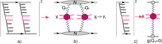
Figure 1: Two parton showers contribution to two pairs of back-to-back gluon jet production in hadron-hadron collisions (Fig. 1-a). Helical lines denote the gluons. The red helical lines depict the jets. The wavy lines describe the BFKL Pomeron. Fig. 1-b shows the Mueller diagramMUDI for the double inclusive cross section, while Fig. 1-c is the Mueller diagram for the inclusive cross section.

One can see from this figure, that in spite of large errors, pairs $J/\Psi+J/\Psi$ and $J/\Psi+\Upsilon$ have a small value of $\sigma_{\rm eff}$ of about 5 mb, while other final states lead to $\sigma_{\rm eff}\,of\approx$ 15 mb.

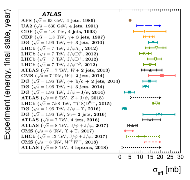
Figure 2: Summary of measurements and limits on the effective cross section, determined in different experimentsAFSC ; UA2 ; CDF ; CDF2 ; D0 ; LHCB ; ATLAS ; CMS ; ATLAS2 ; D01 ; LHCB1 ; ATLAS3 ; CMS1 ; ATLAS4 ; D03 ; ATLAS5 ; LHCB3 ; D04 ; CMS2 ; ATLAS7 ; LHCB4 ; D05 ; D06 ; ATLAS6 ; CMS3 . The measurements that were made by different experiments are denoted by different symbols and colours. The figure is taken from Ref.ATLAS7 .

In this letter we wish to show that the two parton shower mechanism for $J/\Psi$ production, that has been discussed in Ref.LESI , leads to small values of $\sigma_{\rm eff}$, and also to develop a simple two channel approach to estimate the values of $\sigma_{\rm eff}$.

.2 $\sigma_{\rm eff}$ in the BFKL Pomeron calculus

The double inclusive cross section for two pairs of the jets shown in Fig. 1 can be written in the form (see Fig. 1-b)

$$\frac{d\sigma}{dy_{1}d^{2}p_{T,1}dy_{2}d^{2}p_{T,2}}\,\,=\,\,\int\frac{d^{2}\,Q_{T}}{4\pi^{2}}\,\frac{N^{2}\left(Q_{T}\right)}{g^{4}\left(Q_{T}=0\right)}\frac{d\sigma}{dy_{1}d^{2}p_{T,1}}\left(Q_{T}\right)\frac{d\sigma}{dy_{2}d^{2}p_{T,2}}\left(Q_{T}\right)$$ (2)

In Eq. (2) $\frac{d\sigma}{dy_{1}d^{2}p_{T,1}}\left(Q_{T}\right)$ describes the production of two back-to-back jets from the BFKL PomeronBFKL and can be written in the form:

$$\frac{d\sigma}{dy_{1}d^{2}p_{T,1}}\left(Q_{T}\right)\,\,=\,\,G^{\rm BFKL}_{I\!\!P}\left(Y-y_{1},k_{T},Q_{T}\right)\bigotimes\sigma_{\rm hard}\bigotimes G^{\rm BFKL}_{I\!\!P}\left(y_{2},\boldsymbol{p}_{1,T}+\boldsymbol{p}_{2,T}-\boldsymbol{k}_{T};Q_{T}\right)$$ (3)

where $\bigotimes$ stands for all necessary integrations and $Q_{T}$ denotes the transverse momentum. The amplitude of the BFKL Pomeron $G^{\rm BFKL}_{I\!\!P}\left(Y-y_{1},k_{T},Q_{T}\right)$ can be simplified if we take into account that the $\boldsymbol{Q}_{T}$ dependence of the BFKL Pomeron is determined by the size of the largest of the interacting dipoles . Indeed, in this case $Q_{T}\approx 1/R_{h}\,\,\ll\,\,k_{T}(p_{T})$ and the $Q_{T}$ dependence can be described by $g\left(Q_{T}\right)$ in Eq. (5), which has a non-perturbative origin and, in practice, has to be taken from the experiment.

$$G_{I\!\!P}^{\rm BFKL}\left(Y-y_{1},k_{T},Q_{T}\right)\,\,\approx\,\,G_{I\!\!P}^{\rm BFKL}\left(Y-y_{1},k_{T},Q_{T}=0\right)\,g\left(Q_{T}\right)$$ (5)

Eq. (5) has a simple interpretation in the framework of the BFKL Pomeron calculus (see Ref.KOLEB for a review): $G_{I\!\!P}^{\rm BFKL}$ describes the BFKL Pomeron Green’s function, while $g\left(Q_{T}\right)$ denotes the vertex of interaction of the Pomeron with the hadron.

For the exchange of two BFKL Pomerons in Eq. (2) we assume that dependence on $Q_{T}\sim 1/R_{h}$ is described by the function $N\left(Q_{T}\right)$, which can be treated as a phenomenological amplitude of the interaction of two BFKL Pomerons with the hadron. It is worth mentioning that the first contribution to $N\left(Q_{T}\right)=g^{2}\left(Q_{T}\right)$, which corresponds to the contribution of the eikonal rescattering on the hadron to this amplitude (see Fig. 3-a1). Therefore, we have

$$\frac{d\sigma}{dy_{1}d^{2}p_{T,1}dy_{2}d^{2}p_{T,2}} = \int\frac{d^{2}\,Q_{T}}{4\pi^{2}}\,N^{2}\left(Q_{T}\right)\times\,\Bigg{\{}G^{\rm BFKL}_{I\!\!P}\left(Y-y_{1},k_{T},0\right)\bigotimes\sigma_{\rm hard}\bigotimes\,G^{\rm BFKL}_{I\!\!P}\left(y_{2},\boldsymbol{p}_{1,T}+\boldsymbol{p}_{2,T}-\boldsymbol{k}_{T};0\right)$$ (6)

$$\times \,G^{\rm BFKL}_{I\!\!P}\left(Y-y_{1},k_{T},0\right)\bigotimes\sigma_{\rm hard}\bigotimes\,G^{\rm BFKL}_{I\!\!P}\left(y_{2},\boldsymbol{p}_{1,T}+\boldsymbol{p}_{2,T}-\boldsymbol{k}_{T};\boldsymbol{Q},0\right)\Bigg{\}}$$

Finally, with these assumptions we can re-write Eq. (2) as follows:

$$\frac{d\sigma}{dy_{1}d^{2}p_{T,1}dy_{2}d^{2}p_{T,2}}\,\,=\,\,\int\frac{d^{2}\,Q_{T}}{4\pi^{2}}\,\frac{N^{2}\left(Q_{T}\right)}{g^{4}\left(Q_{T}=0\right)}\frac{d\sigma}{dy_{1}d^{2}p_{T,1}}\left(Q_{T}=0\right)\frac{d\sigma}{dy_{2}d^{2}p_{T,2}}\left(Q_{T}=0\right)$$ (7)

Eq. (3) takes the form:

$$\frac{d\sigma}{dy_{1}d^{2}p_{T,1}}\left(Q_{T}=0\right)\,\,=\,g^{2}\left(Q_{T}=0\right)\,\Bigg{\{}G^{\rm BFKL}_{I\!\!P}\left(Y-y_{1},k_{T},0\right)\bigotimes\sigma_{\rm hard}\bigotimes G^{\rm BFKL}_{I\!\!P}\left(y_{2},\boldsymbol{p}_{1,T}+\boldsymbol{p}_{2,T}-\boldsymbol{k}_{T};0\right)\Bigg{\}}$$ (8)

which leads to

$$\frac{1}{\sigma_{\rm eff}}\,=\,\int\frac{d^{2}\,Q_{T}}{4\pi^{2}}\,\frac{N^{2}\left(Q_{T}\right)}{g^{4}\left(Q_{T}=0\right)}$$ (9)

Note, that the factors, that stem from short distances and are denoted by $\{\dots\}$ in Eq. (6) and Eq. (8), cancel in Eq. (9).

The principal feature of Eq. (9) is that the value of $\sigma_{\rm eff}$ does not depend on the nature of the hard process. This could be the di-jet production, the inclusive production of $J/\Psi$ or any of the hard processes shown in Fig.2, however Eq. (9) should be the same. As one can see from Fig.2, that experimentally for vast number of different hard processes, we have more or less the same values of $\sigma_{\rm eff}$ . However, for $J/\Psi$ production the value of $\sigma_{\rm eff}$ turns out to be smaller than for other processes, in spite of the fact that at first sight we can use the same Eq. (9) for its value. Actually, $\sigma_{\rm eff}$ characterizes typical long distances that contribute to the hard processes. In the case of single inclusive production we are able to include these long distances in the experimental parton densities. However, for the double inclusive production we have to introduce more information regarding these contributions. In our approach we introduce the functions $N\left(Q_{T}\right)$.

$N\left(Q_{T}\right)$ denotes the scattering amplitude of the BFKL Pomeron with the hadron integrated over all produced mass, which has a non-perturbative origin, and should be taken from non-perturbative QCD, or from high energy phenomenology, bearing in mind the current embryonic stage of the non-perturbative approach. Eq. (2) is discussed in more detail in Ref.LERE . The amplitude $N(Q_{T})$ has a complex structure and can be viewed as the sum of the elastic contribution and the inelastic one, and should be summed over the entire range of the produced mass (see Fig. 3-a).

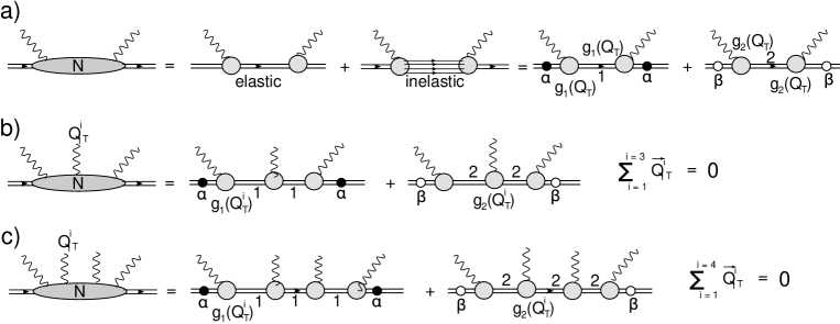
Figure 3: The structure of the amplitude $N$ in the two channel model.

In the two channel approximation we replace the rich structure of the produced states, by a single state with the wave function $\psi_{D}$. The observed physical hadronic and diffractive states are written in the form

$$\psi_{h}\,=\,\alpha\,\Psi_{1}+\beta\,\Psi_{2}\,;\,\,\,\,\,\,\,\,\,\,\psi_{D}\,=\,-\beta\,\Psi_{1}+\alpha\,\Psi_{2};~{}~{}~{}~{}~{}~{}~{}~{}~{}\mbox{where}~{}~{}~{}~{}~{}~{}~{}\alpha^{2}+\beta^{2}\,=\,1;$$ (10)

Functions $\psi_{1}$ and $\psi_{2}$ form a complete set of orthogonal functions $\{\psi_{i}\}$ which diagonalize the interaction matrix ${\bf T}$

$$A^{i^{\prime}k^{\prime}}_{i,k}=<\psi_{i}\,\psi_{k}|\mathbf{T}|\psi_{i^{\prime}}\,\psi_{k^{\prime}}>=A_{i,k}\,\delta_{i,i^{\prime}}\,\delta_{k,k^{\prime}}.$$ (11)

Bearing Eq. (11) in mind, we can write the following expression for the amplitude $N$ (see Fig. 3-a):

$$N\left(Q_{T}\right)\,\,=\,\,\alpha^{2}g^{2}_{1}\left(Q_{T}\right)\,\,+\,\,\beta^{2}g^{2}_{2}\left(Q_{T}\right)$$ (12)

In Eq. (12) the first term corresponds to the contribution of the state $\Psi_{1}$ and the second of the state $\Psi_{2}$, to the amplitude of the interaction of two Pomerons with the nucleon.

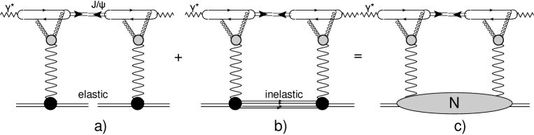
Figure 4: Diffractive production of the $J/\Psi$ meson in deep inelastic scattering at low $x$. Wavy lines denote the BFKL Pomerons.

$g_{i}(Q_{T})$ are phenomenological functions, while $\alpha$ is a constant whose value we determine by fitting to the experimental data. Fortunately, we can determine the values of $g_{i}(Q_{T})$ and $\alpha$ by considering the diffractive production of $J/\Psi$ in DISH1DD ; H1DD1 ; ZEUS1 . These data indicate that the diffractive production of $J/\Psi$ has different slopes in $Q_{T}$, for elastic (see Fig. 4-a) and for inelastic (see Fig. 4-b) production. For the reaction $\gamma^{*}+p\to J/\Psi+p$, $d\sigma_{el.\,diff}/dQ^{2}_{T}\propto\exp\left(-B_{el}Q^{2}_{T}\right)$ with $B_{el}\approx 5\,GeV^{-2}$, while for $\gamma^{*}+p\to J/\Psi+X$ the slope turns out to be much smaller $d\sigma_{inel.\,diff}/dQ^{2}_{T}\propto\exp\left(-B_{in}Q^{2}_{T}\right)$ with $B_{in}\approx 1.69\,GeV^{-2}$. The second conclusion from the data is that the cross sections of elastic and inelastic $J/\Psi$ diffractive production are the same. We can implement the described features of the diffractive production of $J/\Psi$ by introducing $g_{1}\left(Q_{T}\right)=g_{1}e^{-\frac{1}{2}B_{1}\,Q^{2}_{T}}$ and $g_{2}\left(Q_{T}\right)=g_{1}e^{-\frac{1}{2}B_{2}\,Q^{2}_{T}}$ and imposing the following restrictions on the parameters

$$B_{1}=B_{el};~{}~{}B_{2}=B_{in};~{}~{}~{}~{}\alpha^{2}\frac{g^{2}_{1}}{B_{1}}\,=\,\beta^{2}\frac{g_{2}^{2}}{B_{2}}$$ (13)

These equations for $B_{i}$ follows from the fact that function $\Psi_{1}$ gives the main contribution to the for elastic diffractive production, while $\Psi_{2}$ is introduced to describe the inelastic diffraction.

Plugging Eq. (3) into Eq. (2) we have

$$\frac{1}{\sigma_{\rm eff}}\,=\,\int\frac{d^{2}\,Q_{T}}{4\pi^{2}}\,\frac{\left(\alpha^{2}g^{2}_{1}\left(Q_{T}\right)+\beta\,g^{2}_{2}\left(Q_{T}\right)\right)^{2}}{\left(\alpha^{2}g_{1}\left(0\right)+\beta^{2}g_{2}\left(0\right)\right)^{4}}$$ (14)

In Fig. 5 we plot the value of $\sigma_{\rm eff}$ for a pair of back-to-back jets.

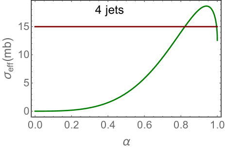
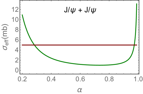
Fig. 5-a	Fig. 5-b

Figure 5: $\sigma_{\rm eff}$ for a pair of back-to-back jets (see Fig. 5-a and Eq. (2)), and for pair of $J/\Psi$ (Fig. 5-b). The red lines show $\sigma_{\rm eff}$ = 15 mb in Fig. 5-a and $\sigma_{\rm eff}$ = 5 mb in Fig. 5-b.

We reach the average experimental value of $\sigma_{\rm eff}=15\,mb$ at $\alpha=0.8$. It should be noted that the information that we obtain from the diffractive production of $J/\Psi$, is enough to claim that $\sigma_{\rm eff}\leq 20\,mb$ in a two channel model.

.3 $\sigma_{\rm eff}$ for the production $J/\Psi$ and $\Upsilon$ pairs

.3.1 Two parton showers mechanism for $J/\Psi$ production

In Ref.LESI it is shown that the two parton shower mechanism of $J/\Psi$ production, which is illustrated in Fig. 6, gives the description of total and differential cross sections. In this paper we would like to show that this mechanism leads to a value of $\sigma_{\rm eff}$ which is much smaller than the one of the previous section. The formula for the single inclusive cross section of $J/\Psi$ prodiuction with transverse momentum $q_{T}$ is given in Ref.LESI and has the following form

$$\frac{d\sigma\left(Y,\,Q^{2}\right)}{dy\,d^{2}q_{T}}\,\, = \,\,\frac{4\,C_{F}^{3}\,\bar{\alpha}_{S}^{3}}{(2\pi)^{4}}\,\int\frac{d^{2}Q_{T}}{(2\pi)^{2}}\,g\left(0\right)\,N\left(Q_{T}\right)\,\int d^{2}k_{T}d^{2}p_{T}\,\,G_{I\!\!P}^{\rm BFKL}\left(Y-y,\,p_{T},\,0\right)\,$$

$$\times I^{2}\left(\boldsymbol{k}_{T},\,\boldsymbol{q}_{T}\right)\,G_{{I\!\!P}}^{{\rm BFKL}}\left(y;\,\boldsymbol{k}_{T}+\frac{1}{2}\boldsymbol{q}_{T},\,0\right)\,G_{{I\!\!P}}^{{\rm BFKL}}\left(y,-\boldsymbol{k}_{T}+\frac{1}{2}\boldsymbol{q}_{T},\,0\right)$$

$$= \int d^{2}Q_{T}\,g\left(0\right)\,N\left(Q_{T}\right)\,\Bigg{\{}\int d^{2}k_{T}d^{2}p_{T}\,\,G_{I\!\!P}^{\rm BFKL}\left(Y-y,\,p_{T},\,0\right)\,$$

$$\times V\left(k_{T},q_{T}\right)\,G_{{I\!\!P}}^{{\rm BFKL}}\left(y;\,\boldsymbol{k}_{T}+\frac{1}{2}\boldsymbol{q}_{T},\,0\right)\,G_{{I\!\!P}}^{{\rm BFKL}}\left(y,-\boldsymbol{k}_{T}+\frac{1}{2}\boldsymbol{q}_{T},\,0\right)\Bigg{\}}$$

$$\propto \,\,\int d^{2}Q_{T}\,g\left(0\right)\,N\left(Q_{T}\right)$$ (15c)

Eq. (15) is rewritten in Eq. (15) in the form, which correspond the Mueller diagram of Fig. 6, and introduces the triple Pomeron vertex with emitted $J/\Psi$ ($V$ in Fig. 6) in the explicit form. Function $I\left(\boldsymbol{k}_{T},\,\boldsymbol{q}_{T}\right)$ is given in Ref.LESI . In this equation the expression in $\{\dots\}$ does not depend on $Q_{T}$ and stems from the short distances. In the same way as these short distance contributions cancel in the expression for $\sigma_{\rm eff}$ of Eq. (9), they will not contribute to the value of $\sigma_{\rm eff}$ for double $J/\Psi$ or $\Upsilon$ productions.

Therefore, one can see from Fig. 6 the single inclusive production of $J/\Psi$ is proportional to

$$\frac{d\sigma}{dy_{1}} \,\propto \,g(Q_{T}=0)\int\frac{d^{2}\,Q_{T}}{4\pi^{2}}N\left(Q_{T}\right)\,=\,\left(\alpha^{2}g_{1}(Q_{T}=0)+\beta^{2}g_{2}(Q_{T}=0)\right)\int\frac{d^{2}\,Q_{T}}{4\pi^{2}}\left(\alpha^{2}\,g^{2}_{1}(Q_{T}=0)\,+\,\beta^{2}g^{2}_{2}(Q_{T})\right)\,$$ (16)

$$= \,\frac{1}{4\pi}\left(\alpha^{2}g_{1}+\beta^{2}g_{2}\right)\left(\alpha^{2}\frac{g^{2}_{1}}{B_{1}}\,+\,\beta^{2}\frac{g^{2}_{2}}{B_{2}}\right)\,\,=\,\,\frac{1}{4\pi}2\left(\alpha^{2}g_{1}+\beta^{2}g_{2}\right)\left(\alpha^{2}\frac{g^{2}_{1}}{B_{1}}\right)$$

Eq. (16) is the generalization to two channel model of Eq. (15), which is written for the eikonal approach in which $N\left(Q_{T}\right)=g^{2}\left(Q_{T}\right)$.

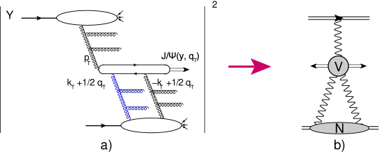
Figure 6: The two parton shower mechanism for $J/\Psi$ production (see Fig. 6-a). Fig. 6-b shows the Mueller diagramMUDI for the inclusive $J/\Psi$ production. The wavy lines describe the BFKL Pomerons. The vertex V is defined in Eq. (15).

.3.2 Double inclusive productions $J/\Psi$ and $\Upsilon$

The Mueller diagrams for the double inclusive cross section of $J/\Psi$ pair production are shown in Fig. 7. From this figure we see that the double inclusive cross section can be estimated using the amplitudes of the interaction with three and four Pomerons, which are shown in Fig. 3-b and Fig. 3-c. Using these amplitudes, we obtain

$$\frac{d^{2}\sigma}{dy_{1}\,dy_{2}}\,\,=\,\,\int\frac{d^{2}Q_{T}}{4\pi^{2}}\frac{d^{2}Q^{\prime}_{T}}{4\pi^{2}}\frac{d^{2}Q^{\prime\prime}_{T}}{4\pi^{2}}\Bigg{(}\left(\alpha^{2}g^{2}_{1}\left(Q_{T}\right)+\beta^{2}g^{2}_{2}\left(Q_{T}\right)\right)\,$$

$$\times\Bigg{(}\alpha^{2}g_{1}\left(\boldsymbol{Q}^{\prime}_{T}+\frac{1}{2}\boldsymbol{Q}_{T}\right)g_{1}\left(-\boldsymbol{Q}^{\prime}_{T}+\frac{1}{2}\boldsymbol{Q}_{T}\right)g_{1}\left(\boldsymbol{Q}^{\prime\prime}_{T}+\frac{1}{2}\boldsymbol{Q}_{T}\right)g_{1}\left(-\boldsymbol{Q}^{\prime\prime}_{T}+\frac{1}{2}\boldsymbol{Q}_{T}\right)$$

$$+\beta^{2}g_{2}\left(\boldsymbol{Q}^{\prime}_{T}+\frac{1}{2}\boldsymbol{Q}_{T}\right)g_{2}\left(-\boldsymbol{Q}^{\prime}_{T}+\frac{1}{2}\boldsymbol{Q}_{T}\right)g_{2}\left(\boldsymbol{Q}^{\prime\prime}_{T}+\frac{1}{2}\boldsymbol{Q}_{T}\right)g_{2}\left(-\boldsymbol{Q}^{\prime\prime}_{T}+\frac{1}{2}\boldsymbol{Q}_{T}\right)\Bigg{)}$$

$$\,+\,\Bigg{(}\alpha^{2}g_{1}\left(\boldsymbol{Q}^{\prime}_{T}+\frac{1}{2}\boldsymbol{Q}_{T}\right)g_{1}\left(-\boldsymbol{Q}^{\prime}_{T}+\frac{1}{2}\boldsymbol{Q}_{T}\right)g_{1}\left(Q_{T}\right)+\beta^{2}g_{2}\left(\boldsymbol{Q}^{\prime}_{T}+\frac{1}{2}\boldsymbol{Q}_{T}\right)g_{2}\left(-\boldsymbol{Q}^{\prime}_{T}+\frac{1}{2}\boldsymbol{Q}_{T}\right)g_{2}\left(Q_{T}\right)\Bigg{)}$$

$$\times\Bigg{(}\alpha^{2}g_{1}\left(\boldsymbol{Q}^{\prime\prime}_{T}+\frac{1}{2}\boldsymbol{Q}_{T}\right)g_{1}\left(-\boldsymbol{Q}^{\prime\prime}_{T}+\frac{1}{2}\boldsymbol{Q}_{T}\right)g_{1}\left(Q_{T}\right)+\beta^{2}g_{2}\left(\boldsymbol{Q}^{\prime\prime}_{T}+\frac{1}{2}\boldsymbol{Q}_{T}\right)g_{2}\left(-\boldsymbol{Q}^{\prime\prime}_{T}+\frac{1}{2}\boldsymbol{Q}_{T}\right)g_{2}\left(Q_{T}\right)\Bigg{)}\Bigg{)}$$

$$\times\Bigg{\{}\int d^{2}k_{T}d^{2}p_{T}\,\,G_{I\!\!P}^{\rm BFKL}\left(Y-y,\,p_{T},\,0\right)\,\,\,V\left(k_{T},q_{T}\right)\,G_{{I\!\!P}}^{{\rm BFKL}}\left(y;\,\boldsymbol{k}_{T}+\frac{1}{2}\boldsymbol{q}_{T},\,0\right)\,G_{{I\!\!P}}^{{\rm BFKL}}\left(y,-\boldsymbol{k}_{T}+\frac{1}{2}\boldsymbol{q}_{T},\,0\right)\Bigg{\}}^{2}$$ (17)

All momenta are shown in Fig. 7. In Eq. (.3.2) the factors in the curly brackets depend only on short distances, which do not contribute in the estimates of $\sigma_{\rm eff}$. Using Eq. (16) and Eq. (.3.2) we can calculate the values of $\sigma_{\rm eff}$ using Eq. (1):

$$\frac{1}{\sigma_{\rm eff}}\,\,=\,\,\frac{\frac{d^{2}\sigma}{dy_{1}\,dy_{2}}}{\frac{d\sigma}{dy_{1}}\,\frac{d\sigma}{dy_{2}}}$$ (18)

In this ratio all contributions from short distances cancels in the same way as in Eq. (9) leading to the value of $\sigma_{\rm eff}$ that depends only on the contributions of the long distances in our processes.

In Fig. 5-b we plot the results of these estimates. Comparing Fig. 5-a and Fig. 5-b one can see that the values of $\sigma_{\rm eff}$ for $J/\Psi$ pair production, turns out to be smaller than 5 mb, which is in accord with the experimental data of Fig. 2.

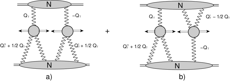
Figure 7: Mueller diagramsMUDI for the double inclusive cross section of pair $J/\Psi$ production.The wavy lines describe the BFKL Pomerons. The vertex V is defined in Eq. (15)

.4 Conclusions

In this letter we demonstrated that the two parton showers mechanism leads to much smaller values of $\sigma_{\rm eff}\leq 5\,mb$ for the double parton interaction. This result is in qualitative agreement with the data, and we consider it as support for the idea that the production of two parton showers is responsible for $J/\Psi$ inclusive cross section. The second result of this letter is the claim, that a simple two channel model with restrictions that stem from the results of the experiments on diffractive production in DIS, is able to describe the size of the double parton interaction at high energies leading to the values of $\sigma_{\rm eff}\leq 20\,mb$ for 4 jet production, in accord with the experimental data.

As has been mentioned above, the value of $\sigma_{\rm eff}$ is determined by the contribution of the long distances to the cross sections of hard processes. These contributions are doomed to be modeled at present time using the phenomenological input, since out knowledge of the non-perturbative QCD is still very limited.

Our numerical estimates are based on Eq. (13) and on the numerical values for the slopes $B_{el}$ and $B_{in}$. We checked that the smallness of $\sigma_{\rm eff}$ for $J/\Psi$ pair production has only a mild dependence on the value of $B_{in}$, which was measured with large errors. The two channel model has been used for describing the soft high energy dataGLP , It should be noted, that for the BFKL Pomeron, whose intercept is larger than 1, the integral over the produced mass in diffraction is convergent, and the Good-Walker mechanismGW is able to describe the diffractive production of both small and large massesGUGU . Therefore, we believe it reasonable to use this model to obtain the first estimates of the value of $\sigma_{\rm eff}$. It should be stressed that in the two channel model, that we used, the parameter $\alpha$ determines the structure of the wave function of the hadron, and does not depend on the processes under consideration.

Acknowledgements.
We thank all participants of Low-x 2019 WS and especially L. Motyka for encouraging discussions. This research was supported by CONICYT PIA/BASAL FB0821(Chile) and Fondecyt (Chile) grant 1180118 .

References

- (1) M. Diehl and J. R. Gaunt, “Double parton scattering theory overview,” Adv. Ser. Direct. High Energy Phys. 29 (2018) 7, [arXiv:1710.04408 [hep-ph]].
- (2) T. Akesson et al. [Axial Field Spectrometer Collaboration], “Double Parton Scattering in Collisions at -GeV,” Z. Phys. C 34, 163 (1987). doi:10.1007/BF01566757
- (3) J. Alitti et al. [UA2 Collaboration], “A Study of multi - jet events at the CERN anti-p p collider and a search for double parton scattering,” Phys. Lett. B 268, 145 (1991). doi:10.1016/0370-2693(91)90937-L
- (4) F. Abe et al. [CDF Collaboration], “Study of four jet events and evidence for double parton interactions in collisions at TeV,” Phys. Rev. D 47, 4857 (1993). doi:10.1103/PhysRevD.47.4857
- (5) F. Abe et al. [CDF Collaboration], “Double parton scattering in collisions at TeV,” Phys. Rev. D 56, 3811 (1997). doi:10.1103/PhysRevD.56.3811
- (6) V. M. Abazov et al. [D0 Collaboration], “Double parton interactions in +3 jet events in bar collisions TeV.,” Phys. Rev. D 81, 052012 (2010) doi:10.1103/PhysRevD.81.052012 [arXiv:0912.5104 [hep-ex]].
- (7) R. Aaij et al. [LHCb Collaboration], “Observation of double charm production involving open charm in pp collisions at = 7 TeV,” JHEP 1206, 141 (2012) Addendum: [JHEP 1403, 108 (2014)] doi:10.1007/JHEP03(2014)108, 10.1007/JHEP06(2012)141 [arXiv:1205.0975 [hep-ex]].
- (8) G. Aad et al. [ATLAS Collaboration], “Measurement of hard double-parton interactions in + 2 jet events at =7 TeV with the ATLAS detector,” New J. Phys. 15, 033038 (2013) doi:10.1088/1367-2630/15/3/033038 [arXiv:1301.6872 [hep-ex]].
- (9) S. Chatrchyan et al. [CMS Collaboration], “Study of double parton scattering using W + 2-jet events in proton-proton collisions at = 7 TeV,” JHEP 1403, 032 (2014) doi:10.1007/JHEP03(2014)032 [arXiv:1312.5729 [hep-ex]].
- (10) M. Aaboud et al. [ATLAS Collaboration], “Study of hard double-parton scattering in four-jet events in pp collisions at TeV with the ATLAS experiment,” JHEP 1611, 110 (2016) doi:10.1007/JHEP11(2016)110 [arXiv:1608.01857 [hep-ex]].
- (11) V. M. Abazov et al. [D0 Collaboration], “Double Parton Interactions in Jet and Jet Events in Collisions at TeV,” Phys. Rev. D 89, no. 7, 072006 (2014) doi:10.1103/PhysRevD.89.072006 [arXiv:1402.1550 [hep-ex]].
- (12) R. Aaij et al. [LHCb Collaboration], “Observation of double charm production involving open charm in pp collisions at = 7 TeV,” JHEP 1206, 141 (2012) Addendum: [JHEP 1403, 108 (2014)] doi:10.1007/JHEP03(2014)108, 10.1007/JHEP06(2012)141 [arXiv:1205.0975 [hep-ex]].
- (13) G. Aad et al. [ATLAS Collaboration], “Measurement of hard double-parton interactions in + 2 jet events at =7 TeV with the ATLAS detector,” New J. Phys. 15, 033038 (2013) doi:10.1088/1367-2630/15/3/033038 [arXiv:1301.6872 [hep-ex]].
- (14) S. Chatrchyan et al. [CMS Collaboration], “Study of double parton scattering using W + 2-jet events in proton-proton collisions at = 7 TeV,” JHEP 1403, 032 (2014) doi:10.1007/JHEP03(2014)032 [arXiv:1312.5729 [hep-ex]].
- (15) M. Aaboud et al. [ATLAS Collaboration], “Study of hard double-parton scattering in four-jet events in pp collisions at TeV with the ATLAS experiment,” JHEP 1611, 110 (2016) doi:10.1007/JHEP11(2016)110 [arXiv:1608.01857 [hep-ex]].
- (16) V. M. Abazov et al. [D0 Collaboration], “Double Parton Interactions in Jet and Jet Events in Collisions at TeV,” Phys. Rev. D 89, no. 7, 072006 (2014) doi:10.1103/PhysRevD.89.072006 [arXiv:1402.1550 [hep-ex]].
- (17) G. Aad et al. [ATLAS Collaboration], “Observation and measurements of the production of prompt and non-prompt mesons in association with a boson in collisions at = 8 TeV with the ATLAS detector,” Eur. Phys. J. C 75, no. 5, 229 (2015) doi:10.1140/epjc/s10052-015-3406-9 [arXiv:1412.6428 [hep-ex]].
- (18) R. Aaij et al. [LHCb Collaboration], “Production of associated Y and open charm hadrons in pp collisions at and 8 TeV via double parton scattering,” JHEP 1607, 052 (2016) doi:10.1007/JHEP07(2016)052 [arXiv:1510.05949 [hep-ex]].
- (19) V. M. Abazov et al. [D0 Collaboration], “Study of double parton interactions in diphoton + dijet events in collisions at TeV,” Phys. Rev. D 93, no. 5, 052008 (2016) doi:10.1103/PhysRevD.93.052008 [arXiv:1512.05291 [hep-ex]].
- (20) A. M. Sirunyan et al. [CMS Collaboration], “Constraints on the double-parton scattering cross section from same-sign W boson pair production in proton-proton collisions at TeV,” JHEP 1802, 032 (2018) doi:10.1007/JHEP02(2018)032 [arXiv:1712.02280 [hep-ex]].
- (21) M. Aaboud et al. [ATLAS Collaboration], “Study of the hard double-parton scattering contribution to inclusive four-lepton production in collisions at 8 TeV with the ATLAS detector,” Phys. Lett. B 790 (2019) 595 doi:10.1016/j.physletb.2019.01.062 [arXiv:1811.11094 [hep-ex]].
- (22) R. Aaij et al. [LHCb Collaboration], “Measurement of the J/ pair production cross-section in pp collisions at TeV,” JHEP 1706, 047 (2017) Erratum: [JHEP 1710, 068 (2017)] doi:10.1007/JHEP06(2017)047, 10.1007/JHEP10(2017)068 [arXiv:1612.07451 [hep-ex]].
- (23) V. M. Abazov et al. [D0 Collaboration], “Observation and Studies of Double Production at the Tevatron,” Phys. Rev. D 90, no. 11, 111101 (2014) doi:10.1103/PhysRevD.90.111101 [arXiv:1406.2380 [hep-ex]].
- (24) V. M. Abazov et al. [D0 Collaboration], “Evidence for simultaneous production of and mesons,” Phys. Rev. Lett. 116, no. 8, 082002 (2016) doi:10.1103/PhysRevLett.116.082002 [arXiv:1511.02428 [hep-ex]].
- (25) M. Aaboud et al. [ATLAS Collaboration], “Measurement of the prompt J/ pair production cross-section in pp collisions at TeV with the ATLAS detector,” Eur. Phys. J. C 77, no. 2, 76 (2017) doi:10.1140/epjc/s10052-017-4644-9 [arXiv:1612.02950 [hep-ex]].
- (26) V. Khachatryan et al. [CMS Collaboration], “Observation of (1S) pair production in proton-proton collisions at TeV,” JHEP 1705, 013 (2017) doi:10.1007/JHEP05(2017)013 [arXiv:1610.07095 [hep-ex]].
- (27) Y. V. Kovchegov and E. Levin“ Quantum chromodynamics at high energy" Vol. 33 (Cambridge University Press, 2012).
- (28) E. Levin and M. Siddikov, “ production in hadron scattering: three-pomeron contribution,” Eur. Phys. J. C 79 (2019) no.5, 376 doi:10.1140/epjc/s10052-019-6894-1 [arXiv:1812.06783 [hep-ph]].
- (29) A. H. Mueller, “O(2,1) ANALYSIS OF SINGLE PARTICLE SPECTRA AT HIGH-ENERGY,” Phys. Rev. D2 (1970) 2963.
- (30) V. S. Fadin, E. A. Kuraev and L. N. Lipatov, “On the pomeranchuk singularity in asymptotically free theories", Phys. Lett. B60, 50 (1975); E. A. Kuraev, L. N. Lipatov and V. S. Fadin, “The Pomeranchuk Singularity in Nonabelian Gauge Theories" Sov. Phys. JETP 45, 199 (1977), [Zh. Eksp. Teor. Fiz.72,377(1977)]; “The Pomeranchuk Singularity in Quantum Chromodynamics,” I. I. Balitsky and L. N. Lipatov, Sov. J. Nucl. Phys. 28, 822 (1978), [Yad. Fiz.28,1597(1978)].
- (31) L. N. Lipatov, “The Bare Pomeron in Quantum Chromodynamics,” Sov. Phys. JETP 63, 904 (1986) [Zh. Eksp. Teor. Fiz. 90, 1536 (1986)].
- (32) E. Levin and A. H. Rezaeian, “The Ridge from the BFKL evolution and beyond,” Phys. Rev. D 84 (2011) 034031 doi:10.1103/PhysRevD.84.034031 [arXiv:1105.3275 [hep-ph]].
- (33) C. Alexa et al. [H1 Collaboration], “Elastic and Proton-Dissociative Photoproduction of J/psi Mesons at HERA,” Eur. Phys. J. C 73, no. 6, 2466 (2013) doi:10.1140/epjc/s10052-013-2466-y [arXiv:1304.5162 [hep-ex]].
- (34) A. Aktas et al. [H1 Collaboration], “Elastic J/psi production at HERA,” Eur. Phys. J. C 46, 585 (2006) doi:10.1140/epjc/s2006-02519-5 [hep-ex/0510016].
- (35) S. Chekanov et al. [ZEUS Collaboration], “Exclusive electroproduction of J/psi mesons at HERA,” Nucl. Phys. B 695, 3 (2004) doi:10.1016/j.nuclphysb.2004.06.034 [hep-ex/0404008];Eur. Phys. J. C 24, 345 (2002) doi:10.1007/s10052-002-0953-7 [hep-ex/0201043].
- (36) E. Gotsman, E. Levin and I. Potashnikova, “CGC/saturation approach: soft interaction at the LHC energies,” Phys. Lett. B 781 (2018) 155, [arXiv:1712.06992 [hep-ph]].
- (37) M. L. Good and W. D. Walker,“Diffraction Dissociation of Beam Particles", Phys. Rev. 120 (1960) 1857.
- (38) G. Gustafson, “The Relation between the Good-Walker and Triple-Regge Formalisms for Diffractive Excitation,” Phys. Lett. B 718 (2013) 1054, [arXiv:1206.1733 [hep-ph]].