Information Gathering in Ad-Hoc Radio Networks

Abstract.

In the ad-hoc radio network model, nodes communicate with their neighbors via radio signals, without knowing the topology of the underlying digraph. We study the information gathering problem, where each node has a piece of information called a rumor, and the objective is to transmit all rumors to a designated target node. For the model without any collision detection we provide an ${\tilde{O}}(n^{1.5})$ deteministic protocol, significantly improving the trivial bound of $O(n^{2})$. We also consider a model with a mild form of collision detection, where a node receives a 1-bit acknowledgement if its transmission was received by at least one out-neighbor. For this model we give a ${\tilde{O}}(n)$ deterministic protocol for information gathering in acyclic graphs.

1. Introduction

We address the problem of information gathering in ad-hoc radio networks. A radio network is represented by a directed graph (digraph) $G$, whose nodes represent radio transmitters/receivers and directed edges represent their transmission ranges; that is, an edge $(u,v)$ is present in the digraph if and only if node $v$ is within the range of node $u$. When a node $u$ transmits a message, this message is immediately sent out to all its out-neighbors. However, a message may be prevented from reaching some out-neighbors of $u$ if it collides with messages from other nodes. A collision occurs at a node $v$ if two or more in-neighbors of $v$ transmit at the same time, in which case $v$ will not receive any of their messages, and it will not even know that they transmitted.

Radio networks, as defined above, constitute a useful abstract model for studying protocols for information dissemination in networks where communication is achieved via broadcast channels, as opposed to one-to-one links. Such networks do not need to necessarily utilize radio technology; for example, in local area networks based on the ethernet protocol all nodes communicate by broadcasting information through a shared carrier. Different variants of this model have been considered in the literature, depending on the assumptions about the node labels (that is, identifiers), on the knowledge of the underlying topology, and on allowed message size. In this work we assume that nodes are labelled $0,1,...,n-1$, where $n$ is the network size. (All our results remain valid if the labels are selected from the range $0,1,...,O(n)$.) We focus on the ad-hoc model, where the digraph’s topology is uknown when the computation starts, and a protocol needs to complete its task within a desired time bound, no matter what the topology is. At the beginning of the computation each node $v$ is in possession of a unique piece of information, that we refer to as a rumor. Different communication primitives are defined by specifying how these rumors need to be disseminated across the network. In this paper we do not make any assumptions about the size of transmitted messages; thus a node can aggregate multiple rumors and transmit them in one message. In fact, it could as well transmit as one message the complete history of its past computation.

Two most studied information dissemination primitives for this model are broadcasting and gossiping. In broadcasting (or one-to-all communication), a single source node $s$ attempts to deliver its rumor to all nodes in the network. For broadcasting to be meaningful, we need to assume that all nodes in $G$ are reachable from $s$. In gossiping (or all-to-all communication), the objective is to distribute all rumors to all nodes in the network, under the assumption that $G$ is strongly connected. Both these primitives can be solved in time $O(n^{2})$ by a simple protocol called RoundRobin where all nodes transmit cyclically one at a time (see Section 2). Past research on ad-hoc radio networks focussed on designing protocols that improve this trivial bound.

For broadcasting, gradual improvements in the running time have been reported since early 2000’s  [6, 20, 2, 3, 12, 11], culminating in the upper bound of $O(n\log D\log\log(D\Delta/n))$ in [10], where $D$ denotes the diameter of $G$ and $\Delta$ its maximum in-degree. This is already almost tight, as the lower bound of $\Omega(n\log D)$ is known [9]. For randomized algorithms, the gap between lower and upper bounds is also almost completely closed, see [1, 21, 11].

In case of gossiping, major open problems remain. The upper bound of $O(n^{2})$ was improved to ${\tilde{O}}(n^{1.5})$ in [6, 26] and then later to ${\tilde{O}}(n^{4/3})$ in [17], and no better bound is currently known. No lower bound better than $\Omega(n\log n)$ (that follows from [9]) is known. In contrast, in the randomized case it is possible to achieve gossiping in time ${\tilde{O}}(n)$ [11, 22, 7].

The reader is referred to survey papers [14, 19, 15, 25, 18] that contain more information about information dissemination protocols in different variants of radio networks.

In this paper we address the problem of information gathering (that is, all-to-one communication). In this problem, similar to gossiping, each node $v$ has its own rumor, and the objective is to deliver these rumors to a designated target node $t$. (We assume that $t$ is reachable from all nodes in $G$.)

The problem of information gathering for trees was introduced in [5], where an $O(n)$-time algorithm was presented. Other results in [5] include algorithms for the model without rumor aggregation or the model with transmission acknowledgements.

Our results. Our main result, in Section 4, is a deterministic protocol that solves the information gathering problem in arbitrary ad-hoc networks in time ${\tilde{O}}(n^{1.5})$. To our knowledge this is the first such a protocol that achieves running time faster than the trivial $O(n^{2})$ bound. One of our key technical contributions is in solving this problem in time ${\tilde{O}}(n^{1.5})$ for acyclic graphs (Section 3) where any protocols developed earlier for gossiping, that rely on feedback (see the discussion below), are not applicable. This algorithm for acyclic graphs is based on careful application of combinatorial structures called strong selectors, combined with a novel amortization technique to measure progress of the algorithm. To extend this protocol to arbitrary graphs, we integrate it with a gossiping protocol. Roughly, the two sub-protocols run in parallel, with the sub-protocol for acyclic graphs transferring information between strongly connected components, while the gossiping sub-protocol disseminates it within each strongly connected component. This requires overcoming two challenges. One is that the partition of $G$ into strongly connected components is not actually known, so the combined protocol needs to gradually “learn” the connectivity structure of $G$ while it executes. The second challenges is in synchronizing the computation of the two sub-protocols, since they are based on entirely different principles.

In the second part of the paper, in Section 5, we consider a slight relaxation of our model by allowing a mild form of collision detection. In this new model each node $v$, after each transmission, receives a 1-bit acknowledgement indicating whether its transmission was received by at least one out-neighbor. With this assumption, we provide an ${\tilde{O}}(n)$-time algorithm for information dissemination in acyclic radio networks.

Additional context and motivations. If $G$ is strongly connected then information gathering and gossiping are equivalent. Trivially, a gossiping algorithm gathers all rumors in $t$, solving the information gathering problem. On the other hand, one can solve the gossiping problem by running an information gathering protocol followed by any ${\tilde{O}}(n)$-time broadcasting protocol with source node $t$. Thus, counter-intuitively, information gathering can be thought of as an extension of gossiping, since it applies to a broader class of graphs.

The crucial challenge in designing protocols for information gathering is lack of feedback, namely that the nodes in the network do not receive any information about the fate of their transmissions. This should be contrasted with the gossiping problem where, due to the assumption of strong connectivity, a node can eventually learn whether its earlier transmissions were successful. In fact, the existing protocols for gossiping critically rely on this feature, as they use it to identify nodes that have collected a large number of rumors, and then they broadcast these rumors to the whole network, thus removing them from consideration and reducing congestion.

Some evidence that feedback might help to speed up information gathering can be found in [4], where the authors developed an $O(n)$-time protocol for trees if nodes receive (immediate) acknowledgements of successful transmissions, while the best known upper bound for this problem without feedback is $O(n\log\log n)$.

Various forms of feedback have been studied in the past in the context of contention resolution for multiple-access channels (MAC), where nodes communicate via a single shared challel. (Ethernet is one example.) Depending on more specific characteristics of this shared channel, one can model this problem as the information gathering problem either on a complete graph or a star graph, which is a collection of $n$ nodes connected by directed edges to the target node $t$. (See [23, 24, 13] for information about contention resolution protocols.) For instance, in [5] a tight bound of $\Theta(n\log n)$ was given for randomized information gathering on star graphs (or MACs) even if the nodes have no labels (are indistinguishable) and receive no feedback.

As explained earlier, in our model rumor aggregation is allowed. This capability is needed to beat the $O(n^{2})$ upper bound, as without rumor aggregation it is quite easy to show a lower bound of $\Omega(n^{2})$ for both gossiping and information gathering, and even for randomized algorithms and with the topology known [16].

Interestingly, if we allow randomization, the randomized gossiping algorithms in [7, 22] can be adapted to information gathering without increasing the running time. Thus randomization can not only help to overcome collisions, but also lack of feedback.

2. Preliminaries

Graph terminology. Throughout the paper, we assume that the radio network is represented by a digraph (directed graph) $G$ with a distinguished target node $t$ that is reachable from all other nodes. By $n=|G|$ we denote the number of nodes in $G$. We will treat $G$ both as a set of vertices and edges, and write $u\in G$ if $u$ is a node of $G$ and $(u,v)\in G$ if $(u,v)$ is an edge of $G$. If $(u,v)\in G$ then we refer to $u$ as the in-neighbor of $v$ and to $v$ as the out-neighbor of $u$. For any node $v$, by ${N^{-}}(v)={\left\{u\in G{\;:\;}(u,v)\in G\right\}}$ we denote the set of its in-neighbors.

For brevity, we will refer to strongly connected components of $G$ as sc-components. For each node $v$, the sc-component containing $v$ will be denoted by ${C}(v)$. We partition the set of in-neighbors of $v$ into those that belong to ${C}(v)$ and those that do not: ${N^{-}_{\scriptscriptstyle\textrm{scc}}}(v)={N^{-}}(v)\cap{C}(v)$ and ${N^{-}_{\scriptscriptstyle\textrm{acy}}}(v)={N^{-}}(v)\setminus{C}(v)$.

The in-graph of $v$ in $G$, denoted $G^{-}(v)$, is the set of all nodes of $G$ from which $v$ is reachable (via a directed path). We extend this definition in a natural way to sc-components of $G$; if $A$ is an sc-component then its in-graph is $G^{-}(A)=\bigcup_{v\in A}G^{-}(v)$.

Radio networks. As mentioned in the introduction we assume that each node of $G$ has a unique label from the set ${\left[n\right]}={\left\{0,1,...,n-1\right\}}$. For convenience, we will identify nodes with their labels, so a “node $u$” really means the node with label $u$.

The time is divided into discrete time steps numbered with non-negative integers. We assume that all nodes start to execute the protocol simultaneously at time step $0$. In the formal model of radio networks, at each step each node can be either in a transmitting state, when it can transmit a message, or receiving state, when it can only listen to transmissions from other nodes. We will show below, however, that we can relax these restrictions and allow a node to simultaneously listen and transmit at each step. Only one message can be transmitted at each step. This is not an essential restriction because, as already mentioned, we are not imposing any restrictions on the size or format of messages transmitted by nodes. However, a message transmited at a given step cannot depend on the message (if any) received in the same step.

If a node $u$ transmits a message at a time $\tau$, this message reaches all out-neighbors of $u$ in the same step. If $v$ is one of these out-neighbors, and if $u$ is the only in-neighor of $v$ that transmits at time $\tau$, then $v$ will receive this message. However, if there are two or more in-neighbors of $v$ that transmit at time $\tau$ then a collision occurs, and $v$ does not receive any information. In other words, collisions are indistinguishable from absence of transmissions. There is no feedback mechanism available in this model, that is a sender of a message does not receive any information as to whether its transmission was successful or not. (We will relax this restriction later in Section 5.)

Selectors. A strong $(n,k)$-selector is a sequence of label sets $(S_{0},S_{1},...,S_{\ell-1})$ (that is, $S_{i}\subseteq[n]$ for each $i$) that “singles out” each label from each subset of at most $k$ labels, in the following sense: for each $X\subseteq{\left[n\right]}$ with $|X|\leq k$ and each $x\in X$ there is an index $i$ such that $S_{i}\cap X={\left\{x\right\}}$. It is known [8] that there exist strong $(n,k)$-selectors of size $\ell=O(k^{2}\log n)$.

Such selectors are often used for designing protocols for ad-hoc radio networks. The intuition is this: Consider a protocol that cyclically “runs” a strong $(n,k)$-selector; that is, each node $w$ transmits in a step $\tau$ if and only if $w\in S_{\tau\bmod\ell}$. Suppose that $u$ starts transmitting its message at some time step and then follows this protocol. If $v$ is an out-neighbor of $u$ and $v$’s in-degree is at most $k$, then $v$ will successfully receive $u$’s message in at most $O(k^{2}\log n)$ steps, independently of the label assignment. Another basic protocol that is often used is called RoundRobin. In this protocol all nodes transmit cyclically one by one; that is each node $w$ transmits in a step $\tau$ if and only if $w=\tau\bmod n$. In RoundRobin there are no collisions so, in the setting above, node $u$ will successfully transmit its message to $v$ in at most $n$ time steps. Note that a protocol based on a strong $(n,k)$-selector can be faster than RoundRobin only when $k=O(\sqrt{n/\log n})$.

For all $j=0,1,...,{\textstyle\frac{1}{2}}\log n$, by ${\textsc{$2^{j}$-Select}}=(S^{j}_{0},S^{j}_{1},...,S^{j}_{\ell_{j}-1})$ we will denote a strong $(n,2^{j})$-selector of size $\ell_{j}=O(4^{j}\log n)$. Without loss of generality we can assume that $\ell_{j+1}=4\ell_{j}$ for all $j\leq{\textstyle\frac{1}{2}}\log n-1$.

Note: To avoid clutter, in the paragraph above, as well as later throughout the paper, we omit the notation for rounding and assume that in all formulas representing integer quantities (the number of nodes, steps, etc.) their values are appropriately rounded. This will not affect asymptotic running time estimates.

In Section 5, where we consider transmissions with acknowledgements, it will be desirable to have many (but not necessarily all) of a collection of competing in-neighbors of a node transmit successfully. For this purpose we will there introduce a different type of selectors.

Simplifying assumptions. To streamline the description of our algorithms, in the paper we will assume a relaxed communication model with two additional features:

:

(MFC) We assume that some number $\kappa$ of radio frequency channels, numbered $0,1,...,\kappa-1$, is available for communication. In a single step, a node can use all frequencies simultaneously.

:

(SRT) Further, for each frequency $f$, a node can receive and transmit at frequency $f$ in a single step. The restriction is that the messages transmitted at all frequencies in any step do not depend on the messages received in this step.

Below we explain how this relaxed model can be simulated using the standard radio network model, increasing the running time by factor $O(\kappa)$; that is, any protocol that uses features (MFC) and (SRT) and runs in time $O(T)$ can be converted into a protocol in the standard model whose running time is $O(\kappa T)$. Since $\kappa=O(\log n)$ in our protocols, their ${\tilde{O}}(\cdot)$-complexity is not affected.

Simulating multiple frequencies. We first explain how we can convert a protocol ${\cal A}$ that uses $\kappa$ frequencies and runs in time $O(T)$ into a protocol ${\cal A}^{\prime}$ that uses only one frequency and runs in time $O(\kappa T$). This can be done by straightforward time multiplexing. In more detail: ${\cal A}^{\prime}$ organizes all time steps $0,1,2,...$ into rounds. Each round $r=0,1,2,...$ consists of $\kappa$ consecutive steps $r\kappa,r\kappa+1,...,r\kappa+\kappa-1$. Each step $s$ of ${\cal A}$ is simulated by round $s$ of ${\cal A}^{\prime}$. For each frequency $f$, the message transmitted at frequency $f$ by ${\cal A}$ is transmitted by ${\cal A}^{\prime}$ in step $s\kappa+f$, that is the $f$th step of round $s$. At the end of round $s$, ${\cal A}^{\prime}$ will know all messages received in this round, so it will know what messages would ${\cal A}$ receive in step $s$, and therefore it knows the state of ${\cal A}$ and can determine the transmissions of $A$ in the next step.

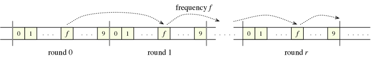
Figure 1. Partition of ${\cal A}^{\prime}$’s time steps into rounds, for $\kappa=10$ frequencies.

Simulating simultaneous receiving/transmitting. By the argument above, we can assume that we have only one frequency channel. We claim that we can disallow simultaneous receiving and transmitting at the cost of only adding a logarithmic factor to the running time. To see this, suppose that ${\cal B}$ is some transmission protocol where nodes can transmit and listen at the same time. (Recall that the transmission of ${\cal B}$ at any step does not depend on the information it receives in the same step.) We use a strong $(n,2)$-selector ${\textsc{$2$-Select}}=(S^{1}_{i})_{i}$ of size $\ell_{1}={\tilde{O}}(1)$. We replace each step $\tau$ of ${\cal B}$ by a time segment $I_{\tau}$ of length $\ell_{1}$. For any node $u$ and any $i=0,1,...,|I_{\tau}|-1$, if $v\in S^{1}_{i}$ then at the $i$th step of segment $I_{\tau}$ node $v$ transmits whatever message it would transmit in ${\cal B}$ at time $\tau$; otherwise $v$ is in the receiving state. By definition, in this new protocol ${\cal B}^{\prime}$ nodes do not transmit and receive at the same time. Further, for any edge $(u,v)$, if $u$ transmitted successfully to $v$ in step $\tau$ of ${\cal B}$, in ${\cal B}^{\prime}$ there will be a time step within $I_{\tau}$ at which $u$ is in the transmitting state and $v$ is in the receiving state, guaranteeing that $u$’s message will reach $v$.

In fact, for the type of protocols presented in the paper, allowing simultaneous reception and transmisison does not affect the asymptotic running time at all. Our protocols are based on strong selectors and RoundRobin. In case of RoundRobin, the simultaneous reception and transmisison capability is (trivially) not needed. For selector-based protocols, the argument how this capability can be removed was given in [4]. Roughly, the idea is that whenever a protocol uses a strong $(n,k)$-selector, this selector can be replaced by a strong $(n,k+1)$-selector (whose size is asymptotically the same). This guarantees that, during each complete cycle (of length $O(k^{2}\log n)$) of this selector, for any node $v$ with $k$ in-neighbors and any $v$’s in-neighbor $u$ there will be a step when $v$ is in the receiving state and $u$ is the only in-neighbor in the transmitting state.

3. ${\tilde{O}}(n^{1.5})$-Time Protocol for Acyclic Digraphs

We first consider ad-hoc radio networks whose underlying digraph $G$ is acyclic and has one designated target node $t$ that is reachable from all other nodes in $G$. We give a deterministic information gathering protocol that gathers all rumors in the target node $t$ in time ${\tilde{O}}(n^{1.5})$, independently of the topology of $G$.

In the algorithm we will assume that each vertex knows the labels of its in-neighbors. This can be easily achieved in time $O(n)$ by pre-processing that consists of one cycle of RoundRobin, where each node transmits only its own label. As explained in Section 2, we also make Assumptions (MFC) and (SRT), namely that the protocol has multiple frequency channels available and on each frequency it can simultaneously receive and transmit messages at each step.

Let $\theta={\textstyle\frac{1}{2}}(\log n-\log\log n)+2$. In the algorithm below we use a sequence of $\theta+1$ values $\beta_{0},\beta_{1},...,\beta_{\theta}$, defined as follows: $\beta_{0}=0$, $\beta_{j}=\sum_{g<j}\ell_{g}$ for $j=1,...,\theta-1$, and $\beta_{\theta}=\sum_{g<\theta}\ell_{g}+n$.

Protocol AcyGather. The algorithm uses $\theta$ frequencies numbered $0,1,...,\theta-1$. The intuition is that each frequency $j\leq\theta-2$ will be used to run selector $2^{j}$-Select, while frequency $\theta-1$ will be used to run RoundRobin.

At each step, a node could be dormant or active. Dormant nodes do not transmit; active nodes may or may not transmit. A node $v$ is active during its activity period $[\alpha(v),\alpha(v)+\beta_{\theta})$, where $\alpha(v)$ is referred to as the activation step of $v$, and is defined below.

If $v$ is a source node (that is, its in-degree is $0$), then $\alpha(v)=0$. Otherwise $\alpha(v)$ is determined by the messages received by $v$, as follows. Each message transmitted by a node $u$ contains the following information: (i) all rumors collected by $u$, including its own, (ii) the label of $u$, and (iii) another value called recommended wake-up step and denoted ${\textit{rws}}_{u}$, to be defined shortly. For a non-source node $v$ and its in-neighbor $u$, denote by ${\textit{rws}}^{1}_{u,v}$ the first ${\textit{rws}}_{u}$ value received by $v$ from $u$. (This may not be the first ${\textit{rws}}_{u}$ value transmitted by $u$, since earlier transmissions of $u$ might have collided at $v$.) Node $v$ waits until it receives messages from all its in-neighbors, and, as soon as this happens, if $u$ is the last in-neighbor of $v$ that successfully transmitted to $v$, then $v$ sets $\alpha(v)={\textit{rws}}^{1}_{u,v}$. (Occasionally we will write ${\textit{rws}}^{1}(u,v)$ instead of ${\textit{rws}}^{1}_{u,v}$, to avoid multi-level indexing.)

The activity period $[\alpha(v),\alpha(v)+\beta_{\theta})$ of $v$ is divided into $\theta$ activity stages, where, for $j=0,1,...,\theta-1$, the $j$th activity stage consists of the time interval $[\alpha(v)+\beta_{j},\alpha(v)+\beta_{j+1})$. (See Figure 2.) During its $j$th activity stage, for $j\leq\theta-2$, node $v$ transmits according to selector $2^{j}$-Select using frequency $j$. During the $(\theta-1)$th activity stage, the protocol transmits using RoundRobin on frequency $\theta-1$. The recommended wake-up step value included in $v$’s messages during its $j$th activity stage is ${\textit{rws}}_{v}=\alpha(v)+\beta_{j+1}$. At all other times $v$ does not transmit.

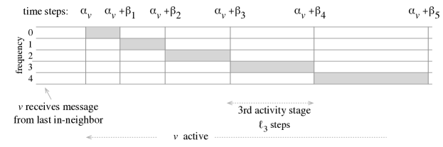
Figure 2. Illustration of activity stages. (The picture is not up to scale. In reality the length of activity stages increases at rate $4$.) Shaded regions show frequencies used in different activity stages.

Correctness. We first note that the algorithm is correct, in the sense that each rumor will eventually reach the target node $t$. This is true because once a node becomes active, it is guaranteed to successfully transmit its message to its all out-neighbors using the RoundRobin protocol during its last activity stage.

Running time. Next, we show that Protocol AcyGather completes information gathering in time ${\tilde{O}}(n^{1.5})$. To establish this bound, we choose in the graph $G$ a critical path $P=(v_{0},v_{1},...,v_{p}=t)$, defined as follows: for each $a=p-1,p-2,...,0$, $v_{a}$ is the in-neighbor of $v_{a+1}$ who was last to successfully transmit to $v_{a+1}$ (thus $\alpha(v_{a+1})={\textit{rws}}^{1}_{v_{a},v_{a+1}}$), and $v_{0}$ is a source node. (Note that, since we define this path in the backwards order, the indexing of the nodes $v_{a}$ can be determined only after we determine the whole path). The overall running time is upper-bounded by the time for the rumor of $v_{0}$ to reach $t$ along $P$.

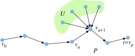
Figure 3. Illustration of the time analysis for acyclic graphs.

If at a step $\tau$ a node $v$ is in its $j$-th activity stage (that is, $\tau\in[\alpha(v)+\beta_{j},\alpha(v)+\beta_{j+1})$) then we refer to $j$ as $v$’s stage index in step $\tau$. We extend this (artificially) to dormant nodes as follows: if $v$ has not yet started its activity period then its stage index is $-1$, and if $v$ has already completed its activity period then its stage index is $\theta$. The stage index of each node is incremented $\theta+1=O(\log n)$ times, so the total number of these increments, over all nodes and over the whole computation, is $O(n\log n)={\tilde{O}}(n)$.

Now consider some node $v_{a}$ on $P$. (See Figure 3.) Our argument is based on the following key lemma.

Lemma 3.1.

There are ${\tilde{\Omega}}(n^{-1/2}(\,\alpha(v_{a+1})-\alpha(v_{a})\,))$ stage index increments in the time interval $[\alpha(v_{a}),\alpha(v_{a+1}))$.

Before we prove Lemma 3.1, we argue that this lemma is sufficient to establish our ${\tilde{O}}(n^{1.5})$ upper bound. Let $T$ be the running time of Protocol AcyGather. Since $\alpha(v_{0})=0$ and $T\leq\alpha(v_{p})$, we can bound the running time as $T\leq\sum_{a=0}^{p-1}(\alpha(v_{a+1})-\alpha(v_{a}))$. Then Lemma 3.1 implies that the total number of stage index increments during the computation is ${\tilde{\Omega}}(n^{-1/2}T)$. Since this number is also ${\tilde{O}}(n)$, it gives us that $T={\tilde{O}}(n^{1.5})$.

Proof 3.2.

We now prove Lemma 3.1. Suppose that $v_{a}$ succeeds first time in transmitting its message to $v_{a+1}$ during its $h$-th activity stage.

Claim 1.

For $a<p$ and $h<\theta-1$ we have $\alpha(v_{a+1})-\alpha(v_{a})={\tilde{O}}(4^{h})$.

This claim follows from the definition of $P$, as $\alpha(v_{a+1})={\textit{rws}}^{1}_{v_{a},v_{a+1}}=\alpha(v_{a})+\beta_{h+1}$, and $\beta_{h+1}=\sum_{g<h}\ell_{g}=O(4^{h}\log n)$.

We now consider three cases, depending on the value of $h$. First, if $h=0$, then there is at least one stage increment in $[\alpha(v_{a}),\alpha(v_{a+1}))$ (namely the increment of the stage index of $v_{a}$ from $-1$ to $0$) and $\alpha(v_{a+1})-\alpha(v_{a})=\ell_{0}=O(\log n)$, so the lemma holds trivially.

Next, suppose that $1\leq h\leq\theta-2$. By the choice of $h$, $v_{a}$ has not succeeded in its $(h-1)$th activity stage $[\alpha(v_{a})+\beta_{h-1},\alpha(v_{a})+\beta_{h})$. Let $U$ be the set of in-neighbors of $v_{a+1}$ (including $v_{a}$) whose $(h-1)$th activity stage overlapped that of $v_{a}$.

Claim 2.

$|U|>2^{h-1}$.

To justify Claim 2, we argue by contradiction. Suppose that $|U|\leq 2^{h-1}$. During this activity stage $v_{a}$ transmitted according to $2^{h-1}$-Select using only frequency $h-1$. Further, by the definition of the protocol, at each step of this stage the in-neighbors of $v_{a+1}$ with stage index other than $h-1$ did not use frequency $h-1$ for transmissions. So the transmissions from $v_{a}$ to $v_{a+1}$ in this stage can only conflict with transmissions from $U\setminus{\left\{v_{a}\right\}}$ to $v_{a+1}$. The definition of strong selectors and the assumption that $|U|\leq 2^{h-1}$ imply that then $v_{a}$ would have successfully transmitted to $v_{a+1}$ during its $(h-1)$th activity stage, contradicting the definition of $h$. Thus Claim 2 is indeed true.

The $(h-1)$th activity stage lasts $\ell_{h-1}$ steps so all the $(h-1)$th activity stages of the nodes in $U$ end before time $\alpha(v_{a})+\beta_{h}+\ell_{h-1}<\alpha(v_{a})+\beta_{h+1}=\alpha(v_{a+1})$. This implies that in the interval $[\alpha(v_{a}),\alpha(v_{a+1}))$ the number of stage index increments is at least

$$|U|\;\geq\;2^{h-1}\;=\;{\textstyle\frac{1}{2}}\cdot 2^{-h}\cdot 4^{h}\;=\;{\tilde{\Omega}}(n^{-1/2}(\alpha(v_{a+1})-\alpha(v_{a}))),$$

because $h\leq{\textstyle\frac{1}{2}}\log n$ and $\alpha(v_{a+1})-\alpha(v_{a})={\tilde{O}}(4^{h})$. This completes the proof of the lemma when $1\leq h\leq\theta-2$.

Finally, consider the case when $h=\theta-1$. Then $\alpha(v_{a+1})-\alpha(v_{a})=n$. But, by the choice of $h$, $v_{a}$ has not succeeded in its $(h-1)$th activity stage, where $h-1={\textstyle\frac{1}{2}}(\log n-\log\log n)$. A similar argument as above gives us that the number of stage index increments during $v_{a}$’s $(h-1)$th activity stage is ${\tilde{\Omega}}(n^{1/2})$, implying Lemma 3.1.

More precise time bound. We have established that Algorithm AcyGather runs in time ${\tilde{O}}(n^{1.5})$ on acyclic graphs. For a more precise bound, let us now determine the exponent of the logarithmic factor in this bound: one factor $O(\log n)$ is needed to simulate multiple frequencies with one, one factor $O(\log n)$ appears in the bound for the length of selectors, and we have another factor $O(\log n)$ that we ignored in the amortized analysis, since the number of stage index increments is $O(n\log n)$ (while we used the bound of ${\tilde{O}}(n)$). This gives us the main result of this section:

Theorem 3.3.

Let $G$ be an acyclic directed graph with $n$ vertices and a designated target node reachable from all other nodes. Algorithm AcyGather completes information gathering on $G$ in time $O(n^{1.5}\log^{3}n)$.

4. ${\tilde{O}}(n^{1.5})$-Time Protocol for Arbitrary Digraphs

We now extend our information gathering protocol AcyGather from Section 3 to arbitrary digraphs, retaining running time ${\tilde{O}}(n^{1.5})$. Throughout this section $G$ will denote an $n$-vertex digraph with a designated target node $t$ that is reachable from all other nodes in $G$.

The main obstacle we need to overcome is that protocol AcyGather critically depends on on $G$ being acyclic. For instance, in that protocol each node waits until it receives messages from all its in-neighbors. If cycles are present in $G$, this leads to a deadlock, where each node in a cycle waits for its predecessor. On the other hand, the known gossiping protocols [6, 26, 17] do not work correctly if the graph is not strongly connected, because they rely on broadcasting to periodically flush out some rumors from the system and on leader election to synchronize computation.

The idea behind our solution is to integrate protocol AcyGather with the gossiping protocol from [17], using AcyGather to transmit information between different sc-components of $G$ and using gossiping to disseminate information within sc-components. The idea is natural but it faces several technical challenges. One challenge is that the sc-components of $G$ are actually not known. In fact, a node $v$ doesn’t even know the size of ${C}(v)$, but it needs to provide this size to the gossiping protocol. To get around this issue, $v$ runs in parallel $O(\log n)$ copies of a gossiping protocol for sizes that are powers of $2$. One other challenge is that $v$ needs to be able to determine whether at least one of these parallel gossiping protocols successfully completed. To achieve this, these gossiping protocols, in addition to rumors, distribute additional information about the node labels and their in-neighbors.

Protocol SccGossip for gossiping. We will refer to the gossiping algorithm from [17] as SccGossip. The following property of SccGossip is crucial for our algorithm:

:

(scc) If the input digraph is strongly connected and has at most $k$ vertices, with the node labels from the set $[K]={\left\{0,1,...,K-1\right\}}$, then algorithm SccGossip completes gossiping in time $O(k^{4/3}\log K\log^{7/3}k)$.

As explained earlier, one idea of our algorithm is to execute SccGossip on its sc-components. The details of this will be provided shortly. For now, we only make an observation that captures one basic principle of this process. Let $A$ be an sc-component of size $n_{A}$ and let $j$ be such that $2^{j-1}<n_{A}\leq 2^{j}$. Let ${{\textsc{SccGossip}}}_{j}$ denote SccGossip specialized for strongly connected digraphs of size $2^{j}$ and label set $[n]$, and let $T_{\scriptscriptstyle\textrm{SCC}}(j)$ be the running time of ${{\textsc{SccGossip}}}_{j}$ on such digraphs. Suppose also that all nodes in $G^{-}(A)\setminus A$ are dormant and that the nodes in $A$ execute ${{\textsc{SccGossip}}}_{j}$, all starting at the same time. Since there is no interference from outside $A$, using property (scc) with $k=2^{j}$ and $K=n$, this execution of ${{\textsc{SccGossip}}}_{j}$ will complete correctly in the subgraph of $G$ induced by $A$ in time $T_{\scriptscriptstyle\textrm{SCC}}(j)={\tilde{O}}(n_{A}^{4/3})$.

Algorithm ArbGather. Our protocol can be thought of as running two parallel subroutines, the SCC-subroutine and the ACY-subroutine, that use two disjoint sets of frequencies. There will be $\theta$ ACY-frequencies indexed $0,1,...,\theta-1$, where $\theta={\textstyle\frac{1}{2}}(\log n-\log\log n)+2$, as in Section 3. These will be used by the ACY-subroutine to simulate protocol AcyGather. We will also have $\theta^{\prime}=\log n$ SCC-frequencies indexed $0,1,...,\theta^{\prime}-1$, used by the SCC-subroutine to simulate protocol SccGossip. Due to using different frequencies, there will be no signal interference betweeen these two subroutines.

The SCC-subroutine. This subroutine uses the SCC-frequencies, with the SCC-frequency $j$ used to simulate protocol ${{\textsc{SccGossip}}}_{j}$, for $j=0,1,...,\theta^{\prime}-1$. For each SCC-frequency $j$, any node $v$ divides its time steps into $j$-frames, where the $s$-th $j$-frame, for $s=0,1,...$, is $[sT_{\scriptscriptstyle\textrm{SCC}}(j),(s+1)T_{\scriptscriptstyle\textrm{SCC}}(j))$ — an interval sufficient for a complete simulation (described below) of ${{\textsc{SccGossip}}}_{j}$ on a digraph with $2^{j}$ nodes. For each $j$, these simulations start at time $0$ and continue until $v$ determines that for at least one frequency $j^{\prime}$ some simulation successfully completed in ${C}(v)$.

The overall goal of $v$ executing its SCC-subroutine is to determine ${C}(v)$ and collect all rumors from it. The challenge is that, while $v$ executes its SCC-subroutine, it may be receiving messages from its in-neighbors in preceding sc-components, thus from outside ${C}(v)$. These messages are of two types: “good” messages received on ACY-frequencies, that contain rumors from the in-graph of $v$ and do not interfere with the SCC-subroutine in $v$, and “bad” messages received on SCC-frequencies that can cause the SCC-subroutine in $v$ to fail.

We now describe $v$’s simulation of ${{\textsc{SccGossip}}}_{j}$ on frequency $j$. The purpose of this simulation is two-fold: one, to determine ${C}(v)$, and two, to distribute all rumors already gathered in $v$ to all nodes in ${C}(v)$. This is done in two consecutive $j$-frames. For each $r=0,1,...$, in the $2r$-th $j$-frame $v$ executes ${{\textsc{SccGossip}}}_{j}$, using its own label $v$ as the “rumor” for the purpose of gossiping. Let ${{\tilde{C}}}(v)$ denote the set of labels received by $v$ during this $j$-frame, including $v$ itself. In the $(2r+1)$-th $j$-frame, $v$ again executes ${{\textsc{SccGossip}}}_{j}$, but this time its “rumor” is the vector $[v,{{\tilde{C}}}(v),{N^{-}}(v),{{{\tilde{N}}}^{-}_{\scriptscriptstyle\textrm{acy}}}(v),R(v)]$, where ${{{\tilde{N}}}^{-}_{\scriptscriptstyle\textrm{acy}}}(v)\subseteq{N^{-}}(v)$ is the set of in-neighbors of $v$ that have transmitted a message to $v$ on some ACY-frequency (and thus are in a preceding sc-component) before time $2rT_{\scriptscriptstyle\textrm{SCC}}(j)$, and $R(v)$ is the set of all (original) rumors received on ACY-frequencies before time $2rT_{\scriptscriptstyle\textrm{SCC}}(j)$, plus the rumor of $v$. (Recall that time step $2rT_{\scriptscriptstyle\textrm{SCC}}(j)$ is the beginning of $2r$-th $j$-frame.) Let ${{\tilde{C}}}^{\prime}(v)$ be the set of node labels received in the $(2r+1)$-th $j$-frame. Then, right after the $(2r+1)$th $j$-frame, $v$ performs three tests:

:

Test 1: Is it true that ${{\tilde{C}}}(v)={{\tilde{C}}}(u)$ for all $u\in{{\tilde{C}}}(v)$?

:

Test 2: Is it true that ${{\tilde{C}}}(v)={{\tilde{C}}}^{\prime}(v)$?

:

Test 3: Is it true that ${N^{-}}(u)\setminus{{{\tilde{N}}}^{-}_{\scriptscriptstyle\textrm{acy}}}(u)\subseteq{{\tilde{C}}}(v)$ for all $u\in{{\tilde{C}}}(v)$?

If one of these tests fails, $v$ continues the execution of the SCC-subroutine. If all tests pass, $v$ aborts its SCC-subroutine, discontinues using all SCC-frequencies, and switches to the AcyGather subroutine, with its set of collected rumors being $\bigcup_{u\in{{\tilde{C}}}(v)}R(u)$.

Unlike in AcyGather, with each node $v$ we now associate two activation times. The first one is called $v$’s SCC-activation and is defined analogously to the activation time in AcyGather: If ${N^{-}_{\scriptscriptstyle\textrm{acy}}}(v)=\emptyset$ then $\alpha_{\scriptscriptstyle\textrm{scc}}(v)=0$. Otherwise, $\alpha_{\scriptscriptstyle\textrm{scc}}(v)$ is the last-received value ${\textit{rws}}^{1}(u,v)$ for $u\in{N^{-}_{\scriptscriptstyle\textrm{acy}}}(v)$, where ${\textit{rws}}^{1}_{u,v}$ denotes the first ${\textit{rws}}_{u}$ value received by $v$ from $u$. As explained earlier, these values will be received on the ACY-frequency. (Note that the algorithm does not actually use SCC-activation values for computation — these will be used only for the analysis.) If $r$ is the index such that Tests 1 and 2 pass after the double $j$-frames $2r$ and $2r+1$ then the second activation time for $v$ is $\alpha_{\scriptscriptstyle\textrm{acy}}(A)=(2r+2)T_{\scriptscriptstyle\textrm{SCC}}(j)$.

The ACY-subroutine. We refer to the value $\alpha_{\scriptscriptstyle\textrm{acy}}(v)$ defined above as $v$’s ACG-activation time. This value now plays the role of $v$’s activation time in protocol AcyGather. In this subroutine $v$ will transmit at the ACY-frequencies and $v$ simply executes AcyGather, starting at time $\alpha_{\scriptscriptstyle\textrm{acy}}(v)$, in its activity period $[\alpha_{\scriptscriptstyle\textrm{acy}}(v),\alpha_{\scriptscriptstyle\textrm{acy}}(v)+\beta_{\theta})$. The activity stages and the transmissions of each node are defined in exactly the same way as in protocol AcyGather (except that we use $\alpha_{\scriptscriptstyle\textrm{acy}}(v)$ instead of $\alpha(v)$).

Correctness. We justify correctness first. Note that any node $v$ is guaranteed to successfully transmit during the ACY-subroutine, because this subroutine involves a round of RoundRobin. Thus it suffices to prove that each node $v$ correctly completes the SCC-subroutine, meaning that it will eventually correctly compute ${{\tilde{C}}}(v)={C}(v)$ and stop the SCC-subroutine.

The proof of this property is by induction on the size of $v$’s in-graph $G^{-}(v)$. Assuming that all nodes in $G^{-}(v)$ satisfy this property, we argue that it also holds for $v$. First, we show that if $v$ stops its SCC-subroutine then ${{\tilde{C}}}(v)={C}(v)$. Indeed, Tests 1-2 imply that each $u\in{{\tilde{C}}}(v)$ and $v$ are reachable from each other, and therefore ${{\tilde{C}}}(v)\subseteq{C}(v)$. And if we had ${C}(v)\setminus{{\tilde{C}}}(v)\neq\emptyset$ then there would be a vertex in ${C}(v)\setminus{{\tilde{C}}}(v)$ with an out-neighbor $u$ in ${{\tilde{C}}}(v)$, contradicting Test 3. So, as long as the SCC-subroutine of $v$ completes, we have ${{\tilde{C}}}(v)={C}(v)$. On the other hand, the paragraph before the description of the algorithm shows that after all nodes in $G^{-}(v)\setminus{C}(v)$ complete their SCC-subroutines correctly, and thus cease using SCC-frequencies, if $v$ still has not completed its SCC-subroutine, then it will correctly compute ${{\tilde{C}}}(v)={C}(v)$ and it will have all rumors from $G^{-}(v)$.

Running time. Next, we estimate the running time. The argument follows the reasoning in Section 3, but now we need to account for the contribution of the SCC-subroutine. The idea was already explained in the paragraph before the description of the algorithm, where we show that the delay caused by the need to distribute rumors in an sc-component $A={C}(v)$ of $v$ is only ${\tilde{O}}(n_{A}^{4/3})$, and thus less than ${\tilde{O}}(n_{A}^{1.5})$, and so we can charge this delay to the nodes in $A$. A more formal argument follows.

When a node $v$ starts its ACY-subroutine at time $\alpha_{\scriptscriptstyle\textrm{acy}}(v)$, the SCC-subroutine in $A={C}(v)$ has already completed. By applying this property to the nodes in ${N^{-}_{\scriptscriptstyle\textrm{acy}}}(v)$, we obtain that when $v$ starts its SCC-subroutine at time $\alpha_{\scriptscriptstyle\textrm{scc}}(v)$, the SCC-subroutines in all sc-components in the in-graph $G^{-}(v)$ of $v$ have already completed. Let $\alpha_{\scriptscriptstyle\textrm{scc}}(A)=\max_{u\in A}\alpha_{\scriptscriptstyle\textrm{scc}}(u)$. By the earlier observation, all nodes in $A$ will already have all rumors from the in-graph $G^{-}(A)$ at time $\alpha_{\scriptscriptstyle\textrm{scc}}(A)$, and therefore the execution of SccGossip in $A$ will be successful in the SCC-frame starting at $\alpha_{\scriptscriptstyle\textrm{scc}}(A)$. This implies that $\alpha_{\scriptscriptstyle\textrm{acy}}(A)=\alpha_{\scriptscriptstyle\textrm{scc}}(A)+2\cdot T_{\scriptscriptstyle\textrm{SCC}}(A)$.

The above paragraph implies that, for the nodes in $A$, the contribution per node of the SCC-subroutine to the overall running time is at most $2T_{\scriptscriptstyle\textrm{SCC}}(A)/n_{A}={\tilde{O}}(n^{1/3})$. The analysis of the ACY-subroutine is the same as for protocol AcyGather, giving us that its contribution per node to the overall running time is ${\tilde{O}}(n^{1/2})$. These two facts imply the ${\tilde{O}}(n^{1.5})$ upper bound on the running time of Algorithm ArbGather.

To make this argument more precise, we extend the definition of a critical path from Section 3. In this section, the critical path is a sequence of nodes $v_{0}w_{0}v_{1}w_{1}...v_{p}w_{p}=t$ defined as follows:

• For each $a=p,p-1,...,0$, suppose that $w_{a}$ has already been defined, and let $C_{a}={C}(w_{a})$. If $\bigcup_{u\in C_{a}}{N^{-}_{\scriptscriptstyle\textrm{acy}}}(u)\neq\emptyset$, then let $v_{a}\in A$ be the node for which $\alpha_{\scriptscriptstyle\textrm{scc}}(v_{a})=\alpha_{\scriptscriptstyle\textrm{scc}}(C_{a})$. In other words, $v_{a}$ is the node in $C_{a}$ for which $\alpha_{\scriptscriptstyle\textrm{scc}}(v_{a})$ is maximum. (It could happen that $v_{a}=w_{a}$.) On the other hand, if $\bigcup_{u\in C_{a}}{N^{-}_{\scriptscriptstyle\textrm{acy}}}(u)=\emptyset$ (that is, $C_{a}$ is a source sc-component), then $a=0$ and $v_{0}\in C_{a}$ is arbitrary, for example we can take $v_{0}=w_{0}$.

• For each $a=p-1,p-2,...,0$, suppose that $v_{a+1}$ has already been defined. Then $w_{a}$ is the node in ${N^{-}_{\scriptscriptstyle\textrm{acy}}}(v_{a+1})$ whose message was received last by $v_{a+1}$ (formally, $w_{a}$ is chosen so that $\alpha_{\scriptscriptstyle\textrm{scc}}(v_{a+1})={\textit{rws}}^{1}(w_{a},v_{a+1})$).

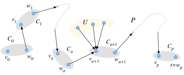
Figure 4. Illustration of the time analysis for arbitrary graphs.

Denote by $T$ the running time of protocol ArbGather. We have $T\leq\alpha_{\scriptscriptstyle\textrm{acy}}(C_{p})$ and $\alpha_{\scriptscriptstyle\textrm{scc}}(C_{0})=0$, so we can the express $T$ as

$$T\; =\;\sum_{a=0}^{p}\,[\,\alpha_{\scriptscriptstyle\textrm{acy}}(C_{a})-\alpha_{\scriptscriptstyle\textrm{scc}}(C_{a})\,]+\sum_{a=0}^{p-1}\,[\,\alpha_{\scriptscriptstyle\textrm{scc}}(C_{a+1})-\alpha_{\scriptscriptstyle\textrm{acy}}(C_{a})\,]\,.$$

We estimate the two terms separately. As explained earlier, we have $\alpha_{\scriptscriptstyle\textrm{acy}}(C_{a})=\alpha_{\scriptscriptstyle\textrm{scc}}(C_{a})+2\cdot T_{\scriptscriptstyle\textrm{SCC}}(C_{a})$, so the first term is at most

$$\sum_{a=0}^{p}\,[\,\alpha_{\scriptscriptstyle\textrm{acy}}(C_{a})-\alpha_{\scriptscriptstyle\textrm{scc}}(C_{a})\,]\; =\;2\cdot\sum_{a=0}^{p}T_{\scriptscriptstyle\textrm{SCC}}(C_{a})$$

$$=\;\sum_{a=0}^{p}{\tilde{O}}(n_{C_{a}}^{4/3})\;=\;{\tilde{O}}(n^{4/3}),$$

because $\sum_{a=0}^{p}n_{C_{a}}\leq n$. To estimate the second term, note that the definition of $v_{a+1}$ implies that $\alpha_{\scriptscriptstyle\textrm{scc}}(C_{a+1})=\alpha_{\scriptscriptstyle\textrm{scc}}(v_{a+1})$. Further, in the execution of AcyGather, node $w_{a}$ gets activated at time $\alpha_{\scriptscriptstyle\textrm{acy}}(C_{a})$. Then the analysis identical to that in Section 3 yields that we can estimate the second term by ${\tilde{O}}(n^{1.5})$.

As in the previous section, a more accurage bound follows by observing that in the analysis above we ignored three $\log n$ factors. We thus obtain the main result of this paper:

Theorem 4.1.

Let $G$ be an arbitrary digraph with $n$ vertices and a designated target node reachable from all other nodes. Algorithm ArbGather completes information gathering in $G$ in time $O(n^{1.5}\log^{3}n)$.

5. ${\tilde{O}}(n)$-Time Protocol With Acknowledgements for Acyclic Graphs

We now consider the problem of gathering in acyclic graphs with a weak form of acknowledgment of transmission success. To be more precise: Following each transmission from a node $v$, $v$ receives a single bit indicating whether at least one node successfully received that transmission ($v$ does not learn which specific node, or how many nodes in total, received the transmission). Our main goal in this section is to show that this single bit is enough to allow for gathering to be performed in time $O(n\log^{2}n)$ on acyclic graphs with $n$ vertices.The key idea here will be that nodes which have successfully transmitted can at least temporarily stop transmitting, making it easier for other nodes to succeed. In order for this to work, though, we need to guarantee that successful transmissions are occurring at a reasonable rate. The following combinatorial object will be our main tool for this.

We say that a collection $(S_{0},S_{1},\dots,S_{\ell-1})$ of label sets forms a $(n,k)$-half-selector if for every $X\subseteq[n]$ with $|X|\leq k$ there are at least $|X|/2$ choices of $x\in X$ for which there is an index $i$ with $S_{i}\cap X=\{x\}$ (in contrast to strong selectors where we want this property to hold for every choice of $x$). It is a consequence of Lemma 1 in [6] that for every $k$ there exists a half-selector of size $O(k\log n)$.

For all $j=0,1,\dots,\log n$, by ${\textsc{$2^{j}$-HalfSelect}}=(S_{0}^{j},S_{1}^{j},\dots,S_{b_{j}-1})$ we will denote a $2^{j}$-half-selector of size $b_{j}=O(2^{j}\log n)$. Without loss of generality we can also assume that $b_{j+1}=2b_{j}$ for all $i\leq\log n-1$, implying that $b_{j}=\gamma 2^{j}\log n$ for some absolute constant $\gamma$.

As in the previous sections, our algorithm will run on multiple frequencies, though this time the number of frequencies is $\kappa=\log n+2$. The intuition here is that for $0\leq j\leq\kappa-2$ frequency $j$ will be used to handle potential interferences involving at most $2^{j}$ vertices.

Protocol AcyGatherAck. At any given time step, a node can be either dormant or active. Initially the source nodes (with no in-neighbors) will be active and the remaining nodes will be dormant. Any active node transmits according to $2^{j}$-HalfSelect on each frequency $j=0,1,...,\kappa-2$, and according to RoundRobin on frequency $\kappa-1$. An active node which receives an acknowledgement of a successful transmission moves to the dormant state, and a dormant node which receives a transmission becomes active. Note that, unlike the previous algorithms, it is now possible for a node to become active multiple times during the process as it continually receives new rumors.

Correctness. As in the previous algorithms, correctness follows immediately from the inclusion of RoundRobin.

Running time. We claim that the running time of this protocol (with $\kappa$ frequencies) is $O(n\log n)$. Since $\kappa=O(\log n)$, this will give us an $O(n\log^{2}n)$-time protocol in the standard single-frequency model.

For a given node $v$, let ${\delta}(v)$ denote the length of the longest directed path from $v$ to the target node $t$. (This path cannot repeat vertices due to our assumption that $G$ is acyclic.) Let ${\delta^{\ast}}=\max_{v\in G}{\delta}(v)$. For $i=0,1,...,{\delta^{\ast}}$, let $B_{i}$ denote the set of nodes with ${\delta}(v)={\delta^{\ast}}-i$. (So $B_{\delta^{\ast}}={\left\{t\right\}}$ and $B_{0}$ consists of the nodes with the longest path to $t$). The following observation is immediate from the definition of $B_{i}$’s:

Observation 1.

If $i<i^{\prime}$ then there are no edges from $B_{i^{\prime}}$ to $B_{i}$. In particular, the vertices in $B_{0}$ have no incoming edges.

Let $\tau_{i}=4\gamma\sum_{p<i}|B_{i}|\log n$ for all $i$. (In particular, $\tau_{0}=0$.) Our running time bound would follow from the following claim:

Claim 3.

The following two properties hold for every $i=0,1,...,{\delta^{\ast}}$:

:

(i) All nodes in $\bigcup_{p<i}B_{p}$ remain dormant at all times after $\tau_{i}$ (inclusive).

:

(ii) At time $\tau_{i}$ each rumor is in $\bigcup_{p\geq i}B_{p}$.

In particular, at time $\tau_{{\delta^{\ast}}}=4\gamma\sum_{p=0}^{r-1}|B_{p}|\log n<4\gamma n\log n$ each rumor will be $t$.

We establish Claim 3 inductively. Both parts (i) and (ii) of the claim hold vacuously for $i=0$. Now suppose the claim is true for some $i$ and consider the computation of the nodes in $B_{i}$ beginning at time $\tau_{i}$. These nodes will not receive any rumors after time $\tau_{i}$ since, by the inductive hypothesis (i) and Observation 1, none of their in-neighbors will be active at any point. So any node in $B_{i}$ already dormant at time $\tau_{i}$ remains dormant, and any active node in it becomes permanently dormant once it succeeds at least once.

Choose $j$ such that $2^{j-1}<|B_{i}|\leq 2^{j}$. Let $A$ be the set of nodes in $B_{i}$ that are active at time $\tau_{i}$. Trivially, $|A|\leq|B_{i}|\leq 2^{j}$. Since the algorithm runs $2^{j}$-HalfSelect on frequency $j$, at least $|A|/2$ nodes in $A$ will have a time step in the interval $[\tau_{i},\tau_{i}+b_{j})$ when they will successfully transmit and become dormant. Thus, if $A^{\prime}$ is the set of nodes in $B_{i}$ that are active at time $\tau_{i}+b_{j}$, then $|A^{\prime}|\leq|A|/2\leq 2^{j-1}$. Next, we look at time interval $[\tau_{i}+b_{j},\tau_{i}+b_{j}+b_{j-1})$. Since the algorithm runs $2^{j-1}$-HalfSelect on frequency $j-1$, using the same argument, if $A^{\prime\prime}$ is the set of nodes in $B_{i}$ active at time $\tau_{i}+b_{j}+b_{j-1}$ then $|A^{\prime\prime}|\leq|A|/2\leq 2^{j-2}$. Continuing inductively, all the nodes in $A$ will succeed and become dormant no later than at time

$$\textstyle\tau_{i}+\sum_{q=0}^{j}b_{q}\; =\;\textstyle\tau_{i}+\gamma(\sum_{q=0}^{j}2^{q})\log n$$

$$<\;\tau_{i}+\gamma 2^{j+1}\log n$$

$$\leq\;\tau_{i}+4\gamma|B_{i}|\log n\textstyle\;=\;\tau_{i+1}.$$

Thus all the nodes in $B_{i}$ become dormant by time $\tau_{i+1}$ and will stay dormant, showing (ii). By Observation 1, each successful transmission from $B_{i}$ arrives at a node in $\sum_{p\geq i+1}B_{p}$, so part (ii) is also established. Concluding, we have proved the following theorem.

Theorem 5.1.

Let $G$ be an acyclic directed graph with $n$ vertices and a designated target node reachable from all other nodes. Using acknowledgements of successful transmissions, Algorithm AcyGatherAck completes information gathering in $G$ in time $O(n\log^{2}n)$.

6. Final Comments

In this paper we provided an ${\tilde{O}}(n^{1.5})$-time protocol for information gathering in ad-hoc radio networks, improving the trivial upper bound of $O(n^{2})$. For the model with transmissions acknowledgments we gave a ${\tilde{O}}(n)$-time protocol for acyclic graphs.

We hope that some ideas behind our algorithms will lead to further improvements, and perhaps find applications to other communication dissemination problems in ad-hoc radio networks. One idea that is particularly promising is the amortization technique in Section 3, where a failure of a node in transmitting its message is charged to stage indices of the interfering nodes. Another idea is the technique for integrating a gossiping protocol (applicable only to strongly connected digraphs) with an information gathering protocol for acyclic digraphs, to obtain an information gathering protocol for arbitrary digraphs. Using this technique, improving the upper bound to below ${\tilde{O}}(n^{1.5})$ should be possible by designing an appropriate protocol for the restricted case of acyclic graphs.

Several open problems remain. The two most intriguing problems are about the time complexity of gossiping and information gathering, as for both problems the best known lower bounds are only $\Omega(n\log n)$, the same as for broadcasting.

References

- [1] Noga Alon, Amotz Bar-Noy, Nathan Linial, and David Peleg. A lower bound for radio broadcast. J. Comput. Syst. Sci., 43(2):290–298, 1991.
- [2] Danilo Bruschi and Massimiliano Del Pinto. Lower bounds for the broadcast problem in mobile radio networks. Distributed Computing, 10(3):129–135, 1997.
- [3] Bogdan S. Chlebus, Leszek Gasieniec, Alan Gibbons, Andrzej Pelc, and Wojciech Rytter. Deterministic broadcasting in ad hoc radio networks. Distributed Computing, 15(1):27–38, 2002.
- [4] Marek Chrobak and Kevin P. Costello. Faster information gathering in ad-hoc radio tree networks. Algorithmica, 80(3):1013–1040, 2018.
- [5] Marek Chrobak, Kevin P. Costello, Leszek Gasieniec, and Dariusz R. Kowalski. Information gathering in ad-hoc radio networks with tree topology. Information and Computation, 258:1–27, 2018.
- [6] Marek Chrobak, Leszek Gasieniec, and Wojciech Rytter. Fast broadcasting and gossiping in radio networks. Journal of Algorithms, 43(2):177–189, 2002.
- [7] Marek Chrobak, Leszek Gasieniec, and Wojciech Rytter. A randomized algorithm for gossiping in radio networks. Networks, 43(2):119–124, 2004.
- [8] Andrea E. F. Clementi, Angelo Monti, and Riccardo Silvestri. Selective families, superimposed codes, and broadcasting on unknown radio networks. In Proc. 12th Annual Symposium on Discrete Algorithms (SODA’01), pages 709–718, 2001.
- [9] Andrea E. F. Clementi, Angelo Monti, and Riccardo Silvestri. Distributed broadcast in radio networks of unknown topology. Theor. Comput. Sci., 302(1-3):337–364, 2003.
- [10] Artur Czumaj and Peter Davies. Faster deterministic communication in radio networks. In 43rd International Colloquium on Automata, Languages, and Programming (ICALP’16), pages 139:1–139:14, 2016.
- [11] Artur Czumaj and Wojciech Rytter. Broadcasting algorithms in radio networks with unknown topology. Journal of Algorithms, 60(2):115 – 143, 2006.
- [12] Gianluca De Marco. Distributed broadcast in unknown radio networks. In 19th Annual ACM-SIAM Symposium on Discrete Algorithms (SODA’08), pages 208–217, 2008.
- [13] Antonio Fernández Anta, Miguel A. Mosteiro, and Jorge Ramón Muñoz. Unbounded contention resolution in multiple-access channels. Algorithmica, 67(3):295–314, 2013.
- [14] Leszek Gasieniec. On efficient gossiping in radio networks. In 16th Int. Colloquium on Structural Information and Communication Complexity (SIROCCO’09), pages 2–14, 2009.
- [15] Leszek Gasieniec. Deterministic broadcasting in radio networks. In Encyclopedia of Algorithms, pages 529–530. Springer US, 2016.
- [16] Leszek Gasieniec and Igor Potapov. Gossiping with unit messages in known radio networks. In Foundations of Information Technology in the Era of Networking and Mobile Computing, IFIP 17 World Computer Congress - TC1 Stream / 2 IFIP International Conference on Theoretical Computer Science (TCS’02), pages 193–205, 2002.
- [17] Leszek Gasieniec, Tomasz Radzik, and Qin Xin. Faster deterministic gossiping in directed ad hoc radio networks. In Scandinavian Workshop on Algorithm Theory (SWAT’04), pages 397–407, 2004.
- [18] Alon Itai. Randomized broadcasting in radio networks. In Encyclopedia of Algorithms, pages 1734–1738. 2016.
- [19] Tomasz Jurdzinski and Dariusz R. Kowalski. Wake-up problem in multi-hop radio networks. In Encyclopedia of Algorithms, pages 2352–2354. Springer, 2016.
- [20] Dariusz R. Kowalski and Andrzej Pelc. Faster deterministic broadcasting in ad hoc radio networks. SIAM J. Discrete Math., 18(2):332–346, 2004.
- [21] Eyal Kushilevitz and Yishay Mansour. An lower bound for broadcast in radio networks. SIAM J. Computg., 27(3):702–712, 1998.
- [22] Ding Liu and Manoj Prabhakaran. On randomized broadcasting and gossiping in radio networks. In 8th Annual Int. Conference on Computing and Combinatorics (COCOON’02), pages 340–349, 2002.
- [23] Gianluca De Marco and Dariusz R. Kowalski. Contention resolution in a non-synchronized multiple access channel. In Proc. of the 27th Int. Symposium on Parallel Distributed Processing (IPDPS), pages 525–533, 2013.
- [24] Gianluca De Marco and Dariusz R. Kowalski. Fast nonadaptive deterministic algorithm for conflict resolution in a dynamic multiple-access channel. SIAM Journal on Computing, 44(3):868–888, 2015.
- [25] David Peleg. Time-efficient broadcasting in radio networks: A review. In Distributed Computing and Internet Technology, 4th International Conference, ICDCIT 2007, Bangalore, India, December 17-20, Proceedings, pages 1–18, 2007.
- [26] Ying Xu. An deterministic gossiping algorithm for radio networks. Algorithmica, 36(1):93–96, 2003.