Curve Fitting from Probabilistic Emissions and Applications to Dynamic Item Response Theory

Abstract

Item response theory (IRT) models are widely used in psychometrics and educational measurement, being deployed in many high stakes tests such as the GRE aptitude test. IRT has largely focused on estimation of a single latent trait (e.g. ability) that remains static through the collection of item responses. However, in contemporary settings where item responses are being continuously collected, such as Massive Open Online Courses (MOOCs), interest will naturally be on the dynamics of ability, thus complicating usage of traditional IRT models. We propose DynAEsti, an augmentation of the traditional IRT Expectation Maximization algorithm that allows ability to be a continuously varying curve over time. In the process, we develop CurvFiFE, a novel non-parametric continuous-time technique that handles the curve-fitting/regression problem extended to address more general probabilistic emissions (as opposed to simply noisy data points). Furthermore, to accomplish this, we develop a novel technique called grafting, which can successfully approximate distributions represented by graphical models when other popular techniques like Loopy Belief Propogation (LBP) and Variational Inference (VI) fail. The performance of DynAEsti is evaluated through simulation, where we achieve results comparable to the optimal of what is observed in the static ability scenario. Finally, DynAEsti is applied to a longitudinal performance dataset (80-years of competitive golf at the 18-hole Masters Tournament) to demonstrate its ability to recover key properties of human performance and the heterogeneous characteristics of the different holes. Python code for CurvFiFE and DynAEsti is publicly available at github.com/chausies/DynAEstiAndCurvFiFE. This is the full version of our ICDM 2019 paper.

I Introduction

Traditional Item Response Theory (IRT) provides powerful tools for simultaneous analysis of both the latent traits of examinees and the characteristics of test items. As such, IRT models are quite popular. For example, many high stakes educational tests, such as the Graduate Record Examination (GRE), employ IRT. IRT is also deployed in other settings, such as healthcare, therapy, and quality-of-life research [1, 2]. In typical usage, the IRT framework conceptualizes ability as a static latent trait for each of the test takers. If item responses are collected over a drawn-out period of time (e.g., students over a 5-month semester), then ability should change dynamically across the window of observation. Indeed, this is the key goal of educational interventions. Students can work hard to raise their ability, or have their ability atrophy if they don’t keep studying. These fluctuations could be important feedback to pick up on. For example, a teacher may wish to reward improvement over time to encourage such behavior. As another example, one may wish to try various curricula to see which are effective at accelerating ability. Extending IRT models to cover such scenarios is a crucial psychometric need.

Over the years, initial work has been done to extend static IRT models to handle longitudinal and time series data [3, 4, 5]. Most recently, [6] proposes a treatment of this problem, Dynamic Item Response (DIR) models, based on Dynamic Linear Models (DLM), which are commonly used to model time series data. A crucial drawback of this approach (and the other previous approaches) is that these models for ability curves are highly parametric. In particular, they assume steady growth over time. While these are perhaps apt assumptions for specific use cases (e.g., growth in reading ability over time [6]), we have relatively limited understanding of many key dynamics of learning at this point. Thus, it seems optimal to, if possible, relax such parametric constraints. A more flexible approach could potentially allow us to uncover more complex and novel features of learning dynamics.

In this paper, we propose the DynAEsti algorithm. This is a non-parametric approach to generalizing static IRT that allows for dynamically changing ability curves for students, as opposed to a single static ability. The non-parametric nature of our approach allows us to capture a wider range of learning behaviors, such as how ability may atrophy in certain settings; we illustrate this point empirically later in the paper.

Central to the DynAEsti algorithm, we address the fundamental problem of generalizing the curve-fitting/regression problem to handle general probabilistic emissions (as opposed to only noisy data-points). A simple example demonstrating this problem is shown in Figure 1. John Smith is running for president of Mars, and we wish to estimate how he is polling in the 100 days leading up to the election. So each day, we ask a single random Mars citizen whether they will vote for Smith. Given these 100 uniformly spaced “emissions”, we wish to estimate the true curve representing what percentage of people will vote John Smith over time. Standard curve fitting techniques like spline smoothing cannot handle such general probabilistic emissions, and can only handle noisy data-points that were subject to symmetric Gaussian noise. In this paper, we propose CurvFiFE, our non-parametric continuous-time solution to this problem.

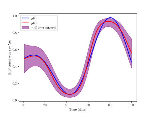
Figure 1: Performance of CurvFiFE demonstrated on a polling example. John Smith is running for president, and the percentage of people who will vote for him over time is estimated. $n=100$ people were polled uniformly spread over 100 days. $y(t)$ is the true percent of people who will vote for Smith. $\hat{y}(t)$ is the estimate of the curve from CurvFiFE. The shaded region shows the 70% (1 std) confidence interval for the marginal distribution on the estimated curve at each time.

Furthermore, as part of CurvFiFE, we develop grafting, a novel technique for approximating distributions represented as Graphical Models. Notably, this technique proves successful in this case where popular techniques like Loopy Belief Propogation (LBP) and Variational Inference (VI) fail.

The paper proceeds as follows. We offer a brief introduction to IRT in Section I-A. In Section II, we introduce the problem of dynamic ability estimation. In Section II-A, we detail the novel CurvFiFE algorithm, which provides the backbone for our solution to the problem. Then, in Section II-B, we detail DynAEsti, our solution to the dynamic ability estimation problem. In Section III, we examine the performance of the algorithm on simulated synthetic examples, where we achieve results comparable to the optimal of what is observed in the static scenario. In Section IV, we use DynAEsti to analyze a real-world dataset: 80 years of results for hundreds of golfers at the prestigious 18-hole Masters Tournament. Finally, in Section V, we make concluding remarks. Python code for CurvFiFE and DynAEsti is publicly available at github.com/chausies/DynAEstiAndCurvFiFE.

I-A Background on IRT

The prototypical setting for applications of IRT is one wherein $n$ students each respond to $m$ items. Students have static latent abilities $\Theta=\left[\theta_{1},\ldots,\theta_{n}\right]^{T}\in\mathbb{R}^{n}$, which affect their item responses. $R$ is the matrix of item responses, where $R_{ij}$ is the response of student $i$ to item $j$. For example, $R_{ij}=1$ could indicate a correct response from student $i$ to problem $j$. The item responses of a student are assumed to be independent conditioned on latent ability. Abilities are related to item responses via

$$\Pr[R_{ij}=r|\theta_{i}]=F(\theta_{i},\psi_{j},r)$$

where $F$ is the so-called Item Response Function (IRF), and $\psi_{j}$ is a vector of parameters associated with item $j$. For example, the popular 3-parameter logistic (3PL) IRF [7] for dichotomous responses $r\in\{0,1\}$ is given by

$$F(\theta,a,b,c,r)=\begin{cases}c+(1-c)\sigma\left(a(\theta-b)\right)&r=1\\ 1-F(\theta,a,b,c,1)&r=0\end{cases}$$

where

$$\sigma(z)=\frac{1}{1+\exp(-z)}$$

is the logistic function, and $\psi=(a,b,c)$ is the vector of item parameters. For some intuition, this IRF predicts that a student with higher ability is more likely to give a correct response. $b$ (the difficulty) is the “activation point”, which is around the ability needed to start giving correct responses with decently high probability. $a$ (the discrimination) indicates how sharp this transition is. $c$ (the guessing probability) gives how likely a student can give a correct response even with ability $\theta=-\infty$.

The entire system is identified by two sets of parameters: the abilities $\Theta$, and the item parameters $\Psi=\left[\psi_{1},\ldots,\psi_{m}\right]^{T}$. Given the $n\times m$ matrix of item responses $R$, the log-likelihood can be written as

$$\mathcal{L}(\Theta,\Psi)=\sum_{i,j}\log F(\theta_{i},\psi_{j},R_{ij}).$$

This log-likelihood can be efficiently and robustly optimized for a wide variety of IRFs using Expectation Maximization (EM). For details on this, see [8]. In a crude approximation, the EM consists of alternating between fixing one of $\Theta$ or $\Psi$, and optimizing $\mathcal{L}$ w.r.t. the other; a more precise statement involves alternating between an E-step and an M-step. In the E-step, one fixes $\Psi$ and then finds the distribution $p(\Theta)$ of $\Theta$. Then, in the M-step, one fixes the distribution $p(\Theta)$ and maximizes

$$\max_{\Psi}~{}\mathbb{E}_{p(\Theta)}\left(\mathcal{L}\left(\Theta,\Psi\right)\right)$$

to get an updated estimate for $\Psi$. Note that this expectation is taken over the (updated) distribution $p(\Theta)$. In practice, this leads to successful estimation of the problem parameters and the distributions on latent abilities for students simultaneously.

One appealing feature of this formulation is that the relevant calculations can be performed in parallel. It’s straightforward to split the log-likelihood into a sum of $n$ terms depending solely on their respective $\theta_{i}$. Or it can be split into a sum of $m$ terms depending solely on their respective $\psi_{j}$. So the E step can be broken into $n$ independent optimizations and the M step can be broken into $m$ independent optimizations. Within a step, these optimizations can be performed in parallel.

II Dynamic Ability Estimation

We formulate the Dynamic Ability Estimation problem as follows. There are $n$ students who respond to $m$ items. The students have latent ability curves $\Theta(t)=\left[\theta_{1}(t),\ldots,\theta_{n}(t)\right]^{T}$; that is, student $i$ has an ability of $\theta_{i}(t)$ at time $t$. At time $T_{ij}$, student $i$ responds to item $j$ to obtain a score of $R_{ij}$. The score a student gets on an item is dependent on only their ability at the time they respond to the item (e.g., scores are independent of prior abilities). That is to say,

$$\Pr\left[R_{ij}=r|\Theta,R_{(\tilde{i},\tilde{j})\neq(i,j)}\right] =\Pr[R_{ij}=r|\theta_{i}(T_{ij})]$$

$$=F(\theta_{i}(T_{ij}),\psi_{j},r)$$

where $F$ is some IRF with time-independent item parameters $\psi_{j}$.

To summarize, there are two data components of the dynamic ability estimation problem: $R$, the $n\times m$ matrix of item responses, and $T\in\mathbb{R}^{n\times m}$, the matrix of response times for each of the students to each of the items. There are also two sets of unobserved parameters. The abilities for each student over time are captured by $\Theta(t)$, and $\Psi=\left[\psi_{1},\ldots,\psi_{m}\right]^{T}$ contains the parameters for all of the items. The problem is to estimate $\Theta$ and $\Psi$ given $R$ and $T$. In the next two sections, we first detail the CurvFiFE algorithm, which is the backbone for our solution, enabling us to estimate $\theta_{i}$. We then detail our solution to the overall problem: DynAEsti.

II-A CurvFiFE

CurvFiFE (pronounced “covfefe”) is short for Curve Fitting From Emissions. It is a novel mathematical tool we developed to solve the general problem of fitting a curve when given “emissions”, which is a generalization of the regression problem. Normally, one is given many noisy data points, and tries to fit a smooth curve that’s “close” to them in some sense. This is a largely solved problem, with smoothing splines [9] being a standout solution. We focus on a challenging generalization. Instead of being given observations that are points on the curve plus noise, we instead observe “emissions”: values related to a point on the curve at a given time through a general conditional probability distribution.

More concretely, let us say there is a curve $y(t)$ which we wish to estimate. We observe triplets $(t_{i},e_{i},f_{i})$, $i\in\{1,\ldots,n\}$. These triplets identify the time $t_{i}$ at which an emission is observed as well as the emission $e_{i}$; the emission relates to $y\left(t_{i}\right)$, the curve’s value at the given time, through the emission distribution $f_{i}$,

$$f_{i}(y(t_{i}))=\Pr\left[\text{observing $e_{i}$ at time $t_{i}$}|y\left(t_{i}\right)\right].$$

From these emissions (and their distributions), we aim to estimate, or even find a distribution on, the curve $y$. That is, given any set of times $T=\left[\tau_{1},\ldots,\tau_{m}\right]^{T}$, one would like to estimate the joint distribution of $y(T)=\left[y(\tau_{1}),\ldots,y(\tau_{m})\right]^{T}$, the values of the curve at these times. This joint distribution on the curve at any set of times will be referred to as as the curve distribution $\mathcal{P}(y(T))$.

Returning to our polling example, Smith has a percentage of people who will vote for him $y(t)\in[0,1]$ that is changing over time. At different times $t_{i}$, a random person is polled by asking if they will vote for him, getting a response (i.e., an emission) $e_{i}\in\{\textit{Yes},\textit{No}\}$. In this simple case, the emission distribution is a Bernoulli with parameter $y(t_{i})$. In particular, assuming they said Yes, the corresponding emission distribution will be

$$f_{i}\left(y(t_{i})\right)=\textit{Bern}(y(t_{i});\textit{Yes})=y(t_{i})$$

If they said No, then the emission distribution would be

$$f_{i}\left(y(t_{i})\right)=\textit{Bern}(y(t_{i});\textit{No})=1-y(t_{i})$$

Traditional regression methods do not work here. For example, spline interpolation assumes that the noisy data points (which are indeed emissions) all come from symmetric Gaussian emission distributions, which is not necessarily always the case, as in the previous simple polling example where emissions were from non-symmetric Bernoulli distributions.

To solve this problem, we propose CurvFiFE. It is non-parametric, efficient (with its most costly operation being a constant number of matrix-multiplies), and has the very useful property that the resulting curve distribution $\mathcal{P}(y(T))$ it estimates is just a carefully chosen multivariate Gaussian distribution and thus easy to operate upon.

To summarize, given a set of emission triplets $(t_{1},e_{1},f_{1}),\ldots,(t_{n},e_{n},f_{n})$, CurvFiFE learns a curve distribution which will tell you

$$\mathcal{P}\left(y(T)\right)=\mathcal{N}(\mu,\Sigma;y(T))$$

where $\mu=\left[\mu_{1},\ldots,\mu_{m}\right]^{T}$ is the estimated means (e.g. $\mathbb{E}(y(\tau_{1}))=\mu_{1}$) and $\Sigma$ is the covariance matrix.

First, we assume that the range for the curve $y$ is $(-\infty,\infty)$, and that the marginal distribution of $y(t)$ is $\mathcal{N}(0,1)$ (the standard Gaussian) for all $t$. If this is not the case, then one need only apply a transform function $Q$ to the original curve so that it has the desired properties. For example, in the polling case where $y(t)$’s range is $[0,1]$ and perhaps had a Uniform prior, one could apply the probit transform $\Phi^{-1}(y(t))$ to get the curve to obey the assumed properties. After running CurvFiFE, one could apply the inverse transform $Q^{-1}$ to analyze the curve in its original space.

Broadly speaking, CurvFiFE finds the curve distribution through three steps:

1. Assume that all curves come from a reasonable prior distribution.

2. Given the prior distribution on the curve and some evidence (emissions), there is a theoretical (but intractable) form for the posterior distribution.

3. Approximate the posterior distribution as something tractable.

We emphasize that this approach is firmly rooted in probability theory, as opposed to relying on ad hoc heuristics. We will now detail and justify these steps.

In Step 1, the goal is to find a prior distribution on curves with the following properties:

1. Encodes properties of curves we would like to fit (e.g. they’re smooth),

2. Can capture a wide variety of behaviors (e.g. curves that increase, decrease, oscillate, etc.),

3. Is tractable and computationally convenient.

A flexible prior with these properties is the Gaussian Process prior [10]. Under this prior, the probability that a curve takes on values $y_{1},\ldots,y_{m}$ at times $\tau_{1},\ldots,\tau_{m}$ is distributed as a multivariate Gaussian $\mathcal{N}(0,\Sigma_{K})$, where the mean is $0$ and the covariance between any two points is

$$\llbracket\Sigma_{K}\rrbracket_{ij}=Cov(y_{i},y_{j})=K(|\tau_{i}-\tau_{j}|),$$

where $K(\Delta\tau)$ is known as the covariance function. For our purposes, it will be the Radial Basis Function (RBF)

$$K(\Delta\tau)=S^{2}\exp\left(-\frac{1}{2}\left(\frac{\Delta\tau}{h}\right)^{2}\right).$$ (1)

The intuition is that two temporally proximate points will have a correlation near 1 whereas points further apart will have weaker correlations. This powerful model for continuous-time regression also ensures that higher-order derivatives are smooth. We demonstrate the power of this model in Figure 2. The bandwidth $h$ controls how far apart in time two points must be before they start becoming less correlated; for a small $h$, curves can fluctuate rapidly in time. $S$ controls the magnitude of the curve’s fluctuations. For our purposes, we set $S=1$, since we assumed that points on the curve have a prior marginal distribution of $\mathcal{N}(0,1)$.

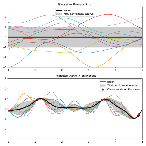
Figure 2: Demonstration of the Gaussian Process prior. In the first plot, sample curves from the prior are plotted, along with the average curve in bold black, and the 1 standard deviation confidence interval shaded in. In the second plot, the curve is fixed to go through the red points, yielding a posterior distribution on the curve. Again, samples, the mean, and the 1 std. confidence interval are plotted for this posterior distribution.

In Step 2, we consider evidence regarding the curve in the form of emissions, so we can consider the posterior distribution on the curve. Here, we make the note that, for now, we will only consider the curve points at the times of the emissions, $\left[y(t_{1}),\ldots,y(t_{n})\right]^{T}=\left[y_{1},\ldots,y_{n}\right]^{T}=Y$ (i.e., we do not consider $y(t)$ for $t$ at times where we do not observe emissions). The posterior distribution on these points, according to Bayes Rule, will be

$$p(Y|e_{1},\ldots,e_{n})\propto\mathcal{N}(0,\Sigma_{K};Y)\cdot\prod_{i=1}^{n}f_{i}(y_{i}).$$

In general, this is intractable to deal with. Even finding the posterior marginal distribution of a single $y_{i}$ is intractable. The one standout exception is if the emission distributions are Gaussian, because, in that case, you’re multiplying together a bunch of Gaussian factors, which will result in a Gaussian distribution that one could easily compute and do inference on.

In Step 3, we approximate the posterior distribution with a tractable alternative. We take a step back, and consider the problem as a Graphical Model; specifically a factor graph, which can be seen in Figure 3.

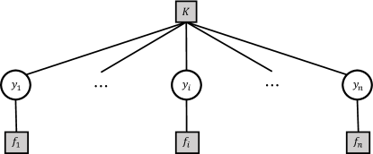
Figure 3: The factor graph corresponding to the curve $y$ at times $\tau_{1},\ldots,\tau_{n}$. Each circle represents a variable, and each square represents a factor. Note that the $K$ factor represents the Gaussian Process prior $\mathcal{N}(0,\Sigma_{K})$.

There are many established methods for trying to deal with factor graphs. However, all of these traditional methods and their variations completely fail for one reason or another. Just to address some of these:

1. Loopy Belief Propagation (LBP) is a popular method for estimating the posterior marginals for the variables [11]. It fails miserably in this case, however, because of the high degree of the $K$ factor, making LBP tantamount to manually marginalizing out the other $n-1$ variables.

2. Mean Field approximation (a type of Variational Inference [VI]) is a popular method for approximating an intractable distribution as a product of marginals [12]. However, it fails miserably in this case because the $K$ Gaussian factor is very nearly singular, with a large highest eigenvalue, and an extremely small lowest eigenvalue. The M-projection that VI finds mainly fits to this lowest eigenvalue, and so the approximation it finds is terrible.

3. LBP with the messages restricted to be Gaussian. This fails because, when one of the initial messages is $f_{i}$, it could be impossible to approximate such a message with a Gaussian. In particular, if $f_{i}(y_{i})=\frac{1}{1+\exp(-y_{i})}$ (a logistic emission distribution), that will stay at 1 as $y_{i}\to\infty$, which no Gaussian could capture.

Thus, in order to approximate this posterior distribution represented by a factor graph, we developed a novel technique which we dubbed grafting.

To motivate grafting, we return again to the polling example. There, the $f_{i}$’s were either $\textit{Bern}(y_{i};\textit{Yes})=y_{i}$ or else $\textit{Bern}(y_{i};\textit{No})=1-y_{i}$. Imagine that the points $y_{1},\ldots,y_{10}$ are very close together in time and so they were all essentially equal. This would mean that you could basically multiply all their factors together since they’re the same variable. Multiplying 10 of those factors together would give one bell-shaped factor that can be readily approximated as Gaussian. This gives the insight that, when many of the factors next to each other are combined, they’ll form a bell shape, which could have just as easily been formed by using some appropriate Gaussian factors instead. Grafting is a procedure by which we try to “cut off” the original factors $f_{i}$ and replace them with suitable Gaussian factors $g_{i}$ such that the overall distribution should look about the same whether one used the $f_{i}$ factor or the $g_{i}$ factor. In a sense, we’re “cutting off” the original factors, and “grafting on” Gaussian factors in their place (similar to grafting work with tree branches).

Each $g_{i}$ can be represented with a mean $m_{i}$ and a variance $v_{i}$. Let the vector of means and variances be $m$ and $v$ respectively. We find these $g_{i}$’s through an iterative improvement algorithm as follows. First, we initialize all the $g_{i}$’s to be standard Gaussians $\mathcal{N}(0,1)$. Then, in parallel, for each $g_{i}$, we do the following.

1. Assume every other $g_{j\neq i}$ has been perfectly chosen to replace every $f_{j\neq i}$; we set our focus on $g_{i}$.

2. We look at the marginal posterior distribution of $y_{i}$

   $$p(y_{i}) =\int p(Y)dy_{j\neq i}$$

   $$\propto f_{i}(y_{i})\cdot\int\left(\mathcal{N}(0,\Sigma_{K};Y)\cdot\prod_{j\neq i}f_{j}(y_{j})\right)dy_{j\neq i}$$

   $$\mathrel{\vbox{ \offinterlineskip\halign{\hfil$#$\cr\propto\cr\kern 2.0pt\cr\sim\cr\kern-2.0pt\cr}}}f_{i}(y_{i})\cdot\int\left(\mathcal{N}(0,\Sigma_{K};Y)\cdot\prod_{j\neq i}g_{j}(y_{j})\right)dy_{j\neq i}$$

   $$\propto f_{i}(y_{i})\cdot\mathcal{N}\left(\mu_{m},\sigma_{m}^{2};y_{i}\right)$$

   $$=p_{f}(y_{i})$$

   where $\mathcal{N}\left(\mu_{m},\sigma_{m}^{2}\right)$ can be called the “Gaussian message” from all the other variables to $y_{i}$. We compute this message.

3. We see that $p_{f}$ is just a product of two factors: a Gaussian message, and the original factor $f_{i}$. This product will be very nearly Gaussian. So we then choose $g_{i}$ such that

   $$p_{g}(y_{i})=g_{i}(y_{i})\cdot\mathcal{N}\left(\mu_{m},\sigma_{m}^{2};y_{i}\right)$$

   has the same mean and variance as $p_{f}(y_{i})$.

The previous steps update all the $g_{i}$’s in parallel. Then, one simply runs the previous steps over and over again until the $g_{i}$’s converge (in our experience, this takes roughly 15 iterations).

When the algorithm terminates, we’ve found Gaussian $g_{i}$’s that should serve as good replacements for the original $f_{i}$ factors. Thus, we have reduced the posterior to a Gaussian Process with Gaussian emission distributions. The posterior is now computationally tractable. What’s more, with Gaussian factors, we can also deal simply with the $y(\tau)$ for all the in-between times $\tau\neq t_{1},\ldots,t_{n}$.

Using this approach, given emission triplets $(t_{1},e_{1},f_{1}),\ldots,(t_{n},e_{n},f_{n})$, we can successfully approximate the true curve distribution via $\mathcal{P}(y(T))=\mathcal{N}(\mu,\Sigma;y(T))$. For implementation details, as well as the particulars of how to compute the $\mu_{m}$ and $\sigma_{m}^{2}$ for the Gaussian message, and how to compute $\mu$ and $\Sigma$ given $m$ and $v$, see the Appendix.

Finally, we make a few notes here related to the performance of this approach. First, the most costly operation in CurvFiFE is a constant number of matrix multiplies to find the Gaussian messages. So the runtime of the algorithm is $O(M(n))$, where $M(n)$ is the run-time of the matrix multiply algorithm used. Secondly, we note that the grafting procedure makes one major assumption which is that groups of emissions are close enough temporally that their factors can be combined to form a bell-shaped factor. This will usually be the case so long as one has been provided enough meaningful emissions. However, if it’s not the case, then grafting and CurvFiFE may fail. We also note that, in the case where emission distributions were in fact already Gaussian, then CurvFiFE converges in exactly 1 iteration.

The last note relates to the one hyperparameter in this method: the bandwidth $h$, which is the time-scale for the curve that decides how rapidly or slowly the curve is allowed to change. Unless one has expert input on what $h$ might be for the system, we recommend using $k$-fold Cross Validation (CV). Basically, to test an $h$, divide the emissions into $k$ sets, and for each set in turn, hold it out, run CurvFiFE using the other sets, and note the average log-likelihood assigned to the held-out emissions (with the averaging being done over the randomness in the curve distribution). Performance for $h$ is benchmarked using the average over the $k$ runs; a choice of $h$ is made by comparison of performance over small set of possible values for $h$.

In Figure 1, one can see the performance of CurvFiFE on a simulation of the polling example with $n=100$ uniformly placed emissions (with emissions being a random person getting polled).

II-B DynAEsti

In this section, we present our IRT-based extension, DynAEsti (pronounced “dynasty”), which is short for Dynamic Ability Estimation. As in traditional IRT, we estimate parameters using EM. When fixing the ability curves $\Theta$, estimating $\Psi$ is relatively similar to the standard case of static abilities; abilities at the corresponding times are used in place of a single static ability in updating of item parameters’ estimates. More concretely, the log-likelihood is

$$\mathcal{L}(\Psi|\Theta) =\sum_{i,j}\log F(\theta_{i}(T_{ij}),\psi_{j},R_{ij})$$

$$=\sum_{j}\left(\sum_{i}\log F(\theta_{i}(T_{ij}),\psi_{j},R_{ij})\right)$$

However, since we don’t have exact estimates for the curve $\theta_{ij}=\theta_{i}(T_{ij})$, we have to average over the distribution $p(\theta_{ij})$. And so the average likelihood function will be

$$\mathcal{L}(\Psi) =\sum_{j}\left(\sum_{i}\mathbb{E}_{p(\theta_{ij})}\left(\log F(\theta_{ij},\psi_{j},R_{ij})\right)\right).$$

Each of these terms can be computed efficiently for any particular $\Psi$. To maximize this w.r.t. $\Psi$, we use the L-BFGS-B algorithm, an efficient quasi-Newton optimization method [13].

On the other side, we have fixed $\Psi$ (and therefore, fixed IRFs), and the objective is to find smooth estimates for the ability curves $\Theta$. Recall that each of the curves can be dealt with independently. To estimate each of them, we use the CurvFiFE method described in Section II-A. We use the IRFs as the emission distributions, and for each ability curve $\theta_{i}$, we get the ability curve distribution $\mathcal{P}(\theta_{i}(T_{i}))$, as well as the marginal probability distributions $p(\theta_{i1}),\ldots,p(\theta_{im})$ needed for the M-step where we estimate the parameters.

This alternation between the two steps of estimating either $\Theta$ or $\Psi$ while leaving the other fixed (and using CurvFiFE as method for estimating curve distributions) is the DynAEsti algorithm. Like the vanilla IRT algorithm, this algorithm is also embarassingly parallel in exactly the same way. Computation involved in each of the individual steps is also efficient, using popular tools that have readily available implementations in popular programming languages. We implement Python code for CurvFiFE and DynAEsti, which is publicly available at github.com/chausies/DynAEstiAndCurvFiFE.

III Synthetic Example Performance

In this section, we apply DynAEsti to a synthetic dataset in order to demonstrate its performance.

III-A Construction of Dynamic Synthetic Data

For this example, we used $n=500$ students and $m=500$ items. The response times are uniformly spread from 0 to 1. That is to say, $T_{ij}=\frac{j-1}{m-1}$. A transformed 3PL IRF is used.

$$F(\theta,a,b,c,r)=$$

$$~{}~{}~{}\begin{cases}c+(1-c)\sigma\left(a\left(\Phi^{-1}(\theta)-\Phi^{-1}(b)\right)\right)&r=1\\ 1-F(\theta,a,b,c,1)&r=0\end{cases}$$

where $\Phi^{-1}$ is the quantile function for the standard normal distribution (a.k.a. the probit function), and $\sigma(z)=\frac{1}{1+\exp(-z)}$ is the logistic function. Normally, $\theta$ is assumed to have a standard normal distribution. With a probit-transform and the modified 3PL IRF, $\theta$ can be seen as coming from a uniform prior. This also makes it easier to demonstrate good estimation for the entire spectrum of abilities, since abilities are confined to the range $[0,1]$. Parameters for the IRFs are chosen randomly: $b$ is sampled from $\textit{Unif}[0,1]$, $c$ is sampled from $\textit{Unif}[0,0.2]$, and $a$ is sampled as $\exp(0.2\cdot Z)$, where $Z\sim\mathcal{N}(0,1)$.

We simulate ability curves as follows. First, a Latin Hypercube Sampling (as described in [14]) is done to get $n$ samples of the unit square $(\theta_{1}(0),\theta_{1}(1)),\ldots,(\theta_{n}(0),\theta_{n}(1))\in\left[0,1\right]^{2}$. This ensures an even sampling of starting and ending points for the ability curves. Then, given the beginning and ending points, the middle is filled out by sampling from a Gaussian Process with RBF covariance function 1 with $h=0.19$ and $S=0.6$. To learn more details about this procedure and Gaussian Process Regression, see [10]. Further note that, when necessary, the Gaussian Process was repeatedly sampled until the curve lay between 0 and 1.

This produces a wide range of highly varying ability curves. An example of what these curves might look like can be seen in Figure 4. These curves are perhaps more ill-behaved than we would expect in practice, but they serve as a “stress test”; our ability to recover such curves with fidelity would suggest that this method can handle even extremely complex learner dynamics alongside more straightforward cases.

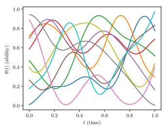
Figure 4: Example of the ability curves produced by the proposed Gaussian Process sampling procedure. For the sake of visualization, this figure demonstrates the curves produced when using only $n=10$.

Lastly, the matrix of scores $R$ is filled by sampling from the true IRFs conditioned on the true abilities at each time. With all that done, the DynAEsti procedure is run on the $R$ and $T$ matrices to produce estimates $\widehat{\Theta}$ and $\widehat{\Psi}$. DynAEsti is initialized with $\widehat{a}=1$, $\widehat{b}=0.5$, and $\widehat{c}=0$ as the starting guess for the parameters for each item.

Note that DynAEsti produces estimates of the distribution of each ability curve. But, for simplicity’s sake, we take the median ability curves to be our hard estimates and disregard the full distributions. That is to say, for all $t\in[0,1]$, we take $\widehat{\theta}_{i}(t)$ to be the median of the estimated marginal distribution on $\theta_{i}(t)$. The reason we take the median (as opposed to the mode or mean) is because, in preliminary testing, the median estimate performed very slightly better. Furthermore, the median is preserved by monotonic transformations (like the probit transform we use), which may be a desirable property.

III-B Parameter Recovery

A few examples are provided in Figure 5 to show how the estimates for the ability curves track the true ability curves. As can be seen, the estimates are reasonably accurate and err on the side of being smooth. This occurs because there is not enough data to reliably fit the higher-frequency undulations and the cross-validation scheme in CurvFiFE automatically understands this and errs on the side of smoothness.

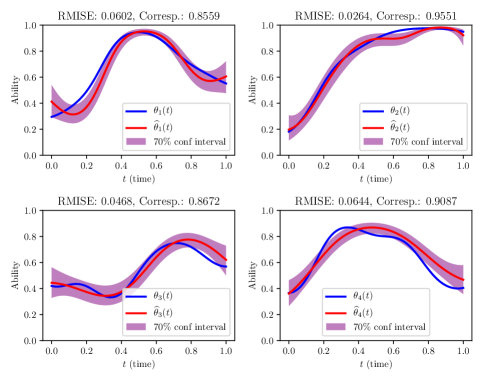
Figure 5: DynAEsti estimates (compared to truth) for 4 out of the 500 ability curves. The marginal 70% (1 std. div.) confidence interval for those estimates is also shown.

Here, we introduce some metrics in order to benchmark overall performance. Note that for a given IRF, several different triplets $(a,b,c)$ can correspond to similar looking IRFs [15], so $\left\|\psi-\widehat{\psi}\right\|$ isn’t a good measure of how far off the estimated IRF is from the true IRF. Instead, we use the Root Mean Integrated Squared Error (RMISE) between the true and estimated IRFs. The RMISE between a true function $f$ and its estimate $\widehat{f}$ is

$$RMISE(f,\widehat{f})=\sqrt{\int_{0}^{1}\left(f(x)-\widehat{f}(x)\right)^{2}dx}.$$

This gives a measure of the difference between the IRFs, with larger errors carrying heavier penalties.

As for the ability curves, it also makes sense to use the RMISE as a metric for quality of estimation. We also consider an additional metric as, in practice, one is mainly concerned with detecting fluctuations in the ability (i.e. When does ability dip? When does it surge?). For example, ascertaining whether learning is actually occurring and abilities aren’t remaining static could be a key objective. This motivates a metric which measures if changes in the true ability curve are reflected well by changes in the estimated ability curve. To capture this, we propose the correspondence metric (roughly speaking, the correlation between the derivatives of the true and estimated ability curves)

$$C(\theta,\widehat{\theta})=\frac{\int_{0}^{1}\theta^{\prime}(t)\cdot\widehat{\theta}^{\prime}(t)dt}{\sqrt{\int_{0}^{1}\left(\theta^{\prime}(t)\right)^{2}dt}\sqrt{\int_{0}^{1}\left(\widehat{\theta}^{\prime}(t)\right)^{2}dt}}\in[-1,1]$$

The correspondence between $\theta$ and $\widehat{\theta}$ is nothing but the cosine similarity between their derivatives, and ranges from 1 (full correspondence) to -1 (complete anti-correspondence).

To get a sense of what is optimal, we note here that, in the hypothetical perfectly static case (where abilities are completely static), we could use standard IRT. In this case, we would estimate the IRFs with an RMS RMISE of $0.039$ across all $m=500$ items, and we would estimate abilities with an RMS error of $0.047$ across all $n=500$ students. This gives a bound on what we could possibly achieve in the dynamic case. With these as benchmarks, we report the performance of DynAEsti in this simulated example. The IRFs were estimated with an RMS RMISE of $0.049$ across all items (compared to the optimal $0.039$). The ability curves were estimated with an RMS RMISE of $0.091$ across all students (compared to the optimal $0.047$). Furthermore, the average correspondence between the true and estimated ability curves is around $0.72$, with 80% having correspondence over $0.6$. In the cases where problems had lower correspondence, this was largely because the estimated curve was overly smooth while the true ability curve undulated rapidly; such undulations couldn’t be reliably captured due insufficient emissions.

IV Empirical Data Analysis: The Masters Golf Tournament

IV-A Background

Having developed DynAEsti, we demonstrate its utility by analysis of data from the Masters Golf Tournament. Considered by many to be the most prestigious golf tournament, the Masters has been going on since 1934 (over 80 years). It is the only major golf tournament to always take place at the exact same course: the famous Augusta National Golf Club. The course consists of 18 holes, and golfers try to complete each hole in as few strokes as possible. Each year, the Masters tournament sees around 100 golfers, who play the 18-hole course 4 times (rounds). Each hole has a pre-determined number of strokes that the golfers are expected to take for it; this is known as the hole’s “par”. Whoever has the fewest strokes over all 4 rounds at the end wins. Some players have attended over 35 of these tournaments. Tiger Woods, for example, has attended 21 of them.

While each stroke in golf is weighted equally in determining the tournament winner, this could be a suboptimal scheme for estimating ability (i.e., an unweighted sum over all strokes may be a worse predictor of future performance than an alternative estimation scheme). With that motivation, one may wish to identify the characteristics (e.g. the IRF) of each of the 18 holes, and how they reflect on underlying ability. However, standard IRT doesn’t allow for this. Each player’s ability may vary wildly over the decades they attend the tournament, so the assumption of a static ability would clearly be problematic. Furthermore, ability does not simply grow, but may also atrophy, as can be seen by comparing Tiger Woods’s record-breaking 1997 performance with some of his more recent performances. DynAEsti is designed to address these complicating factors so as to get high quality estimates for the IRFs of the holes, as well as the ability curves for the hundreds of golfers.

From the official Augusta Golf Club website, we have the scorecard for each player for each of their 4 rounds on the 18 holes for each of the years between 1937 and 2018 (barring years like those during WWII when the tournament wasn’t properly held).

The IRF we used to model the holes was a modified Generalized Partial Credit Model (GPCM) [16], which we call Golf IRF for convenience. For a particular hole, let

$$\omega_{s}(\theta)=\log\left(\frac{\Pr[\text{$s$ strokes below par}~{}|~{}\text{ability $\theta$}]}{\Pr[\text{par}~{}|~{}\text{ability $\theta$}]}\right)$$

be the log odds of getting $s$ strokes below par instead of a par given one has ability $\theta$. $s=1$ implies a “birdie” (one under par), and $s=-1$ implies a “bogey” (one over par). Clearly, $\omega_{0}(\theta)=0$. For each stroke count $s$ (besides $s=0$), there is an $a_{s}\in(0,\infty)$ (discrimination) parameter and a $b_{s}\in(-\infty,\infty)$ (difficulty) parameter. The log odds for $s$ is set to be

$$\omega_{s}(\theta)=sgn(s)\cdot\sum_{sgn(s)}^{s}a_{s}\cdot\left(\theta-b_{s}\right)$$

where $sgn(s)$ is the sign ($\pm 1$) of $s$. If $r=s-sgn(s)$ is the stroke one closer to par than $s$, then $b_{s}$ tells you the ability such that scoring an $s$ and scoring an $r$ are equally likely (their odds intersect). $a_{s}$ tells you how sharp the transition of odds between $r$ and $s$ is. Large $a_{s}$ means it’s a sharp transition from the odds being in favor of $r$ to being in favor of $s$. Small $a_{s}$ means a much flatter transition. To generate the probabilities of the stroke counts, we simply take a softmax of the log odds.

As a final note on the Golf IRF, we clipped (thresholded) the stroke counts to only allow for stroke counts that have had over 100 instances. For example, a triple bogey ($s=-3$) on hole #1 has only occurred 24 times in the history of the Masters. That’s far too few samples to reliably fit $a_{-3}$ and $b_{-3}$. Conversely, double bogeys ($s=-2$) have occurred 254 times, which is enough to fit. So all stroke counts $s<-2$ are just counted as double bogeys on hole #1.

IV-B Results

We use DynAEsti to estimate ability dynamics and features of the 18 holes at Augusta. In Figure 6, we can see the trajectories of the ability curves for the hundreds of golfers who’ve attended the Masters over the years. Figure 6 yields several insights. First, over the decades, abilities have generally increased. Given developments in golf-related technology and technique, this is quite reasonable. Second, for golfers who have participated in many Masters, there’s a common trend that ability initially grows, peaks, and then deteriorates (with perhaps a small “second wind” bump). This behavior is exemplified in Figure 7 by Jack Nicklaus and Arnold Palmer.

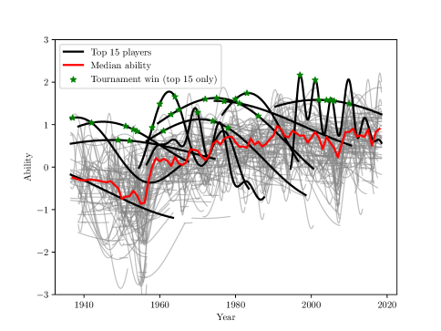
Figure 6: Ability curves over the years for the hundreds of Masters attendees. Those who only attended 1 Masters aren’t included. The highlighted top 15 golfers include Jack Nicklaus, Arnold Palmer, and Tiger Woods. The highest ability reached ever is Tiger Woods in 1997, during his record-breaking performance.

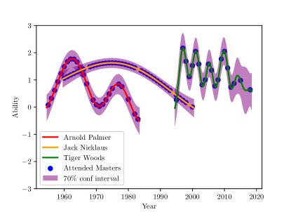
Figure 7: The ability curves for three legendary golfers, along with 70% (1 std. div.) confidence intervals on their abilities.

We now turn to the characteristics of the 18 holes. We note two main classes of interesting behavior here. On one hand, there are holes like hole #6, a.k.a. Juniper, whose IRF is in Figure 8. As can be seen, performance on the hole is fairly flat with respect to ability $\theta$. No matter where their ability lies between -2 and 2 (which is where most of the golfers are), a golfer makes par with $\approx 70\%$ chance, or gets unlucky and bogeys with $\approx 20\%$ chance. Changes in ability only change these odds slightly. This is due to the fact the hole has relatively low discrimination parameters $a$, and difficulty parameters $b$ that are too large in magnitude for typical abilities to compare to.

On the other hand, there are holes like #13, a.k.a. Azalea, whose IRF is in Figure 9. Performance on this hole is more strongly linked to ability. Consider the birdie ($s=1$) and par ($s=0$) curves. The ability needed to have a strong probability of obtaining a birdie is reasonable; moreover, the transition in odds is also fairly discriminative. Because it better allows golfers to demonstrate their ability, hole #13 discriminates golfers with respect to their ability more so than does hole #6.

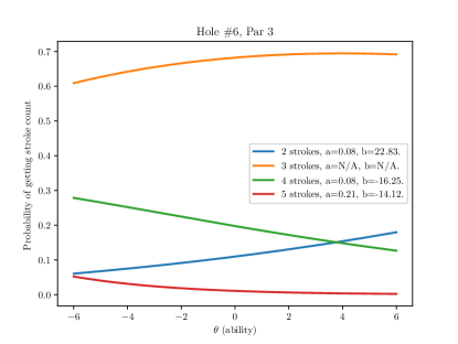
Figure 8: The IRF for the 6th hole of the masters, known as Juniper.

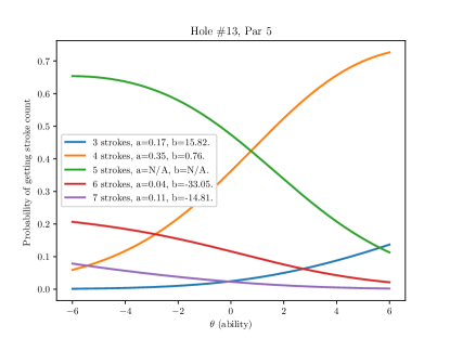
Figure 9: The IRF for the 13th hole of the masters, known as Azalea.

With this, it’s clear to see that not all strokes are created equal. For some holes, performance is mostly chance. On very few holes, performance is significantly affected by ability. Overall, a Masters tournament victory is not just about having high ability, but a lot about getting pretty lucky.

IV-C DynAEsti vs. Static IRT

As a final note, we demonstrate that DynAEsti’s allowance for dynamic ability curves is necessary to accurately model this golf example. Allowing for dynamic abilities yields far more accurate out-of-sample estimates than does traditional static IRT (SIRT). To motivate how we judge the schemes, consider that Arnold Palmer has participated in 25 different Masters, “responding” to (playing) 1800 holes in total. We compare performance by giving an algorithm (SIRT or DynAEsti) half of these responses to learn about Palmer’s ability, and then ask the scheme to assign a likelihood to the remaining half.

The particulars of how we judge are as follows.

1. Each scheme has to learn its own IRFs from scratch.

2. Averaged (geometrically) over 5 different runs:

   • Randomly divide Palmer’s 1800 responses into 2 halves.

   • Hold out 1 half, let the scheme learn Palmer’s ability using the other half, and then have the scheme assign a probability to observing the responses in the held-out half.

   • Switch the roles of the two halves, and take the geometric mean of the result.

Using this, we can get the (geometric) average probability that both DynAEsti and SIRT would assign to Palmer’s responses that it didn’t observe.

As one would imagine (see Figure 7), Palmer’s ability varied significantly over the decades he’s attended the Masters. SIRT does not account for this. For example, SIRT couldn’t use the fact that Palmer’s ability in the 1960’s was peak, and deteriorated in later years, whereas DynAEsti (via CurvFiFE) can pick up on that information. As a consequence, DynAEsti handily outperformed SIRT. On (geometric) average, DynAEsti assigned over 120 times higher likelihood to the held out responses than SIRT did.

V Conclusion and Further Research

IRT is a powerful framework for understanding item responses. In this paper, we proposed an extension of IRT, DynAEsti, that captures dynamically changing ability curves without relying on potentially unfounded parametric assumptions. We showed the performance of DynAEsti is comparable to a bound on the theoretically optimal performance. Furthermore, DynAEsti produces estimates of the ability curves with high correspondence to the true ability curves. As such, DynAEsti allows for high fidelity detection of ability growth and even potential decay. Thus, it may offer useful feedback for either the student or an administrator in digital learning environments (e.g., MOOCs) where item responses are being continuously collected.

DynAEsti allowed us to analyze the performance of golf players at the famous Masters tournament over the decades, where traditional static IRT would perform poorly. We were able to detect many interesting trends in player abilities over time as well as the characteristics of different holes. Finally, we showed how DynAEsti drastically outperforms static IRT in terms of its predictive power in this context.

To make this possible, we developed the CurvFiFE algorithm, which provided an efficient and non-parametric solution to the curve-fitting/regression problem extended to account for general probabilistic emissions. At the heart of this was the novel grafting technique we developed, which provided a means to approximate graphical models where standard LBP and VI techniques failed.

VI Appendix: CurvFiFE Implementation Details

Here, we will give some important implementation details for CurvFiFE that were left out of the main body of this paper.

The first note is that, we slightly modify the covariance function used to be

$$K(\Delta\tau)=K_{\text{RBF}}(\Delta\tau)+\epsilon\cdot\delta(\Delta\tau)$$

, where $\delta(\cdot)$ is the Dirac delta function, which is equal to 1 when its argument is 0, otherwise it is 0. This is essentially like adding a small amount onto the diagonal of the corresponding covariance matrix $\Sigma_{K}$.

The reason for this modification is to help with numerical stability, because $\Sigma_{K}$ is generally very nearly singular, with a high conditional number, so inverting it often yields numerical errors on finite-precision computers. We recommend $\epsilon=0.0001$.

Next, we give the formulae for the various calculations made by CurvFiFE. These formulae are presented without proof, but it just involves some simple matrix algebra, as well as the use of the Woodbury matrix identity, to derive them.

Given the previous guess for the Gaussian factors have means $m$ and variances $v$, the Gaussian messages with means $\eta=\left[\mu_{m}^{(1)},\ldots,\mu_{m}^{(n)}\right]^{T}$ and variances $\rho=\left[{\sigma_{m}^{(1)}}^{2},\ldots,{\sigma_{m}^{(n)}}^{2}\right]^{T}$ can be computed in parallel as follows.

$$P =\left(\Sigma_{K}^{-1}+Diag\left(\frac{1}{v}\right)\right)^{-1}$$

$$\widehat{\mu} =P\cdot\left(\frac{m}{v}\right)$$

$$H =P+\left(diag(P)\cdot\mathbf{1}_{n}^{T}\right)\circ P/\left((v-diag(P))\mathbf{1}_{n}^{T}\right)$$

$$M =\mathbf{1}_{n}\left(\frac{m}{v}\right)^{T}-Diag\left(\frac{m}{v}\right)$$

$$\rho =diag(H)$$

$$\eta =(H\circ M)\mathbf{1}_{n}$$

Note that division is element-wise, and $\circ$ is element-wise multiplication. Also, $\mathbf{1}_{n}$ is a length-$n$ column vector of ones.

Given the Gaussian messages, one computes the mean $\nu_{i}$ and variance $\gamma_{i}$ of each of the marginal $p_{f}(y_{i})$ distributions. This can be done in a straightforward manner by discretizing the $y_{i}$ number line (from say, -6 to 6), and computing the mean/variance from the discrete approximation to $p_{f}(y_{i})\propto f_{i}(y_{i})\cdot\mathcal{N}\left(\mu_{m}^{(i)},{\sigma_{m}^{(i)}}^{2};y_{i}\right)$.

Finally, given $\nu$ and $\gamma$, the following is how one computes the $m$ and $v$ for Gaussian factors in parallel.

$$v=\frac{1}{\frac{1}{\gamma}-\frac{1}{\rho}}$$

$$m=v\circ\left(\frac{\nu}{\gamma}-\frac{\eta}{\rho}\right)$$

The one thing of note here is that, sometimes, entries of $v$ may be negative, which occurs when an $f_{i}$ factor is particularly unsuited to a Gaussian approximation around the support of the $i$th Gaussian message. In this case, one essentially throws away that emission by replacing it with a Gaussian factor with infinite (or very large) variance $L$. In practice, we used $L=10^{6}$.

Lastly, having computed $m$ and $v$, we wish to find the distribution $\mathcal{N}(\mu,\Sigma)$ of $y(T)$ for any times $T=[\tau_{1},\ldots,\tau_{m}]^{T}$. This is done as follows.

$$\llbracket\Sigma_{1}\rrbracket_{ij} =\llbracket\Sigma_{K}\rrbracket_{ij}=K(|t_{i}-t_{j}|)$$

$$\llbracket\Sigma_{2}\rrbracket_{ij} =K(|\tau_{i}-\tau_{j}|)$$

$$\llbracket\Sigma_{12}\rrbracket_{ij} =K(|t_{i}-\tau_{j}|)$$

$$W =\Sigma_{12}^{T}\cdot\Sigma_{1}^{-1}\cdot\left(\Sigma_{1}^{-1}+Diag\left(\frac{1}{v}\right)\right)^{-1}$$

$$\Sigma =\Sigma_{2}+(W-\Sigma_{12}^{T})\cdot\Sigma_{1}^{-1}\cdot\Sigma_{12}$$

$$\mu =W\cdot\left(\frac{m}{v}\right)$$

As a final note, we implemented CurvFiFE and DynAEsti in Python 3, with all the main operations being done with the PyTorch library, assisted in part by Numpy and SciPy. This code for CurvFiFE and DynAEsti is publicly available at github.com/chausies/DynAEstiAndCurvFiFE.

References

- [1] B. B. Reeve, R. D. Hays, J. B. Bjorner, K. F. Cook, P. K. Crane, J. A. Teresi, D. Thissen, D. A. Revicki, D. J. Weiss, R. K. Hambleton, H. Liu, R. Gershon, S. P. Reise, J.-s. Lai, and D. Cella, “Psychometric evaluation and calibration of health-related quality of life item banks: plans for the patient-reported outcomes measurement information system (promis).,” Medical care, vol. 45, pp. S22–31, May 2007.
- [2] J. F. Fries, E. Krishnan, M. Rose, B. Lingala, and B. Bruce, “Improved responsiveness and reduced sample size requirements of promis physical function scales with item response theory,” Arthritis Research & Therapy, vol. 13, p. R147, Sep 2011.
- [3] N. D. Verhelst and C. A. W. Glas, “A dynamic generalization of the rasch model,” Psychometrika, vol. 58, pp. 395–415, Sep 1993.
- [4] P. C. M. Molenaar, “A dynamic factor model for the analysis of multivariate time series,” Psychometrika, vol. 50, pp. 181–202, Jun 1985.
- [5] T. Meiser, “Loglinear rasch models for the analysis of stability and change,” Psychometrika, vol. 61, pp. 629–645, Dec 1996.
- [6] X. Wang, J. O. Berger, and D. S. Burdick, “Bayesian analysis of dynamic item response models in educational testing,” The Annals of Applied Statistics, vol. 7, pp. 126–153, mar 2013.
- [7] A. L. Birnbaum, “Some latent trait models and their use in inferring an examinee’s ability,” Statistical theories of mental test scores, 1968.
- [8] Y. Hsu, “On the Bock-Aitkin procedure—From an EM algorithm perspective,” Psychometrika, vol. 65, pp. 547–549, Dec 2000.
- [9] C. H. Reinsch, “Smoothing by spline functions,” Numerische Mathematik, vol. 10, pp. 177–183, oct 1967.
- [10] C. E. Rasmussen, “Gaussian Processes in Machine Learning,” in Advanced Lectures on Machine Learning, pp. 63–71, Springer Berlin Heidelberg, 2004.
- [11] K. P. Murphy, Y. Weiss, and M. I. Jordan, “Loopy Belief Propagation for Approximate Inference: An Empirical Study,” in Proceedings of the Fifteenth Conference on Uncertainty in Artificial Intelligence, UAI’99, (San Francisco, CA, USA), pp. 467–475, Morgan Kaufmann Publishers Inc., 1999.
- [12] M. I. Jordan, Z. Ghahramani, T. S. Jaakkola, and L. K. Saul, “An Introduction to Variational Methods for Graphical Models,” Machine Learning, vol. 37, pp. 183–233, Nov 1999.
- [13] R. H. Byrd, P. Lu, J. Nocedal, and C. Zhu, “A Limited Memory Algorithm for Bound Constrained Optimization,” SIAM Journal on Scientific Computing, vol. 16, pp. 1190–1208, sep 1995.
- [14] K. Q. Ye, “Orthogonal Column Latin Hypercubes and Their Application in Computer Experiments,” Journal of the American Statistical Association, vol. 93, pp. 1430–1439, dec 1998.
- [15] G. Maris and T. Bechger, “On interpreting the model parameters for the three parameter logistic model,” Measurement Interdisciplinary Research and Perspectives, vol. 7, 05 2009.
- [16] G. N. Masters, “A rasch model for partial credit scoring,” Psychometrika, vol. 47, pp. 149–174, Jun 1982.