Neural Gaussian Copula for Variational Autoencoder

Abstract

Variational language models seek to estimate the posterior of latent variables with an approximated variational posterior. The model often assumes the variational posterior to be factorized even when the true posterior is not. The learned variational posterior under this assumption does not capture the dependency relationships over latent variables. We argue that this would cause a typical training problem called posterior collapse observed in all other variational language models. We propose Gaussian Copula Variational Autoencoder (VAE) to avert this problem. Copula is widely used to model correlation and dependencies of high-dimensional random variables, and therefore it is helpful to maintain the dependency relationships that are lost in VAE. The empirical results show that by modeling the correlation of latent variables explicitly using a neural parametric copula, we can avert this training difficulty while getting competitive results among all other VAE approaches.

1 Introduction

Variational Inference (VI) Wainwright et al. (2008); Hoffman et al. (2013) methods are inspired by calculus of variation Gelfand et al. (2000). It can be dated back to the 18th century when it was mainly used to study the problem of the change of functional, which is defined as the mapping from functions to real space and can be understood as the function of functions. VI takes a distribution as a functional and then studies the problem of matching this distribution to a target distribution using calculus of variation. After the rise of deep learning Krizhevsky et al. (2012), a deep generative model called Variational Autoencoder Kingma and Welling (2014); Hoffman et al. (2013) is proposed based on the theory of VI and achieves great success over a huge number of tasks, such as transfer learning Shen et al. (2017), unsupervised learning Jang et al. (2017), image generation Gregor et al. (2015), semi-supervised classification Jang et al. (2017), and dialogue generation Zhao et al. (2017). VAE is able to learn a continuous space of latent random variables which are useful for a lot of classification and generation tasks.

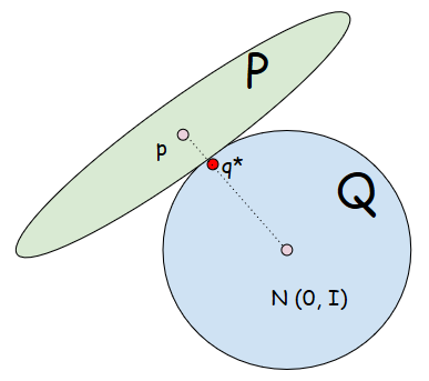
Figure 1: Intuitive illustration of VI: The elliptic $P$ is a distribution family containing the true posterior $p\in P$, and the circle $Q$ is a Mean-field variational family containing a standard normal prior $\mathcal{N}$. The optimal solution $q^{*}$ is the one in $Q$ that has the smallest $KL(q||p)$. In reality these two families may not overlap.

Recent studies Bowman et al. (2015); Yang et al. (2017); Xiao et al. (2018); Xu and Durrett (2018) show that when it comes to text generation and language modeling, VAE does not perform well and often generates random texts without making good use of the learned latent codes. This phenomenon is called Posterior Collapse, where the Kullback-Leibler (KL) divergence between the posterior and the prior (often assumed to be a standard Gaussian) vanishes. It makes the latent codes completely useless because any text input will be mapped to a standard Gaussian variable. Many recent studies Yang et al. (2017); Xu and Durrett (2018); Xiao et al. (2018); Miao et al. (2016); He et al. (2018) try to address this issue by providing new model architectures or by changing the objective functions. Our research lies in this second direction. We review the theory of VAE, and we argue that one of the most widely used assumptions in VAE, the Mean-field assumption, is problematic. It assumes that all approximated solutions in a family of variational distributions should be factorized or dimensional-wise independent for tractability. We argue that it leads to the posterior collapse problem since any variational posterior learned in this way does not maintain the correlation among latent codes and will never match the true posterior which is unlikely factorized.

We avert this problem by proposing a Neural Gaussian Copula (Copula-VAE) model to train VAE on text data. Copula Nelsen (2007) can model dependencies of high-dimensional random variables and is very successful in risk management Kole et al. (2007); McNeil et al. (2005), financial management Wang and Hua (2014), and other tasks that require the modeling of dependencies. We provide a reparameterization trick Kingma and Welling (2014) to incorporate it with VAE for language modeling. We argue that by maintaining the dependency relationships over latent codes, we can dramatically improve the performance of variational language modeling and avoid posterior collapse. Our major contributions can be summarized as the following:

• We propose Neural parameterized Gaussian Copula to get a better estimation of the posterior for latent codes.

• We provide a reparameterization technique for Gaussian Copula VAE. The experiments show that our method achieves competitive results among all other variational language modeling approaches.

• We perform a thorough analysis of the original VAE and copula VAE. The results and analysis reveal the salient drawbacks of VAE and explain how introducing a copula model could help avert the posterior collapse problem.

2 Related Work

Copula: Before the rise of Deep Learning

Copula Nelsen (2007) is a multivariate distribution whose marginals are all uniformly distributed. Over the years, it is widely used to extract correlation within high-dimensional random variables, and achieves great success in many subjects such as risk management Kole et al. (2007); McNeil et al. (2005), finance Wang and Hua (2014), civil engineeringChen et al. (2012); Zhang and Singh (2006), and visual description generation Wang and Wen (2015). In the past, copula is often estimated by Maximum Likelihood method Choroś et al. (2010); Jaworski et al. (2010) via parametric or semi-parametric approaches Tsukahara (2005); Choroś et al. (2010). One major difficulty when estimating the copula and extracting dependencies is the dimensionality of random variables. To overcome the curse of dimensionality, a graphical model called vine copula Joe and Kurowicka (2011); Czado (2010); Bedford et al. (2002) is proposed to estimate a high-dimensional copula density by breaking it into a set of bivariate conditional copula densities. However, this approach is often hand-designed which requires human experts to define the form of each bivariate copula, and hence often results in overfitting. Therefore, Gaussian copula Xue-Kun Song (2000); Frey et al. (2001) is often used since its multivariate expression has a simple form and hence does not suffer from the curse of dimensionality.

VAE for Text

Bowman et al. (2015) proposed to use VAE for text generation by using LSTM as encoder-decoder. The encoder maps the hidden states to a set of latent variables, which are further used to generate sentences. While achieving relatively low sample perplexity and being able to generate easy-to-read texts, the LSTM VAE often results in posterior collapse, where the learned latent codes become useless for text generation.

Recently, many studies are focusing on how to avert this training problem. They either propose a new model architecture or modify the VAE objective.  Yang et al. (2017) seeks to replace the LSTM Hochreiter and Schmidhuber (1997) decoder with a CNN decoder to control model expressiveness, as they suspect that the over-expressive LSTM is one reason that makes KL vanish.  Xiao et al. (2018) introduces a topic variable and pre-trains a Latent Dirichlet Allocation Blei et al. (2003) model to get a prior distribution over the topic information.  Xu and Durrett (2018) believes the bubble soup effect of high-dimensional Gaussian distribution is the main reason that causes KL vanishing, and therefore learns a hyper-spherical posterior over the latent codes.

3 Variational Inference

The problem of inference in probabilistic modeling is to estimate the posterior density $p(\mathbb{z}|\mathbb{x})$ of latent variable $\mathbb{z}$ given input samples $\{x_{i}\}_{i=1}^{D}$. The direct computation of the posterior is intractable in most cases since the normalizing constant $\int p(\mathbb{z},\mathbb{x})d\mathbb{z}$ lacks an analytic form. To get an approximation of the posterior, many approaches use sampling methods such as Markov chain Monte Carlo (MCMC) Gilks et al. (1995) and Gibbs sampling George and McCulloch (1993). The downside of sampling methods is that they are inefficient, and it is hard to tell how close the approximation is from the true posterior. The other popular inference approach, variational inference (VI) Wainwright et al. (2008); Hoffman et al. (2013), does not have this shortcoming as it provides a distance metric to measure the fitness of an approximated solution.

In VI, we assume a variational family of distributions $\mathcal{Q}$ to approximate the true posterior. The Kullback-Leibler (KL) divergence is used to measure how close $q\in Q$ is to the true $p(\mathbb{z}|\mathbb{x})$. The optimal variational posterior $q*\in Q$ is then the one that minimizes the KL divergence

$$KL(q||p)=\sum q(\mathbb{z}|\mathbb{x})log\frac{q(\mathbb{z}|\mathbb{x})}{p(\mathbb{z}|\mathbb{x})}$$

Based on this, variational autoencoder (VAE) Kingma and Welling (2014) is proposed as a latent generative model that seeks to learn a posterior of the latent codes by minimizing the KL divergence between the true joint density $p_{\theta}(\mathbb{x},\mathbb{z})$ the variational joint density $q_{\phi}(\mathbb{z},\mathbb{x})$. This is equivalent to maximizing the following evidence lower bound ELBO,

$$\mathcal{L}(\mathbb{\theta};\mathbb{\phi};\mathbb{x}) =-KL(q_{\phi}(\mathbb{z},\mathbb{x})||p_{\theta}(\mathbb{x},\mathbb{z}))$$

$$=\operatorname{\mathbb{E}}_{q(\mathbb{x})}[\operatorname{\mathbb{E}}_{q_{\phi}(\mathbb{z}|\mathbb{x})}[\log p_{\theta}(\mathbb{x}|\mathbb{z})]$$

$$\qquad-KL(q_{\phi}(\mathbb{z}|\mathbb{x})||p(\mathbb{z}))]$$

In this case, Mean-field Kingma and Welling (2014) assumption is often used for simplicity. That is, we assume that the members of variational family $Q$ are dimensional-wise independent, meaning that the posterior $q$ can be written as $q(\mathbb{z}|\mathbb{x})=\prod_{i=1}^{D}q(z_{i}|\mathbb{x})$. The simplicity of this form makes the estimation of ELBO very easy. However, it also leads to a particular training difficulty called posterior collapse, where the KL divergence term becomes zero and the factorized variational posterior collapses to the prior. The latent codes $\mathbb{z}$ would then become useless since the generative model $p(\mathbb{x}|\mathbb{z})$ no longer depends on it.

We believe the problem comes from the nature of variational family itself and hence we propose our Copula-VAE which makes use of the dependency modeling ability of copula model to guide the variational posterior to match the true posterior. We will provide more details in the following sections.

We hypothesize that the Mean-field assumption is problematic itself as the $q$ under this assumption can never recover the true structure of $p$. On the other hand, Copula-VAE makes use of the dependency relationships maintained by a copula model to guide the variational posterior to match the true posterior. Our approach differs from Copula-VI Tran et al. (2015) and Gaussian Copula-VAE Suh and Choi (2016) in that we use copula to estimate the joint density $p(\mathbb{z})$ rather than the empirical data density $p(\mathbb{x})$.

4 Our Approach: Neural Gaussian Copula

4.1 Gaussian Copula

In this section, we review the basic concepts of Gaussian copula. Copula is defined as a probability distribution over a high-dimensional unit cube $[0,1]^{d}$ whose univariate marginal distributions are uniform on $[0,1]$. Formally, given a set of uniformaly distributed random variables $U_{1},U_{2},...,U_{n}$, a copula is a joint distribution defined as

$$C(u_{1},u_{2},...,u_{n})=P(U_{1}\leq u_{1},...,U_{n}\leq u_{n})$$

What makes a copula model above so useful is the famous Sklar’s Theorem. It states that for any joint cumulative distribution function (CDF) with a set of random variables $\{x_{i}\}_{1}^{d}$ and marginal CDF $F_{i}(x_{i})=P(X_{i}\leq x)$, there exists one unique copula function such that the joint CDF is

$$F(x_{1},...,x_{d})=C(F_{1}(x_{1}),...,F_{d}(x_{d}))$$

By probability integral transform, each marginal CDF is a uniform random variable on $[0,1]$. Hence, the above copula is a valid one. Since for each joint CDF, there is one unique copula function associated with it given a set of marginals, we can easily construct any joint distribution whose marginal univariate distributions are the ones $F_{i}(x_{i})$ that are given. And, for a given joint distribution, we can also find the corresponding copula which is the CDF function of the given marginals.

A useful representation we can get by Sklar’s Theorem for a continuous copula is,

$$C(u_{1},...u_{d}) =F(F_{1}^{-}(u_{1}),...,F_{d}^{-}(u_{d}))$$

If we further restrict the marginals to be Gaussian, then we can get an expression for Gaussian copula, that is,

$$C_{\Sigma}(u_{1},...,u_{d})=\Phi(\Phi_{1}^{-}(u_{1}),...,\Phi_{d}^{-}(u_{d});0,\Sigma)$$

where $\Phi(\cdot;\Sigma)$ is the CDF of a multivariate Gaussian Distribution $\mathcal{N}(0,\Sigma)$, and $\{\Phi_{i}^{-}\}$ is the inverse of a set of marginal Gaussian CDF.

To calculate the joint density of a copula function, we take the derivative with respect to random variables $u$ and get

$$c_{\Sigma}(u_{1},...,u_{d}) =\frac{\partial C_{\Sigma}(u_{1},...,u_{d})}{\partial u_{1}\cdots u_{d}}$$

$$=\frac{\partial C_{\Sigma}(u_{1},...,u_{d})}{\partial q_{1}\cdots q_{d}}\prod^{d}_{i=1}\frac{\partial q_{i}}{\partial u_{i}}$$

$$=(\prod_{i=1}^{d}\sigma_{i})|\Sigma^{-1/2}|exp(-\frac{1}{2}q^{T}Mq)$$

where $M=\Sigma^{-}-diag(\Sigma)^{-}$, and $q_{i}=\Phi_{i}^{-}(u_{i})$.

Then, if the joint density $p(x_{1},...,x_{d})$ has a Gaussian form, it can be expressed by a copula density and its marginal densities, that is,

$$p(x_{1},...,x_{d}) =\frac{\partial F(\cdot)}{\partial x_{1}\cdots x_{d}}$$

$$=\frac{\partial C_{\Sigma}(\cdot)}{\partial u_{1}\cdots u_{d}}\prod\frac{\partial u_{i}}{\partial x_{i}}$$

$$=c_{\Sigma}(u_{1},...,u_{d})\prod_{i}p(x_{i})$$

Therefore, we can decompose the problem of estimating the joint density into two smaller sub-problems: one is the estimation for the marginals; the other is the estimation for the copula density function $c_{\Sigma}$. In many cases, we assume independence over random variables due to the intractability of the joint density. For example, in the case of variational inference, we apply Mean-Field assumption which requires the variational distribution family to have factorized form so that we can get a closed-form KL divergence with respect to the prior. This assumption, however, sacrifices the useful dependency relationships over the latent random variables and often leads to training difficulties such as the posterior collapse problem. If we assume the joint posterior of latent variables to be Gaussian, then the above Gaussian copula model can be used to recover the correlation among latent variables which helps obtain a better estimation of the joint posterior density. In the VAE setting, we can already model the marginal independent posterior of latent variables, so the only problem left is how to efficiently estimate the copula density function $c_{\Sigma}$. In the next section, we introduce a neural parameterized Gaussian copula model, and we provide a way to incorporate it with the reparameterization technique used in VAE.

4.2 Neural Gaussian Copula for VI

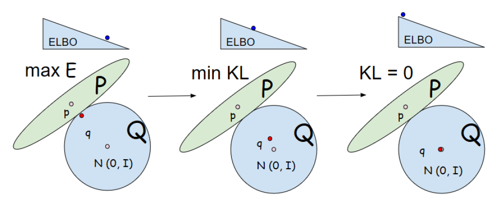
Figure 2: Training stage of VAE. Initially, the model tries to maximize ELBO by maximizing $\operatorname{\mathbb{E}}_{q(\mathbb{z}|\mathbb{x})}[p(\mathbb{x}|\mathbb{z})]$. Once $\operatorname{\mathbb{E}}_{q(\mathbb{z}|\mathbb{x})}[p(\mathbb{x}|\mathbb{z})]$ is maximized, the model maximizes ELBO by minimizing KL. During this stage, the posterior starts to move closer to the prior. In the final stage, the posterior collapses to the prior. But, the ELBO and $\operatorname{\mathbb{E}}_{q(\mathbb{z}|\mathbb{x})}[p(\mathbb{x}|\mathbb{z})]$ are already maximized, which means the model keeps constraining KL and there are not enough gradients to move the posterior away from the prior anymore.

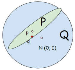
Figure 3: Ideal final stage of Copula-VAE. The family of distributions that contains the true posterior is now a subset of the variational family.

By Mean-field assumption, we construct a variational family $\mathcal{Q}$ assuming that each member $q\in\mathcal{Q}$ can be factorized,

$$q(\mathbb{z})=\prod_{i}^{d}q(z_{i})$$

This assumption, however, loses dependencies over latent codes and hence does not consider the non-factorized form of the true posterior. In this case, as pictured by Figure 2, when we search the optimal $q$*, it will never reach to the true posterior $p$. If we relieve the assumption, the variational family may overlap with the posterior family. However, this is intractable as the Monto Carlo estimator with respect to the objective often has very high variance Kingma and Welling (2014). Hence, we need to find a way to make it possible to match the variational posterior with the true posterior while having a simple and tractable objective function so that the gradient estimator of the expectation is simple and precise.

This is where Gaussian Copula comes into the story. Given a factorized posterior, we can construct a Gaussian copula for the joint posterior,

$$q_{\phi}(\mathbb{z}|x)=c_{\Sigma}(\Phi_{1}(z_{1}),...\Phi(z_{d}))\prod_{i}^{d}q_{\phi}(z_{i}|x)$$

where $c_{\Sigma}$ is the Gaussian copula density. If we take the log on both sides, then we have,

$$\log q_{\phi}(\mathbb{z}|x)=\log c_{\Sigma}(u_{1},...,u_{d})+\sum_{i}^{d}\log q_{\phi}(z_{i}|x)$$

Note that the second term on the right hand side is just the factorized log posterior we have in the original VAE model. By reparameterization trick Kingma and Welling (2014), latent codes sampled from the posterior are parameterized as a deterministic function of $\mu$ and $\sigma^{2}$, that is, $\mathbb{z}=\mu+\sigma\cdot\epsilon$, $\epsilon\sim\mathcal{N}(0,I)$, where $\mu,\sigma^{2}$ are parameterized by two neural networks whose inputs are the final hidden states of the LSTM encoder. Since $\prod_{i}q_{\phi}(z_{i}|x)=\mathcal{N}(\mu,\sigma^{2}I)$, we can compute the sum of log density of posterior by,

$$\sum_{i}^{d}\log q_{\phi}(z_{i}|x) =-\sum_{i}^{d}\log|\sigma_{i}|-\sum_{i}^{d}\frac{(z_{i}-\mu_{i})^{2}}{2\sigma_{i}^{2}}$$

$$-\frac{d}{2}\log 2\pi$$

Now, to estimate the log copula density $\log c_{\Sigma}(\cdot)$, we provide a reparameterization method for the copula samples $q\sim C_{\Sigma}(\Phi_{1}(q_{1}),...\Phi(q_{d}))$. As suggested by  Kingma and Welling (2014); Hoffman et al. (2013), reparameterization is needed as it gives a differentiable, low-variance estimator of the objective function. Here, we parameterize the copula samples with a deterministic function with respect to the Cholesky factor $L$ of its covariance matrix $\Sigma$. We use the fact that for any multivariate Gaussian random variables, a linear transformation of them is also a multivariate Gaussian random variable. Formally, if $X\sim\mathcal{N}(\mu,\Sigma)$, and $Y=AX$, then we must have $Y\sim\mathcal{N}(A\mu,A\Sigma A^{T})$. Hence, for a Gaussian copula with the form $c_{\Sigma}=\mathcal{N}(0,\Sigma)$, we can reparameterize its samples $q$ by,

$$\epsilon \sim\mathcal{N}(0,I)$$

$$q =L\cdot\epsilon$$

It is easy to see that $q=L\cdot\epsilon\sim\mathcal{N}(0,LI^{-}L^{T}=\Sigma)$ is indeed a sample from the Gaussian copula model. This is the standard way of sampling from Gaussian distribution with covariance matrix $LL^{T}$. To ensure numerical stability of the above reparameterization and to ensure that the covariance $\Sigma=LL^{T}$ is positive definite, we provide the following algorithm to parameterize $L$.

  h = LSTM(x)

  $w$ = ReLU($W_{1}\cdot h+b_{1}$)

  $a$ = Tanh($W_{2}\cdot h+b_{2}$)

  $\Sigma$ = $w\cdot I+aa^{T}$

  L = CholeskyFactorization($\Sigma$)

Algorithm 1 Neural reparameterization of Copula: Cholesky approach

the company said it will be sold to the company ’s promotional programs and _UNK

the company also said it will sell $ n million of soap eggs turning millions of dollars

the company said it will be _UNK by the company ’s _UNK division n

the company said it would n’t comment on the suit and its reorganization plan

mr . _UNK said the company ’s _UNK group is considering a _UNK standstill agreement with the company

traders said that the stock market plunge is a _UNK of the market ’s rebound in the dow jones industrial average

one trader of _UNK said the market is skeptical that the market is n’t _UNK by the end of the session

the company said it expects to be fully operational by the company ’s latest recapitalization

i was excited to try this place out for the first time and i was disappointed .

the food was good and the food a few weeks ago , i was in the mood for a _UNK of the _UNK

i love this place . i ’ ve been here a few times and i ’ m not sure why i ’ ve been

this place is really good . i ’ ve been to the other location many times and it ’s very good .

i had a great time here . i was n’t sure what i was expecting . i had the _UNK and the

i have been here a few times and have been here several times . the food is good , but the food is good

this place is a great place to go for lunch . i had the chicken and waffles . i had the chicken and the _UNK

i really like this place . i love the atmosphere and the food is great . the food is always good .

Table 1: Qualitative comparison between VAE and our proposed approach. First row: PTB samples generated from prior $p(\mathbb{z})$ by VAE (upper half) and copula-VAE (lower half). Second row: Yelp samples generated from prior $p(\mathbb{z})$ by VAE (upper half) and copula-VAE (lower half).

In Algorithm 1, we first parameterize the covariance matrix and then perform a Cholesky factorization Chen et al. (2008) to get the Cholesky factor $L$. The covariance matrix $\Sigma=w\cdot I+aa^{T}$ formed in this way is guaranteed to be positive definite. It is worth noting that we do not sample the latent codes from Gaussian copula. In fact, $\mathbb{z}$ still comes from the independent Gaussian distribution. Rather, we get sample $q$ from Gaussian copula $C_{\Sigma}$ so that we can compute the log copula density term in the following, which will then be used as a regularization term during training, in order to force the learned $\mathbb{z}$ to respect the dependencies among individual dimensions.

Now, to calculate the log copula density, we only need to do,

$$\log c_{\Sigma} =\sum_{i}^{d}\log\sigma_{i}-1/2\log|\Sigma|+1/2q^{T}Mq$$

where $M=diag(\Sigma^{-})-\Sigma^{-}$.

To make sure that our model maintains the dependency structure of the latent codes, we seek to maximize both the ELBO and the joint log posterior likelihood $\log q(\mathbb{z}|\mathbb{x})$ during the training. In other words, we maximize the following modified ELBO,

$$\mathcal{L^{\prime}}=\mathcal{L}+\lambda(\log c_{\Sigma}(\cdot)+\sum_{i}^{d}\log q_{\phi}(z_{i}|\mathbb{x}))$$

where $\mathcal{L}$ is the original ELBO. $\lambda$ is the weight of log density of the joint posterior. It controls how good the model is at maintaining the dependency relationships of latent codes. The reparameterization tricks both for $\mathbb{z}$ and $q$ makes the above objective fully differentiable with respect to $\mu,\sigma^{2},\Sigma$. Maximizing $\mathcal{L^{\prime}}$ will then maximize the log input likelihood $\log p(\mathbb{x})$ and the joint posterior log-likelihood $\log q(\mathbb{z}|\mathbb{x})$. If the posterior collapses to the prior and has a factorized form, then the joint posterior likelihood will not be maximized since the joint posterior is unlikely factorized. Therefore, maximizing the joint posterior log-likelihood along with ELBO forces the model to generate readable texts while also considering the dependency structure of the true posterior distribution, which is never factorized.

4.3 Evidence Lower Bound

Another interpretation can be seen by taking a look at the prior. If we compose the copula density with the prior, then, like the non-factorized posterior, we can get the non-factorized prior,

$$\log p_{\theta}(\mathbb{z})=\log c_{\Sigma}(u_{1},...,u_{d})+\sum_{i}^{d}\log p_{\theta}(z_{i})$$

And the corresponding ELBO is,

$$\mathcal{L}(\mathbb{\theta};\mathbb{\phi};\mathbb{x}) =\operatorname{\mathbb{E}}_{q(\mathbb{x})}[\operatorname{\mathbb{E}}_{q_{\phi}(\mathbb{z}|\mathbb{x})}[\log p_{\theta}(\mathbb{x}|\mathbb{z})]$$

$$\qquad-KL(q_{\phi}(\mathbb{z}|\mathbb{x})||p_{\theta}(\mathbb{z}))]$$

$$=\operatorname{\mathbb{E}}_{q(\mathbb{x})}[\operatorname{\mathbb{E}}_{q_{\phi}(\mathbb{z}|\mathbb{x})}[\log p_{\theta}(\mathbb{x}|\mathbb{z})]$$

$$\qquad-\operatorname{\mathbb{E}}_{q_{\phi}(\mathbb{z}|\mathbb{x})}[\log q_{\phi}(\mathbb{z}|\mathbb{x})-\log p(\mathbb{z})]$$

$$\qquad\qquad+\operatorname{\mathbb{E}}_{q_{\phi}(\mathbb{z}|\mathbb{x})}[\log c_{\Sigma}(u_{1},...,u_{d})]]$$

Like Normalizing flow Rezende and Mohamed (2015), maximizing the log copula density will then learns a more flexible prior other than a standard Gaussian. The dependency among each $z_{i}$ is then restored since the KL term will push the posterior to this more complex prior.

We argue that relieving the Mean-field assumption by maintaining the dependency structure can avert the posterior collapse problem. As shown in Figure 2, during the training stage of original VAE, if kl-annealing Bowman et al. (2015) is used, the model first seeks to maximize the expectation $\operatorname{\mathbb{E}}_{q(\mathbb{z}|\mathbb{x})}[p(\mathbb{x}|\mathbb{z})]$. Then, since $q(\mathbb{z}|\mathbb{x})$ can never reach to the true $p(\mathbb{z}|\mathbb{x})$, $q$ will reach to a boundary and then the expectation can no longer increase. During this stage, the model starts to maximize the ELBO by minimizing the KL divergence. Since the expectation is maximized and can no longer leverage KL, the posterior will collapse to the prior and there is not sufficient gradient to move it away since ELBO is already maximized. On the other hand, if we introduce a copula model to help maintain the dependency structure of the true posterior by maximizing the joint posterior likelihood, then, in the ideal case, the variational family can approximate distributions of any forms since it is now not restricted to be factorized, and therefore it is more likely for $q$ in Figure 3 to be closer to the true posterior $p$. In this case, the $\operatorname{\mathbb{E}}_{q(\mathbb{z}|\mathbb{x})}[p(\mathbb{x}|\mathbb{z})]$ can be higher since now we have latent codes sampled from a more accurate posterior, and then this expectation will be able to leverage the decrease of KL even in the final training stage.

5 Experimental Results

5.1 Datasets

Data	Train	Valid	Test	Vocab
Yelp13	62522	7773	8671	15K
PTB	42068	3370	3761	10K
Yahoo	100K	10K	10K	20K

Table 2: Size and vocabulary size for each dataset.

In the paper, we use Penn Tree Marcus et al. (1993), Yahoo Answers Xu and Durrett (2018); Yang et al. (2017), and Yelp 13 reviews Xu et al. (2016) to test our model performance over variational language modeling tasks. We use these three large datasets as they are widely used in all other variational language modeling approaches Bowman et al. (2015); Yang et al. (2017); Xu and Durrett (2018); Xiao et al. (2018); He et al. (2018); Kim et al. (2018). Table 2 shows the statistics, vocabulary size, and number of samples in Train/Validation/Test for each dataset.

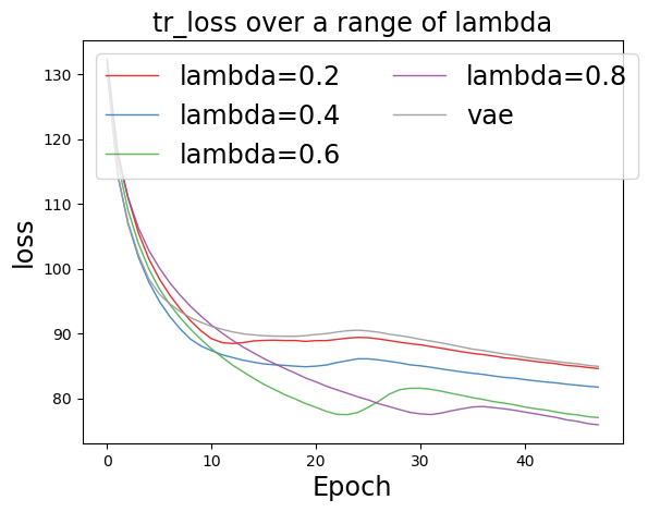
(a) train loss

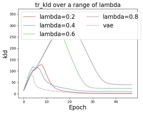
(b) train kld

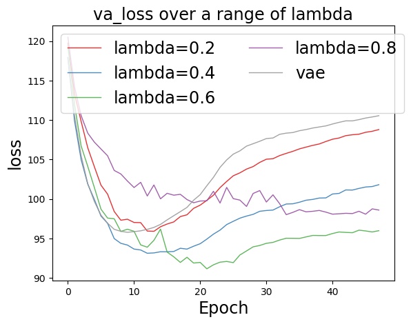
(c) validation loss

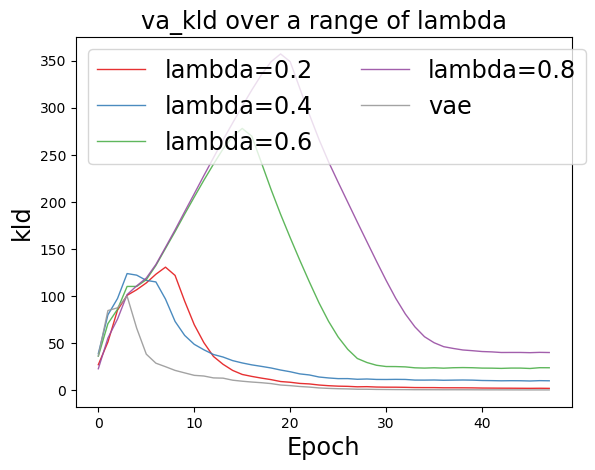
(d) validation kld

Figure 4: Training and Validation KL divergence and sequential loss for PTB using Cholesky Neural Copula with different copula density weights $\lambda$. It is obvious that the optimal $\lambda$ plays a huge role in alleviating the posterior collapse problem and does not result in overfitting as VAE does. Models are trained using 1-layer LSTM with 200 hidden units for Encoder/Decoder, in which the embedding size is 200 and the latent dimension is 32.

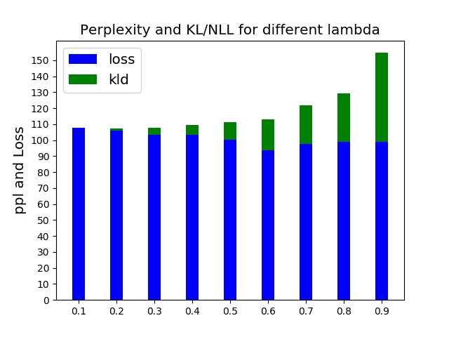
Figure 5: Reconstruction loss, KL divergence, and PPL (sum of loss and KL) on PTB. When we gradually increase $\lambda$, the KL divergence increases and the test reconstruction will decrease.

5.2 Experimental Setup

We set up a similar experimental condition as in  Bowman et al. (2015); Xiao et al. (2018); Yang et al. (2017); Xu and Durrett (2018). We use LSTM as our encoder-decoder model, where the number of hidden units for each hidden state is set to 512. The word embedding size is 512. And, the number of dimension for latent codes is set to 32. For both encoder and decoder, we use a dropout layer for the initial input, whose dropout rate is $\alpha=0.5$. Then, for inference, we pass the final hidden state to a linear layer following a Batch Normalizing Ioffe and Szegedy (2015) layer to get reparameterized samples from $\prod_{i}q(z_{i}|x)$ and from Gaussian copula $C_{\Sigma}$. For the training stage, the maximum vocabulary size for all inputs are set to 20000, and the maximum sequence length is set to 200. Batch size is set to 32, and we train for 30 epochs for each dataset, where we use the Adam stochastic optimization Kingma and Ba (2014) whose learning rate is $r=10^{-3}$.

We use kl annealing Bowman et al. (2015) during training. We also observe that the weight of log copula density is the most important factor which determines whether our model avoids the posterior collapse problem. We hyper tuned this parameter in order to find the optimal one.

5.3 Language Modeling Comparison

Model	NLL	KL	PPL
LSTM-LM Yang et al. (2017)	116.2	-	104.2
VAE Bowman et al. (2015)	105.2	1.74	121
vmf-VAE Xu and Durrett (2018)	96.0	5.7	79.6
VAE-NF	96.8	0.87	82.9
non-diag-VAE	105.1	4.9	121.0
copula-VAE(cho) $\lambda=0.4$	92.2	7.3	67.2

Table 3: Variational language modeling on PTB

Model	NLL	KL	PPL
VAE Bowman et al. (2015)	197.1	0.03	58.2
vmf-VAE Xu and Durrett (2018)	198.0	6.4	59.3
VAE-NF	200.4	0.1	62.5
non-diag-VAE	198.3	4.7	59.7
copula-VAE(cho) $\lambda=0.5$	187.7	10.0	48.0

Table 4: Variational language modeling on Yelp Reviews 13

Model	NLL	KL	PPL
VAE Bowman et al. (2015)	351.6	0.3	81.6
vmf-VAE Xu and Durrett (2018)	359.3	17.9	89.9
VAE-NF	353.8	0.1	83.0
lagging-VAE He et al. (2018)	326.6	6.7	64.9
non-diag-VAE	352.2	5.7	82.3
copula-VAE(cho) $\lambda=0.5$	344.2	15.4	74.4

Table 5: Variational language modeling on Yahoo

5.3.1 Comparison with other Variational models

We compare the variational language modeling results over three datasets. We show the results for Negative log-likelihood (NLL), KL divergence, and sample perplexity (PPL) for each model on these datasets. NLL is approximated by the evidence lower bound.

First, we observe that kl-annealing does not help alleviate the posterior collapse problem when it comes to larger datasets such as Yelp, but the problem is solved if we can maintain the latent code’s dependencies by maximizing the copula likelihood when we maximize the ELBO. We also observe that the weight $\lambda$ of log copula density affects results dramatically. All $\lambda$ produce competitive results compared with other methods. Here, we provide the numbers for those weights $\lambda$ that produce the lowest PPL. For PTB, copula-VAE achieves the lowest sample perplexity, best NLL approximation, and do not result in posterior collapse when $\lambda=0.4$. For Yelp, the lowest sample perplexity is achieved when $\lambda=0.5$.

We also compare with VAE models trained with normalizing flows Rezende and Mohamed (2015). We observed that our model is superior to VAE based on flows. It is worth noting that Wasserstein Autoencoder trained with Normalizing flow Wang and Wang (2019) achieves the lowest PPL 66 on PTB, and 41 on Yelp. However, the problem of designing flexible normalizing flow is orthogonal to our research.

5.3.2 Generation

Table 1 presents the results of text generation task. We first randomly sample $\mathbb{z}$ from $p(\mathbb{z})$, and then feed it into the decoder $p(\mathbb{x}|\mathbb{z})$ to generate text using greedy decoding. We can tell whether a model suffers from posterior collapse by examining the diversity of the generated sentences. The original VAE tends to generate the same type of sequences for different $\mathbb{z}$. This is very obvious in PTB where the posterior of the original VAE collapse to the prior completely. Copula-VAE, however, does not have this kind of issue and can always generate a diverse set of texts.

5.4 Hyperparameter-Tuning: Copula weights play a huge role in the training of VAE

In this section, we investigate the influence of log copula weight $\lambda$ over training. From Figure 5, we observe that our model performance is very sensitive to the value of $\lambda$. We can see that when $\lambda$ is small, the log copula density contributes a small part to the objective, and therefore does not help to maintain dependencies over latent codes. In this case, the model performs like the original VAE, where the KL divergence becomes zero at the end. When we increase $\lambda$, test KL becomes larger and test reconstruction loss becomes smaller.

This phenomenon is also observed in validation datasets, as shown in Figure 4. The training PPL is monotonically decreasing in general. However, when $\lambda$ is small and the dependency relationships over latent codes are lost, the model quickly overfits, as the KL divergence quickly becomes zero and the validation loss starts to increase. This further confirms what we showed in Figure 2. For original VAE models, the model first maximizes $\operatorname{\mathbb{E}}_{q(\mathbb{z}|\mathbb{x})}[p(\mathbb{x}|\mathbb{z})]$ which results in the decrease of both train and validation loss. Then, as $q(\mathbb{z}|\mathbb{x})$ can never match to the true posterior, $\operatorname{\mathbb{E}}_{q(\mathbb{z}|\mathbb{x})}[p(\mathbb{x}|\mathbb{z})]$ reaches to its ceiling which then results in the decrease of KL as it is needed to maximize the ELBO. During this stage, the LSTM decoder starts to learn how to generate texts with standard Gaussian latent variables which then causes the increase of validation loss. On the other hand, if we gradually increase the contribution of copula density by increasing the $\lambda$, the model is able to maintain the dependencies of latent codes and hence the structure of the true posterior. In this case, $\operatorname{\mathbb{E}}_{q(\mathbb{z}|\mathbb{x})}[p(\mathbb{x}|\mathbb{z})]$ will be much higher and will leverage the decrease of KL. In this case, the decoder is forced to generate texts from non-standard Gaussian latent codes. Therefore, the validation loss also decreases monotonically in general.

One major drawback of our model is the amount of training time, which is 5 times longer than the original VAE method. In terms of performance, copula-VAE achieves the lowest reconstruction loss when $\lambda=0.6$. It is clear that from Figure 5 that increasing $\lambda$ will result in larger KL divergence.

6 Conclusion

In this paper, we introduce Copula-VAE with Cholesky reparameterization method for Gaussian Copula. This approach averts Posterior Collapse by using Gaussian copula to maintain the dependency structure of the true posterior. Our results show that Copula-VAE significantly improves the language modeling results of other VAEs.

References

- Bedford et al. (2002) Tim Bedford, Roger M Cooke, et al. 2002. Vines–a new graphical model for dependent random variables. The Annals of Statistics, 30(4):1031–1068.
- Blei et al. (2003) David M Blei, Andrew Y Ng, and Michael I Jordan. 2003. Latent dirichlet allocation. Journal of machine Learning research, 3(Jan):993–1022.
- Bowman et al. (2015) Samuel R Bowman, Luke Vilnis, Oriol Vinyals, Andrew M Dai, Rafal Jozefowicz, and Samy Bengio. 2015. Generating sentences from a continuous space. CoNLL.
- Chen et al. (2012) Lu Chen, Vijay P Singh, Shenglian Guo, Ashok K Mishra, and Jing Guo. 2012. Drought analysis using copulas. Journal of Hydrologic Engineering, 18(7):797–808.
- Chen et al. (2008) Yanqing Chen, Timothy A Davis, William W Hager, and Sivasankaran Rajamanickam. 2008. Algorithm 887: Cholmod, supernodal sparse cholesky factorization and update/downdate. ACM Transactions on Mathematical Software (TOMS), 35(3):22.
- Choroś et al. (2010) Barbara Choroś, Rustam Ibragimov, and Elena Permiakova. 2010. Copula estimation. In Copula theory and its applications, pages 77–91. Springer.
- Czado (2010) Claudia Czado. 2010. Pair-copula constructions of multivariate copulas. In Copula theory and its applications, pages 93–109. Springer.
- Frey et al. (2001) Rüdiger Frey, Alexander J McNeil, and Mark Nyfeler. 2001. Copulas and credit models. Risk, 10(111114.10).
- Gelfand et al. (2000) Izrail Moiseevitch Gelfand, Richard A Silverman, et al. 2000. Calculus of variations. Courier Corporation.
- George and McCulloch (1993) Edward I George and Robert E McCulloch. 1993. Variable selection via gibbs sampling. Journal of the American Statistical Association, 88(423):881–889.
- Gilks et al. (1995) Walter R Gilks, Sylvia Richardson, and David Spiegelhalter. 1995. Markov chain Monte Carlo in practice. Chapman and Hall/CRC.
- Gregor et al. (2015) Karol Gregor, Ivo Danihelka, Alex Graves, Danilo Jimenez Rezende, and Daan Wierstra. 2015. Draw: A recurrent neural network for image generation. ICML.
- He et al. (2018) Junxian He, Daniel Spokoyny, Graham Neubig, and Taylor Berg-Kirkpatrick. 2018. Lagging inference networks and posterior collapse in variational autoencoders.
- Hochreiter and Schmidhuber (1997) Sepp Hochreiter and Jürgen Schmidhuber. 1997. Long short-term memory. Neural computation, 9(8):1735–1780.
- Hoffman et al. (2013) Matthew D Hoffman, David M Blei, Chong Wang, and John Paisley. 2013. Stochastic variational inference. The Journal of Machine Learning Research, 14(1):1303–1347.
- Ioffe and Szegedy (2015) Sergey Ioffe and Christian Szegedy. 2015. Batch normalization: Accelerating deep network training by reducing internal covariate shift. arXiv preprint arXiv:1502.03167.
- Jang et al. (2017) Eric Jang, Shixiang Gu, and Ben Poole. 2017. Categorical reparameterization with gumbel-softmax. ICLR.
- Jaworski et al. (2010) Piotr Jaworski, Fabrizio Durante, Wolfgang Karl Hardle, and Tomasz Rychlik. 2010. Copula theory and its applications, volume 198. Springer.
- Joe and Kurowicka (2011) Harry Joe and Dorota Kurowicka. 2011. Dependence modeling: vine copula handbook. World Scientific.
- Kim et al. (2018) Yoon Kim, Sam Wiseman, Andrew Miller, David Sontag, and Alexander Rush. 2018. Semi-amortized variational autoencoders. In International Conference on Machine Learning, pages 2683–2692.
- Kingma and Ba (2014) Diederik P Kingma and Jimmy Ba. 2014. Adam: A method for stochastic optimization. arXiv preprint arXiv:1412.6980.
- Kingma and Welling (2014) Diederik P Kingma and Max Welling. 2014. Auto-encoding variational bayes. stat, 1050:10.
- Kole et al. (2007) Erik Kole, Kees Koedijk, and Marno Verbeek. 2007. Selecting copulas for risk management. Journal of Banking & Finance, 31(8):2405–2423.
- Krizhevsky et al. (2012) Alex Krizhevsky, Ilya Sutskever, and Geoffrey E Hinton. 2012. Imagenet classification with deep convolutional neural networks. In Advances in neural information processing systems, pages 1097–1105.
- Marcus et al. (1993) Mitchell P Marcus, Mary Ann Marcinkiewicz, and Beatrice Santorini. 1993. Building a large annotated corpus of english: The penn treebank. Computational linguistics, 19(2):313–330.
- McNeil et al. (2005) Alexander J McNeil, Rüdiger Frey, Paul Embrechts, et al. 2005. Quantitative risk management: Concepts, techniques and tools, volume 3. Princeton university press Princeton.
- Miao et al. (2016) Yishu Miao, Lei Yu, and Phil Blunsom. 2016. Neural variational inference for text processing. In ICML.
- Nelsen (2007) Roger B Nelsen. 2007. An introduction to copulas. Springer Science & Business Media.
- Rezende and Mohamed (2015) Danilo Jimenez Rezende and Shakir Mohamed. 2015. Variational inference with normalizing flows. arXiv preprint arXiv:1505.05770.
- Shen et al. (2017) Tianxiao Shen, Tao Lei, Regina Barzilay, and Tommi Jaakkola. 2017. Style transfer from non-parallel text by cross-alignment. In NIPS.
- Suh and Choi (2016) Suwon Suh and Seungjin Choi. 2016. Gaussian copula variational autoencoders for mixed data. arXiv preprint arXiv:1604.04960.
- Tran et al. (2015) Dustin Tran, David Blei, and Edo M Airoldi. 2015. Copula variational inference. In Advances in Neural Information Processing Systems, pages 3564–3572.
- Tsukahara (2005) Hideatsu Tsukahara. 2005. Semiparametric estimation in copula models. Canadian Journal of Statistics, 33(3):357–375.
- Wainwright et al. (2008) Martin J Wainwright, Michael I Jordan, et al. 2008. Graphical models, exponential families, and variational inference. Foundations and Trends® in Machine Learning, 1(1–2):1–305.
- Wang and Wang (2019) Prince Zizhuang Wang and William Yang Wang. 2019. Riemannian normalizing flow on variational wasserstein autoencoder for text modeling. arXiv preprint arXiv:1904.02399.
- Wang and Hua (2014) William Yang Wang and Zhenhao Hua. 2014. A semiparametric gaussian copula regression model for predicting financial risks from earnings calls. In Proceedings of the 52nd Annual Meeting of the Association for Computational Linguistics (Volume 1: Long Papers), volume 1, pages 1155–1165.
- Wang and Wen (2015) William Yang Wang and Miaomiao Wen. 2015. I can has cheezburger? a nonparanormal approach to combining textual and visual information for predicting and generating popular meme descriptions. In Proceedings of the 2015 Conference of the North American Chapter of the Association for Computational Linguistics: Human Language Technologies, Denver, CO, USA. ACL.
- Xiao et al. (2018) Yijun Xiao, Tiancheng Zhao, and William Yang Wang. 2018. Dirichlet variational autoencoder for text modeling. arXiv preprint arXiv:1811.00135.
- Xu et al. (2016) Jiacheng Xu, Danlu Chen, Xipeng Qiu, and Xuangjing Huang. 2016. Cached long short-term memory neural networks for document-level sentiment classification. EMNLP.
- Xu and Durrett (2018) Jiacheng Xu and Greg Durrett. 2018. Spherical latent spaces for stable variational autoencoders. EMNLP.
- Xue-Kun Song (2000) Peter Xue-Kun Song. 2000. Multivariate dispersion models generated from gaussian copula. Scandinavian Journal of Statistics, 27(2):305–320.
- Yang et al. (2017) Zichao Yang, Zhiting Hu, Ruslan Salakhutdinov, and Taylor Berg-Kirkpatrick. 2017. Improved variational autoencoders for text modeling using dilated convolutions. ICML.
- Zhang and Singh (2006) LSVP Zhang and VP Singh. 2006. Bivariate flood frequency analysis using the copula method. Journal of hydrologic engineering, 11(2):150–164.
- Zhao et al. (2017) Tiancheng Zhao, Ran Zhao, and Maxine Eskenazi. 2017. Learning discourse-level diversity for neural dialog models using conditional variational autoencoders. ACL.