Botev and L’Ecuyer

Sampling via Splitting

Sampling Conditionally on a Rare Event via Generalized Splitting

Zdravko I. Botev UNSW Sydney, Australia, botev@unsw.edu.au Pierre L’Ecuyer Université de Montréal, Canada, and Inria–Rennes, France lecuyer@iro.umontreal.ca

We propose and analyze a generalized splitting method to sample approximately from a distribution conditional on the occurrence of a rare event. This has important applications in a variety of contexts in operations research, engineering, and computational statistics. The method uses independent trials starting from a single particle. We exploit this independence to obtain asymptotic and non-asymptotic bounds on the total variation error of the sampler. Our main finding is that the approximation error depends crucially on the relative variability of the number of points produced by the splitting algorithm in one run, and that this relative variability can be readily estimated via simulation. We illustrate the relevance of the proposed method on an application in which one needs to sample (approximately) from an intractable posterior density in Bayesian inference.

conditional distribution; Monte Carlo splitting; Markov chain Monte Carlo; rare-event

1 Introduction

We consider the problem of generating samples from a conditional distribution when the conditioning is on the occurrence of an event that has a small probability. We have a random variable $\boldsymbol{X}$ defined over a probability space $(\mathbb{R}^{d},\mathcal{B},\mathbb{P})$, where $\mathcal{B}$ can be taken as the Borel sigma-field, and $\boldsymbol{X}$ has a probability density function (pdf) $f$. We assume it is easy to sample exactly from the density $f$. The rare event on which we condition can be written in the form $B=\{S(\boldsymbol{x})\geq\gamma\}\in\mathcal{B}$ for an appropriately chosen measurable function $S:\mathbb{R}^{d}\to\mathbb{R}$ called the importance function. The conditional pdf is then

$$q(\boldsymbol{x})=\frac{f(\boldsymbol{x})\mathbb{I}\{S(\boldsymbol{x})\geq\gamma\}}{\ell(\gamma)},\quad\boldsymbol{x}=(x_{1},\ldots,x_{d})^{\top},$$ (1)

where $\mathbb{I}$ is the indicator function, and

$$\ell=\ell(\gamma)=\mathbb{P}(S(\boldsymbol{X})\geq\gamma)$$ (2)

is the appropriate (unknown) normalizing constant, which we assume is so small that estimating it via the naive acceptance-rejection method (simulate $\boldsymbol{X}\sim f$ until $S(\boldsymbol{X})\geq\gamma$) is impractical.

Sampling from a distribution conditional on a rare event has many applications. For example, suppose we want to generate $\boldsymbol{X}$ from an arbitrary density proportional to $p(\boldsymbol{x})$ for $\boldsymbol{x}\in\mathbb{R}^{d}$, for some known function $p$, and that it is too hard to generate samples directly from this density. Since $p$ is known, we may be able to find a density $f$ such that $\sup_{\boldsymbol{x}}{p(\boldsymbol{x})}/{f(\boldsymbol{x})}<\gamma$ for some constant $\gamma<\infty$. Then to generate $\boldsymbol{X}$, it suffices to generate a pair of independent random variables $\boldsymbol{X}\sim f$ and $U\sim\mathsf{U}(0,1)$ conditional on the event ${p(\boldsymbol{X})}/{f(\boldsymbol{X})}\geq\gamma U$, which is frequently a rare event (Kroese et al. 2011)[Section 14.5]. This fits our framework by taking $S((\boldsymbol{x},u))=p(\boldsymbol{x})/(f(\boldsymbol{x})u)$.

Another application is Bayesian Lasso regression (Park and Casella 2008), in which inference requires repeated simulation of a vector $\boldsymbol{\beta}$ of model parameters, conditional on the regularization constraint $\|\boldsymbol{\beta}\|_{1}<\gamma$. We give a detailed example of this in Section 5.

A third type of application occurs in the setting where we want to estimate the probability $\ell$ of the rare event and to understand under which circumstances the rare event is likely to occur. A popular method to estimate $\ell$ is importance sampling, and the optimal way to do it is to sample under a density $f$ proportional to the original density conditional on the rare event, and then adjust the estimator using a likelihood ratio (Tuffin et al. 2014, Botev and Ridder 2014, Botev et al. 2011). This also fits our framework. In this context, it can be very useful to sample from the conditional density to get insight on how the rare event occurs. For instance, in a network with unreliable links, one may want to sample random configurations of all the links conditionally on a failure of the network, to better understand what (typically) makes the network fail (Botev et al. 2014, 2012).

The sampling methods examined in this paper are based on the generalized splitting (GS) algorithm of Botev and Kroese (2012) for drawing a collection of random vectors whose distribution converges to a target distribution with pdf of the form (1). To apply GS, we first select an increasing sequence of levels $-\infty=\gamma_{0}<\gamma_{1}<\cdots<\gamma_{\tau}=\gamma$ for the importance function $S$. This can be done in pilot runs via a run (Botev and Kroese 2012). The algorithm uses a branching process that favors states $\boldsymbol{X}$ having a large value of $S(\boldsymbol{X})$ by resampling them conditional on staying above the current threshold, thus “splitting” those states into new copies, and then discarding those that do not reach the next level. At the end, the states that have reached the last level $\gamma$ are retained. This process is replicated several times independently and all the retained states are collected to form an empirical version of the target conditional distribution. There are many ways of choosing the total number of replications (or trials). For example, one can fix them in advance to a constant $n$, or one can repeat the procedure until $n$ trials have provided at least one retained state each, or until the total number of retained states is more than $t$, or until a certain computing budget (CPU time) has elapsed. In the latter case, one can either complete the current trial, or discard it, or just take the states retained so far from that trial.

There is a large variety of splitting-type or interacting particle algorithms to sample the state of a Markov chain approximately from its steady-state distribution conditional on a rare event; see for example Glasserman et al. (1999), Cérou et al. (2005, 2012), L’Ecuyer et al. (2009), Andrieu et al. (2010), Bréhier et al. (2016), and the references given there. The analysis of these algorithms consists in most cases in proving their unbiasedness when estimating the expectation of a random variable that can be nonzero only when the rare event occurs (estimating the probability of the rare event is a special case of this), and sometimes showing their asymptotic efficiency when the probability of the rare event decreases toward zero (Dean and Dupuis 2009).

In this paper, we are interested in the different problem of bounding the difference between the exact conditional distribution and the distribution obtained by picking a state from the sample returned by the splitting algorithm. We do this for some variants of the GS method of Botev and Kroese (2012). L’Ecuyer et al. (2018) proved that this method provides an unbiased estimator of the expected value of a cost function, but also showed that a state picked at random from the set of retained states at the last level does not follow the true conditional distribution in general.

On the other hand, the distance between the two distributions converges to zero when the number of replicates increases toward infinity. The aim of the present paper is to study how this convergence occurs and to establish explicit non-asymptotic (risk) bounds on the total variation (TV) error between the two distributions, their mean absolute value, and the expectation of the TV error in the case when it is a random variable. Our bounds are expressed in terms of simple mathematical expectations that can be estimated easily from the simulation output.

We provide convergence results for two versions of the GS algorithm. In both, we assume that whenever a trial returns no state from the rare event set (an empty trial), we discard it and try again. In the first version, we run GS until we have $n$ non-empty trials, for some fixed $n>0$. We prove that the TV distance between the true conditional distribution and the distribution of a state picked at random from the retained states from this GS version is bounded by $c_{1}/n$ where $c_{1}$ is an unknown constant that can be estimated from the simulation output. In the second version, we run GS until the total number of retained states exceeds $t$, for some fixed positive integer $t$. For this version, we show that the convergence rate is of the form $c_{2}(t)t^{-3/2}=\mathcal{O}(t^{-3/2})$, where the quantity $c_{2}(t)$ is bounded uniformly in $t$ and can be estimated from the simulation output. The derivation of these bounds is made possible thanks to the fact that GS produces independent trials, each one starting from a single particle, and this permits us to use results from renewal theory for our analysis.

Typically, approximate simulation from the target pdf (1) is accomplished using Markov chain Monte Carlo (MCMC) (for example, Jones and Hobert (2001), Taimre et al. (2019)). While MCMC sampling can be simple to implement, it still poses the challenge of analyzing its output and deciding how close the sampling or empirical distribution is to the desired target distribution (Jones and Hobert 2001). The reason for this difficulty is that MCMC generates a sequence of dependent random vectors $\boldsymbol{Y}_{1},\boldsymbol{Y}_{2},\ldots$. Typical graphical diagnostic tools like autocorrelation plots are heuristics, which do not easily provide precise qualitative measure of how close the simulated random variables follow the target distribution. Also we have to choose from an infinite number of possible one-dimensional plots. In contrast, our bounds on the TV error present a more rigorous and theoretically justified convergence assessment than the autocorrelation plots typically used in MCMC.

The rest of the paper is organized as follows. In Section 2, we recall the GS algorithm used in this paper. In Section 3, we define our versions of GS used for sampling conditional on the rare event. In Section 4, we state our main new results on the convergence of the distance between the empirical and true conditional distributions, and bounds on this distance. The proofs are given in the appendix. In Section 5, we show how our methodology can be applied in a practical setting, namely to sample approximately from the posterior density of the Bayesian Lasso. In this example, we show how the non-asymptotic risk bounds can be used to assess convergence and to estimate the error committed when using GS to sample from the conditional distribution. We also compare the simulation accuracy of GS with that of the sequential Monte Carlo method (Cérou et al. 2012).

2 Background on Generalized Splitting

We recall the GS method for estimating the rare-event probability $\ell$ in (2). This method is a simple generalization of the classical multilevel splitting technique for rare-event simulation (Kahn and Harris 1951, Glasserman et al. 1999, Garvels et al. 2002, L’Ecuyer et al. 2009). Our background material here is similar to the one given in L’Ecuyer et al. (2018).

The idea of GS is to define a discrete-time Markov chain with state $\boldsymbol{Y}$, which evolves via a branching-type random mechanism that pushes it toward a state corresponding to $\{\boldsymbol{Y}\in B\}\equiv\{S(\boldsymbol{Y})\geq\gamma\}$ in (1). To estimate the (rare-event) probability (2) via GS, we first need to choose:

1. an integer $s\geq 2$, called the splitting factor, and

2. an integer $\tau>0$ and real numbers $-\infty=\gamma_{0}<\gamma_{1}<\dots<\gamma_{\tau}=\gamma$ for which

   $$\rho_{l}:=\mathbb{P}(S(\boldsymbol{Y})\geq\gamma_{l}\mid S(\boldsymbol{Y})\geq\gamma_{l-1})\approx 1/s$$

   for $l=1,\dots,\tau$ (except for $\rho_{\tau}$, which can be larger than $1/s$). These $\gamma_{l}$’s represent the $\tau$ levels of the splitting algorithm. In Section 5 we give particular choices of $s$ and $\tau$ that are relevant to our examples.

For each level $\gamma_{l}$ we construct a Markov chain whose stationary density is equal to the density of $\boldsymbol{Y}$ conditional on $S(\boldsymbol{Y})\geq\gamma_{l}$ (a truncated density), given by

$$q_{l}(\boldsymbol{y}):=f(\boldsymbol{y})\frac{\mathbb{I}\{S(\boldsymbol{y})\geq\gamma_{l}\}}{\mathbb{P}(S(\boldsymbol{Y})\geq\gamma_{l})}.$$ (3)

Note that $q_{0}=f$ and $q_{\tau}=q$. We denote by $\kappa_{l}\equiv\kappa_{l}(\cdot\mid\cdot)$ the transition kernel of this Markov chain: $\kappa_{l}(\mathrm{d}\boldsymbol{y}\mid\boldsymbol{x})$ represents the probability that the next state is in $\mathrm{d}\boldsymbol{y}$ when the current state is $\boldsymbol{x}$. There are many ways of constructing this Markov chain and $\kappa_{l}$. A practical example using Gibbs sampling will be given in Section 5.

Algorithm 1 GS Sampler 1

0:  $s$, $\tau$, $\gamma_{1},\dots,\gamma_{\tau}$

  generate a vector $\boldsymbol{Y}$ from its unconditional density $f$

  if $S(\boldsymbol{Y})<\gamma_{1}$ then

        return  $\mathcal{X}_{\tau}=\emptyset$ and $\mathring{M}=0$

  else

        $\mathcal{X}_{1}\leftarrow\{\boldsymbol{Y}\}$    {this state $\boldsymbol{Y}$ has reached at least the first level}

        for $l=2$ to $\tau$ do

              $\mathcal{X}_{l}\leftarrow\emptyset$    {list of states that have reached the level $\gamma_{t}$}

              for all $\boldsymbol{Y}\in\mathcal{X}_{l-1}$ do

                    set $\boldsymbol{Y}_{0}\leftarrow\boldsymbol{Y}$    {we will simulate $s$ steps from this state}

                    for $j=1$ to $s$ do

                          sample $\boldsymbol{Y}_{j}$ from $\kappa_{l-1}(\mathrm{d}\boldsymbol{y}\mid\boldsymbol{Y}_{j-1})$

                          if $S(\boldsymbol{Y}_{j})\geq\gamma_{l}$ then

                                add $\boldsymbol{Y}_{j}$ to $\mathcal{X}_{l}$    {this state has reached the next level}

  return  the list $\mathring{\mathcal{Y}}=\mathcal{X}_{\tau}$ of retained states and its cardinality $\mathring{M}$.

The original GS algorithm is summarized in Algorithm 1, and is also given in L’Ecuyer et al. (2018). The algorithm returns a list $\mathring{\mathcal{Y}}$ of retained states that belong to $B=\{\boldsymbol{y}:S(\boldsymbol{y})\geq\gamma\}$, as well as the size of this list. This list is a multiset, in the sense that it may contain the same state more than once. The list $\mathring{\mathcal{Y}}$ can be empty and its cardinality $\mathring{M}=0$. The o-ring symbol in the notation is a reminder that the size of the set can be zero. In the remainder of this article, we define $\mathcal{Y}$ and $M$ as the versions of $\mathring{\mathcal{Y}}$ and $\mathring{M}$, conditional on $\mathring{M}\geq 1$.

Let $\mathcal{A}$ denote a $\sigma$-algebra of Borel measurable subsets of $\mathbb{R}^{d}$. For some of our results, $\mathcal{A}$ will be a more restricted class than the Borel subsets of $\mathbb{R}^{d}$. Algorithm 1 can be used to estimate $\mathbb{P}(\boldsymbol{Y}\in A)$ for any $A\in\mathcal{A}$ via the unbiased estimator:

$$\widehat{\mathbb{P}}(A)=\mathring{H}(A)/s^{\tau-1},$$ (4)

where $\mathring{H}(A)=|\mathring{\mathcal{Y}}\cap A|$ is the number of states $\boldsymbol{Y}\in\mathring{\mathcal{Y}}$ that belong to $A$. In practice, one will replicate this algorithm several times and take the average. The unbiasedness is implied by the following lemma, proved in L’Ecuyer et al. (2018).

Lemma 2.1 (L’Ecuyer et al. (2018))

For any measurable function $\hbar:\mathbb{R}^{d}\mapsto\mathbb{R}$ and any measurable subset $A\subseteq B$, we have

$$\mathbb{E}_{\mathrm{GS}}\left[\sum_{\boldsymbol{Y}\in\mathring{\mathcal{Y}}}\hbar(\boldsymbol{Y})\mathbb{I}\{\boldsymbol{Y}\in A\}\right]=s^{\tau-1}\mathbb{E}[\hbar(\boldsymbol{Y})\mathbb{I}\{\boldsymbol{Y}\in A\}],$$ (5)

where the expectation on the left-hand-side is with respect to $\mathring{\mathcal{Y}}$ from Algorithm 1 and the expectation on the right-hand-side is with respect to the original density $f$.

By taking $\hbar$ as the identity function in (5), we obtain that $\widehat{\mathbb{P}}(A)$ in (4) is unbiased for $\mathbb{P}(A)$:

$$\textstyle\mathbb{E}_{\mathrm{GS}}[\mathring{H}(A)]=\mathbb{E}_{\mathrm{GS}}\left[\sum_{\boldsymbol{Y}\in\mathring{\mathcal{Y}}}\mathbb{I}\{\boldsymbol{Y}\in A\}\right]=s^{\tau-1}\mathbb{P}(\boldsymbol{Y}\in A),$$

and therefore

$$\mathbb{E}_{\mathrm{GS}}[\widehat{\mathbb{P}}(A)]=\mathbb{E}_{\mathrm{GS}}[\mathring{H}(A)/s^{\tau-1}]=\mathbb{P}(\boldsymbol{Y}\in A).$$

Moreover, since $\mathbb{E}_{\mathrm{GS}}[\mathring{M}]=s^{\tau-1}\mathbb{P}(\boldsymbol{Y}\in B)$ and $A\subseteq B$, we have that

$$\frac{\mathbb{E}_{\mathrm{GS}}[\mathring{H}(A)]}{\mathbb{E}_{\mathrm{GS}}[\mathring{M}]}=\mathbb{P}(\boldsymbol{Y}\in A\mid\boldsymbol{Y}\in B)=\frac{\mathbb{P}(\boldsymbol{Y}\in A)}{\mathbb{P}(\boldsymbol{Y}\in B)}.$$

3 Sampling Conditionally on a Rare Event

When estimating an expectation as in (5), an empty list $\mathring{\mathcal{Y}}$ poses no problem: the unbiased estimator just takes the value 0 in that case. But for our purpose of sampling from a conditional distribution, we insist that there are no empty sets of retained states. To make sure that the set of retained states is non-empty, we modify the original GS so that each trial returns at least one state. Whenever a GS run returns an empty list, we simply discard it and try again. This gives Algorithm 2.

Algorithm 2 GS Sampler 2

0:  $s$, $\tau$, $\gamma_{1},\dots,\gamma_{\tau}$

  repeat

        run Algorithm 1

  until $\mathring{M}>0$

  return  the list ${\mathcal{Y}}=\mathcal{X}_{\tau}$ of retained states and its cardinality ${M}=|\mathcal{Y}|$.

Does this algorithm still provide an unbiased estimator? An important observation is that if we replace $\mathring{\mathcal{Y}}$ by $\mathcal{Y}$ in (5), the equality is no longer true. That is, we get a biased estimator of the expectation on the right. However, our main goal here is not to estimate this expectation, but to sample approximately from the conditional distribution, and we will analyze methods that use Algorithm 2 for this purpose. As mentioned earlier, there are several ways of doing it. In this paper, we examine the following two versions: (a) run a fixed number $n$ of iid replicates of Algorithm 2 and (b) perform replicates until there are more than $t$ retained states in total. These two approaches are detailed in Algorithms 3 and 4, respectively. In both cases, at the end we collect all the retained states in a multiset $\mathcal{Y}_{\cup}$. For the first version the cardinality of the returned set $\mathcal{Y}_{\cup}$ is at least $n$, whereas in the second case it is at least $t$ and $N(t)$ is the (random) number of calls to Algorithm 2. We summarize these two versions as follows.

Algorithm 3 Sampling an empirical distribution from $n$ iid non-empty GS replications

0:  $s,\tau,\gamma_{1},\dots,\gamma_{\tau}$ and $n$

  for $i=1,\ldots,n$ do

        run Algorithm 2 to obtain the list ${\mathcal{Y}}_{i}$ of size $M_{i}$

  return  the empirical distribution $\widehat{\mathbb{Q}}_{n}$ of the states in the set $\mathcal{Y}_{\cup}:=\mathcal{Y}_{1}\cup\cdots\cup\mathcal{Y}_{n}$

Algorithm 4 Sampling an empirical distribution with more than $t$ retained states

0:  $s,\tau,\gamma_{1},\dots,\gamma_{\tau}$ and $t$

  $i\leftarrow 0$ and $T_{0}\leftarrow 0$

  repeat

        $i\leftarrow i+1$

        run Algorithm 2 to obtain the list $\mathcal{Y}_{i}$ and its cardinality $M_{i}$

        $T_{i}\leftarrow T_{i-1}+M_{i}$

  until $T_{i}>t$

  return  $N(t)\leftarrow i$ and the empirical distribution $\widehat{\mathbb{Q}}_{N(t)}$ of the set of states $\mathcal{Y}_{\cup}:=\mathcal{Y}_{1}\cup\cdots\cup\mathcal{Y}_{N(t)}$

Note that $\widehat{\mathbb{Q}}_{n}$ (or $\widehat{\mathbb{Q}}_{N(t)}$) is a random distribution; it is the distribution conditional on $\mathcal{Y}_{\cup}$. The unconditional distribution of a state obtained by generating $\mathcal{Y}_{\cup}$ and then selecting one state randomly from $\mathcal{Y}_{\cup}$ is also of interest: this is the (a priori) distribution of a state sampled from $\widehat{\mathbb{Q}}_{n}$ (or $\widehat{\mathbb{Q}}_{N(t)}$), but before we run the GS algorithm to construct $\mathcal{Y}_{\cup}$. We will denote these two unconditional distributions by

$$\mathbb{Q}_{n}(A):=\mathbb{E}[\widehat{\mathbb{Q}}_{n}(A)]\quad\textrm{(for Algorithm~{}\ref{algo:n iid})}$$

and

$$\overline{\mathbb{Q}}_{t}(A):=\mathbb{E}[\widehat{\mathbb{Q}}_{N(t)}(A)]\quad\textrm{(for Algorithm~{}\ref{algo:until t})}$$

for all $A\in\mathcal{A}$, where the expectation is with respect to the realization of $\mathcal{Y}_{\cup}$. We saw earlier that

$$\frac{\mathbb{E}[\mathring{H}(A)]}{\mathbb{E}[\mathring{M}]}=\mathbb{P}(\boldsymbol{Y}\in A\mid\boldsymbol{Y}\in B).$$

Now let $H(A)=|\mathcal{Y}\cap A|$ be the number of states returned by Algorithm 2 that belong to $A$. We have $\mathbb{E}[{H}(A)]=\mathbb{E}[\mathring{H}(A)\,|\,\mathring{M}>0]=\mathbb{E}[\mathring{H}(A)]/\mathbb{P}(\mathring{M}>0)$. Likewise, $\mathbb{E}[M]=\mathbb{E}[\mathring{M}]/\mathbb{P}(\mathring{M}>0)$. Therefore,

$$\frac{\mathbb{E}[{H}(A)]}{\mathbb{E}[{M}]}=\frac{\mathbb{E}[\mathring{H}(A)]}{\mathbb{E}[\mathring{M}]}=\mathbb{P}(\boldsymbol{Y}\in A\mid\boldsymbol{Y}\in B).$$

We also know that $\widehat{\mathbb{Q}}_{n}(A)$ and $\widehat{\mathbb{Q}}_{N(t)}(A)$ converge with probability one to $\mathbb{E}[{H}(A)]/\mathbb{E}[{M}]$ when $n\to\infty$ and when $t\to\infty$, respectively, from the strong law of large numbers applied to the numerator and the denominator. Thus, they converge almost surely to the desired conditional probability $\mathbb{Q}(A):=\mathbb{P}(\boldsymbol{Y}\in A\mid\boldsymbol{Y}\in B)$.

4 Convergence Analysis

We now analyze the convergence of the empirical distribution of the retained states, $\widehat{\mathbb{Q}}_{n}$ (or $\widehat{\mathbb{Q}}_{N(t)}$), as well as its expected (i.e., unconditional on $\mathcal{Y}_{\cup}$) version $\mathbb{Q}_{n}$ (or $\overline{\mathbb{Q}}_{t}$), to the true conditional distribution $\mathbb{Q}$. The aim is to obtain non-asymptotic or risk bounds on the distance between $\mathbb{Q}$ and the empirical distribution, and its expected (unconditional) version. For a given class $\mathcal{A}$ of measurable sets, we consider the three error criteria:

1. The TV error between the expected (unconditional) distribution $\mathbb{Q}_{n}$ and $\mathbb{Q}$, that is:

   $$\sup_{A\in\mathcal{A}}\left|\mathbb{Q}_{n}(A)-\mathbb{Q}(A)\right|\;.$$

   This error measures the size of the “bias” of $\widehat{\mathbb{Q}}_{n}$ as an estimator of the true $\mathbb{Q}$.

2. The worst-case mean absolute error of the conditional distribution $\widehat{\mathbb{Q}}_{n}$, defined as:

   $$\sup_{A\in\mathcal{A}}\mathbb{E}\left|\widehat{\mathbb{Q}}_{n}(A)-\mathbb{Q}(A)\right|\;.$$

3. The (random) TV error, $\sup_{A\in\mathcal{A}}\left|\widehat{\mathbb{Q}}_{n}(A)-\mathbb{Q}(A)\right|$, of the conditional distribution $\widehat{\mathbb{Q}}_{n}$, and its expected value:

   $$\mathbb{E}\sup_{A\in\mathcal{A}}\left|\widehat{\mathbb{Q}}_{n}(A)-\mathbb{Q}(A)\right|\;.$$

By permuting the positions of the expectation, absolute value function, and the supremum ($\sup|\mathbb{E}[\cdot]|\rightarrow\sup\mathbb{E}|\cdot|\rightarrow\mathbb{E}\sup|\cdot|$), we find that the three error criteria dominate each other as follows:

$$\overbrace{\mathbb{E}\sup_{A\subseteq\mathcal{A}}|\widehat{\mathbb{Q}}_{n}(A)-\mathbb{Q}(A)|}^{\textrm{expected TV error}}~{}\geq~{}\sup_{A\subseteq\mathcal{A}}\overbrace{\mathbb{E}|\widehat{\mathbb{Q}}_{n}(A)-\mathbb{Q}(A)|}^{\textrm{mean absolute error}}~{}\geq~{}\overbrace{\sup_{A\subseteq\mathcal{A}}|\mathbb{E}[\widehat{\mathbb{Q}}_{n}(A)]-\mathbb{Q}(A)|}^{\textrm{TV error}}\;.$$

In other words, the expected TV error is the most stringent of these three errors. In fact, the (expected) TV error of the empirical distribution is so stringent that it does not converge, unless the class of sets $\mathcal{A}$ is restricted. To ensure convergence, in Section 4.2 we will take $\mathcal{A}$ to be a restricted class of subsets. In contrast, the TV and mean absolute errors do not require any restrictions on the class $\mathcal{A}$ and for these error criteria we simply take $\mathcal{A}$ to be the class of all Borel subsets of $\mathbb{R}^{d}$.

4.1 Convergence of Total Variation and Mean Absolute Errors

Let $m:=\mathbb{E}[M]$ and $\mathbb{V}\mathrm{ar}(M)$ denote the expectation and variance of $M$, which is the output of either Algorithm 3, or Algorithm 4. In this section, we state theorems giving non-asymptotic bounds on the TV error and the (worst-case) mean absolute error. The proofs of the following results are in the appendix.

Theorem 4.1 (Sampling via $n$ iid runs of GS)

The TV error is bounded as

$$\sup_{A}|\mathbb{Q}_{n}(A)-\mathbb{Q}(A)|\leq{c_{1}}{n^{-1}}$$

where $c_{1}:=\left({\mathbb{V}\mathrm{ar}(M)+\sqrt{\mathbb{V}\mathrm{ar}(M)\mathbb{E}[M^{2}]}}\right){m^{-2}}.$ The worst-case mean absolute error is bounded as

$$\sup_{A}\mathbb{E}|\widehat{\mathbb{Q}}_{n}(A)-\mathbb{Q}(A)|\leq{\tilde{c}_{1}(n)}{n^{-1/2}}$$

where $\tilde{c}_{1}(n):=\left({\sqrt{\mathbb{E}M^{2}}}+{\sqrt{3\mathbb{E}M^{4}/n}}\right)m^{-1}$ is bounded uniformly in $n$.

The terms $c_{1}$ and $\tilde{c}_{1}(n)$ in these bounds can be estimated from the simulation output.

Theorem 4.2 (Sampling until GS returns $t$ states)

In this case, the TV error is bounded as

$$\sup_{A}|\overline{\mathbb{Q}}_{t}(A)-\mathbb{Q}(A)|\leq{c_{2}(t)}{(t/m)^{-3/2}},$$

where $c_{2}(t):=\sqrt{(4/3)\mathbb{E}[M^{3}]\mathbb{E}[M^{2}]\left(m+\mathbb{E}[M^{2}]/t\right)}\;m^{-3}$ is bounded uniformly in $t$. The worst-case mean absolute error is bounded as

$$\sup_{A}\mathbb{E}|\widehat{\mathbb{Q}}_{N(t)}(A)-\mathbb{Q}(A)|\leq\tilde{c}_{2}(t)(t/m)^{-1/2},$$

where $\tilde{c}_{2}(t):=({\mathbb{E}M^{2}})^{1/2}m^{-1}+({\mathbb{E}M^{2}})m^{-3/2}t^{-1/2}$ is also uniformly bounded in $t$.

Again, the terms $c_{2}(t)$ and $\tilde{c}_{2}(t)$ can be estimated easily by simulation: it suffices to estimate ${\mathbb{E}M^{2}}$ and ${\mathbb{E}M^{3}}$ by their empirical versions. The constant $m$ in $(t/m)^{-3/2}$ could be absorbed into $c_{2}(t)$, but we choose not to do this, because we want to be able to compare $\overline{\mathbb{Q}}_{t}$ and $\mathbb{Q}_{n}$ on a common scale, where $n$ (the simulation effort of Algorithm 3) and $t/m$ (the average simulation effort of Algorithm 4 for large $t$) are the same. The key point to notice is that we get a better rate for the bound for $\overline{\mathbb{Q}}_{t}$ than for $\mathbb{Q}_{n}$.

In the next result, we obtain an improved convergence rate of $\mathcal{O}(1/t^{2})$, but at the price of introducing in the bound an $\mathcal{O}(\exp(-\omega t))$ term (for some $\omega>0$) which is hard to estimate. This term converges exponentially fast in $t$, so it is asymptotically negligible when $t\to\infty$, but it is not necessarily negligible for a given (finite) $t$. So we have an asymptotically better bound that we cannot easily estimate. In practical settings, we may prefer the $\mathcal{O}((t/m)^{-3/2})$ bound from Theorem 4.2 that we can more easily estimate to the $\mathcal{O}((t/m)^{-2})$ bound that we cannot completely estimate.

Theorem 4.3 (Sampling until GS returns $t$ states; asymptotic version)

We have

$$\sup_{A}|\overline{\mathbb{Q}}_{t}(A)-\mathbb{Q}(A)|\leq c_{3}(t/m)^{-2}+\mathcal{O}(\exp(-\omega t)),$$

where $\omega>0$ is a (typically unknown) constant and

$$c_{3}:=\frac{\mathbb{E}[M^{2}|M-1-2r|]}{2m^{3}}$$

with $r:=(\mathbb{E}M^{2}+m)/(2m)$.

This result does not include a statement about the mean absolute error, because the bounds of the mean absolute errors in Theorems 4.1 and 4.2 already converge at the optimal asymptotic rate, and thus cannot be improved.

4.2 Convergence of the Empirical Conditional Distribution $\widehat{\mathbb{Q}}_{n}$

We now examine the convergence of the TV error between the empirical distribution $\widehat{\mathbb{Q}}_{n}$ and $\mathbb{Q}$ when $n\to\infty$. This distribution is random, and any realization is discrete with finite support, so obviously it cannot converge to $\mathbb{Q}$ in TV with $\mathcal{A}$ taken as all the Borel sets, because by taking $A$ as the finite set $\mathcal{Y}_{\cup}$, we get $\widehat{\mathbb{Q}}_{n}(A)=1$ for any $n$, but $\mathbb{Q}(A)=0$ (assuming that $\mathbb{Q}$ has a density). Thus, as mentioned previously, we necessarily have to restrict the class $\mathcal{A}$. We start by giving conditions for TV convergence with probability 1 under the following restrictions on the class $\mathcal{A}$.

Suppose that one of the following two conditions holds:

1. $\mathcal{A}$ is a class with finite Vapnik-Chervonenkis (VC) dimension, or

2. $\mathcal{A}$ is the class of all convex sets in $\mathbb{R}^{d}$, and the transition kernel in Algorithm 1 has a probability density $\kappa_{l}(\boldsymbol{y}\mid\boldsymbol{x})$.

Theorem 4.4 (Almost-Sure TV Convergence)

Under Assumption 4.2, we have almost sure TV convergence:

$$\sup_{A\subseteq\mathcal{A}}|\widehat{\mathbb{Q}}_{n}(A)-\mathbb{Q}(A)|\longrightarrow 0\quad\textrm{ with probability 1 when }n\to\infty.$$

The notion of VC dimension is discussed for example by Vapnik (2013). Roughly speaking, it measures the flexibility of a class of subsets to correctly classify data defined over $\mathbb{R}^{d}$, and in our context it measures the complexity of the class of sets $\mathcal{A}$. Sets with higher VC dimension are more complex.

Note that the class of convex sets has an infinite VC dimension, which is why the second option in Assumption 4.2 requires the extra regularity condition on the transition kernel. This condition will be satisfied if $\kappa_{l}$ is the transition kernel of a Gibbs sampler, but will not be satisfied for the kernel of a Metropolis-Hastings sampler (Kroese et al. 2011, Equation 6.3, Page 226). Note that the condition does not require that we have a closed form (simple) formula for the transition density $\kappa_{l}(\boldsymbol{y}\mid\boldsymbol{x})$. It only requires that it exists.

Our next result (proof in Appendix 7.5) provides bounds on the expected TV error of the empirical distribution, where $\mathcal{A}$ is a class of sets with a finite VC dimension.

Theorem 4.5 (Bound on Expected TV for Empirical Distribution)

Suppose the class $\mathcal{A}$ has finite VC dimension $v$. Then, the expected TV error made by using the empirical distribution $\widehat{\mathbb{Q}}_{n}$ as an approximation of $\mathbb{Q}$ is bounded as follows:

$$\mathbb{E}\sup_{A\in\mathcal{A}}|\widehat{\mathbb{Q}}_{n}(A)-\mathbb{Q}(A)|\leq\frac{\sqrt{\mathbb{V}\mathrm{ar}(M)}}{m\sqrt{n}}+\frac{2\sqrt{v\,\ln(2n)\,\mathbb{E}[M^{2}\ln M]}}{m\sqrt{n}}\;\psi_{1}(v,n),$$

where

$$\psi_{1}=\psi_{1}(v,n):=\sqrt{\frac{(\ln(2)+v+v\ln(2n/v))\mathbb{E}[M^{2}]}{v\ln(2n)\mathbb{E}[M^{2}\ln M]}+\frac{1}{\ln(2n)}}<\infty$$

is bounded uniformly in $(v,n,\tau)$.

As an example, let $[\boldsymbol{a},\boldsymbol{b}]=\{\boldsymbol{y}\in\mathbb{R}^{d}:\boldsymbol{a}\leq\boldsymbol{y}\leq\boldsymbol{b}\}$ represent a rectangle in $\mathbb{R}^{d}$, and suppose $\mathcal{A}$ is the class of all rectangles in $\mathbb{R}^{d}$. Then $v=2d$ (Sauer 1972). If $\boldsymbol{a}=-\boldsymbol{\infty}$, that is, $\mathcal{A}$ as the class of one-sided intervals of the form $[-\boldsymbol{\infty},\boldsymbol{b}]$, then $v=d+1$. In this case, the previous theorem can provide a bound on the expected value of the Kolmogorov-Smirnov statistic:

$$\mathrm{ks}(n):=\mathbb{E}\left[\;\sup_{\boldsymbol{x}\in\mathbb{R}^{d}}\left|\widehat{\mathbb{Q}}_{n}(\boldsymbol{X}\leq\boldsymbol{x})-\mathbb{Q}(\boldsymbol{X}\leq\boldsymbol{x})\right|\;\right].$$ (6)

We will use this type of error bound in Section 5.2 when we assess the quality of our approximate sampling from a Bayesian posterior.

Using the metric entropy of the class $\mathcal{A}$, it is also possible to obtain a bound without the logarithmic growth term $\ln(n)\ln(M)$ in Theorem 4.5, and to get an expected TV bound that depends solely on the relative second moment of $M$.

Theorem 4.6 (Second Bound on Expected TV for Empirical Distribution)

Let $\tau$ be the number of levels in Algorithm 1 with splitting factor $s$ and suppose that $\mathcal{A}$ has VC dimension $v<\infty$. Then the empirical distribution $\widehat{\mathbb{Q}}_{n}$ satisfies:

$$\mathbb{E}\sup_{A\in\mathcal{A}}|\widehat{\mathbb{Q}}_{n}(A)-\mathbb{Q}(A)|\leq\frac{\sqrt{\mathbb{V}\mathrm{ar}(M)}}{m\sqrt{n}}+\frac{(s+1)4\sqrt{v\;\mathbb{E}[M^{2}]}}{m\sqrt{n}}\psi_{2}(\tau,v,n,s),$$

where

$$\psi_{2}=\psi_{2}(\tau,v,n,s):=\sum_{k=1}^{\lceil\tau+\log_{s}\sqrt{n}\rceil}\frac{1}{s^{k}}\left(\frac{\ln 2}{2nv}+\frac{1+\ln(v+1)}{v}+1+\ln(2s^{2k})\right)^{1/2}~{}<~{}\infty$$

is bounded uniformly in $(\tau,v,n,s)$.

Unfortunately, as we shall see in Section 5.2, the constant $\psi_{2}$ in this bound is much larger than $\psi_{1}$ in Theorem 4.5. As a result, $n$ has to be impractically large for the above bound to beat the simpler bound in Theorem 4.5. Nevertheless, the result is still of theoretical interest as it shows that the rate of convergence in expectation of the TV distance can be improved from $\mathcal{O}(\ln(n)/\sqrt{n})$ to the canonical rate of $\mathcal{O}(1/\sqrt{n})$. In addition, the term $\mathbb{E}[M^{2}\ln M]/m^{2}$ in Theorem 4.5 does not appear in Theorem 4.6.

Remark 4.7 (Simplifications due to Existence of a Density)

If the transition density $\kappa_{l}(\boldsymbol{x}|\boldsymbol{y})$ is available in closed form and easily evaluated, we can do much better by dropping the restrictions that the class $\mathcal{A}$ has a finite VC dimension. Instead, if $\kappa(\boldsymbol{x}|\boldsymbol{y})\equiv\kappa_{\tau}(\boldsymbol{x}|\boldsymbol{y})$ is a transition density with stationary pdf $q$, then we can define the empirical density:

$$\hat{q}_{n}(\boldsymbol{x}):=\frac{1}{T_{n}}\sum_{\boldsymbol{Y}\in\mathcal{Y}_{\cup}}\kappa(\boldsymbol{x}|\boldsymbol{Y}),$$

so that we can use Sheffé’s identity (Devroye and Lugosi 2001, Theorem 5.1) to simplify the uniform deviation over the class $\mathcal{B}$ of Borel measurable sets:

$$2\sup_{A\in\mathcal{B}}\left|\int_{A}\hat{q}_{n}(\boldsymbol{x})\mathrm{d}\boldsymbol{x}-\mathbb{Q}(A)\right|=\int_{\mathbb{R}^{d}}|\hat{q}_{n}(\boldsymbol{x})-q(\boldsymbol{x})|\mathrm{d}\boldsymbol{x}$$

Therefore, the bound on the expected TV distance simplifies as follows:

$$\begin{split}2\mathbb{E}\left[\sup_{A\in\mathcal{B}}\left|\int_{A}\hat{q}_{n}(\boldsymbol{x})\mathrm{d}\boldsymbol{x}-\mathbb{Q}(A)\right|\right]&\leq\mathbb{E}\int_{\mathbb{R}^{d}}\left|\frac{1}{n\bar{M}_{n}}\sum_{\boldsymbol{Y}\in\mathcal{Y}_{\cup}}\kappa(\boldsymbol{x}|\boldsymbol{Y})-\frac{1}{nm}\sum_{\boldsymbol{Y}\in\mathcal{Y}_{\cup}}\kappa(\boldsymbol{x}|\boldsymbol{Y})\right|\mathrm{d}\boldsymbol{x}\\ &\qquad+\mathbb{E}\int_{\mathbb{R}^{d}}\left|\frac{1}{nm}\sum_{\boldsymbol{Y}\in\mathcal{Y}_{\cup}}\kappa(\boldsymbol{x}|\boldsymbol{Y})-q(\boldsymbol{x})\right|\mathrm{d}\boldsymbol{x}\\ &\leq\frac{1}{m\sqrt{n}}\Big{(}\sqrt{\mathbb{V}\mathrm{ar}(M)}+\textstyle\sqrt{\int_{\mathbb{R}^{d}}\mathbb{V}\mathrm{ar}(\kappa(\boldsymbol{x}|\boldsymbol{Y}))\mathrm{d}\boldsymbol{x}}\Big{)}\;.\end{split}$$

Thus, provided the integrated variance $\int\mathbb{V}\mathrm{ar}(\kappa(\boldsymbol{x}|\boldsymbol{Y}))\mathrm{d}\boldsymbol{x}$ can be estimated easily, this bound can be used as a simpler alternative to Theorem 4.5. We do not pursue this possibility further in this article.

5 Numerical Example: Bayesian Lasso

In this section we consider an application of the splitting sampler in Algorithm 2 to the problem of posterior simulation in Bayesian inference. We estimate the bounds in Theorems 1 to 6 in order to assess the convergence of Algorithms 3 and 4. This convergence assessment can be used to either assess whether any Bayesian credible intervals are reliably estimated from the simulation output, or to rank the performance of implementations that use different Markov chain kernels $\kappa_{l}$ (the Markov chain that yields the smallest TV error will be the preferred one).

5.1 Approximate Posterior Simulations via Splitting

One of the simplest and most widely used linear regression models for data $\boldsymbol{y}=(y_{1},\ldots,y_{n^{\prime}})^{\top}$ is the Bayesian Lasso (Park and Casella 2008), in which the point-estimator of the regression coefficient $\boldsymbol{\beta}=(\beta_{1},\dots,\beta_{d})^{\top}\in\mathbb{R}^{d}$ is defined as the minimizer of the constrained least squares problem:

$$\min_{\boldsymbol{\beta}}\|\boldsymbol{y}-\mathbf{X}\boldsymbol{\beta}\|^{2}_{2},\qquad\textrm{subject to }\|\boldsymbol{\beta}\|_{1}\leq\gamma,$$

where: (1) $\mathbf{X}$ is a matrix with $d$ columns (predictors); (2) the term $\|\boldsymbol{\beta}\|_{1}=|\beta_{1}|+\cdots+|\beta_{d}|$ is the least absolute shrinkage and selection operator (Lasso); and (3) $\gamma\geq 0$ is the Lasso regularization parameter. In a Bayesian linear regression, one wishes to estimate the posterior distribution of the parameters $(\boldsymbol{\beta},\sigma^{2})$, that is, the distribution of $(\boldsymbol{\beta},\sigma^{2})$ conditional on the data $\boldsymbol{y}$ and the constraint $\|\boldsymbol{\beta}\|_{1}\leq\gamma$. Since this posterior distribution is intractable, one typically approximates it by sampling random pairs $(\boldsymbol{\beta},\sigma)$ from the posterior pdf:

$$\begin{split}q(\boldsymbol{\beta},\sigma|\boldsymbol{y},\gamma)&~{}\varpropto~{}\phi(\boldsymbol{y}-\mathbf{X}\boldsymbol{\beta};\sigma^{2}\mathbf{I})\;\sigma^{-2}\;\mathbb{I}\{\|\boldsymbol{\beta}\|_{1}\leq\gamma\}\times d!/{(2\gamma)^{d}}\;,\end{split}$$ (7)

where: a) $\phi(\boldsymbol{x};\Sigma)$ denotes the multivariate normal pdf with mean zero and covariance matrix $\Sigma$ evaluated at $\boldsymbol{x}$; b) the factor $\sigma^{-2}$ results from using an uninformative prior for the scale $\sigma$, and c) ${\mathbb{I}\{\|\boldsymbol{\beta}\|_{1}\leq\gamma\}}\times d!/{(2\gamma)^{d}}$ is the prior of $\boldsymbol{\beta}$, uniform over the feasible set. Note that, unlike the more common Laplace prior used in the Bayesian Lasso (Park and Casella 2008), here the prior enforces the constraint on $\boldsymbol{\beta}$ directly.

To sample a new state $(\boldsymbol{\beta}_{k},\sigma_{k})$ during the course of splitting, we need to simulate from a transition density $\kappa_{l}((\sigma_{k},\boldsymbol{\beta}_{k})\,|\,(\sigma_{k-1},\boldsymbol{\beta}_{k-1}))$, which is stationary with respect to the density (3). We simulate a move from $(\sigma_{k-1},\boldsymbol{\beta}_{k-1})$ to $(\sigma_{k},\boldsymbol{\beta}_{k})$ as follows. Given $\boldsymbol{\beta}_{k-1}$, we sample

$$(1/\sigma^{2}_{k})\ \sim\ \mathsf{Gamma}((n^{\prime}+1)/2,\|\boldsymbol{y}-\mathbf{X}\boldsymbol{\beta}_{k-1}\|^{2}_{2}/2),$$

which is the gamma distribution with mean $(n^{\prime}+1)/\|\boldsymbol{y}-\mathbf{X}\boldsymbol{\beta}_{k-1}\|^{2}_{2}$ and shape parameter $(n^{\prime}+1)/2$. Given $(\sigma_{k},\boldsymbol{\beta}_{k-1})$, we simulate $\boldsymbol{\beta}_{k}$ via a “hit-and-run” Gibbs sampler (Kroese et al. 2011, Page 240). In other words, the new state is $\boldsymbol{\beta}_{k}=\boldsymbol{\beta}_{k-1}+\lambda\boldsymbol{d}$, where $\boldsymbol{d}$ is a point uniformly distributed on the surface of the $d$-dimensional unit hyper-sphere, and the scalar $\lambda$ is simulated according to:

$$(\lambda\,|\,\boldsymbol{d},\sigma_{k},\boldsymbol{\beta}_{k-1})~{}\sim~{}\varphi(\lambda\,|\,\boldsymbol{d},\sigma_{k},\boldsymbol{\beta}_{k-1})~{}:=~{}\frac{q(\boldsymbol{\beta}_{k-1}+\lambda\boldsymbol{d},\sigma_{k}\,|\,\boldsymbol{y},\gamma)}{\int q(\boldsymbol{\beta}_{k}+\xi\boldsymbol{d},\sigma_{k}\,|\,\boldsymbol{y},\gamma)\mathrm{d}\xi}\;.$$

The conditional pdf $\varphi(\lambda\,|\,\boldsymbol{d},\sigma,\boldsymbol{\beta}_{k-1})$ is a univariate truncated normal, which can be simulated easily (Botev and L’Ecuyer 2017).

As a concrete illustration we use the “diabetes dataset” (Park and Casella 2008), consisting of $n^{\prime}=442$ patients. For each patient, we have a record of $d=10$ predictor variables (age, sex, body mass index, and 7 blood serum measurements, so that $\mathbf{X}$ is a matrix of size $442\times 10$), and a response variable, which measures the severity of nascent diabetes. We fix $\gamma=1200$, which corresponds to the Lasso regularization parameter value used by Park and Casella (2008).

To simulate from the Bayesian posterior (7) we ran Algorithm 2 with splitting factor $s=100$ and $n=10^{4}$ using the following $\tau=4$ levels: $(\gamma_{1},\gamma_{2},\gamma_{3},\gamma_{4})=(1907,1368,1230,1200)$ to obtain the multiset $\mathcal{Y}_{\cup}$. The first three levels were chosen so that $\rho_{j}\approx 0.01$ for $j=1,\ldots,3$. The values for $\tau,\gamma_{1},\ldots,\gamma_{\tau}$ were selected by running the adaptive pilot algorithm in (Botev et al. 2012)[Algorithm 4]. The marginal empirical distribution of each coefficient $\beta_{j}$ is illustrated in Figure 1 as a boxplot.

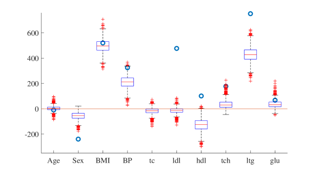
Figure 1: Empirical marginal distributions of the ten coefficients $\beta_{j}$ corresponding to the ten predictors, sampled approximately from (7). For comparison, the unconstrained (ordinary) least squares solution for each $\beta_{j}$ is displayed as a circle.

5.2 Convergence Assessment via Theoretical Bounds

Using the output of Algorithm 2 from the previous section we calculated point estimates of the unknown terms, $c_{1},\tilde{c}_{1}(n),c_{2}(t),\tilde{c}_{2}(t),c_{3},\psi_{1},\psi_{2}$, appearing in Theorems 1 through 6. Note that all the unknown terms depend on moments of $M$. For example, some of the point-estimates of the moments of $M$ are $(\mathbb{E}M,\mathbb{E}M^{2})\approx(5.9,71)$. Figure 2 shows the estimates of $c_{1}/n$, $c_{2}(t)\,(t/m)^{-3/2}$, and $c_{3}\,(t/m)^{-2}$, which bound the TV error (see Theorems 1 to 3), on a common scale with $t=n\times 5.9$ (since $m=\mathbb{E}[M]\approx 5.9$).

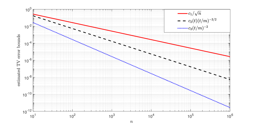
Figure 2: Comparison of three bounds on the TV error, $c_{1}/\sqrt{n},\;c_{2}(t)\times(t/m)^{-3/2}$, and $c_{3}\times(t/m)^{-2}$, where $t=n\times m$.

There is one major take-home message from Figure 2, namely, that Algorithm 4 (sampling to exceed $t$ states) simulates more closely (in terms of TV error) from the target distribution $\mathbb{Q}$ than Algorithm 3 ($n$ iid non-empty replications). Of course, the downside of using Algorithm 4 is that the number of trials, $N(t)$, is random (with expectation $t/m$ for large $t$).

In addition, reading off from Figure 2 we can see that if we run Algorithm 4 with $t>5.9\times 10^{3}$, then the TV error between $\overline{\mathbb{Q}}_{t}$ and $\mathbb{Q}$ is estimated as less than $10^{-3}$ using the non-asymptotic bound $c_{2}(t)(t/m)^{-3/2}$ and as less than $10^{-5}$ using the asymptotic bound $c_{3}(t/m)^{-2}$ (it is asymptotic, because we ignored the asymptotically negligible $\mathcal{O}(\exp(-\omega t))$ term in Theorem 4.3).

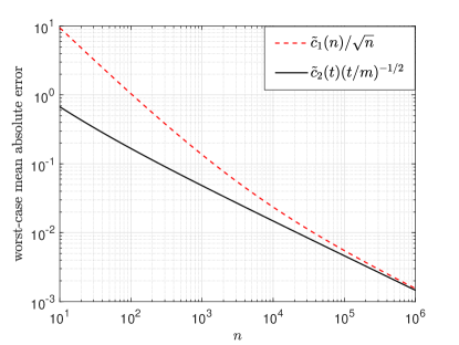
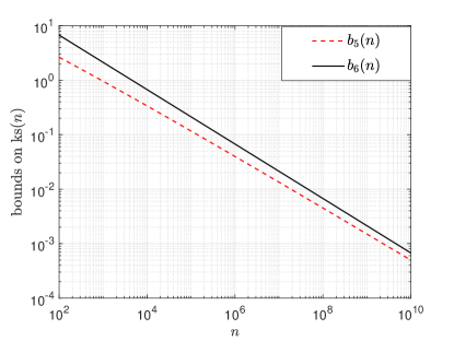
Figure 3: Left: estimates of the worst-case mean absolute error; Right: estimates of the expected TV error.

As for the mean absolute error, the left pane of Figure 3 shows the estimated bounds $\tilde{c}_{1}(n){n}^{-1/2}$ and $\tilde{c}_{2}(t)(t/m)^{-1/2}$ given in Theorems 4.1 and 4.2, respectively, using $t=n\times m$.

It is clear that the bound $\tilde{c}_{2}(t)(t/m)^{-1/2}$ is always smaller. Note that both bounds are asymptotically equivalent to first order — as $n$ becomes larger, the two bounds converge to each other. Based on the mean absolute error, in this example we again conclude that Algorithm 4 (sample more than $t=m\times n$ states) is a better performing sampler than Algorithm 3 ($n$ iid non-empty runs).

Next, we apply the results of Theorems 4.5 and 4.6 to bound the expectation of the Kolmogorov-Smirnov statistic, $\mathrm{ks}(n)$, given in (6). Let $b_{5}(n)$ and $b_{6}(n)$ be the upper bounds on (6) derived in Theorems 4.5 and 4.6, respectively (here $v=d+1=11$). The right pane of Figure 3 shows the estimated bounds on the value of $\mathrm{ks}(n)$. There are a number of observations to be made.

First, we can see that for the range of the plot, $b_{5}(n)=\mathcal{O}(\ln(n)/\sqrt{n})$ yields a better risk bound than $b_{6}(n)=\mathcal{O}(1/\sqrt{n})$ (despite the superior convergence rate of $b_{6}$). This is because, as mentioned previously, the constant $\psi_{2}$ in Theorem 4.6 is much larger than $\psi_{1}$ in Theorem 4.5. In fact, the cross-over for which ultimately $b_{6}(n)<b_{5}(n)$ happens for $n>10^{19}$ (not shown on Figure 3).

Second, from the right pane of Figure 3 we can see that the expectation of the Kolmogorov-Smirnov statistic is indeed the most stringent error criteria, because we need a very large $n$ to guarantee an acceptably small error (at least $n>10^{7}$ to make $b_{5}(n)$ smaller than $10^{-2}$).

Third, we observe that since the transition kernel, $\kappa_{l}$, has a density (it is the transition pdf of a Gibbs Markov chain), Theorem 4.4 ensures the almost sure convergence of the empirical TV uniformly over the class $\mathcal{A}$ of all convex subsets, that is, $\sup_{A\in\mathcal{A}}|\widehat{\mathbb{Q}}_{n}(A)-\mathbb{Q}(A)|\longrightarrow 0$ with probability one.

Finally, we note that our convergence results do not theoretically quantify the speed of convergence of the Markov chains, induced by the kernels $\kappa_{l}$. This dynamics is captured by the moments of $M$, which we estimate empirically, but not theoretically. To analyze theoretically the growth of the moments of $M$ will require an analysis of the speed of convergence of all Markov chains used in Algorithm 1.

5.3 Comparison with Sequential Monte Carlo for Rare Event Estimation

In the Bayesian context, the rare-event probability $\ell(\gamma)=\mathbb{P}(\|\boldsymbol{\beta}\|_{1}\leq\gamma)$ is the normalizing constant of the posterior (7), also called the model evidence or marginal likelihood, which is of importance in model selection and inference.

From equation (4) above, we can see that an estimator of $\ell$ using $n=10^{4}$ independent runs of Algorithm 1 is $\hat{\ell}:=(\mathring{M}_{1}+\cdots+\mathring{M}_{n})/(ns^{\tau-1})$ with relative error $\sqrt{\mathbb{V}\mathrm{ar}(\mathring{M})}\big{/}(\hat{\ell}\sqrt{n})$. We obtained the estimate of $\hat{\ell}=2.4\times 10^{-8}$ with estimated relative error of $3.6\%$.

For completeness, and as a benchmark to our results, we compared the performance of Algorithm 1 with the popular sequential Monte Carlo (SMC) method for rare-event estimation of Cérou et al. (2012), as described on top of page 798, column 1. For the SMC we used the same intermediate thresholds $(\gamma_{1},\gamma_{2},\gamma_{3},\gamma_{4})=(1907,1368,1230,1200)$ (in the notation on page 798, we have $A_{k}:=\{\|\boldsymbol{\beta}\|_{1}<\gamma_{k}\}$) and a total simulation effort of $6\times 10^{6}$ particles to estimate $\ell$. This is roughly twice the average simulation effort for $n$ runs of Algorithm 1, which is approximately $n\times\sum_{k=1}^{\tau}\frac{1}{\rho_{k}}\approx 3.4\times 10^{6}$. Despite this, the relative error of the SMC estimator of $\ell$ was estimated as $12\%$, or about three times larger than the relative error of $\hat{\ell}$.

The observation that the GS algorithm can, under certain conditions, perform better than sequential Monte Carlo methods is known and is already explained in Botev and Kroese (2012). Briefly, the GS sampler is expected to outperform standard SMC methods when the Markov chain induced by $\kappa_{l}$ converges slowly to its stationary pdf (3). Conversely, when the Markov chain at each level $l$ mixes fast (the particles follow the law of (3) almost exactly), then SMC methods are to be preferred. As previously explained (Botev and Kroese 2012), unlike standard SMC methods, the GS sampler does not have a bootstrap resampling step, which is advantageous when the transition kernel $\kappa_{l}$ fails to create enough “diversity” in the samples (bootstrap resampling reduces the diversity). This advantage, however, disappears if the Markov chains at each level are mixing fast, and as a result using a fixed number of particles at each level (Cérou et al. 2012, Page 798) leads to superior accuracy compared to using a random number of particles (as in the GS Algorithm 1).

6 Summary and Conclusions

We presented two different implementations of the generalized splitting method that can be used to simulate approximately from a conditional density in high dimensions. In the first implementation, we construct an empirical distribution $\widehat{\mathbb{Q}}_{n}$ from $n$ iid non-empty replications of the GS sampler (Algorithm 1). In the second implementation, we construct an empirical distribution $\widehat{\mathbb{Q}}_{N(t)}$ by running Algorithm 2 until we have more than $t$ states in total. In both implementations, $\widehat{\mathbb{Q}}_{n}$ and $\widehat{\mathbb{Q}}_{N(t)}$, and their respective expectations $\mathbb{Q}_{n}$ and $\overline{\mathbb{Q}}_{t}$, aim to approximate the true distribution $\mathbb{Q}$.

To assess the quality of the approximations we derived non-asymptotic bounds on three different error criteria: (1) the total variation errors of $\mathbb{Q}_{n}$ and $\overline{\mathbb{Q}}_{t}$, widely used in MCMC convergence analysis; (2) the mean absolute errors of $\widehat{\mathbb{Q}}_{n}$ and $\widehat{\mathbb{Q}}_{N(t)}$; and (3) the expected total variation error of $\widehat{\mathbb{Q}}_{n}$.

The main take-away messages are as follows. First, the GS sampler in Algorithm 4, which samples until we have more than $t$ states in total, converges faster than the GS sampler in Algorithm 3, which samples $n$ iid non-empty replications.

Second, the proposed splitting samplers provide a simple qualitative method for assessing whether they are sampling accurately from the target distribution. Any unknown constants and terms in the theoretical error estimates depend only on moments of the number $M$ of particles, which can be readily estimated from the simulation output. This allows us to make qualitative statements such as “choose $n>10^{3}$ to (approximately) obtain a total variation error of less than $10^{-3}$”, or to rank the performance of different implementations of the algorithms.

Finally, we have confirmed that, under certain conditions, generalized splitting can be more efficient than sequential Monte Carlo in estimating rare-event probabilities. This observation extends not just to estimation, but approximate sampling as well, because if an algorithm is not the most efficient in estimating a rare-event probability, then it will also not be the most efficient algorithm to simulate conditional on the rare event.

7 Proof of the Theorems

We first recall the working notation. Let $\mathcal{A}$ be a class of measurable sets. For any $A\subseteq\mathcal{A}$ and $i\geq 1$, let $M_{i}$ and $H_{i}(A)$ be the cardinalities of $\mathcal{Y}_{i}$ and of $\mathcal{Y}_{i}\cap A$. These are the realizations of $M$ and $H(A)$ for replication $i$ of Algorithm 2. Let $\bar{M}_{n}$ and $\bar{H}_{n}(A)$ be the respective averages of these $n$ realizations, and let $m:=\mathbb{E}_{\mathrm{GS}}[M]$, so that the target distribution is $\mathbb{Q}(A)=\mathbb{E}_{\mathrm{GS}}[H(A)]/m$. For simplicity of notation, unless there is ambiguity, we henceforth drop the GS subscripts from $\mathbb{E}_{\mathrm{GS}}$. When we draw an $\boldsymbol{Y}$ from $\widehat{\mathbb{Q}}_{n}$, it belongs to $A$ with probability $\bar{H}_{n}(A)/\bar{M}_{n}$ (since $\mathcal{Y}_{\cup}$ is not empty, $\bar{M}_{n}>0$). Note that $H(A)\leq M$ for all $A\in\mathcal{A}$, and that $M_{i}$ and $H_{i}$ take their values in $\{1,...s^{\tau-1}\}$.

In particular, in Algorithm 3 we obtain the independent sets, $\mathcal{Y}_{1},\mathcal{Y}_{2},\cdots,\mathcal{Y}_{n}$, of states $\boldsymbol{Y}$. We can (re)label all the states $\boldsymbol{Y}$ such that:

$$\overbrace{\boldsymbol{Y}_{1},\ldots,\boldsymbol{Y}_{T_{1}}}^{\mathcal{Y}_{1}},\ldots\ldots\ldots,\overbrace{\boldsymbol{Y}_{T_{n-1}+1},\ldots,\boldsymbol{Y}_{T_{n}}}^{\mathcal{Y}_{n}}\;.$$

In this way, $\{\boldsymbol{Y}_{t},t=1,2,\ldots\}$ is a discrete-time regenerative process with regeneration times $0=T_{0}<\ldots<T_{n},$ and tour lengths $M_{i}=T_{i}-T_{i-1},\;j=1,2,\ldots,n$ with stationary measure $\mathbb{Q}(A)$. With this notation we have that $N(t)=\min\{n:T_{n}>t\}$ in Algorithm 4. Moreover, if we define the number of renewals in $(0,t]$ as $\widetilde{N}(t):=N(t)-1=\max\{n:T_{n}\leq t\}$ with $N(0)=0$, then $\{\widetilde{N}(t),\,t\geq 0\}$ is a renewal process (Asmussen 2008, Chapter 5).

Since $N(t)=\widetilde{N}(t)+1$ is a stopping time with respect to the filtration generated by the sequence of iid random variables $\{M_{i},\,i\geq 1\}$, by the Wald identity we have $\mathbb{E}[T_{N(t)}]=\mathbb{E}[N(t)]\mathbb{E}[M_{i}].$ We define $\widehat{\mathbb{Q}}_{n}(A)=\bar{H}_{n}(A)/{\bar{M}_{n}}$ and $\widehat{\mathbb{Q}}_{N(t)}(A)=\frac{1}{T_{N(t)}}\sum_{i=1}^{N(t)}H_{i}(A).$ With $Z_{i}(A):=H_{i}(A)-M_{i}\mathbb{Q}(A)$, Wald’s identity also gives

$$\mathbb{E}\left[\sum_{i=1}^{N(t)}Z_{i}(A)\right]=\mathbb{E}[N(t)]\mathbb{E}[Z_{i}(A)]=0.$$ (8)

Remark 7.1 (Elapsed-time process)

Note that the autocorrelation plot of the age (or current lifetime) process, $E(t):=t-T_{\widetilde{N}(t)}$, may be used as a graphical tool to diagnose the convergence of $\{\boldsymbol{Y}_{t},t=1,2,\ldots\}$ to its stationary distribution $\mathbb{Q}(A)$, because (Asmussen 2008, Page 170, Proposition 1.3):

$$\sup_{A}|\mathbb{P}(\boldsymbol{Y}_{t}\in A)-\mathbb{Q}(A)|\leq 2\sup_{A}|\mathbb{P}(E(t)\in A)-\mathbb{P}(E(\infty)\in A)|.$$

In other words, ensuring the convergence of the Markov process $\{E(t),t\geq 0\}$ to its stationary measure is sufficient to ensure the convergence of $\{\boldsymbol{Y}_{t},t=1,2,\ldots\}$ to its stationary measure.

7.1 Proof of Theorem 4.1

First, we prove the bound on the TV error. Using the identity, (Meketon and Heidelberger 1982, Page 180)

$$\frac{x}{y}-\frac{\alpha}{\beta}=\frac{x}{y}\frac{(y-\beta)^{2}}{\beta^{2}}+\frac{x}{\beta}-\frac{\alpha y}{\beta^{2}}-\frac{(x-\alpha)(y-\beta)}{\beta^{2}},$$ (9)

with $\alpha=0$, we have that

$$\begin{split}\mathbb{E}\left[\frac{\bar{H}_{n}(A)}{\bar{M}_{n}}\right]-\frac{h(A)}{m}&=\mathbb{E}\left[\frac{\bar{Z}_{n}(A)}{\bar{M}}\right]\\ &=\mathbb{E}\left[\frac{\bar{Z}_{n}(A)}{\bar{M}_{n}}\frac{(\bar{M}_{n}-m)^{2}}{m^{2}}\right]-\frac{\mathbb{C}\mathrm{ov}(\bar{Z}_{n}(A),\bar{M}_{n})}{m^{2}}\\ (|Z(A)|\leq M\textrm{ was used})\quad&\leq\mathbb{E}\left[\frac{(\bar{M}_{n}-m)^{2}}{m^{2}}\right]-\frac{\mathbb{C}\mathrm{ov}(\bar{Z}_{n}(A),\bar{M}_{n})}{m^{2}}\\ &=\frac{\mathbb{V}\mathrm{ar}(M)-\mathbb{C}\mathrm{ov}(Z_{1}(A),M_{1})}{n\,m^{2}}\;.\end{split}$$

Hence, using the fact that $|\mathbb{C}\mathrm{ov}(Z_{1}(A),M_{1})|^{2}\leq\mathbb{V}\mathrm{ar}(M_{1})\mathbb{V}\mathrm{ar}(Z_{1}(A))\leq\mathbb{V}\mathrm{ar}(M_{1})\mathbb{E}M^{2}$, we obtain

$$\begin{split}\sup_{A}|\mathbb{Q}_{n}(A)-\mathbb{Q}(A)|&\leq\frac{\mathbb{V}\mathrm{ar}(M)+\sup_{A}|\mathbb{C}\mathrm{ov}(Z_{1}(A),M_{1})|}{n\,m^{2}}\\ &\leq\frac{\mathbb{V}\mathrm{ar}(M)+\sqrt{\mathbb{V}\mathrm{ar}(M)\mathbb{E}M^{2}}}{n\,m^{2}}\end{split}$$

We can thus clearly see that the convergence of $\mathbb{Q}_{n}(A)$ depends on the relative error of $M$.

Next, we prove the bound for the mean absolute value. First, note that the term $\mathbb{E}(\bar{Z}_{n}(A)\bar{V}_{n})^{2}$, where $V_{k}:=M_{k}-m$, can be bounded using the independence of the pairs $(Z_{i}(A),V_{i})$ and $\mathbb{E}Z_{i}(A)=\mathbb{E}V_{i}=0$, as follows:

$$\begin{split}\mathbb{E}\bar{Z}_{n}^{2}(A)\bar{V}_{n}^{2}&=\frac{\sum_{i,j,k,l}\mathbb{E}[Z_{i}Z_{j}V_{k}V_{l}]}{n^{4}}\leq\frac{3n^{2}-2n}{n^{4}}\max_{i,j,k,l}\mathbb{E}|Z_{i}Z_{j}V_{k}V_{l}|\leq\frac{3\mathbb{E}M^{4}}{n^{2}}\;.\end{split}$$

Therefore, using the triangle inequality, we have:

$$\begin{split}m\mathbb{E}|\widehat{\mathbb{Q}}_{n}(A)-\mathbb{Q}(A)|&=\textstyle\mathbb{E}\left|\bar{Z}_{n}(A)-\frac{\bar{Z}_{n}(A)(\bar{M}_{n}-m)}{\bar{M}_{n}}\right|\\ (\bar{M}_{n}\geq 1)\qquad&\leq\mathbb{E}|\bar{Z}_{n}(A)|+\mathbb{E}|\bar{Z}_{n}(A)(\bar{M}_{n}-m)|\\ &\leq\sqrt{\mathbb{E}\bar{Z}_{n}^{2}(A)}+\sqrt{\mathbb{E}(\bar{Z}_{n}(A)(\bar{M}_{n}-m))^{2}}\\ (|Z(A)|\leq M)\quad&\leq\frac{\sqrt{\mathbb{E}M^{2}}}{\sqrt{n}}+\frac{\sqrt{3\mathbb{E}M^{4}}}{n}\;.\end{split}$$

7.2 Proof of Theorem 4.2

Recall that $N(t)=\widetilde{N}(t)+1$ is a stopping time. Let $R(t):=T_{\widetilde{N}(t)+1}-t$, so that $r(t):=\mathbb{E}R(t)=m\mathbb{E}[N(t)]-t$. Using Wald’s identity (8), we can write:

$$\begin{split}\overline{\mathbb{Q}}_{t}(A)-\mathbb{Q}(A)&=\textstyle\mathbb{E}\frac{\sum_{k=1}^{N(t)}(H_{k}(A)-M_{k}\mathbb{Q}(A))}{T_{N(t)}}\\ &=\textstyle\mathbb{E}\frac{\sum_{k=1}^{N(t)}Z_{k}(A)}{T_{N(t)}}=\mathbb{E}\frac{\frac{1}{t}\sum_{k=1}^{N(t)}Z_{k}(A)}{1+R(t)/t}\\ &=\textstyle\mathbb{E}\left(\frac{1}{1+R(t)/t}-1\right)\bar{Z}_{t}(A),\end{split}$$

where $\bar{Z}_{t}(A):=\frac{1}{t}\sum_{k=1}^{N(t)}Z_{k}(A)$. Then, using the fact that $\frac{1}{1+R(t)/t}\leq 1$, we obtain the uniform bound

$$\begin{split}|\overline{\mathbb{Q}}_{t}(A)-\mathbb{Q}(A)|&=\textstyle\frac{1}{t}\left|\mathbb{E}\left[\frac{R(t)}{1+R(t)/t}\bar{Z}_{t}(A)\right]\right|\\ &\leq\textstyle\frac{1}{t}\mathbb{E}\left|R(t)\bar{Z}_{t}(A)\right|\\ &\leq\frac{\sqrt{\mathbb{E}R^{2}(t)\mathbb{E}[\bar{Z}_{t}^{2}(A)]}}{t}\\ &=\frac{\sqrt{\mathbb{E}R^{2}(t)}}{t}\sqrt{\mathbb{E}[N(t)]\mathbb{E}[Z^{2}(A)/t^{2}]}\\ &=\frac{\sqrt{\mathbb{E}[R^{2}(t)]}}{t^{3/2}}\sqrt{\mathbb{E}[Z^{2}(A)]\mathbb{E}[N(t)]/t}\\ &\leq\frac{\sqrt{\mathbb{E}[R^{2}(t)]}}{t^{3/2}}\sqrt{\frac{\mathbb{E}M^{2}}{m}(1+r(t)/t)},\end{split}$$

where in the third last line we used Wald’s second-moment identity (see (10) below). To finish the proof we apply Lorden’s moment inequalities ($\mathbb{E}[R(t)]\leq\mathbb{E}[M^{2}]/m$ and $\mathbb{E}[R^{2}(t)]\leq 4\mathbb{E}[M^{3}]/(3m)$, see Lorden (1970)) to obtain

$$\sup_{A}|\overline{\mathbb{Q}}_{t}(A)-\mathbb{Q}(A)|\leq\frac{\sqrt{\frac{4}{3}\mathbb{E}[M^{3}]\mathbb{E}[M^{2}](m+\mathbb{E}[M^{2}]/t)}/m^{3}}{(t/m)^{3/2}}\;.$$

To prove the bound for the mean absolute value, we proceed as follows. Again using $\frac{1}{1+R(t)/t}\leq 1$, we have:

$$\begin{split}\mathbb{E}|\overline{\mathbb{Q}}_{t}(A)-\mathbb{Q}(A)|&=\textstyle\mathbb{E}\left|\frac{\frac{1}{t}\sum_{k=1}^{N(t)}Z_{k}(A)}{1+R(t)/t}\right|\\ &\leq\textstyle\sqrt{\mathbb{E}\left(\frac{1}{t}\sum_{k=1}^{N(t)}Z_{k}(A)\right)^{2}}=\frac{\sqrt{\mathbb{E}[N(t)]\mathbb{E}Z^{2}(A)}}{t}\\ &\leq\sqrt{\frac{\mathbb{E}Z^{2}(A)}{tm}+\frac{\mathbb{E}[M^{2}]\mathbb{E}[Z^{2}(A)]}{t^{2}m^{2}}}\leq\frac{\sqrt{\mathbb{E}M^{2}}}{\sqrt{tm}}+\frac{\mathbb{E}M^{2}}{tm},\end{split}$$

where in the second last line we used Cauchy’s inequality and Wald’s second-moment identity, and in the last line we used Lorden’s inequality and the sub-additivity of the square root.

7.3 Proof of Theorem 4.3

Denote $r(t):=\mathbb{E}R(t)$ and $r:=(\mathbb{E}M^{2}+m)/(2m)$ and note that under the condition $\mathbb{E}M^{p+5}<\infty$ for some $p\geq 0$, we have (Glynn 2006)

$$r(t)=r+o(1/t^{p+3}).$$

Using $0\leq\frac{1}{1+x}-1+x\leq x^{2}$ for $x\geq 0$, we have the error bound:

$$\begin{split}|\overline{\mathbb{Q}}_{t}(A)-\mathbb{Q}(A)|&=\textstyle\left|\mathbb{E}\left(\frac{1}{1+R(t)/t}-1\right)\bar{Z}_{t}(A)\right|\\ (\textrm{triangle ineq.})\quad&\leq\textstyle\frac{|\mathbb{E}R(t)\bar{Z}_{t}(A)|}{t}+\left|\mathbb{E}\left(\frac{1}{1+R(t)/t}-1+\frac{R(t)}{t}\right)\bar{Z}_{t}(A)\right|\\ &\leq\textstyle\frac{|\mathbb{E}R(t)\bar{Z}_{t}(A)|}{t}+\frac{\mathbb{E}R^{2}(t)|\bar{Z}_{t}(A)|}{t^{2}}\\ &\leq\textstyle\frac{|\mathbb{E}R(t)\sum_{k=1}^{N(t)}Z_{k}(A)|}{t^{2}}+\frac{\sqrt{\mathbb{E}[R^{4}(t)]\mathbb{E}[\bar{Z}^{2}_{t}(A)]}}{t^{2}}\;.\end{split}$$

Since $\mathbb{E}M^{5}<\infty$, by Lorden’s inequality, we have $\mathbb{E}R^{4}(t)<\infty$ and the second term is $\mathcal{O}(t^{-5/2})$, because by Wald’s second-moment identity:

$$\mathbb{E}[\bar{Z}_{t}^{2}(A)]=\frac{\mathbb{E}[N(t)]}{t^{2}}\mathbb{E}[Z_{1}^{2}(A)]\leq(1+r(t)/t)\mathbb{E}[M^{2}]/t=\mathcal{O}(1/t)\;.$$ (10)

For the first term, we verify that $e_{A}(t):=\mathbb{E}R(t)\sum_{k=1}^{N(t)}Z_{k}(A)<\infty$ satisfies the renewal equation $e_{A}(t)=(u*v_{A})(t)$ with $v_{A}(t):=\mathbb{E}[R(t)Z_{1}(A)]=\mathbb{E}[(R(t)-r)Z_{1}(A)],$ see (Awad and Glynn 2007, Page 25). The latter is bounded uniformly in $A$:

$$\begin{split}|v_{A}(t)|&=|\mathbb{E}[(R(t)-r)Z_{1}(A);M_{1}>t]+\mathbb{E}[(R(t)-r)Z_{1}(A);M_{1}\leq t]|\\ &=|\mathbb{E}[(M_{1}-r)Z_{1}(A);M_{1}>t]+\mathbb{E}[(r(t-M_{1})-r)Z_{1}(A);M_{1}\leq t]|\\ &\leq\mathbb{E}[|M_{1}-r|M_{1};M_{1}>t]+\mathbb{E}[|r(t-M_{1})-r|M_{1};M_{1}\leq t]\;.\end{split}$$

For the first term, we obtain:

$$\mathbb{E}[|M_{1}-r|M_{1};M_{1}>t]=\mathcal{O}(\mathbb{E}[M^{p+5};M>t]/t^{p+3})=o(1/t^{p+3})\;.$$

For the second term,

$$\begin{split}\mathbb{E}[|r(t-M)-r|M;M\leq t]&\leq\mathbb{E}[|r(t-M)-r|M;M\leq t/2]+\mathbb{E}[|r(t-M)-r|M;M\geq t/2]\\ &\leq\sup_{s>t/2}|r(s)-r|\mathbb{E}[M]+\sup_{s<t/2}|r(s)-r|\mathbb{E}[M;M>t/2]\\ &=o(1/t^{p+3})+o(1/t^{p+4})\;.\end{split}$$

Hence, we have the convergence uniformly in $A$:

$$\begin{split}e_{A}(t)&=\frac{\mathbb{E}(M_{1}-1-2r)M_{1}Z_{1}(A)}{2m}+o(1/t^{p+2})\\ &\leq\frac{\mathbb{E}|M_{1}-1-2r|M_{1}^{2}}{2m}+o(1/t^{p+2})\;.\end{split}$$

Putting it all together, we obtain

$$\sup_{A}|\overline{\mathbb{Q}}_{t}(A)-\mathbb{Q}(A)|\leq\frac{\mathbb{E}|M-1-2r|M^{2}}{2mt^{2}}+\mathcal{O}(t^{-5/2})+o(1/t^{p+4})\;.$$

where $r=(\mathbb{E}M^{2}+m)/(2m)$. The exponential convergence comes from the fact that $\mathbb{E}M^{p}<\infty$ for all $p>0$, because $M\leq s^{\tau-1}$ is always bounded. This completes the proof.

Notational Setup for Proofs of Theorems 4.4 and 4.5

We now introduce some working notation that will apply to both the proofs of Theorem 4.4 and 4.5. Define

$$\mathcal{F}(\mathcal{Y}_{\cup})=\{(b_{1},\ldots,b_{T_{n}})\in\{0,1\}^{T_{n}}:\textrm{ there exists an }A\in\mathcal{A}:b_{i}=\mathbb{I}{\{\boldsymbol{x}_{i}\in A\}},\boldsymbol{x}_{i}\in\mathcal{Y}_{\cup}\}$$ (11)

to be a class of binary functions on $\{0,1\}^{T_{n}}$ such that each element of $\mathcal{F}$ corresponds to an intersection of $\mathcal{Y}_{\cup}$ with a set $A$ in $\mathcal{A}$. Without any conditions on the class of sets $\mathcal{A}$, the cardinality of $\mathcal{F}(\mathcal{Y}_{\cup})$ grows exponentially in $T_{n}$, and we have $|\mathcal{F}(\mathcal{Y}_{\cup})|\leq 2^{T_{n}}$ for any $n$. Let

$$\mathcal{S}_{\mathcal{A}}(\{\boldsymbol{y}_{i}\}_{i=1}^{n}):=\max_{\boldsymbol{y}_{1},\ldots,\boldsymbol{y}_{n}}\#|A\cap\{\boldsymbol{y}_{1},\ldots,\boldsymbol{y}_{n}\},A\in\mathcal{A}|$$

denote the Vapnik-Chervonenkis shatter coefficient (Vapnik 2013). Loosely speaking, the shatter coefficient $\mathcal{S}_{\mathcal{A}}(\mathcal{Y}_{\cup})$ is the maximum number of distinct ways in which the point-set $\mathcal{Y}_{\cup}$ can intersect with elements of $\mathcal{A}$.

Sauer’s Lemma (Sauer 1972) tells us that if $\mathcal{A}$ is a class of sets with Vapnik-Chervonenkis dimension $v<\infty$, then the shatter coefficient eventually grows polynomially in $n$, instead of exponentially:

$$\mathcal{S}_{\mathcal{A}}(\{\boldsymbol{y}_{i}\}_{i=1}^{n})\leq(n\mathbf{e}/v)^{v},\quad n>v\;.$$ (12)

Let $\rho_{1},\ldots,\rho_{n}$ be iid random variables with marginal distribution $\mathbb{P}(\rho=\pm 1)=1/2$. Let $\mathcal{Y}_{\cup}^{\prime}$ be a sample independent from $\mathcal{Y}_{\cup}$ that can, in principle, be obtained from another $n$ independent calls to Algorithm 1. The $\mathcal{Y}_{\cup}^{\prime}$ sample is a “ghost” sample (Giné and Zinn 1984) that does not need to be constructed, but is only used in symmetrization inequalities. We denote quantities computed using $\mathcal{Y}_{\cup}^{\prime}$ by $H_{i}^{\prime},\boldsymbol{Y}_{i}^{\prime},M_{i}^{\prime},T_{i}^{\prime}$, etc. For example, $H^{\prime}$ is an independent “ghost” copy of $H$. We will make use of two symmetrization inequalities by Giné and Zinn (1984). The first will be used in Theorem 4.5:

$$\mathbb{E}\sup_{A\subseteq\mathcal{A}}\left|\bar{H}_{n}(A)-\mathbb{E}H(A)\right|\leq\mathbb{E}\sup_{A\subseteq\mathcal{A}}\left|\frac{1}{n}\sum_{i=1}^{n}\rho_{i}(H_{i}(A)-H^{\prime}_{i}(A))\right|.$$ (13)

The second will be used in Theorem 4.4:

$$\mathbb{P}(\sup_{A\subseteq\mathcal{A}}|H(A)-\mathbb{E}H(A)|>\epsilon)\leq 2\mathbb{P}(\sup_{A\subseteq\mathcal{A}}|H(A)-H^{\prime}(A)|>\epsilon/2)\quad\textrm{for }\epsilon>\sqrt{8\sup_{A\subseteq\mathcal{A}}\mathbb{V}\mathrm{ar}(H(A))}.$$ (14)

7.4 Proof of Theorem 4.4

If we can show that (with $g_{n}=o(n)\Leftrightarrow\lim_{n\uparrow\infty}g_{n}/n=0$),

$$\mathbb{P}(\sup_{A\subseteq\mathcal{A}}|\widehat{\mathbb{Q}}_{n}(A)-\mathbb{Q}(\mathcal{A})|>\epsilon)\leq c_{1}\exp(-c_{2}n\epsilon^{2}+o(n))$$ (15)

for some constants $c_{1},c_{2}>0$, then the fact that $\sum_{n\geq 1}\mathbb{P}(\sup_{A\subseteq\mathcal{A}}|\widehat{\mathbb{Q}}_{n}(A)-\mathbb{Q}(\mathcal{A})|>\epsilon)<\infty$ for any $\epsilon>0$ implies the almost sure convergence result of the theorem. To show (15) we will use the symmetrization inequality (14) and the simple union bound:

$$\mathbb{P}(|X\pm Y|>\epsilon)\leq\mathbb{P}(|X|>\alpha\epsilon)+\mathbb{P}(|Y|>(1-\alpha)\epsilon)\qquad\alpha\in(0,1).$$ (16)

Using these two inequalities, we have

$$\begin{split}\mathbb{P}(\sup_{A\subseteq\mathcal{A}}|\widehat{\mathbb{Q}}_{n}(A)-\mathbb{Q}(\mathcal{A})|>\epsilon)&\stackrel{{\scriptstyle\eqref{simple bound}}}{{\leq}}\textstyle\mathbb{P}(|\bar{M}_{n}-m|>\frac{m\epsilon}{2})+\mathbb{P}(\sup_{A\subseteq\mathcal{A}}|\bar{H}_{n}(A)-\mathbb{E}H(A)|>\frac{m\epsilon}{2})\\ (\textrm{Hoeffding's with }M<s^{\tau})\quad&\leq\textstyle 2\exp\left(-\frac{nm^{2}\epsilon^{2}}{2s^{2\tau}}\right)+\mathbb{P}(\sup_{A\subseteq\mathcal{A}}|\bar{H}_{n}(A)-\mathbb{E}H(A)|>\frac{m\epsilon}{2})\;.\end{split}$$

Thus, in order to show (15), we only need an exponentially decaying bound on the second term with $\epsilon_{1}=m\epsilon/2$:

$$\begin{split}\mathbb{P}(\sup_{A\subseteq\mathcal{A}}|\bar{H}_{n}(A)-\mathbb{E}H(A)|>\epsilon_{1})&\stackrel{{\scriptstyle\eqref{symmetrization prob}}}{{\leq}}2\mathbb{P}(\sup_{A\subseteq\mathcal{A}}|\bar{H}_{n}(A)-\bar{H}^{\prime}_{n}(A)|>\epsilon_{1}/2)\quad\textrm{for }\epsilon_{1}>\sqrt{8\frac{\mathbb{E}M^{2}}{n}}\Leftrightarrow n>\frac{8\mathbb{E}M^{2}}{\epsilon_{1}^{2}}\;.\end{split}$$

Recall that $\rho_{1},\ldots,\rho_{n}$ is an iid random sample with $\mathbb{P}(\rho=\pm 1)=1/2$, and that each $H_{i}^{\prime}$ is an independent “ghost” copy of $H_{i}$. By symmetry, each $H_{i}(A)-H_{i}^{\prime}(A)$ has the same distribution as $\rho_{i}(H_{i}(A)-H_{i}^{\prime}(A))$. Using this observation, we obtain (with $\epsilon_{2}:=\epsilon_{1}/2$ and for $n>2\mathbb{E}M^{2}/\epsilon^{2}_{2}$):

$$\begin{split}\mathbb{P}(\sup_{A\subseteq\mathcal{A}}|\bar{H}_{n}(A)-\bar{H}^{\prime}_{n}(A)|>\epsilon_{2})&=\mathbb{P}\left(\sup_{A\subseteq\mathcal{A}}\frac{1}{n}\left|\sum_{i=1}^{n}\rho_{i}(H_{i}(A)-H^{\prime}_{i}(A))\right|>\epsilon_{2}\right)\\ &\stackrel{{\scriptstyle\eqref{simple bound}}}{{\leq}}\mathbb{P}\left(\sup_{A\subseteq\mathcal{A}}\frac{1}{n}\left|\sum_{i=1}^{n}\rho_{i}H_{i}(A)\right|>\frac{\epsilon_{2}}{2}\right)+\mathbb{P}\left(\sup_{A\subseteq\mathcal{A}}\frac{1}{n}\left|\sum_{i=1}^{n}\rho_{i}H_{i}^{\prime}(A)\right|>\frac{\epsilon_{2}}{2}\right)\\ &=2\mathbb{P}\left(\sup_{A\subseteq\mathcal{A}}\frac{1}{n}\left|\sum_{i=1}^{n}\rho_{i}H_{i}(A)\right|>\frac{\epsilon_{2}}{2}\right)\;.\end{split}$$

The proof will be complete if we show that ($\epsilon_{3}=\epsilon_{2}/2$)

$$\textstyle\mathbb{P}\left(\sup_{A\subseteq\mathcal{A}}\left|\frac{1}{n}\sum_{i=1}^{n}\rho_{i}H_{i}(A)\right|>\epsilon_{3}\right)\leq c_{1}\exp(-c_{2}n\epsilon_{3}^{2}+o(n))$$

for some constants $c_{1},c_{2}>0$. Let

$$N_{\mathcal{A}}(\mathcal{Y}_{\cup}):=\#|A\cap\{\boldsymbol{Y}_{1},\ldots,\boldsymbol{Y}_{T_{n}}\},A\in\mathcal{A}|$$

be the number of different subsets of the points in $\mathcal{Y}_{\cup}$ that can be picked out by the class $\mathcal{A}$ (so that, by definition, the shatter coefficient is $\mathcal{S}_{\mathcal{A}}(T_{n})=\max_{\mathcal{Y}_{\cup}}N_{\mathcal{A}}(\mathcal{Y}_{\cup})$). Similarly, let

$$N_{\mathcal{A}}(\overline{\mathcal{Y}}_{\cup}):=\#|A\cap\overline{\mathcal{Y}}_{\cup},A\in\mathcal{A}|,$$

where $\overline{\mathcal{Y}}_{\cup}=\{\boldsymbol{Y}_{1},\ldots,\boldsymbol{Y}_{ns^{\tau-1}}\}$ is the collection of all $ns^{\tau-1}$ potential states from $n$ independent runs of splitting (L’Ecuyer et al. 2018)[Section 3.1] (in practice only a small fractions of these trajectories survive till the final level of splitting). Clearly, $N_{\mathcal{A}}(\overline{\mathcal{Y}}_{\cup})\geq N_{\mathcal{A}}(\mathcal{Y}_{\cup})$.

A well-known result (see (Rao 1962) and (Devroye et al. 2013, Theorem 13.13)) asserts that when the $\boldsymbol{Y}$’s have a density and $\mathcal{A}$ is the class of all convex sets, then:

$$\mathbb{E}N_{\mathcal{A}}(\overline{\mathcal{Y}}_{\cup})=2^{o(n)}\;.$$ (17)

Thus, by conditioning on $\mathcal{Y}_{\cup}$, we can write:

$$\begin{split}\mathbb{P}\left(\sup_{A\subseteq\mathcal{A}}\left|\frac{1}{n}\sum_{i=1}^{n}\rho_{i}H_{i}(A)\right|>\epsilon_{3}\right)&=\mathbb{E}\left[\mathbb{P}\left(\sup_{A\subseteq\mathcal{A}}\left|\frac{1}{n}\sum_{i=1}^{n}\rho_{i}H_{i}(A)\right|>\epsilon_{3}\,\Bigg{|}\,\mathcal{Y}_{\cup}\right)\right]\\ \textrm{(union bound)}\quad&\leq\mathbb{E}\left[N_{\mathcal{A}}(\mathcal{Y}_{\cup})\sup_{A\subseteq\mathcal{A}}\mathbb{P}\left(\left|\frac{1}{n}\sum_{i=1}^{n}\rho_{i}H_{i}(A)\right|>\epsilon_{3}\,\Bigg{|}\,\mathcal{Y}_{\cup}\right)\right]\\ (\textrm{Hoeffding's with }|\rho_{i}H_{i}(A)|<s^{\tau})\quad&\leq\mathbb{E}\left[N_{\mathcal{A}}(\mathcal{Y}_{\cup})\sup_{A\subseteq\mathcal{A}}2\exp\left(-\frac{2n\epsilon_{3}^{2}}{(2s^{\tau})^{2}}\right)\right]\\ (\textrm{using }|\mathcal{Y}_{\cup}|\leq|\overline{\mathcal{Y}}_{\cup}|=ns^{\tau-1})\quad&\leq 2\exp\left(-\frac{n\epsilon_{3}^{2}}{2s^{2\tau}}\right)\mathbb{E}\left[N_{\mathcal{A}}(\overline{\mathcal{Y}}_{\cup})\right]\\ &\stackrel{{\scriptstyle\eqref{devroye}}}{{=}}2\exp\left(-\frac{n\epsilon_{3}^{2}}{2s^{2\tau}}+o(n)\right)\;.\end{split}$$

This completes the proof.

7.5 Proof of Theorem 4.5

Our proof follows as closely as possible the proof of the classical VC inequalities, as described in (Devroye and Lugosi 2001, Theorems 3.1 & 3.2).

Applying the triangle inequality and then the symmetrization inequality (13), yields:

$$\begin{split}\mathbb{E}\sup_{A\subseteq\mathcal{A}}|\widehat{\mathbb{Q}}_{n}(A)-\mathbb{Q}(A)|&\leq\mathbb{E}\sup_{A\subseteq\mathcal{A}}\left|\frac{\bar{H}_{n}(A)}{\bar{M}_{n}}-\frac{\bar{H}_{n}(A)}{m}\right|+\mathbb{E}\sup_{A\subseteq\mathcal{A}}\left|\frac{\bar{H}_{n}(A)}{m}-\mathbb{Q}(A)\right|\\ &\leq\frac{1}{m}\mathbb{E}|\bar{M}_{n}-m|+\frac{1}{m\,n}\mathbb{E}\sup_{A\subseteq\mathcal{A}}\left|\sum_{i=1}^{n}\rho_{i}(H_{i}(A)-H^{\prime}_{i}(A))\right|\\ &=\frac{\sqrt{\mathbb{V}\mathrm{ar}(M)}}{m\sqrt{n}}+\frac{1}{m\,n}\mathbb{E}\Psi(\{\boldsymbol{Y}_{k}\},\{\boldsymbol{Y}_{k}^{\prime}\}),\end{split}$$

where we define the conditional expectation

$$\Psi(\{\boldsymbol{Y}_{k}\},\{\boldsymbol{Y}_{k}^{\prime}\}):=\mathbb{E}\left[\sup_{A\subseteq\mathcal{A}}\left|\sum_{i=1}^{n}\rho_{i}(H_{i}(A)-H^{\prime}_{i}(A))\right|\Bigg{|}\mathcal{Y}_{\cup},\mathcal{Y}_{\cup}^{\prime}\right],$$

and the last expectation is with respect to $\boldsymbol{\rho}$. Let $\breve{\mathcal{A}}\subset\mathcal{A}$ be the collection of sets such that all intersections with the pointset $\{\boldsymbol{Y}_{1},\ldots,\boldsymbol{Y}_{T_{n}},\boldsymbol{Y}_{1}^{\prime},\ldots,\boldsymbol{Y}_{T_{n}}^{\prime}\}$ are represented once, and any two sets in $\breve{\mathcal{A}}$ are different. Observe that

$$\Psi(\{\boldsymbol{Y}_{k}\},\{\boldsymbol{Y}_{k}^{\prime}\})=\mathbb{E}\left[\sup_{A\subseteq\breve{\mathcal{A}}}\left|\sum_{i=1}^{n}\rho_{i}(H_{i}(A)-H^{\prime}_{i}(A))\right|\Bigg{|}\mathcal{Y}_{\cup},\mathcal{Y}_{\cup}^{\prime}\right]$$

and that $|\breve{\mathcal{A}}|\leq\mathcal{S}_{\mathcal{A}}(T_{n}+T_{n}^{\prime})$.

Let $\|X\|_{G}<\infty$ denote the sub-Gaussian coefficient of the random variable $X$. In other words, the moment generating function of $X$ satisfies

$$\mathbb{E}\exp(tX)\leq\exp(t^{2}\|X\|_{G}^{2}/2),\quad\forall t\;.$$

We shall next use the maximal inequality

$$\mathbb{E}\max_{k\in\mathscr{K}}|X_{k}|\leq\sqrt{2\ln(2|\mathscr{K}|)}\max_{k\in\mathscr{K}}\|X_{k}\|_{G}$$ (18)

for a finite index set $\mathscr{K}$, which holds even if the $X_{k}$’s are dependent. We will also make use of the property that

$$\textstyle\|\sum_{k}w_{k}X_{k}\|_{G}^{2}=\sum_{k}w_{k}^{2}\|X_{k}\|_{G}^{2},$$ (19)

whenever $X_{1},X_{2},\ldots$ are independent. Conditioning on all $\{\boldsymbol{Y}_{k}\},\{\boldsymbol{Y}_{k}^{\prime}\}$, and taking expectation over $\boldsymbol{\rho}$, we obtain:

$$\begin{split}\Psi(\{\boldsymbol{Y}_{k}\},\{\boldsymbol{Y}_{k}^{\prime}\})&=\mathbb{E}_{\boldsymbol{\rho}}\sup_{A\subseteq\breve{\mathcal{A}}}\left|\sum_{k=1}^{n}\rho_{k}(H_{k}(A)-H_{k}^{\prime}(A))\right|\\ (\textrm{maximal ineq.})\quad&\stackrel{{\scriptstyle\eqref{maximal}}}{{\leq}}\sqrt{2\ln(2\mathscr{S}_{\mathcal{A}}(T_{n}+T_{n}^{\prime}))}\sup_{A\subseteq\mathcal{A}}\left\|\sum_{k=1}^{n}\rho_{k}(H_{k}(A)-H_{k}^{\prime}(A))\right\|_{G}\\ (\textrm{Sauer's Lemma})\quad&\stackrel{{\scriptstyle\eqref{lem:Sauer}+\eqref{subGaussian}}}{{\leq}}\sqrt{2\ln(2[(T_{n}+T_{n}^{\prime})\mathbf{e}/v]^{v})}\sup_{A\subseteq\mathcal{A}}\sqrt{\sum_{k=1}^{n}\|\rho_{k}(H_{k}(A)-H_{k}^{\prime}(A))\|_{G}^{2}}\\ &\leq\sqrt{2\ln(2[(T_{n}+T_{n}^{\prime})\mathbf{e}/v]^{v})}\sup_{A\subseteq\mathcal{A}}\sqrt{\sum_{k=1}^{n}(H_{k}(A)\vee H_{k}^{\prime}(A))^{2}}\\ &\leq\sqrt{2\ln(2[(T_{n}+T_{n}^{\prime})\mathbf{e}/v]^{v})\sum_{k=1}^{n}(M_{i}\vee M_{i}^{\prime})^{2}}\;.\end{split}$$

Therefore, using the bound ($R_{i}:=(M_{i}\vee M_{i}^{\prime})$, $r_{n}^{2}:=\frac{1}{n}\sum_{i}R_{i}^{2}$):

$$\begin{split}\textstyle\mathbb{E}r_{n}^{2}\ln(T_{n}+T_{n}^{\prime})&\leq\textstyle\ln(2n)\mathbb{E}r_{n}^{2}+\mathbb{E}\left(\frac{1}{n}\sum_{i}R_{i}^{2}\right)\ln(\frac{1}{n}\sum_{i}R_{i})\\ \textrm{(Cauchy-Schwartz)}\quad&\leq\textstyle\ln(2n)\mathbb{E}r_{n}^{2}+\mathbb{E}\left(\frac{1}{n}\sum_{i}R_{i}^{2}\right)\frac{1}{2}\ln(\frac{1}{n}\sum_{i}R_{i}^{2})\\ \textrm{(Jensen's on $x\ln(x)$)}\quad&\textstyle\leq\ln(2n)\mathbb{E}r_{n}^{2}+\mathbb{E}\frac{1}{2n}\sum_{i}R_{i}^{2}\ln(R_{i}^{2})\\ &=\ln(2n)\mathbb{E}R^{2}+\mathbb{E}R^{2}\ln(R)\\ &\leq 2\ln(2n)\mathbb{E}M^{2}+2\mathbb{E}M^{2}\ln(M),\end{split}$$

we obtain:

$$\begin{split}\mathbb{E}\sup_{A\subseteq\mathcal{A}}|\widehat{\mathbb{Q}}_{n}(A)-\mathbb{Q}(A)|&\textstyle\leq\frac{\sqrt{\mathbb{V}\mathrm{ar}(M)}}{m\sqrt{n}}+\frac{\mathbb{E}\sqrt{2(\ln(2)+v\ln(T_{n}+T_{n}^{\prime})+v-v\ln(v))r_{n}^{2}}}{m\sqrt{n}}\\ &\leq\textstyle\frac{\sqrt{\mathbb{V}\mathrm{ar}(M)}}{m\sqrt{n}}+\frac{2\sqrt{(\ln(2)+v+v\ln(2n/v))\mathbb{E}M^{2}+v\mathbb{E}M^{2}\ln M}}{m\sqrt{n}}\\ &\leq\textstyle\frac{\sqrt{\mathbb{V}\mathrm{ar}(M)}}{m\sqrt{n}}+\frac{2\sqrt{v\,\ln(2n)\,\mathbb{E}[M^{2}\ln M]}}{m\sqrt{n}}\;\psi_{1}(v,n),\end{split}$$

where

$$\psi_{1}(v,n)=\sqrt{\frac{(\ln(2)+v+v\ln(2n/v))\mathbb{E}M^{2}}{v\ln(2n)\mathbb{E}M^{2}\ln M}+\frac{1}{\ln(2n)}}\;.$$

This completes the proof of the theorem.

7.6 Proof of Theorem 4.6

We need to introduce more working notation. First, recall a number of standard definitions. Define the weighted $L_{p}(\mathbb{P})$ metric on the probability space $(\mathbb{R}^{d},\mathscr{B},\mathbb{P})$ via the norm $\|X\|_{p}:=\left(\int_{\mathbb{R}^{d}}|X(\omega)|^{p}\mathrm{d}\mathbb{P}(\omega)\right)^{1/p},\;p\geq 1$. Let $\mathcal{F}$ be a class of functions. An $\epsilon$-cover of $\mathcal{F}$ under the $L_{p}(\mathbb{P})$ metric is a finite set $\mathcal{C}=\{f_{1},\ldots,f_{|\mathcal{C}|}\}$ with cardinality $|\mathcal{C}|$ such that for every $f\in\mathcal{F}$ there exists an $f_{k}\in\mathcal{C}$ that satisfies $\|f-f_{k}\|_{p}\leq\epsilon$. Let $\mathcal{C}^{*}$ be the $\epsilon$-cover with the smallest cardinality. The cardinality of the smallest $\epsilon$-cover of $\mathcal{F}$ under the metric $L_{p}(\mathbb{P})$ is called the covering number and is denoted by $\mathscr{N}(\epsilon,\mathcal{F},L_{p}(\mathbb{P}))$. We will write $\mathscr{N}(\epsilon,\mathcal{F},L_{p}(\mathbb{P}))=\mathscr{N}(\epsilon,\mathcal{F})$ if the metric is clear from the context.

Recall that $\mathcal{Y}_{\cup}$ with $T_{n}=n\bar{M}_{n}=|\mathcal{Y}_{\cup}|$ is the agglomeration of all the final states from $n$ independent runs of Algorithm 1. Since the splitting factor is $s$, we have $M\leq s^{\tau}$. Denote $\sigma_{n}^{2}:=\frac{1}{n}\sum_{j=1}^{n}M_{j}^{2}$. We know that $\sigma_{n}\leq s^{\tau}$. For each index $k=0,1\ldots,K:=\lceil\log_{s}(s^{\tau}\sqrt{n})\rceil$, we define a cover as follows.

Conditional on $\mathcal{Y}_{\cup}$, we let $\mathcal{C}^{*}_{k}$ be the smallest $(\sigma_{n}s^{-k})$-cover of the set of functions

$$\mathcal{F}(\mathcal{Y}_{\cup})=\{(H_{1}(A),\ldots,H_{n}(A));A\in\mathcal{A}\},$$

under the weighted metric with norm $\|\boldsymbol{h}\|_{2}:=\sqrt{\frac{1}{n}\sum_{j=1}^{n}h_{j}^{2}}$.

Observe that the zero vector is within $\sigma_{n}s^{-0}$ radius of all elements of $\mathcal{F}(\mathcal{Y}_{\cup})$, and that $\mathcal{C}_{0}=\{\boldsymbol{0}\}$ is an minimal $(\sigma_{n}s^{-0})$-cover, that is, $\mathscr{N}(\sigma_{n}s^{-0},\mathcal{F}(\mathcal{Y}_{\cup}))=1$. Further, the minimal $\epsilon$-cover for $\epsilon\in[0,\frac{1}{\sqrt{n}})$ contains all the elements of $\mathcal{F}(\mathcal{Y}_{\cup})$, that is, $\mathscr{N}(\sigma_{n}s^{-K},\mathcal{F}(\mathcal{Y}_{\cup}))=|\mathcal{F}(\mathcal{Y}_{\cup})|=|\mathcal{C}_{K}^{*}|$.

Conditional on $\mathcal{Y}_{\cup}$, we let $\boldsymbol{h}=(h_{1},\ldots,h_{n})$ be the vector with components $h_{j}(A)=\sum_{k\in\mathcal{Y}_{j}}\mathbb{I}{\{\boldsymbol{Y}_{k}\in A\}}$ (each $h_{j}$ is a conditional version of $H_{j}$). For a given $\boldsymbol{\rho}=(\rho_{1},\ldots,\rho_{n})^{\top}$, let $\boldsymbol{h}^{*}$ correspond to the vector maximizing

$$\sup_{A\subseteq\mathcal{A}}\left|\sum_{k=1}^{n}\rho_{k}h_{k}(A)\right|=\left|\sum_{k=1}^{n}\rho_{k}h_{k}^{*}\right|=|\boldsymbol{\rho}^{\top}\boldsymbol{h}^{*}|\;.$$

Then, for $k=0,\ldots,K$, let $\boldsymbol{h}_{k}$ be the vector in the minimal cover $\mathcal{C}^{*}_{k}$, which is closest to $\boldsymbol{h}^{*}$, that is $\|\boldsymbol{h}_{k}-\boldsymbol{h}^{*}\|_{2}=\inf_{\boldsymbol{h}\in\mathcal{C}^{*}_{k}}\|\boldsymbol{h}-\boldsymbol{h}^{*}\|_{2}\leq\sigma_{n}s^{-k}$. It follows that $\boldsymbol{h}^{*}=\boldsymbol{h}_{K}=\sum_{k=1}^{K}(\boldsymbol{h}_{k}-\boldsymbol{h}_{k-1})$. By the triangle inequality we have

$$\|\boldsymbol{h}_{k}-\boldsymbol{h}_{k-1}\|_{2}\leq\|\boldsymbol{h}_{k}-\boldsymbol{h}^{*}\|_{2}+\|\boldsymbol{h}_{k-1}-\boldsymbol{h}^{*}\|_{2}\leq(s+1)\sigma_{n}s^{-k}\;.$$

Hence,

$$\begin{split}|\boldsymbol{\rho}^{\top}\boldsymbol{h}^{*}|&=\left|\sum_{k=1}^{K}\boldsymbol{\rho}^{\top}(\boldsymbol{h}_{k}-\boldsymbol{h}_{k-1})\right|\leq\sum_{k=1}^{K}\left|\boldsymbol{\rho}^{\top}(\boldsymbol{h}_{k}-\boldsymbol{h}_{k-1})\right|\\ &\leq\sum_{k=1}^{K}\max_{\begin{subarray}{c}\boldsymbol{h}\in\mathcal{C}_{k}^{*},\boldsymbol{h}^{\prime}\in\mathcal{C}_{k-1}^{*}\\ \|\boldsymbol{h}-\boldsymbol{h}^{\prime}\|_{2}<(s+1)\sigma_{n}s^{-k}\end{subarray}}\left|\boldsymbol{\rho}^{\top}(\boldsymbol{h}-\boldsymbol{h}^{\prime})\right|\end{split}$$ (20)

Taking expectation with respect to $\boldsymbol{\rho}$ and using the maximal inequality (18), we thus obtain

$$\mathbb{E}_{\boldsymbol{\rho}}\max_{\begin{subarray}{c}\boldsymbol{h}\in\mathcal{C}_{k}^{*},\boldsymbol{h}^{\prime}\in\mathcal{C}_{k-1}^{*}\\ \|\boldsymbol{h}-\boldsymbol{h}^{\prime}\|_{2}<(s+1)\sigma_{n}s^{-k}\end{subarray}}\left|\boldsymbol{\rho}^{\top}(\boldsymbol{h}-\boldsymbol{h}^{\prime})\right|\leq\sqrt{2\ln(2|\mathcal{C}_{k-1}^{*}||\mathcal{C}_{k}^{*}|)}\;(s+1)\sigma_{n}s^{-k}\;.$$

Therefore, taking expectation over $\mathcal{Y}_{\cup}$:

$$\mathbb{E}|\boldsymbol{\rho}^{\top}\boldsymbol{h}^{*}|\leq(s+1)\sum_{k=1}^{K}s^{-k}\mathbb{E}\left[\sigma_{n}\sqrt{2\ln(2|\mathcal{C}_{k}^{*}|^{2})}\right]\leq(s+1)\sum_{k=1}^{K}s^{-k}\sqrt{2\mathbb{E}\left[\ln(2|\mathcal{C}_{k}^{*}|^{2})\sigma_{n}^{2}\right]}\;.$$

Finally, from the triangle inequality and symmetrization inequality (13), we have

$$\begin{split}\mathbb{E}\sup_{A\subseteq\mathcal{A}}|\widehat{\mathbb{Q}}_{n}(A)-\mathbb{Q}(A)|&\leq\mathbb{E}\sup_{A\subseteq\mathcal{A}}\left|\frac{\bar{H}_{n}(A)}{\bar{M}_{n}}-\frac{\bar{H}_{n}(A)}{m}\right|+\mathbb{E}\sup_{A\subseteq\mathcal{A}}\left|\frac{\bar{H}_{n}(A)}{m}-\mathbb{Q}(A)\right|\\ &\leq\frac{1}{m}\mathbb{E}|\bar{M}_{n}-m|+\frac{2}{m\,n}\mathbb{E}\sup_{\mathcal{A}\subseteq\mathcal{B}}\left|\sum_{i=1}^{n}\rho_{i}H_{i}(A)\right|\\ &\leq\frac{\sqrt{\mathbb{V}\mathrm{ar}(M)}}{m\sqrt{n}}+\frac{(s+1)2\sqrt{2}}{m\,n}\sum_{k=1}^{K}s^{-k}\textstyle\sqrt{\mathbb{E}\left[\sigma_{n}^{2}\ln(2\mathscr{N}^{2}(\sigma_{n}s^{-k},\mathcal{F}(\mathcal{Y}_{\cup})))\right]}\;.\end{split}$$

It thus remains to bound the metric entropy $\ln\mathscr{N}(\sigma_{n}\epsilon,\mathcal{F}(\mathcal{Y}_{\cup}))$. For a fixed $\mathcal{Y}_{\cup}$, let $\mathcal{C}^{\prime}_{1},\ldots,\mathcal{C}^{\prime}_{n}$ be minimal $\epsilon$-covers corresponding to each of the $n$ binary function classes ($j=1,\ldots,n$):

$$\mathcal{F}(\mathcal{Y}_{j})=\{(b_{1},\ldots,b_{M_{j}}):A\in\mathcal{A},b_{i}=\mathbb{I}{\{\boldsymbol{Y}_{i}\in A\}},\boldsymbol{Y}_{i}\in\mathcal{Y}_{j}\}\;.$$

This implies that for any $\boldsymbol{b}_{j}\in\mathcal{F}(\mathcal{Y}_{j})$, there exists an $\boldsymbol{s}_{j}\in\mathcal{C}_{j}^{\prime}$ such that:

$$\|\boldsymbol{b}_{j}-\boldsymbol{s}_{j}\|_{2}=\sqrt{\frac{1}{M_{j}}\sum_{k=1}^{M_{j}}(b_{j}^{(k)}-s_{j}^{(k)})^{2}}\leq\epsilon\;.$$

Then, the set $\left\{s^{(1)}_{j}+\cdots+s^{(M_{j})}_{j}:\boldsymbol{s}_{j}\in\mathcal{C}^{\prime}_{j},j=1,\ldots,n\right\}$ is an $\sigma_{n}\epsilon$-cover of $\mathcal{F}(\mathcal{Y}_{\cup})$. To see this, note that for any $\boldsymbol{h}\in\mathcal{F}(\mathcal{Y}_{\cup})$, we have

$$h_{j}\in\left\{b_{j}^{(1)}+\cdots+b_{j}^{(M_{j})}:\boldsymbol{b}_{j}\in\mathcal{F}(\mathcal{Y}_{j})\right\},\quad j=1,\ldots,n$$

and by the Cauchy-Schwartz inequality:

$$\begin{split}\textstyle\left\|\boldsymbol{h}-\left(\sum_{k=1}^{M_{1}}s_{1}^{(k)},\ldots,\sum_{k=1}^{M_{n}}s_{n}^{(k)}\right)\right\|_{2}^{2}&=\textstyle\frac{1}{n}\sum_{j=1}^{n}\left(h_{j}-\sum_{k=1}^{M_{j}}s_{j}^{(k)}\right)^{2}\\ &=\textstyle\frac{1}{n}\sum_{j=1}^{n}M_{j}^{2}\left(\frac{1}{M_{j}}\sum_{k=1}^{M_{j}}(b_{j}^{(k)}-s_{j}^{(k)})\right)^{2}\\ &\leq\textstyle\frac{1}{n}\sum_{j=1}^{n}M_{j}^{2}\left(\frac{1}{M_{j}}\sum_{k=1}^{M_{j}}|b_{j}^{(k)}-s_{j}^{(k)}|\right)^{2}\\ &\leq\textstyle\frac{1}{n}\sum_{j=1}^{n}M_{j}^{2}\left(\frac{1}{M_{j}}\sum_{k=1}^{M_{j}}|b_{j}^{(k)}-s_{j}^{(k)}|^{2}\right)\leq\sigma_{n}^{2}\epsilon^{2}\;.\end{split}$$

Using the inequality of Haussler (1995)

$$\ln\mathcal{N}(\epsilon,\mathcal{F}(\mathcal{Y}_{j}))\leq\ln(\mathbf{e}[v+1])+v\ln(2\mathbf{e}/\epsilon^{2}),\qquad\epsilon\in[0,1]$$ (21)

for the cover number of a class of sets $\mathcal{A}$ with VC dimension $v<\infty$, we thus have the bound on the metric entropy of $\mathcal{F}(\mathcal{Y}_{\cup})$:

$$\begin{split}\ln\mathcal{N}(\sigma_{n}\epsilon,\mathcal{F}(\mathcal{Y}_{\cup}))&\leq\sum_{j=1}^{n}\ln\mathcal{N}(\epsilon,\mathcal{F}(\mathcal{Y}_{j}))\stackrel{{\scriptstyle\eqref{haussler}}}{{\leq}}n(\ln(\mathbf{e}[v+1])+v\ln(2\mathbf{e}/\epsilon^{2})),\qquad\epsilon\in[0,1]\;.\end{split}$$

Hence, combining all the results so far we obtain the upper bound for $\mathbb{E}\sup_{A\subseteq\mathcal{A}}|\widehat{\mathbb{Q}}_{n}(A)-\mathbb{Q}(A)|-\frac{\sqrt{\mathbb{V}\mathrm{ar}(M)}}{m\sqrt{n}}$:

$$\begin{split}\frac{(s+1)2\sqrt{2}}{m\,n}\sum_{k=1}^{K}\frac{\sqrt{\mathbb{E}\left[\sigma_{n}^{2}\ln(2\mathcal{N}^{2}(\sigma_{n}s^{-k},\mathcal{F}(\mathcal{Y}_{\cup})))\right]}}{s^{k}}&\leq\frac{(s+1)4\sqrt{v\mathbb{E}M^{2}}}{m\sqrt{n}}\sum_{k=1}^{K}\frac{\sqrt{\frac{\ln(2)}{2nv}+\frac{\ln(\mathbf{e}[v+1])}{v}+\ln(2\mathbf{e}s^{2k})}}{s^{k}}\\ &\leq\frac{(s+1)4\sqrt{v\mathbb{E}M^{2}}}{m\sqrt{n}}\psi_{2}(\tau,v,n)\;.\end{split}$$

Hence, the result of the theorem follows.

References

- Andrieu et al. (2010) Andrieu C, Doucet A, Holenstein R (2010) Particle Markov chain Monte Carlo methods. Journal of the Royal Statistical Society, Series B 72:1–33.
- Asmussen (2008) Asmussen S (2008) Applied probability and queues, volume 51 (Springer Science & Business Media).
- Awad and Glynn (2007) Awad HP, Glynn PW (2007) On the theoretical comparison of low-bias steady-state simulation estimators. ACM Transactions on Modeling and Computer Simulation 17(1):4, ISSN 1049-3301, URL http://dx.doi.org/http://doi.acm.org/10.1145/1189756.1189760.
- Botev and Kroese (2012) Botev ZI, Kroese DP (2012) Efficient Monte Carlo simulation via the generalized splitting method. Statistics and Computing 22(1):1–16.
- Botev and L’Ecuyer (2017) Botev ZI, L’Ecuyer P (2017) Simulation from the normal distribution truncated to an interval in the tail. 10th EAI International Conference on Performance Evaluation Methodologies and Tools, VALUETOOLS 2016, 23–29 (ACM), URL http://dx.doi.org/DOI:10.4108/eai.25-10-2016.2266879.
- Botev et al. (2011) Botev ZI, L’Ecuyer P, Tuffin B (2011) An importance sampling method based on a one-step look-ahead density from a markov chain. Proceedings of the 2011 Winter Simulation Conference (WSC), 528–539 (IEEE).
- Botev et al. (2012) Botev ZI, L’Ecuyer P, Tuffin B (2012) Dependent failures in highly reliable static networks. Proceedings of the 2012 Winter Simulation Conference (WSC), 1–12 (IEEE), URL http://dx.doi.org/10.1109/WSC.2012.6465033.
- Botev and Ridder (2014) Botev ZI, Ridder A (2014) Variance reduction. Wiley StatsRef: Statistics Reference Online 1–6.
- Botev et al. (2014) Botev ZI, Vaisman S, Rubinstein RY, L’Ecuyer P (2014) Reliability of stochastic flow networks with continuous link capacities. Proceedings of the 2014 Winter Simulation Conference, 543–552 (IEEE Press).
- Bréhier et al. (2016) Bréhier CE, Gazeau M, Goudenège L, Lelièvre T, Rousset M (2016) Unbiasedness of some generalized adaptive multilevel splitting algorithms. The Annals of Applied Probability 26(6):3559–3601.
- Cérou et al. (2005) Cérou F, LeGland F, Del Moral P, Lezaud P (2005) Limit theorems for the multilevel splitting algorithm in the simulation of rare events. M E Kuhl FBA N M Steiger, Joines JA, eds., Proceedings of the 2005 Winter Simulation Conference, 682–691 (IEEE Press).
- Cérou et al. (2012) Cérou F, Moral PD, Furon T, Guyader A (2012) Sequential Monte Carlo for rare event estimation. Statistics and computing 22(3):795–808.
- Dean and Dupuis (2009) Dean T, Dupuis P (2009) Splitting for rare event simulation: A large deviation approach to design and analysis. Stochastic Processes and their Applications 119:562–587.
- Devroye et al. (2013) Devroye L, László G, Gábor L (2013) A probabilistic theory of pattern recognition (New York: Springer-Verlag).
- Devroye and Lugosi (2001) Devroye L, Lugosi G (2001) Combinatorial methods in density estimation (Springer, New-York).
- Garvels et al. (2002) Garvels MJ, Ommeren JKV, Kroese DP (2002) On the importance function in splitting simulation. Transactions on Emerging Telecommunications Technologies 13(4):363–371.
- Giné and Zinn (1984) Giné E, Zinn J (1984) Some limit theorems for empirical processes. The Annals of Probability 12(4):929–989.
- Glasserman et al. (1999) Glasserman P, Heidelberger P, Shahabuddin P, Zajic T (1999) Multilevel splitting for estimating rare event probabilities. Operations Research 47(4):585–600.
- Glynn (2006) Glynn PW (2006) Simulation algorithms for regenerative processes. Henderson SG, Nelson BL, eds., Simulation, 477–500, Handbooks in Operations Research and Management Science (Amsterdam, The Netherlands: Elsevier), chapter 16.
- Haussler (1995) Haussler D (1995) Sphere packing numbers for subsets of the boolean n-cube with bounded Vapnik-Chervonenkis dimension. Journal of Combinatorial Theory, Series A 69(2):217–232.
- Jones and Hobert (2001) Jones GL, Hobert JP (2001) Honest exploration of intractable probability distributions via Markov chain Monte Carlo. Statistical Science 16(4):312–334.
- Kahn and Harris (1951) Kahn H, Harris TE (1951) Estimation of particle transmission by random sampling. National Bureau of Standards Applied Mathematics Series 12:27–30.
- Kroese et al. (2011) Kroese DP, Taimre T, Botev ZI (2011) Handbook of Monte Carlo methods, volume 706 (John Wiley & Sons).
- L’Ecuyer et al. (2018) L’Ecuyer P, Botev ZI, Kroese DP (2018) On a generalized splitting method for sampling from a conditional distribution. Proceedings of the 2018 Winter Simulation Conference, 1694–1705 (IEEE Press).
- L’Ecuyer et al. (2009) L’Ecuyer P, LeGland F, Lezaud P, Tuffin B (2009) Splitting techniques. Rubino G, Tuffin B, eds., Rare Event Simulation Using Monte Carlo Methods, 39–62 (Wiley), chapter 3.
- Lorden (1970) Lorden G (1970) On excess over the boundary. The Annals of Mathematical Statistics 41(2):520–527.
- Meketon and Heidelberger (1982) Meketon MS, Heidelberger P (1982) A renewal theoretic approach to bias reduction in regenerative simulations. Management Science 26:173–181.
- Park and Casella (2008) Park T, Casella G (2008) The Bayesian lasso. Journal of the American Statistical Association 103(482):681–686.
- Rao (1962) Rao RR (1962) Relations between weak and uniform convergence of measures with applications. The Annals of Mathematical Statistics 33(2):659–680.
- Sauer (1972) Sauer N (1972) On the density of families of sets. Journal of Combinatorial Theory, Series A 13(1):145–147.
- Taimre et al. (2019) Taimre T, Kroese DP, Botev ZI (2019) Monte Carlo methods. Wiley StatsRef: Statistics Reference Online DOI: 10.1002/9781118445112.stat03619.pub2.
- Tuffin et al. (2014) Tuffin B, Saggadi S, L’Ecuyer P (2014) An adaptive zero-variance importance sampling approximation for static network dependability evaluation. Computers and Operations Research 45:51–59.
- Vapnik (2013) Vapnik V (2013) The nature of statistical learning theory (Springer-Verlag).