Fluctuations in extractable work bound the charging power of quantum batteries

Abstract

We study the connection between the charging power of quantum batteries and the fluctuations of the extractable work. We prove that in order to have a non-zero rate of change of the extractable work, the state $\rho_{\mathcal{W}}$ of the battery cannot be an eigenstate of a ‘ free energy operator’, defined by $\mathcal{F}~{}\equiv~{}H_{\mathcal{W}}~{}+~{}\beta^{-1}\log(\rho_{\mathcal{W}})$, where $H_{\mathcal{W}}$ is the Hamiltonian of the battery and $\beta$ is the inverse temperature of a reference thermal bath with respect to which the extractable work is calculated. We do so by proving that fluctuations in the free energy operator upper bound the charging power of a quantum battery. Our findings also suggest that quantum coherence in the battery enhances the charging process, which we illustrate on a toy model of a heat engine.

[Note: this version includes our Reply to a Comment by Cusumano and Rudnicki, both published in Phys. Rev. Lett.]

The study of the thermodynamics of quantum systems can be traced back to the beginnings of quantum theory, but a recent surge in interest has been spurred by major advances Anders and Esposito (2017) in which the use of quantum information theoretic tools plays a key role Allahverdyan et al. (2004); Brandão et al. (2013); Åberg (2014); Goold et al. (2016); Richens and Masanes ; Masanes and Oppenheim (2017); Alhambra et al. (2019). Despite this progress, fundamental issues continue to be a matter of debate. Prominent examples include the notion of thermodynamical work in the quantum realm Åberg (2013); Frenzel et al. (2014); Jarzynski et al. (2015); Alhambra et al. (2016); Gallego et al. (2016), and the role of quantum coherences and their potential use as a thermodynamical resource Brandner et al. (2015); Lostaglio et al. (2015); Uzdin et al. (2015); Korzekwa et al. (2016); Streltsov et al. (2017); Francica et al. (2019); Latune et al. (2019); Andolina et al. (2019a).

In this context, the study of heat engines and quantum machines has proven useful, helping to illustrate the capabilities and limits of quantum devices  Brunner et al. (2012); Linden et al. (2010); Correa et al. (2013); Skrzypczyk et al. (2014a); Kosloff and Levy (2014); del Campo et al. (2014); Alicki and Gelbwaser-Klimovsky (2015); Hofer et al. (2016); Niedenzu et al. (2016); Caravelli et al. (2020). The analysis of these devices has established a trade-off between work fluctuations and dissipation in heat engines Funo and Ueda (2015); Funo et al. (2017), an increase in the charging power Binder et al. (2015); Jaramillo et al. (2016); Campaioli et al. (2017); Ferraro et al. (2018) and decrease in fluctuations Perarnau-Llobet and Uzdin (2019) with collective operations acting on storage devices in parallel, the advantage on charging power over many cycles of a heat engine Watanabe et al. (2017) and of indistinguishable heat engines Watanabe et al. (2019), as well as an increased efficiency when considering correlated thermal machines Müller (2018a). On the other hand, it has also been shown that entanglement is not indispensable for work extraction Hovhannisyan et al. (2013), and that within the set of Gaussian operations to charge a battery there are inevitably fluctuations in the stored work Friis and Huber (2018).

Along parallel lines, Mandalstam and Tamm considered the limits that quantum mechanics imposes on the rate of quantum evolution Mandelstam and Tamm (1945). By considering the minimum time necessary for a state to evolve to an orthogonal one, their work inspired a wide range of results Anandan and Aharonov (1990); Margolus and Levitin (1998); Lloyd (2000, 2002); Giovannetti et al. (2003); Taddei et al. (2013); del Campo et al. (2013); Deffner and Lutz (2013); Marvian et al. (2016); Shanahan et al. (2018), that are usually encompassed under the term of quantum speed limits to evolution Deffner and Campbell (2017).

In quantum thermodynamics, speed limits were first discussed to bound the output power of heat engines del Campo et al. (2014). They are known to govern work and energy fluctuations in superadiabatic processes An et al. (2016); Funo et al. (2017); Campbell and Deffner (2017) and can be used to analyze advantages from many-particle effects in quantum batteries Binder et al. (2015); Campaioli et al. (2017). Articles studying the limits to increasing the energy of batteries in unitary protocols appeared recently Ito and Miyadera (2017); Andolina et al. (2018); Julià-Farré et al. (2020a); Andolina et al. (2019b). In Richens and Masanes , general bounds on the efficiency of an engine and the extractable work are derived as a function of the work fluctuations, for a battery modeled by a weight that starts and ends in classical (diagonal) states.

In this Letter, we investigate the fundamental limits that quantum mechanics imposes on the process of charging a battery, where we take a battery to be any system that can store energy for subsequent extraction. We show that in order to have a non-zero charging power there must exist fluctuations of a free energy operator that characterizes the extractable work in the battery. In particular, we provide bounds on the charging power that a) explicitly take into consideration the entropic aspects of the amount of extractable work as opposed to limiting the study to energy storage, and b) are valid for arbitrary states and a wide range of protocols, including those based on unitary evolution as well as protocols involving open-system dynamics, and hold regardless of the nature of the battery, its state, and the properties of the extractable work of the battery.

In a work extraction protocol any system out of thermal equilibrium is a resource, from which work can be extracted if one has access to a thermal bath. If the resource system is in state $\rho$, and $\tau_{\beta}$ denotes the thermal state at inverse temperature $\beta$, the maximum amount of work that can be extracted from the resource state $\rho$ is given by

$$W_{\textnormal{max}}=F(\rho)-F(\tau_{\beta}),$$ (1)

where the free energy is $F(\rho)=U-S/\beta$, and $U$ and $S=-\operatorname{\textnormal{Tr}}\left({\rho\ln\rho}\right)$ are the average energy and von Neumann entropy of the system, respectively Brandão et al. (2013); Åberg (2014); Skrzypczyk et al. (2014b); Müller (2018b). We refer to $W_{\textnormal{max}}$ as the ‘extractable work’. In Brandão et al. (2013) this is shown to be the case, on average, in the limit of asymptotically many copies of $\rho$, while Skrzypczyk et al. (2014b) constructs a protocol that works for a single copy of $\rho$, albeit with non-zero fluctuations in the extracted work and with a toy-model as work reservoir. Interestingly, Müller (2018b) proves that, if the resource system is allowed to become correlated to catalytic systems, then $W_{\textnormal{max}}$ exactly determines the extractable work in single-shot scenarios as well. It is worth clarifying that the notion of work used in Brandão et al. (2013); Åberg (2014); Skrzypczyk et al. (2014b); Müller (2018b) is an operational one, in which the extracted work is stored in reservoirs, for posterior extraction. Specifically, Brandão et al. (2013); Müller (2018b) show that an amount of energy equal to the extractable work can be used to excite two-level systems from the ground state, while in Åberg (2014); Skrzypczyk et al. (2014b) it is used to raise the energy of an (unbounded) harmonic oscillator. Importantly, these protocols also provide a mechanism to extract the same amount of energy from the reservoirs, thus providing an operational way in which work is defined in this optimal-protocol context (albeit with the possible need of auxiliary resources, such as a system that serves as entropy sink in Müller (2018b)).

In this Letter we focus on the limitations that quantum mechanics imposes on any process of storing or extracting the extractable work, as illustrated in Fig. 1.

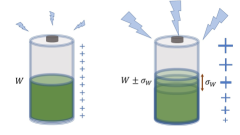
Figure 1: Fluctuations in extractable work limit the charging power of batteries. A quantum battery is a system that follows the laws of quantum physics, and that can store energy to be extracted later in order to perform work. The most important quantity in a battery is the maximum amount of work $W$ that can be extracted from it, i.e., the extractable work, which in certain cases is directly characterized by the free energy. However, due to the quantum nature of the battery, this free energy is a random quantity with uncertainties. We prove that the rate at which any battery can be charged is linked to such fluctuations, via fundamental bounds that hold for any charging protocol. For a battery with a well-defined value of the extractable work $W$, depicted on the left, the maximum rate at which the extractable work changes is zero. Fluctuations allow for faster charging rate, as illustrated on the right.

Isolated system analysis.— A protocol to extract work from a system and store it in a battery necessarily couples, at some point, the battery with the bath, the system, and/or auxiliary ancillas $\mathcal{A}$ used in order to implement the necessary operations. For instance, ancillas can be used to describe an arbitrary map acting on the system. We denote the system used as work reservoir, i.e. the battery, by $\mathcal{W}$, and its Hamiltonian by $H_{\mathcal{W}}$. We assume that the total system, consisting of all of the above, is isolated and evolves unitarily with a total Hamiltonian

$$H =H_{\mathcal{S}\mathcal{B}\mathcal{A}}\otimes\mathbbm{1}_{\mathcal{W}}+\mathbbm{1}_{\mathcal{S}\mathcal{B}\mathcal{A}}\otimes H_{\mathcal{W}}+V,$$ (2)

where $H_{\mathcal{S}\mathcal{B}\mathcal{A}}$ accounts for all terms that correspond to bath, system and ancilla evolution, $V$ incorporates all terms corresponding to interactions with the battery, and $\mathbbm{1}_{\{\cdot\}}$ denotes identities on the subspaces indicated by the subindex. Note that, while we allow $H_{\mathcal{S}\mathcal{B}\mathcal{A}}$ and $V$ to be explicitly time-dependent, we assume $H_{\mathcal{W}}$ to be time-independent, motivated by the idea of having a battery whose physical characteristics –e.g. Hamiltonian– do not change. Then, the full state $\rho$ of $\mathcal{S}\mathcal{B}\mathcal{A}\mathcal{W}$ evolves according to

$$\frac{d\rho}{dt}=-i[H,\rho].$$ (3)

For ease of notation we omit the explicit time-dependence of the evolving state $\rho$.

A central quantity behind the results of this Letter is the ‘free energy operator’, defined with respect to a bath at inverse temperature $\beta$ as

$$\mathcal{F}\equiv H_{\mathcal{W}}+\beta^{-1}\log\rho_{\mathcal{W}},$$ (4)

where $\rho_{\mathcal{W}}=\operatorname{\textnormal{Tr}}_{{\mathcal{S}\mathcal{B}\mathcal{A}}}\left({\rho}\right)$ is the state of the battery. The free energy operator $\mathcal{F}$ characterizes the amount of work that can be extracted from the battery, as from Eq. (1) it follows that

$$W_{\textnormal{max}}=\langle\mathcal{F}\rangle_{\mathcal{W}}-\langle\mathcal{F}\rangle_{\beta},$$ (5)

where $\langle\mathcal{F}\rangle_{\mathcal{W}}\equiv\operatorname{\textnormal{Tr}}\left({\mathcal{F}\rho_{\mathcal{W}}}\right)$ and $\langle\mathcal{F}\rangle_{\beta}\equiv\operatorname{\textnormal{Tr}}\left({\mathcal{F}\tau_{\beta}}\right)$. Note that, while $\mathcal{F}$ is a Hermitian operator, it depends on the state of the battery and it need not correspond to a physical observable. It is also worth stressing, though, that $\mathcal{F}$ is distinctively different to the process-dependent ‘work operator’ considered in Allahverdyan and Nieuwenhuizen (2005); Talkner et al. (2007); Perarnau-Llobet et al. (2017). Unlike the ‘work operator’, $\mathcal{F}$ corresponds to a state function, and its average characterizes the extractable work Brandão et al. (2013); Åberg (2014); Skrzypczyk et al. (2014b); Müller (2018b).

The rate at which the battery’s extractable work changes, that we refer to as the charging power, is given by

$$P(t) =\frac{dW_{\textnormal{max}}}{dt}=\frac{d\langle\mathcal{F}\rangle_{\mathcal{W}}}{dt}$$ (6)

$$=\frac{d\operatorname{\textnormal{Tr}}\left({\rho_{\mathcal{W}}H_{\mathcal{W}}}\right)}{dt}-\frac{1}{\beta}\frac{dS(\rho_{\mathcal{W}})}{dt},$$ (7)

where we used that $H_{\mathcal{W}}$ is time-independent. As proven in Rodríguez-Rosario et al. (2011); Das et al. (2018), it holds that $dS(\rho_{\mathcal{W}})/dt=-i\operatorname{\textnormal{Tr}}\left({V\left[\log\rho_{\mathcal{W}}\otimes\mathbbm{1}_{\mathcal{S}\mathcal{B}\mathcal{A}},\rho\right]}\right)$. Note that $P(t)$ limits the power needed in realistic charging protocols. Specifically, the energy $E$ needed to increase a battery’s extractable work by $\Delta W\equiv W_{\textnormal{max}}(t)-W_{\textnormal{max}}(0)$ in realistic charging protocols is bounded by the charging power, as $E\geq\Delta W=\int_{0}^{t}P(t^{\prime})dt^{\prime}$.

Using Eqs. (2) and (3), it further follows that $d\operatorname{\textnormal{Tr}}\left({\rho_{\mathcal{W}}H_{\mathcal{W}}}\right)/dt=-i\operatorname{\textnormal{Tr}}\left({[\rho,H_{\mathcal{W}}\otimes\mathbbm{1}_{\mathcal{S}\mathcal{B}\mathcal{A}}]V}\right)$. As a result,

$$P(t)= -i\operatorname{\textnormal{Tr}}\left({[\rho,H_{\mathcal{W}}\otimes\mathbbm{1}_{\mathcal{S}\mathcal{B}\mathcal{A}}]V}\right)$$

$$-i\frac{1}{\beta}\operatorname{\textnormal{Tr}}\left({\left[\rho,\log\rho_{\mathcal{W}}\otimes\mathbbm{1}_{\mathcal{S}\mathcal{B}\mathcal{A}}\right]V}\right)$$

$$= -i\operatorname{\textnormal{Tr}}\left({\left[\rho,\mathcal{F}\otimes\mathbbm{1}_{\mathcal{S}\mathcal{B}\mathcal{A}}\right]V}\right).$$ (8)

At a qualitative level, this simple derivation suggests that coherence in the eigenbasis of the free energy operator –which in turn necessitates coherence in the energy eigenbasis– serves to enhance the charging process. Indeed, if one considers a battery initially uncorrelated from other systems, $\rho=\rho_{\mathcal{W}}\otimes\rho_{\mathcal{S}\mathcal{B}\mathcal{A}}$, the charging power is zero unless the state is coherent in the eigenbasis of $\mathcal{F}$.

Our main result sets bounds on the charging power. Defining $\delta\mathcal{F}\equiv\mathcal{F}-\langle\mathcal{F}\rangle_{\mathcal{W}}$ and $\delta V=V-\langle V\rangle$, it holds that

$$P^{2}(t) \leq\Big{|}\operatorname{\textnormal{Tr}}\left({\rho\left[\delta\mathcal{F}\otimes\mathbbm{1}_{\mathcal{S}\mathcal{B}\mathcal{A}},\delta V\right]}\right)\Big{|}^{2}\leq 4\Big{|}\operatorname{\textnormal{Tr}}\left({\rho\,\delta\mathcal{F}\,\delta V}\right)\Big{|}^{2}$$

$$\leq 4\operatorname{\textnormal{Tr}}\left({\rho\left(\delta\mathcal{F}\right)^{2}\otimes\mathbbm{1}_{\mathcal{S}\mathcal{B}\mathcal{A}}}\right)\operatorname{\textnormal{Tr}}\left({\rho\left(\delta V\right)^{2}}\right),$$ (9)

where we use that $H_{\mathcal{W}}$ is time-independent and denote the averages of the extractable work and battery interaction energy by $\langle\mathcal{F}\rangle_{\mathcal{W}}=\operatorname{\textnormal{Tr}}\left({\rho_{\mathcal{W}}\mathcal{F}}\right)$ and $\langle V\rangle\equiv\operatorname{\textnormal{Tr}}\left({\rho V}\right)$, respectively. For the last step of the calculation we used the fact that for hermitian operators $A>0$, $B$ and $C$, the Cauchy-Schwarz inequality implies that $\text{Tr}^{2}\left(ABC\right)=\text{Tr}^{2}\left(\sqrt{A}BC\sqrt{A}\right)\leq\operatorname{\textnormal{Tr}}\left({AB^{2}}\right)\operatorname{\textnormal{Tr}}\left({AC^{2}}\right)$. Denoting the standard deviations of $\mathcal{F}$ and of the battery interaction Hamiltonian by $\sigma_{\mathcal{F}}$ and $\sigma_{V}$ respectively,

$$\sigma_{\mathcal{F}}^{2}(t) \equiv\left\langle\mathcal{F}^{2}\right\rangle_{\mathcal{W}}-\left\langle\mathcal{F}\right\rangle_{\mathcal{W}}^{2}$$ (10)

$$\sigma_{V}^{2}(t) \equiv\left\langle V^{2}\right\rangle-\left\langle V\right\rangle^{2},$$ (11)

Eq. (Fluctuations in extractable work bound the charging power of quantum batteries) implies

$$|P(t)|\leq 2\sigma_{\mathcal{F}}(t)\sigma_{V}(t).$$ (12)

This proves the existence of a trade-off between charging power and the fluctuations of the free energy operator $\mathcal{F}$: for a fixed interaction with the battery, a desired power input necessarily comes with fluctuations of the operator $\mathcal{F}$ whose mean characterizes the extractable work of the battery. In contrast, attempting to charge a battery with a deterministic amount of extractable work, such that $\sigma_{\mathcal{F}}=0$, leads to a null instantaneous charging power. It is straightforward to see that this implies, for instance, zero charging power for batteries in eigenstates of energy. We stress that this bound applies, in particular, to protocols that charge the battery via unitary evolution with a time-dependent perturbation Hamiltonian $V(t)$ Binder et al. (2015); Jaramillo et al. (2016); Campaioli et al. (2017); Ito and Miyadera (2017); Andolina et al. (2018); Julià-Farré et al. (2020a); Caravelli et al. (2020).

Open system analysis.— Evaluating bound (12) for charging protocols involving unitary, time-dependent, control of the battery is straightforward, as it solely involves knowledge of the state of the battery, its Hamiltonian $H_{\mathcal{W}}$, and the control Hamiltonian $V$. However, evaluating the factor $\sigma_{V}(t)$ may be hard for protocols that involve contact of the battery with secondary systems, as evaluating it requires specifying the full state $\rho$ of the battery and all the systems it interacts with. In the light of this, it is of practical importance to extend the analysis to encompass open-system descriptions of the dynamics of the battery, which we do next.

The formalism introduced so far allows to extend the analysis to include an open-system description of the dynamics of the battery. From Eq. (3), the state of the battery evolves according to

$$\frac{d}{dt}\rho_{\mathcal{W}} =-i\operatorname{\textnormal{Tr}}_{{\mathcal{S}\mathcal{B}\mathcal{A}}}\left({\left[H,\rho\right]}\right)$$

$$=-i[H_{\mathcal{W}},\rho_{\mathcal{W}}]-i\operatorname{\textnormal{Tr}}_{{\mathcal{S}\mathcal{B}\mathcal{A}}}\left({\left[V,\rho\right]}\right).$$ (13)

In the Markovian and weak-coupling limits the evolution of a system interacting with an environment is well approximated by

$$\frac{d}{dt}\rho_{\mathcal{W}} \approx-i[H_{\mathcal{W}},\rho_{\mathcal{W}}]-i[\tilde{H}_{\mathcal{W}},\rho_{\mathcal{W}}]$$ (14)

$$+\sum_{j}\gamma_{j}\left(L_{j}\rho_{\mathcal{W}}L_{j}^{\dagger}-\frac{1}{2}\left\{L_{j}^{\dagger}L_{j},\rho_{\mathcal{W}}\right\}\right),$$

where $\tilde{H}_{\mathcal{W}}$ accounts for the unitary part of the evolution due to the interactions, the Lindblad operators $L_{j}$ characterize the non-unitary effect of the interaction of the battery with the remaining systems, and the rates $\gamma_{j}$ are non-negative Breuer and Petruccione (2007). Then,

$$\operatorname{\textnormal{Tr}}_{{\mathcal{S}\mathcal{B}\mathcal{A}}}\left({\left[V,\rho\right]}\right)\approx[\tilde{H}_{\mathcal{W}},\rho_{\mathcal{W}}]$$ (15)

$$\quad\quad\quad+i\sum_{j}\gamma_{j}\left(L_{j}^{\dagger}\rho_{\mathcal{W}}L_{j}-\frac{1}{2}\left\{L_{j}^{\dagger}L_{j},\rho_{\mathcal{W}}\right\}\right).$$

With this, we prove in the Supplemental Material SM that the rate at which the extractable work of the battery changes is upper bounded by

$$|P(t)| \leq 2\sigma_{\mathcal{F}}(t)\sigma_{\tilde{H}_{\mathcal{W}}}(t)+\sum_{j}\gamma_{j}\sqrt{\left\langle\big{|}[\delta\mathcal{F},L_{j}]\big{|}^{2}\right\rangle}\|L_{j}\|,$$ (16)

where the operator norm $\|A\|$ is given by the largest modulus of the eigenvalues of an operator $A$, and $|A|^{2}=AA^{\dagger}$. This sets a bound valid for charging protocols based on open-system approaches. Importantly, the bound depends solely on the state $\rho_{\mathcal{W}}$ of the battery, and the decay rates $\gamma_{j}$ and operators $\widetilde{H}$ and $L_{j}$, fixed by the master equation that governs the dynamics of the battery.

Remarkably, for the open-system case it also holds that the charging power is null unless there exist fluctuations in the free energy operator $\mathcal{F}$. In order to see this, let $\ket{j}$ denote the eigenbasis of $\delta\mathcal{F}$, with $\delta\mathcal{F}=\sum_{j}w_{j}\ket{j}\bra{j}$, $\rho_{jk}=\bra{j}\rho_{\mathcal{W}}\ket{k}$ and $L_{jk}=\bra{j}L\ket{k}$. One then finds that

$$\left\langle\big{|}[\delta\mathcal{F},L_{j}]\big{|}^{2}\right\rangle=\sum_{jkl}\rho_{jk}L_{kl}L^{\dagger}_{lj}\left(w_{l}^{2}-w_{l}w_{j}-w_{l}w_{k}+w_{j}w_{k}\right).$$ (17)

As a result, for states $\rho_{\mathcal{W}}=\ket{j}\bra{j}$ with a deterministic amount of free energy characterized by $w_{j}$, one has that $\left\langle\big{|}[\delta\mathcal{F},L_{j}]\big{|}^{2}\right\rangle=0$ and that $\sigma_{\mathcal{F}}=0$, leading to a null charging rate $|P(t)|~{}=~{}0$. By contrast, states with support on more than one eigenstate of $\mathcal{F}$ can sustain a higher charging power, as both $\left\langle\big{|}[\delta\mathcal{F},L_{j}]\big{|}^{2}\right\rangle\neq 0$ and $\sigma_{\mathcal{F}}\neq 0$.

Finally, in the case of Hermitian Lindblad operators $L_{j}=L_{j}^{\dagger}$ we prove in the Supplemental Material SM that the bound (16) simplifies to

$$|P(t)| \leq\sigma_{\mathcal{F}}(t)\left(2\sigma_{\tilde{H}_{\mathcal{W}}}(t)+\sum_{j}2\gamma_{j}\|L_{j}\|^{2}\right).$$ (18)

Illustration with a heat engine.— We consider a minimal, self-contained, model of a heat engine that stores work in a quantum battery, as studied in detail in Linden et al. (2010); Brunner et al. (2012). The engine consists thermal baths at different temperatures, $T_{h}$ and $T_{c}$, as a resource. Note that these baths are internal to the workings of the protocol to extract energy; in particular, the temperatures $T_{h}$ and $T_{c}$ are unrelated to the inverse temperature $\beta$ of the reference bath with respect to which work is defined in Eq. (1).

In the engine, heat flow from the hot to the cold bath is exploited to extract work and store it in a toy-model battery that consists of a harmonic oscillator unbounded from below, with an energy gap $\epsilon$ for a Hamiltonian

$$H_{\mathcal{W}}=\sum_{n=-\infty}^{\infty}n\epsilon\ket{n}_{w}\!\bra{n}.$$ (19)

The storage device is indirectly coupled to the heat baths via a ‘switch’, consisting of two qubits. Qubit $1$, with energy gap $E_{1}$, is coupled to the cold bath, while qubit $2$, with energy gap $E_{2}$, is coupled to the hot bath. The qubits have a free Hamiltonian given by $H_{\mathcal{S}}=E_{1}\ket{1}_{1}\!\bra{1}+E_{2}\ket{1}_{2}\!\bra{1}$, with energies taken such that $E_{2}-E_{1}=\epsilon$, and they interact with the battery via

$$V=g\sum_{n}\Big{(}\ket{01,n}\!\bra{10,n+1}+\ket{10,n+1}\!\bra{01,n}\Big{)},$$ (20)

where $g$ is a coupling constant. Qubits $1$ and $2$ are assumed to thermalize due to the interaction with the thermal baths at rates $p_{1}$ and $p_{2}$, respectively. With these considerations, the evolution of the mean energy in the battery is solved analytically in Linden et al. (2010); Brunner et al. (2012), where it is found that choosing the parameters of the model correctly make the device work as a heat engine, storing work in $\mathcal{W}$.

We consider for simplicity a reference bath of zero temperature to calculate the extractable work of the battery. For this case, we derive the equations governing the dynamics of the charging power, extractable work, and its fluctuations in the Supplemental Material SM . We are interested in the charging power for initial states with uncertain amounts of free energy.

Consider first a state without uncertainty in the $\mathcal{F}$. For instance, consider qubits $1$ and $2$ initially in states $\tau_{1}$ and $\tau_{2}$ in thermal equilibrium with their respective thermal baths, and the battery in an eigenstate $\ket{0}_{\mathcal{W}}$ of its Hamiltonian,

$$\rho_{\textnormal{diag}} =\tau_{1}\otimes\tau_{2}\otimes\ket{0}_{\mathcal{W}}\bra{0}.$$ (21)

Naively, this would appear to be an ideal initial state for the battery, with a well-defined deterministic initial amount of energy and extractable work, without fluctuations. However, for such a state, diagonal in both interaction and battery Hamiltonians, Eq.  (8) implies that the engine initially functions with null power. This is illustrated in Fig. 2.

In order to have non-zero charging power for product states, a coherent superposition in the free energy operator and interaction Hamiltonian is needed. Consequently, we consider both the qubits and battery in a pure state, the latter in a superposition between $N$ energy levels $\ket{n}_{\mathcal{W}}$, with equal weights for simplicity:

$$\ket{\Psi_{N}} =\Big{(}\sqrt{r_{1}}\ket{0}_{1}+e^{i\theta}\sqrt{1-r_{1}}\ket{1}_{1}\Big{)}$$

$$\Big{(}\sqrt{r_{2}}\ket{0}_{2}+\sqrt{1-r_{2}}\ket{1}_{2}\Big{)}\frac{1}{\sqrt{N}}\sum_{n=0}^{N-1}\ket{n}_{\mathcal{W}}.$$ (22)

The phase $e^{i\theta}$ fixes whether the device works as an engine or a refrigerator.

With such coherent superposition as the initial state, one has $\sigma_{\mathcal{F}}\geq 0$ and $\sigma_{v}\geq 0$, such that inequality  (8) allows to have a non-zero charging power. This is to be compared with the null charging power of state $\rho_{\textnormal{diag}}$. Figure 2 compares the charging power $P(t)$ and the change in the extractable work $\Delta W\equiv W_{\textnormal{max}}(t)-W_{\textnormal{max}}(0)$ as a function of time, for initial states given by $\rho_{\textnormal{diag}}$ and $\ket{\Psi_{N}}\!\bra{\Psi_{N}}$, for different values of $N$. A superposition between eigenstates of $\mathcal{F}$ causes an increase in the charging power, with respect to the null charging power of the incoherent state. Superpositions between more levels results in an even higher power. This is reflected in the total extractable work as well, with a considerable increase for coherent superpositions, with the most noticeable advantage achieved when going from incoherent state to $\ket{\Psi_{2}}\!\bra{\Psi_{2}}$.

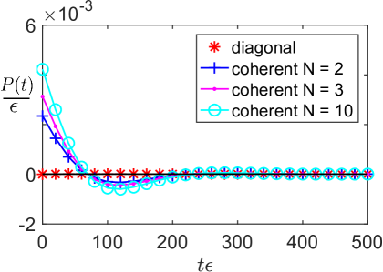
Figure 2: Charging power and extractable work. Charging power $P(t)$ (left) and change in extractable work $\Delta W\equiv W_{\textnormal{max}}(t)-W_{\textnormal{max}}(0)$ (right) as a function of time for various initial states (for the values of the parameters used see SM ). The incoherent state $\rho_{\textnormal{diag}}$ (red asterisk) has null charging power initially, as expected from bound (12). This charging power is slowly increased as the state supports higher fluctuations in extractable work. A significant increase in the charging power is seen for a coherent superposition of eigenstates of $\mathcal{F}$. For intermediate times this initial increase is penalized with a regime in which the battery is being discharged. Nevertheless, there is a net increase in the extractable work with respect to an incoherent initial state. Taking coherent superpositions between more than two states gives a further increase in charging power and extractable work.

Discussion.— We have established a direct relationship between the statistics of the extractable work and the charging power of batteries: for the latter to be non-zero the extractable work of the battery has to fluctuate. To this end, we have introduced bounds to the charging power in terms of a ‘free energy operator’ $\mathcal{F}~{}\equiv~{}H_{\mathcal{W}}+\beta^{-1}\log(\rho_{\mathcal{W}})$ whose expectation value equals the amount of maximum amount of work that can be extracted from the battery. Batteries in an eigenstate of $\mathcal{F}$ suffer from a null charging power, while fluctuations of $\mathcal{F}$ allow for higher charging rates. The bounds hold for a variety of battery charging protocols, including unitary dynamics of the battery via time-dependent perturbation Hamiltonians, isolated dynamics for battery-system-bath, as well as open-system dynamics. Our results also identify coherence as a resource in the process of work storage and should be of relevance to the engineering of quantum thermodynamic devices in a variety of platforms.

This work was funded by the John Templeton Foundation, UMass Boston Project No. P20150000029279, and DOE Grant No. DE-SC0019515. LPGP also acknowledges partial support by AFOSR MURI project “Scalable Certification of Quantum Computing Devices and Networks”, DoE ASCR FAR-QC (award No. DE-SC0020312), DoE BES Materials and Chemical Sciences Research for Quantum Information Science program (award No. DE-SC0019449), DoE ASCR Quantum Testbed Pathfinder program (award No. DE-SC0019040), NSF PFCQC program, AFOSR, ARO MURI, ARL CDQI, and NSF PFC at JQI.

García-Pintos et. al. Reply García-Pintos et al. (2021)

We acknowledge that a derivation reported in García-Pintos et al. (2020) is incorrect, as pointed out by Cusumano and Rudnicki Cusumano and Rudnicki (2021). We respond by giving a correct proof of the claim “fluctuations in the free energy operator upper bound the charging power of a quantum battery” that we made in the paper.

We thank Cusumano and Rudnicki for bringing to our attention the mistakes made in García-Pintos et al. (2020). Indeed, the conclusion that follows Eq. (17), and Eq. (18), are incorrect. As they have noted in Cusumano and Rudnicki (2021), without further conditions open quantum systems can have a non-zero charging power for batteries in an eigenstate of $\mathcal{F}$.

Even though expression (18) is incorrect, we stress that it holds that “fluctuations in the free energy operator bound the charging power of a quantum battery”, as claimed in the Letter. Equation (12) showed this for isolated quantum batteries, and this holds for open quantum batteries as well. We present a correct proof of this statement next.

The rate of change of the extractable work satisfies

$$P(t) =\frac{d\langle\mathcal{F}\rangle_{\mathcal{W}}}{dt}$$

$$=\frac{d}{dt}\operatorname{\textnormal{Tr}}\left({H_{\mathcal{W}}\rho_{\mathcal{W}}}\right)+\beta^{-1}\frac{d}{dt}\operatorname{\textnormal{Tr}}\left({\rho_{\mathcal{W}}\log(\rho_{\mathcal{W}})}\right)$$

$$=\operatorname{\textnormal{Tr}}\left({H_{\mathcal{W}}\frac{d\rho_{\mathcal{W}}}{dt}}\right)+\beta^{-1}\operatorname{\textnormal{Tr}}\left({\frac{d\rho_{\mathcal{W}}}{dt}\log(\rho_{\mathcal{W}})}\right)$$

$$=\operatorname{\textnormal{Tr}}\left({\frac{d\rho_{\mathcal{W}}}{dt}\mathcal{F}}\right),$$ (23)

where we used that the self-Hamiltonian $H_{\mathcal{W}}$ of the battery is time-independent García-Pintos et al. (2020) and that $\frac{d}{dt}\operatorname{\textnormal{Tr}}\left({\rho_{\mathcal{W}}\log(\rho_{\mathcal{W}})}\right)\nobreak=\nobreak\operatorname{\textnormal{Tr}}\left({\frac{d\rho_{\mathcal{W}}}{dt}\log(\rho_{\mathcal{W}})}\right)$ holds for finite dimensional systems as well as for states $\rho_{\mathcal{W}}$ with constant kernel Das et al. (2018).

Defining $\delta\mathcal{F}\nobreak\coloneqq\nobreak\mathcal{F}\nobreak-\nobreak\langle\mathcal{F}\rangle_{\mathcal{W}}$ and expressing the state of the battery in its instantaneous eigenbasis $\{\ket{\alpha}\}$ as $\rho_{\mathcal{W}}\nobreak=\nobreak\sum_{\alpha}p_{\alpha}\ket{\alpha}\!\bra{\alpha}$, the Cauchy-Schwarz inequality yields

$$\left|P(t)\right| =\left|\operatorname{\textnormal{Tr}}\left({\frac{d\rho_{\mathcal{W}}}{dt}\delta\mathcal{F}}\right)\right|=\bigg{|}\sum_{{\alpha\beta}}\delta\mathcal{F}_{\alpha\beta}\bra{\beta}\tfrac{d\rho_{\mathcal{W}}}{dt}\ket{\alpha}\bigg{|}$$

$$=\bigg{|}\sum_{\alpha\beta}\tfrac{\sqrt{p_{\alpha}+p_{\beta}}}{\sqrt{p_{\alpha}+p_{\beta}}}\delta\mathcal{F}_{\alpha\beta}\bra{\beta}\tfrac{d\rho_{\mathcal{W}}}{dt}\ket{\alpha}\bigg{|}$$

$$\leq\sqrt{\frac{1}{2}\sum_{\alpha\beta}(p_{\alpha}+p_{\beta})|\delta\mathcal{F}_{\alpha\beta}|^{2}}\sqrt{2\sum_{\alpha\beta}\tfrac{\left|\bra{\beta}\tfrac{d\rho_{\mathcal{W}}}{dt}\ket{\alpha}\right|^{2}}{p_{\alpha}+p_{\beta}}},$$ (24)

where we used that $\tfrac{d\rho_{\mathcal{W}}}{dt}$ is traceless and assumed differentiable dynamics.

The first factor in the bound is related to the fluctuations in the free energy operator, with $(\sigma_{\mathcal{F}})^{2}\nobreak=\nobreak\operatorname{\textnormal{Tr}}\left({\rho_{\mathcal{W}}(\delta\mathcal{F})^{2}}\right)\nobreak=\nobreak\sum_{\alpha\beta}p_{\alpha}|\delta\mathcal{F}_{\alpha\beta}|^{2}$. The second factor is related to the quantum Fisher information parametrized by time Helstrom (1969); Holevo (2011); Braunstein and Caves (1994),

$$\mathcal{I}_{F}\coloneqq 2\sum_{\alpha\beta}\frac{\left|\bra{\beta}\frac{d\rho_{\mathcal{W}}}{dt}\ket{\alpha}\right|^{2}}{p_{\alpha}+p_{\beta}},$$ (25)

which can diverge in instances of time when levels with $p_{\alpha}=0$ begin populating, but is otherwise finite for states with constant kernel. The Fisher information $\mathcal{I}_{F}$ characterizes the sensitivity of the state to time-translations, and determines the ultimate precision with which time can be estimated in the system (see Parisi (2009); Sidhu and Kok (2020) for accessible interpretations of the quantum Fisher information and its role in the study of quantum parameter estimation). The Fisher information has also been shown to bound the rate of change of the energy of quantum batteries Julià-Farré et al. (2020b), but note how the proof in Eq. (García-Pintos et. al. Reply García-Pintos et al. (2021)), in contrast, also incorporates the role of entropy to the extractable work.

We have thus proven that an interplay between the fluctuations in the free energy operator and the quantum Fisher information bound the rate of change of the extractable work,

$$\left|P(t)\right|\leq\sigma_{\mathcal{F}}\,\sqrt{\mathcal{I}_{F}}.$$ (26)

Given two states with identical Fisher information $\mathcal{I}_{F}$, the one with higher fluctuations in free energy can sustain a higher charging power.

Care needs to be taken for states whose rank is changing, since in those cases unpopulated states with $p_{\alpha}=0$ contribute to a divergent Fisher information. This is what happens for the initial state $\rho_{\mathcal{W}}(t_{0})=\ket{k_{0}}\!\bra{k_{0}}$ analyzed in García-Pintos et al. (2020) and by Cusumano and Rudnicki, since at $t_{0}$ a pure state is evolving to a mixed one. On the contrary, if at any $t\geq t_{0}$ the kernel of the state of the system is not changing, for instance for states with full support, Eq. (26) bounds power.

Appendix

.1 Limits to work extraction – open systems

The formalism introduced for isolated systems allows to extend the analysis to include an open-system description of the dynamics of the battery. Using that $d\rho/dt=-i[H,\rho]$, the state of the battery evolves according to

$$\frac{d}{dt}\rho_{\mathcal{W}} =-i\operatorname{\textnormal{Tr}}_{{\mathcal{S}\mathcal{B}\mathcal{A}}}\left({\left[H,\rho\right]}\right)$$

$$=-i\operatorname{\textnormal{Tr}}_{{\mathcal{S}\mathcal{B}\mathcal{A}}}\left({\left[\mathbbm{1}_{\mathcal{S}\mathcal{B}\mathcal{A}}\otimes H_{\mathcal{W}}+V,\rho\right]}\right)$$

$$=-i[H_{\mathcal{W}},\rho_{\mathcal{W}}]-i\operatorname{\textnormal{Tr}}_{{\mathcal{S}\mathcal{B}\mathcal{A}}}\left({\left[V,\rho\right]}\right).$$ (27)

In the Markovian limit the evolution is well approximated by

$$\frac{d}{dt}\rho_{\mathcal{W}} \approx-i[H_{\mathcal{W}},\rho_{\mathcal{W}}]-i[\tilde{H}_{\mathcal{W}},\rho_{\mathcal{W}}]$$ (28)

$$+\sum_{j}\gamma_{j}\left(L_{j}\rho_{\mathcal{W}}L_{j}^{\dagger}-\frac{1}{2}\left\{L_{j}^{\dagger}L_{j},\rho_{\mathcal{W}}\right\}\right),$$

where $\tilde{H}_{\mathcal{W}}$ accounts for the unitary part of the evolution due to the interactions, the Lindblad operators $L_{j}$ characterize the effect of the interaction of the battery with the remaining systems, and the rates $\gamma_{j}$ are non-negative Breuer and Petruccione (2007). Then,

$$\operatorname{\textnormal{Tr}}_{{\mathcal{S}\mathcal{B}\mathcal{A}}}\left({\left[V,\rho\right]}\right)\approx[\tilde{H}_{\mathcal{W}},\rho_{\mathcal{W}}]$$ (29)

$$\quad\quad\quad+i\sum_{j}\gamma_{j}\left(L_{j}\rho_{\mathcal{W}}L_{j}^{\dagger}-\frac{1}{2}\left\{L_{j}^{\dagger}L_{j},\rho_{\mathcal{W}}\right\}\right).$$

This allows to derive an alternative bound on the charging power that only depends on the state of the battery and the Lindblad operators. Defining $\delta\mathcal{F}\equiv\mathcal{F}-\langle\mathcal{F}\rangle_{\mathcal{W}}$, and using that

$$P_{t} =-i\operatorname{\textnormal{Tr}}\left({\rho\left[\mathcal{F}\otimes\mathbbm{1}_{\mathcal{S}\mathcal{B}\mathcal{A}},V\right]}\right),$$ (30)

it holds that

$$|P_{t}| =\Big{|}\operatorname{\textnormal{Tr}}\left({\rho[\mathcal{F}\otimes\mathbbm{1}_{\mathcal{S}\mathcal{B}\mathcal{A}},V]}\right)\Big{|}=\Big{|}\operatorname{\textnormal{Tr}}\left({\delta\mathcal{F}\otimes\mathbbm{1}_{\mathcal{S}\mathcal{B}\mathcal{A}}\left[V,\rho\right]}\right)\Big{|}$$

$$=\Big{|}\operatorname{\textnormal{Tr}}_{{\mathcal{W}}}\left({\delta\mathcal{F}\operatorname{\textnormal{Tr}}_{{\mathcal{S}\mathcal{B}\mathcal{A}}}\left({\left[V,\rho\right]}\right)}\right)\Big{|}$$

$$=\bigg{|}\operatorname{\textnormal{Tr}}_{{\mathcal{W}}}\left({\delta\mathcal{F}[\tilde{H}_{\mathcal{W}},\rho_{\mathcal{W}}]}\right)$$

$$\!\!\!\!\!\!\!+i\sum_{j}\gamma_{j}\operatorname{\textnormal{Tr}}_{{\mathcal{W}}}\left({\delta\mathcal{F}\left(L_{j}\rho_{\mathcal{W}}L_{j}^{\dagger}-\frac{1}{2}\left\{L_{j}^{\dagger}L_{j},\rho_{\mathcal{W}}\right\}\right)}\right)\bigg{|}$$

$$\leq\Big{|}\operatorname{\textnormal{Tr}}_{{\mathcal{W}}}\left({\delta\mathcal{F}[\tilde{H}_{\mathcal{W}},\rho_{\mathcal{W}}]}\right)\Big{|}$$

$$\!\!\!\!\!\!\!+\sum_{j}\gamma_{j}\left|\operatorname{\textnormal{Tr}}_{{\mathcal{W}}}\left({\delta\mathcal{F}\left(L_{j}\rho_{\mathcal{W}}L_{j}^{\dagger}-\frac{1}{2}\left\{L_{j}^{\dagger}L_{j},\rho_{\mathcal{W}}\right\}\right)}\right)\right|$$

$$=\Big{|}\operatorname{\textnormal{Tr}}_{{\mathcal{W}}}\left({\delta\mathcal{F}[\tilde{H}_{\mathcal{W}},\rho_{\mathcal{W}}]}\right)\Big{|}$$

$$\!\!\!\!\!\!\!+\sum_{j}\frac{\gamma_{j}}{2}\left|\operatorname{\textnormal{Tr}}_{{\mathcal{W}}}\left({[L_{j}^{\dagger},\delta\mathcal{F}]L_{j}\rho_{\mathcal{W}}+L_{j}^{\dagger}[\delta\mathcal{F},L_{j}]\rho_{\mathcal{W}}}\right)\right|$$ (31)

The Cauchy-Schwarz inequality implies that

$$\left|\operatorname{\textnormal{Tr}}_{{\mathcal{W}}}\left({L_{j}^{\dagger}[\delta\mathcal{F},L_{j}]\rho_{\mathcal{W}}}\right)\right|^{2}$$

$$\qquad\leq\operatorname{\textnormal{Tr}}_{{\mathcal{W}}}\left({\big{|}[\delta\mathcal{F},L_{j}]\big{|}^{2}\rho_{\mathcal{W}}}\right)\operatorname{\textnormal{Tr}}_{{\mathcal{W}}}\left({\big{|}L_{j}^{\dagger}\big{|}^{2}\rho_{\mathcal{W}}}\right)$$

$$\qquad\leq\operatorname{\textnormal{Tr}}_{{\mathcal{W}}}\left({\big{|}[\delta\mathcal{F},L_{j}]\big{|}^{2}\rho_{\mathcal{W}}}\right)\|L_{j}\|^{2}$$

$$\qquad\leq\left\langle\big{|}[\delta\mathcal{F},L_{j}]\big{|}^{2}\right\rangle\|L_{j}\|^{2},$$ (32)

and

$$\left|\operatorname{\textnormal{Tr}}_{{\mathcal{W}}}\left({\delta\mathcal{F}[\tilde{H}_{\mathcal{W}},\rho_{\mathcal{W}}]}\right)\right|^{2}\leq 4\sigma^{2}_{\mathcal{F}}(t)\sigma^{2}_{\tilde{H}_{\mathcal{W}}}(t).$$ (33)

Then,

$$|P_{t}| \leq 2\sigma_{\mathcal{F}}(t)\sigma_{\tilde{H}_{\mathcal{W}}}(t)+\sum_{j}\gamma_{j}\sqrt{\left\langle\big{|}[\delta\mathcal{F},L_{j}]\big{|}^{2}\right\rangle}\|L_{j}\|.$$ (34)

Interestingly, for the open-system case it also holds that the charging power is null unless there exist fluctuations in the extractable work of the battery. In order to see this, let $\delta\mathcal{F}=\sum_{j}w_{j}\ket{j}\bra{j}$. In the eigenbasis of $\delta\mathcal{F}$, one can write

$$\left\langle\big{|}[\delta\mathcal{F},L_{j}]\big{|}^{2}\right\rangle=\sum_{jkl}\rho_{jk}L_{kl}L^{\dagger}_{lj}\left(w_{l}^{2}-w_{l}w_{j}-w_{l}w_{k}+w_{j}w_{k}\right).$$ (35)

Thus, for states $\rho_{\mathcal{W}}=\ket{j}\bra{j}$ with a deterministic amount of free energy characterized by $w_{j}$, it follows that $\left\langle\big{|}[\delta\mathcal{F},L_{j}]\big{|}^{2}\right\rangle=0$ and that $\sigma_{\mathcal{F}}=0$, leading to

$$|P_{t}|=0.$$ (36)

In contrast, states with support on many eigenstates of $\mathcal{F}$ can sustain a higher charging power, as $\left\langle\big{|}[\delta\mathcal{F},L_{j}]\big{|}^{2}\right\rangle\neq 0$ and $\sigma_{\mathcal{F}}\neq 0$.

Note, too, that the third line of Eq. (.1) suggests that generating coherence in the eigenbasis of the free energy operator $\mathcal{F}$, or of the shifted Hamiltionian $\tilde{H}_{\mathcal{W}}$, may be beneficial for the charging power output.

Equation (34) can be further bounded for hermitian Lindblad operators, corresponding to pure dephasing. In that case, applying the Cauchy-Schwarz inequality, and using that $|\operatorname{\textnormal{Tr}}\left({ABC}\right)|=|\operatorname{\textnormal{Tr}}\left({ACB}\right)|$ for hermitian operators, gives

$$\left\langle\big{|}[\delta\mathcal{F},L_{j}]\big{|}^{2}\right\rangle \leq 4\|L_{j}\|^{2}\operatorname{\textnormal{Tr}}_{{\mathcal{W}}}\left({\rho_{\mathcal{W}}(\delta\mathcal{F})^{2}}\right)$$

$$=4\|L_{j}\|^{2}\sigma_{\mathcal{F}}^{2}(t).$$ (37)

That is, for hermitian Lindblad operators the charging rate is bounded by

$$|P_{t}| \leq\sigma_{\mathcal{F}}(t)\left(2\sigma_{\tilde{H}_{\mathcal{W}}}(t)+\sum_{j}2\gamma_{j}\|L_{j}\|^{2}\right).$$ (38)

.2 Bounds on charging rate – exact solution at zero temperature

For the case of a reference bath at zero temperature, the rate at which the extractable work –in this case energy– changes in the battery is

$$P(t)=\frac{d\operatorname{\textnormal{Tr}}\left({\rho_{\mathcal{W}}H_{\mathcal{W}}}\right)}{dt}.$$ (39)

Denoting the standard deviations of the extractable work and of the battery interaction Hamiltonian by $\sigma_{\mathcal{F}}$ and $\sigma_{V}$ respectively,

$$\sigma_{\mathcal{F}}^{2}(t) =\operatorname{\textnormal{Tr}}\left({\rho H_{\mathcal{W}}^{2}}\right)-\operatorname{\textnormal{Tr}}\left({\rho H_{\mathcal{W}}}\right)^{2}$$ (40)

$$\sigma_{V}^{2}(t) =\operatorname{\textnormal{Tr}}\left({\rho V^{2}}\right)-\operatorname{\textnormal{Tr}}\left({\rho V}\right)^{2},$$ (41)

the rate of extractable work with reference to a zero-temperature bath satisfies

$$\left|P(t)\right|\leq 2\sigma_{\mathcal{F}}(t)\sigma_{V}(t).$$ (42)

This implies a trade-off between extractable work (energy in this case) charging power and the fluctuations of the extractable work: for a fixed interaction with the battery, a desired power input necessarily comes with fluctuations in extractable work.

.2.1 Toy model of a heat engine

We illustrate the connection between charging power, fluctuations in the free energy operator $\mathcal{F}$, and quantum coherence, in a the simple toy model for a heat engine considered in Linden et al. (2010); Brunner et al. (2012). The engine, depicted in fig. 3, consists of a hot bath at temperature $T_{h}$ and a cold bath at temperature $T_{c}$ as resources.

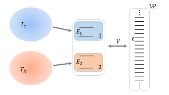
Figure 3: The heat engine stores work in the battery $\mathcal{W}$ by exploiting heat flowing from the hot to the cold baths. The baths and battery are coupled indirectly via qubits $1$ and $2$, working as a switch in the engine. As heat flows via the switch, the energy and extractable work stored in the battery increase.

Heat flow from the hot to the cold bath is exploited to extract work and store it in the battery, which consists of a Harmonic oscillator unbounded from below, with an energy gap $\epsilon$ in a Hamiltonian

$$H_{\mathcal{W}}=\sum_{n=-\infty}^{\infty}n\epsilon\ket{n}_{w}\!\bra{n}.$$ (43)

The storage device is indirectly coupled to the heat baths via a ‘switch’, consisting of two qubits. Qubit $1$, with energy gap $E_{1}$, is coupled to the cold bath, while qubit $2$, with energy gap $E_{2}$, is coupled to the hot bath. The qubits have a free Hamiltonian given by

$$H_{\mathcal{S}}=E_{1}\ket{1}_{1}\!\bra{1}+E_{2}\ket{1}_{2}\!\bra{1},$$ (44)

with energies taken such that $E_{2}-E_{1}=\epsilon$. The qubits interact with the battery via

$$V=g\sum_{n=-\infty}^{\infty}\Big{(}\ket{01,n}\!\bra{10,n+1}+\ket{10,n+1}\!\bra{01,n}\Big{)},$$ (45)

where $g$ is a coupling constant.

In the model, the qubits are assumed to thermalize due to the interaction with the thermal baths, which is modeled by the master equation

$$\frac{d\rho}{dt}=-i[H_{\mathcal{S}}+H_{\mathcal{W}}+V,\rho]+\sum_{i=1}^{2}p_{i}(\tau_{i}\operatorname{\textnormal{Tr}}_{{i}}\left({\rho}\right)-\rho),$$ (46)

where $\rho$ is the density matrix of the storage device and the qubits 1 and 2, and $p_{i}$ characterizes the rate at which qubit $`i^{\prime}$ thermalizes due to the interaction with its corresponding bath (see Linden et al. (2010); Brunner et al. (2012) for more details of the model). Thermal states of the qubits are denoted by

$$\tau_{i} =r_{i}\ket{0}_{i}\!\bra{0}+\overline{r_{i}}\ket{1}_{i}\!\bra{1},$$ (47)

with

$$\overline{r_{1}} =r_{1}e^{-\frac{E_{1}}{kT_{c}}},\qquad\overline{r_{2}}=r_{2}e^{-\frac{E_{2}}{kT_{h}}},$$ (48)

where $k$ is Boltzmann’s constant. If $E_{1}/T_{c}>E_{2}/T_{h}$ the device favors net energy exchange from hot to cold bath, working as a heat engine.

In Linden et al. (2010); Brunner et al. (2012) the authors show that the work deposited in the battery can be obtained from solving for $e_{\mathcal{W}}\equiv\operatorname{\textnormal{Tr}}\left({H_{\mathcal{W}}\rho_{\mathcal{W}}}\right)$,

$$\frac{de_{\mathcal{W}}}{dt}=\frac{d}{dt}\operatorname{\textnormal{Tr}}\left({H_{\mathcal{W}}\rho_{\mathcal{W}}}\right)=-ig\epsilon\Delta(t),$$ (49)

with

$$\Delta(t) =\sum_{n}\Big{(}\bra{01,n}\rho\ket{10,n+1}-\bra{10,n+1}\rho\ket{01,n}\Big{)}$$ (50a)

$$\Gamma_{1}(t) =\sum_{n}\Big{(}\bra{00,n}\rho\ket{00,n}+\bra{01,n}\rho\ket{01,n}\Big{)}$$ (50b)

$$\Gamma_{2}(t) =\sum_{n}\Big{(}\bra{00,n}\rho\ket{00,n}+\bra{10,n}\rho\ket{10,n}\Big{)},$$ (50c)

which obey the set of differential equations

$$\frac{d}{dt}\Delta(t) =2ig\Big{(}\Gamma_{1}(t)-\Gamma_{2}(t)\Big{)}-\big{(}p_{1}+p_{2}\big{)}\Delta(t)$$ (51a)

$$\frac{d}{dt}\Gamma_{1}(t) =ig\Delta(t)+p_{1}\Big{(}r_{1}-\Gamma_{1}(t)\Big{)}$$ (51b)

$$\frac{d}{dt}\Gamma_{2}(t) =-ig\Delta(t)+p_{2}\Big{(}r_{2}-\Gamma_{2}(t)\Big{)}.$$ (51c)

While Linden et al. (2010); Brunner et al. (2012) focuses on the general, asymptotic, behavior of the charging power, we are interested in the charging power when initial states with uncertain amounts of free energy, and quantum coherence, are taken. Consider first a state in which qubits $1$ and $2$ are initially in thermal equilibrium with their respective thermal baths, and the battery in an eigenstate of its Hamiltonian,

$$\rho_{\textnormal{diag}} =\Big{(}r_{1}\ket{0}_{1}\bra{0}+\overline{r_{1}}\ket{1}_{1}\bra{1}\Big{)}$$

$$\Big{(}r_{2}\ket{0}_{2}\bra{0}+\overline{r_{2}}\ket{2}_{1}\bra{2}\Big{)}\ket{0}_{\mathcal{W}}\bra{0}.$$ (52)

Naively, this sounds like an ideal initial state for the battery, with a well-defined deterministic initial amount of extractable work and energy, without fluctuations. However, for such a state, diagonal in both interaction and battery Hamiltonians, Eq. (8) in the main text implies that the engine initially functions with null power. Importantly, that the is the case for incoherent mixture states without deterministic initial free energy, e.g. thermal states.

In order to have non-zero charging power a coherent superposition in the battery and interaction Hamiltonians is needed (note, though, that this may not be sufficient). Consequently, we consider both the qubits and battery in a pure state, the latter in a superposition between $N$ energy levels, with equal weights for simplicity:

$$\ket{\Psi_{N}} =\Big{(}\sqrt{r_{1}}\ket{0}_{1}+e^{i\theta}\sqrt{\overline{r_{1}}}\ket{1}_{1}\Big{)}$$

$$\Big{(}\sqrt{r_{2}}\ket{0}_{2}+\sqrt{\overline{r_{2}}}\ket{1}_{2}\Big{)}\frac{1}{\sqrt{N}}\sum_{n=0}^{N-1}\ket{n}_{\mathcal{W}}.$$ (53)

The phase $e^{i\theta}$ can change the output of the engine, and even turn the device into a refrigerator during a transient time, for some values of $\theta$.

With such coherent superposition as the initial state one has $\sigma_{\mathcal{F}}\geq 0$ and $\sigma_{v}\geq 0$, such that inequality (8) in the main text allows to have a non-zero charging power. This is to be compared with the null charging power of state $\rho_{\textnormal{diag}}$. Figure 4 compares the charging power $P(t)$ and the change in the extractable work $\Delta W(t)\equiv W_{\textnormal{max}}(t)-W_{\textnormal{max}}(0)$ as a function of time, for initial states given by $\rho_{\textnormal{diag}}$ and $\ket{\Psi_{N}}\!\bra{\Psi_{N}}$, for different values of $N$. A superposition between two $H_{\mathcal{W}}$ eigenstates indeed causes an increase in the charging power, with respect to the null charging power of the incoherent state. Taking superpositions between more levels results in an even higher power. This is reflected in the total extractable work of battery as well, with a considerable increase for coherent superpositions, with the most noticeable advantage achieved when going from incoherent state to $\ket{\Psi_{2}}\!\bra{\Psi_{2}}$.

Charging power and extractable work

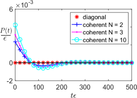
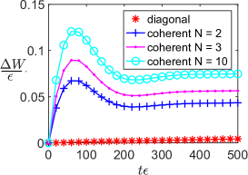
Figure 4: Charging power $P(t)$ (top) and change in extractable work $\Delta W(t)\equiv W_{\textnormal{max}}(t)-W_{\textnormal{max}}(0)$ (bottom) as a function of time for different initial states. The parameters in the model are takes as $p_{1}=p_{2}=g/\epsilon=0.01$, and $E_{1}/T_{c}=0.51$ and $E_{2}/T_{h}=0.50$. The phase in the initial states $\ket{\Psi_{N}}$ is taken $\theta=\pi/2$ to ensure a positive initial charging power (interestingly, for other phases the engine functions as a refrigerator). The incoherent state $\rho_{\textnormal{diag}}$ (red asterisk) has null charging power initially, as needs be from bound Eq. (12) in the main text. This charging power is slowly increased as the state supports higher fluctuations in the extractable work. A significant increase in the charging power is seen for a coherent superposition between 2 eigenvalues of $H_{\mathcal{W}}$. For intermediate times this initial increase is penalized with a regime in which the battery is being discharged though. Nevertheless, there is a significant net increase in the extractable work with respect to an incoherent initial state. Taking coherent superpositions between more than two states gives an even further increase in charging power and extractable work, but the increase is marginal for large superpositions, much smaller than the advantage of going from incoherent to minimal coherent superpositions.

While Fig. 4 illustrates the higher amount of extractable work obtained from states with coherence and non-zero extractable work fluctuations, it also raises the question of what happens with such fluctuations in extractable work. In order to study the evolution of the free energy variance, we consider

$$A(t)\equiv\operatorname{\textnormal{Tr}}\left({H_{\mathcal{W}}^{2}\rho_{\mathcal{W}}}\right).$$ (54)

Then

$$\sigma_{\mathcal{F}}^{2}(t)=A(t)-e_{\mathcal{W}}^{2}(t).$$ (55)

Similar calculations as in Linden et al. (2010); Brunner et al. (2012) show that

$$\frac{d}{dt}A(t)=-ig\epsilon^{2}\Delta(t)-2ig\epsilon^{2}\alpha(t),$$ (56)

where the system of differential equations is completed with

$$\frac{d}{dt}\alpha(t) =2ig\Big{(}\beta(t)-\gamma(t)-\delta(t)\Big{)}-(p_{1}+p_{2})\alpha(t)$$ (57a)

$$\frac{d}{dt}\beta(t) =ig\alpha(t)-p_{1}\beta(t)+\frac{p_{1}r_{1}}{\epsilon}e_{\mathcal{W}}(t)$$ (57b)

$$\frac{d}{dt}\gamma(t) =-ig\alpha(t)-p_{2}\gamma(t)+\frac{p_{2}r_{2}}{\epsilon}e_{\mathcal{W}}(t)-p_{2}r_{2}$$ (57c)

$$\frac{d}{dt}\delta(t) =p_{1}r_{1}\Gamma_{2}(t)+p_{2}r_{2}\Gamma_{1}(t)-(p_{1}+p_{2})\delta(t),$$ (57d)

and

$$\alpha(t) \equiv\sum_{n}n\Big{(}\bra{01,n}\rho\ket{10,n+1}-\bra{10,n+1}\rho\ket{01,n}\Big{)}$$ (58a)

$$\beta(t) \equiv\sum_{n}n\Big{(}\bra{00,n}\rho\ket{00,n}+\bra{01,n}\rho\ket{01,n}\Big{)}$$ (58b)

$$\gamma(t) \equiv\sum_{n}(n-1)\Big{(}\bra{00,n}\rho\ket{00,n}+\bra{10,n}\rho\ket{10,n}\Big{)}$$ (58c)

$$\delta(t) \equiv\sum_{n}\bra{00,n}\rho\ket{00,n}.$$ (58d)

Figure 5 depicts the fluctuations of the extractable work as a function of time for $\rho_{\textnormal{diag}}$ and $\ket{\Psi_{N}}\!\bra{\Psi_{N}}$ as initial states, for different values of $N$. As expected, coherent initial states, which have higher initial fluctuations, lead to final states with higher fluctuations than the diagonal state. However, the extractable work increases with coherent superpositions as well, resulting in an extractable work relative to the fluctuations that is considerably higher for coherent superpositions between few states ($N=2$ and $N=3$) than for the incoherent state. Further increasing the number of states in the superposition leads to a decrease in the extractable work relative to the fluctuations (although still higher than for $\rho_{\textnormal{diag}}$). Therefore, states in coherent superposition between few levels seem the most desirable: the extractable work greatly increases, while keeping relative fluctuations low.

This raises the discussion of the ‘quality’ of the extractable work. If one takes the average energy of the battery as the sole figure of merit for the work storage protocol, then considering states in coherent superpositions of energy eigenstates is better than diagonal states, resulting in higher charging power. On the other hand, for superpositions between many states the fluctuations of the extractable work increase considerably. On the other hand, when the fluctuations of the extractable work are taken into account, taking superpositions between few levels is better, resulting in an increase in the final amount of extractable work without considerably higher fluctuations than for a diagonal initial state.

Extractable work fluctuations and extractable work relative to fluctuations

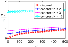
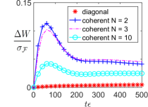
Figure 5: Extractable work fluctuations $\sigma_{\mathcal{F}}$ (left) and extractable work relative to the fluctuations $\Delta W/\sigma_{\mathcal{F}}$ (right) as a function of time for different initial states, with $p_{1}=p_{2}=g/\epsilon$, $E_{1}/T_{c}=0.51$, $E_{2}/T_{h}=0.50$, and $\theta=\pi/2$. The fluctuations in the extractable work for the incoherent state $\rho_{\textnormal{diag}}$ (red asterisk) are zero initially, but grow in time. For a coherent superposition between few (blue cross and purple dot) eigenvalues of $H_{\mathcal{W}}$ the initial fluctuations are significantly higher than for $\rho_{\textnormal{diag}}$, but the two become comparable for longer times. Since the engine produces a much higher extractable work output for the coherent state (see Fig. 4), the extractable work relative to the fluctuations is considerably higher for the coherent state. Taking coherent superpositions between many states (lightblue circle) gives a further increase the power fluctuations, which results in a lower extractable work relative to the fluctuations.

References

- Anders and Esposito (2017) J. Anders and M. Esposito, New Journal of Physics 19, 010201 (2017).
- Allahverdyan et al. (2004) A. E. Allahverdyan, R. Balian, and T. M. Nieuwenhuizen, Europhysics Letters (EPL) 67, 565 (2004).
- Brandão et al. (2013) F. G. S. L. Brandão, M. Horodecki, J. Oppenheim, J. M. Renes, and R. W. Spekkens, Phys. Rev. Lett. 111, 250404 (2013).
- Åberg (2014) J. Åberg, Phys. Rev. Lett. 113, 150402 (2014).
- Goold et al. (2016) J. Goold, M. Huber, A. Riera, L. del Rio, and P. Skrzypczyk, Journal of Physics A: Mathematical and Theoretical 49, 143001 (2016).
- (6) J. G. Richens and L. Masanes, Nature communications 7, 13511.
- Masanes and Oppenheim (2017) L. Masanes and J. Oppenheim, Nature communications 8, 14538 (2017).
- Alhambra et al. (2019) A. M. Alhambra, G. Styliaris, N. A. Rodríguez-Briones, J. Sikora, and E. Martín-Martínez, Phys. Rev. Lett. 123, 190601 (2019).
- Åberg (2013) J. Åberg, Nature communications 4, 1925 (2013).
- Frenzel et al. (2014) M. F. Frenzel, D. Jennings, and T. Rudolph, Phys. Rev. E 90, 052136 (2014).
- Jarzynski et al. (2015) C. Jarzynski, H. T. Quan, and S. Rahav, Phys. Rev. X 5, 031038 (2015).
- Alhambra et al. (2016) A. M. Alhambra, L. Masanes, J. Oppenheim, and C. Perry, Phys. Rev. X 6, 041017 (2016).
- Gallego et al. (2016) R. Gallego, J. Eisert, and H. Wilming, New Journal of Physics 18, 103017 (2016).
- Brandner et al. (2015) K. Brandner, M. Bauer, M. T. Schmid, and U. Seifert, New Journal of Physics 17, 065006 (2015).
- Lostaglio et al. (2015) M. Lostaglio, K. Korzekwa, D. Jennings, and T. Rudolph, Phys. Rev. X 5, 021001 (2015).
- Uzdin et al. (2015) R. Uzdin, A. Levy, and R. Kosloff, Phys. Rev. X 5, 031044 (2015).
- Korzekwa et al. (2016) K. Korzekwa, M. Lostaglio, J. Oppenheim, and D. Jennings, New Journal of Physics 18, 023045 (2016).
- Streltsov et al. (2017) A. Streltsov, G. Adesso, and M. B. Plenio, Reviews of Modern Physics 89, 041003 (2017).
- Francica et al. (2019) G. Francica, J. Goold, and F. Plastina, Phys. Rev. E 99, 042105 (2019).
- Latune et al. (2019) C. L. Latune, I. Sinayskiy, and F. Petruccione, Scientific Reports 9, 3191 (2019).
- Andolina et al. (2019a) G. M. Andolina, M. Keck, A. Mari, M. Campisi, V. Giovannetti, and M. Polini, Phys. Rev. Lett. 122, 047702 (2019a).
- Brunner et al. (2012) N. Brunner, N. Linden, S. Popescu, and P. Skrzypczyk, Phys. Rev. E 85, 051117 (2012).
- Linden et al. (2010) N. Linden, S. Popescu, and P. Skrzypczyk, Phys. Rev. Lett. 105, 130401 (2010).
- Correa et al. (2013) L. A. Correa, J. P. Palao, G. Adesso, and D. Alonso, Phys. Rev. E 87, 042131 (2013).
- Skrzypczyk et al. (2014a) P. Skrzypczyk, A. J. Short, and S. Popescu, Nature Communications 5, 4185 (2014a).
- Kosloff and Levy (2014) R. Kosloff and A. Levy, Annual Review of Physical Chemistry 65, 365 (2014).
- del Campo et al. (2014) A. del Campo, J. Goold, and M. Paternostro, Scientific reports 4 (2014), 10.1038/srep06208.
- Alicki and Gelbwaser-Klimovsky (2015) R. Alicki and D. Gelbwaser-Klimovsky, New Journal of Physics 17, 115012 (2015).
- Hofer et al. (2016) P. P. Hofer, M. Perarnau-Llobet, J. B. Brask, R. Silva, M. Huber, and N. Brunner, Phys. Rev. B 94, 235420 (2016).
- Niedenzu et al. (2016) W. Niedenzu, D. Gelbwaser-Klimovsky, A. G. Kofman, and G. Kurizki, New Journal of Physics 18, 083012 (2016).
- Caravelli et al. (2020) F. Caravelli, G. Coulter-De Wit, L. P. García-Pintos, and A. Hamma, Phys. Rev. Research 2, 023095 (2020).
- Funo and Ueda (2015) K. Funo and M. Ueda, Phys. Rev. Lett. 115, 260601 (2015).
- Funo et al. (2017) K. Funo, J.-N. Zhang, C. Chatou, K. Kim, M. Ueda, and A. del Campo, Phys. Rev. Lett. 118, 100602 (2017).
- Binder et al. (2015) F. C. Binder, S. Vinjanampathy, K. Modi, and J. Goold, New Journal of Physics 17, 075015 (2015).
- Jaramillo et al. (2016) J. Jaramillo, M. Beau, and A. del Campo, New Journal of Physics 18, 075019 (2016).
- Campaioli et al. (2017) F. Campaioli, F. A. Pollock, F. C. Binder, L. Céleri, J. Goold, S. Vinjanampathy, and K. Modi, Phys. Rev. Lett. 118, 150601 (2017).
- Ferraro et al. (2018) D. Ferraro, M. Campisi, G. M. Andolina, V. Pellegrini, and M. Polini, Phys. Rev. Lett. 120, 117702 (2018).
- Perarnau-Llobet and Uzdin (2019) M. Perarnau-Llobet and R. Uzdin, New Journal of Physics 21, 083023 (2019).
- Watanabe et al. (2017) G. Watanabe, B. P. Venkatesh, P. Talkner, and A. del Campo, Phys. Rev. Lett. 118, 050601 (2017).
- Watanabe et al. (2019) G. Watanabe, P. Venkatesh, B. P.and Talkner, M.-J. Hwang, and A. del Campo, arXiv e-prints , arXiv:1904.07811 (2019), arXiv:1904.07811 [quant-ph] .
- Müller (2018a) M. P. Müller, Phys. Rev. X 8, 041051 (2018a).
- Hovhannisyan et al. (2013) K. V. Hovhannisyan, M. Perarnau-Llobet, M. Huber, and A. Acín, Phys. Rev. Lett. 111, 240401 (2013).
- Friis and Huber (2018) N. Friis and M. Huber, Quantum 2, 61 (2018).
- Mandelstam and Tamm (1945) L. Mandelstam and I. Tamm, J. Phys.(USSR) 9, 1 (1945).
- Anandan and Aharonov (1990) J. Anandan and Y. Aharonov, Phys. Rev. Lett. 65, 1697 (1990).
- Margolus and Levitin (1998) N. Margolus and L. B. Levitin, Physica D: Nonlinear Phenomena 120, 188 (1998), proceedings of the Fourth Workshop on Physics and Consumption.
- Lloyd (2000) S. Lloyd, Nature 406, 1047 (2000).
- Lloyd (2002) S. Lloyd, Phys. Rev. Lett. 88, 237901 (2002).
- Giovannetti et al. (2003) V. Giovannetti, S. Lloyd, and L. Maccone, Phys. Rev. A 67, 052109 (2003).
- Taddei et al. (2013) M. M. Taddei, B. M. Escher, L. Davidovich, and R. L. de Matos Filho, Physical Review Letters 110, 050402 (2013).
- del Campo et al. (2013) A. del Campo, I. L. Egusquiza, M. B. Plenio, and S. F. Huelga, Physical Review Letters 110, 050403 (2013).
- Deffner and Lutz (2013) S. Deffner and E. Lutz, Physical Review Letters 111, 010402 (2013).
- Marvian et al. (2016) I. Marvian, R. W. Spekkens, and P. Zanardi, Phys. Rev. A 93, 052331 (2016).
- Shanahan et al. (2018) B. Shanahan, A. Chenu, N. Margolus, and A. del Campo, Phys. Rev. Lett. 120, 070401 (2018).
- Deffner and Campbell (2017) S. Deffner and S. Campbell, Journal of Physics A: Mathematical and Theoretical 50, 453001 (2017).
- An et al. (2016) S. An, D. Lv, A. del Campo, and K. Kim, Nature Communications 7, 12999 EP (2016).
- Campbell and Deffner (2017) S. Campbell and S. Deffner, Phys. Rev. Lett. 118, 100601 (2017).
- Ito and Miyadera (2017) K. Ito and T. Miyadera, ArXiv e-prints (2017), arXiv:1711.02322 [quant-ph] .
- Andolina et al. (2018) G. M. Andolina, D. Farina, A. Mari, V. Pellegrini, V. Giovannetti, and M. Polini, Phys. Rev. B 98, 205423 (2018).
- Julià-Farré et al. (2020a) S. Julià-Farré, T. Salamon, A. Riera, M. N. Bera, and M. Lewenstein, Phys. Rev. Research 2, 023113 (2020a).
- Andolina et al. (2019b) G. M. Andolina, M. Keck, A. Mari, V. Giovannetti, and M. Polini, Phys. Rev. B 99, 205437 (2019b).
- Skrzypczyk et al. (2014b) P. Skrzypczyk, A. J. Short, and S. Popescu, Nature Communications 5, 4185 (2014b).
- Müller (2018b) M. P. Müller, Phys. Rev. X 8, 041051 (2018b).
- Allahverdyan and Nieuwenhuizen (2005) A. E. Allahverdyan and T. M. Nieuwenhuizen, Phys. Rev. E 71, 066102 (2005).
- Talkner et al. (2007) P. Talkner, E. Lutz, and P. Hänggi, Phys. Rev. E 75, 050102 (2007).
- Perarnau-Llobet et al. (2017) M. Perarnau-Llobet, E. Bäumer, K. V. Hovhannisyan, M. Huber, and A. Acin, Phys. Rev. Lett. 118, 070601 (2017).
- Rodríguez-Rosario et al. (2011) C. A. Rodríguez-Rosario, G. Kimura, H. Imai, and A. Aspuru-Guzik, Phys. Rev. Lett. 106, 050403 (2011).
- Das et al. (2018) S. Das, S. Khatri, G. Siopsis, and M. M. Wilde, Journal of Mathematical Physics 59, 012205 (2018).
- Breuer and Petruccione (2007) H. P. Breuer and F. Petruccione, The Theory of Open Quantum Systems (Oxford University Press, New York, 2007).
- (70) See Supplemental Material for proof of bounds for open systems and details of the illustration on a model for a heat engine.
- Linden et al. (2010) N. Linden, S. Popescu, and P. Skrzypczyk, ArXiv e-prints (2010), arXiv:1010.6029 [quant-ph] .
- Brunner et al. (2012) N. Brunner, N. Linden, S. Popescu, and P. Skrzypczyk, Phys. Rev. E 85, 051117 (2012).
- García-Pintos et al. (2021) L. P. García-Pintos, A. Hamma, and A. del Campo, Phys. Rev. Lett. 127, 028902 (2021).
- García-Pintos et al. (2020) L. P. García-Pintos, A. Hamma, and A. del Campo, Phys. Rev. Lett. 125, 040601 (2020).
- Cusumano and Rudnicki (2021) S. Cusumano and L. Rudnicki, Phys. Rev. Lett. 127, 028901 (2021).
- Helstrom (1969) C. W. Helstrom, Quantum detection and estimation theory, Vol. 1 (Springer, 1969) pp. 231–252.
- Holevo (2011) A. S. Holevo, Probabilistic and statistical aspects of quantum theory, Vol. 1 (Springer Science & Business Media, 2011).
- Braunstein and Caves (1994) S. L. Braunstein and C. M. Caves, Phys. Rev. Lett. 72, 3439 (1994).
- Parisi (2009) M. G. Parisi, International Journal of Quantum Information 7, 125 (2009).
- Sidhu and Kok (2020) J. S. Sidhu and P. Kok, AVS Quantum Science 2, 014701 (2020).
- Julià-Farré et al. (2020b) S. Julià-Farré, T. Salamon, A. Riera, M. N. Bera, and M. Lewenstein, Phys. Rev. Research 2, 023113 (2020b).