Inference In High-dimensional Single-Index Models Under Symmetric Designs

Abstract

The problem of statistical inference for regression coefficients in a high-dimensional single-index model is considered. Under elliptical symmetry, the single index model can be reformulated as a proxy linear model whose regression parameter is identifiable. We construct estimates of the regression coefficients of interest that are similar to the debiased lasso estimates in the standard linear model and exhibit similar properties: $\sqrt{n}$-consistency and asymptotic normality. The procedure completely bypasses the estimation of the unknown link function, which can be extremely challenging depending on the underlying structure of the problem. Furthermore, under Gaussianity, we propose more efficient estimates of the coefficients by expanding the link function in the Hermite polynomial basis. Finally, we illustrate our approach via carefully designed simulation experiments.

Keywords: sparsity, debiased inference, compressed sensing, Hermite polynomials

1 Introduction and Background

The single-index model (SIM) has been the subject of extensive investigation in both the statistics and econometrics literatures over the last few decades. It generalizes the linear model to scenarios where the regression function $\mathbf{E}[y\mid x]$ is not necessarily linear in the covariates but depends on them through an unknown transformation of $\langle x,\tau\rangle$, where $\tau$ is the vector of regression co-efficients: $\mathbf{E}[y\mid x]=g(\langle x,\tau\rangle)$. While allowing broad generality in the structure of the mean response, the single-index model also circumvents the curse of dimensionality by modeling the mean response in terms of a low-dimensional functional of $x$. This precludes the need for fitting high-dimensional nonparametric models. An excellent review of single-index models appears, for example, in the work of Horowitz (2009).

It is well-known that the parameter $\tau$ is, in general, unidentifiable in the single-index model, since any scaling of $\tau$ can always be absorbed into the function $g$. Therefore, some identifiability constraints are imposed for statistical estimation and inference, a popular choice being to set $\|\tau\|=1$ and $\tau_{1}\geq 0$. General schemes for estimating $\tau$ involve optimizing an appropriate loss function (likelihood/pseudo-likelihood/least squares) in $(\underline{\tau},\underline{g})$ (generic parameter values) by alternately updating estimates of $\underline{\tau}$ and $\underline{g}$ (Carroll et al., 1997), or through a profile likelihood approach: see, e.g. the WNLS estimator in Section 2.5 of the work of Horowitz (2009). In any case, the estimation of $g$ figures critically in most estimation schemes. Inference on $\tau$ requires appropriate regularity assumptions on $g$, typically involving smoothness constraints, and while $g$ is only estimable at rate slower than $\sqrt{n}$, the parameter $\tau$ possesses $\sqrt{n}$-consistent asymptotically normal and efficient estimates, under certain regularity conditions.

High-dimensional single index models have also attracted interest with various authors studying variable selection, estimation and inference using penalization schemes. Ganti et al. (2015) use $\ell_{1}$ penalized estimates for learning high-dimensional index models were proposed and theoretical guarantees on excess risk for bounded responses was provided. Foster et al. (2013) proposed an algorithm for variable selection in a monotone single index model via the adaptive lasso. Luo and Ghosal (2016) proposed a penalized forward selection technique for high-dimensional single index models with a monotone link function. Cubic B-splines were employed by Cheng et al. (2017) for estimating the single index model in conjunction with a SICA (smooth integration of counting and absolute deviation) penalty function for variable selection. Radchenko (2015) studied simultaneous variable selection and estimation in high-dimensional SIMs using a penalized least-squares criterion, with the link function estimated via B-splines, and provided theoretical results on the rate of convergence. Yang et al. (2017) used a generalized version of Stein’s lemma that allows estimation of the regression vector under known but not necessarily Gaussian designs. Dudeja and Hsu (2018) and Pananjady and Foster (2019) consider estimation in single- and multi-index models by expanding the unknown link function in the Hermite polynomial basis. More recently, Hirshberg and Wager (2018) have proposed a method for average partial effect estimation in high-dimensional single-index models that is $\sqrt{n}$-consistent and asymptotically unbiased under sparsity assumptions on the regression coefficient, and to the best of our knowledge, this is the only work that provides asymptotic distributions in the high-dimensional setting. However, their method critically uses the form of the link function and also requires it to be adequately differentiable.

In this paper, we develop an inference scheme for the regression coefficients of a high-dimensional single-index model with minimal restrictions on the (potentially random) link function—indeed, even discontinuous link functions are allowed—that completely bypasses the estimation of the link. Thus, by dispensing with most regularity conditions on the link function, our approach can accommodate diverse underlying model structures. The price one pays for the feasibility of such an agnostic approach is an elliptically symmetric restriction on $X$. This assumption may be overly restrictive in applications where the entries of $X$ are determined by nature. However, in many applications one is allowed to design the measurement matrix. For example, in many applications of compressed sensing, Gaussian random matrices have been used as the measurement matrix, see for example the work of Candès and Wakin (2008) for an introduction to compressed sensing, the survey by Li et al. (2018) on one-bit compressed sensing and the work of Baraniuk and Steeghs (2007), Achim et al. (2014) for applications in radar and ultrasound imaging.

Next we introduce our model. Consider the semiparametric single-index model:

$$y_{i}=f_{i}(\langle x_{i},\tau\rangle),\quad i\in\{1,2,\dots,n\},$$ (1)

where $f_{i}:\mathbf{R}\rightarrow\mathbf{R}$ are iid realizations of an unknown random function $f$, independent of $x_{i}$, and $\tau\in\mathbf{R}^{p}$ is an unknown parameter whose direction is the object of estimation. Assume that $x_{i}\sim_{iid}N(0_{p},\Sigma)$ for a positive definite matrix $\Sigma$. While $\tau$ is not identifiable in this model, an appropriate scalar multiple: $\beta=\mu\tau$ (where $\mu$ will be defined shortly) is. As shown below, the new parameter $\beta$ turns out to be the vector of average partial derivatives of the regression function with respect to the covariates in the model, under certain conditions.

Notation. We will write $Y=(y_{1},\dots,y_{n})^{T}$, and let $X$ denote the matrix with $x_{1}^{T},\dots,x_{n}^{T}$ in its rows. For subsets of indices $I\subset\{1,\dots,n\},J\subset\{1,\dots,p\}$ we let $X_{I,J}$ be the submatrix of $X$ containing the rows with indices in $I$ and columns with indices in $J$. When $I$ or $J$ are singletons, we drop the brackets and identify $X_{I,k}$ with $X_{I,\{k\}}$ for $k=1,\dots,p$. Negative indices are used to exclude columns, so that for example $X_{i,-j}$ is the same as $X_{i,\{j\}^{c}}$. We denote by $\mathrm{e}_{j}$ the $j$-th element of the standard basis of $\mathbf{R}^{p}$. Finally, for two sequences $t_{n},s_{n}$ we write $t_{n}\lesssim s_{n}$ to mean $t_{n}\leq cs_{n}$ for $n\geq 1$ and a constant $c>0$ that does not depend on $n$.

For Gaussian covariates, there is a specific feature of this model that obviates the need to estimate the link function that we now describe. Throughout the paper we assume $\|\Sigma^{\frac{1}{2}}\tau\|_{2}=1$, as otherwise we can rescale $\tau$ and $f$ appropriately without changing $\beta$. Define:

$$\mu :=\mathbf{E}[y_{n}\langle x_{n},\tau\rangle]=\mathbf{E}[f(\zeta)\zeta],$$ (2)

$$\beta :=\mu\tau,$$ (3)

$$z :=Y-X\beta,$$ (4)

where $\zeta$ is a standard normal variable independent of $f$.

The parameter of interest $\beta$ can be viewed as an average partial effect. To see this, write $g(\langle x,\tau\rangle)=\mathbf{E}[y|X=x]$ and assume that $g$ is differentiable. The average partial effect with respect to the $j$-th covariate is then defined as:

$$\mathbf{E}_{x}\left[\frac{\partial}{\partial x_{j}}\mathbf{E}[y\mid x]\right] =\tau_{j}\mathbf{E}_{x}[g^{\prime}(\langle x,\tau\rangle)].$$

By Stein’s lemma (Stein, 1981), $\mathbf{E}[g^{\prime}(\langle x,\tau\rangle)]=\mathbf{E}\left[\langle x,\tau\rangle g(\langle x,\tau\rangle)\right]$, assuming both expectations exist and using the fact that $\langle x,\tau\rangle\sim N(0,1)$. Thus we have

$$\mathbf{E}_{x}\left[\frac{\partial}{\partial x_{j}}\mathbf{E}[y\mid x]\right] =\tau_{j}\mathbf{E}_{x}\left[\langle x,\tau\rangle\mathbf{E}[y\mid x]\right]=\tau_{j}\mathbf{E}[y\langle x,\tau\rangle]=\mu\tau_{j}=\beta_{j}.$$

As we seek to make inference on the importance/relative importance of the components of $\tau$ via estimates of $\beta$, we assume henceforth that $\mu\neq 0$. It can be shown (see C.1 in the appendix) that

$$\mathbf{E}[X^{T}z]=0,$$ (5)

which is equivalent to $\mathbf{E}[z_{i}x_{i}]=0$ for all $i=1,\dots,n$. We therefore have the representation $Y=X\beta+z$ with $X$ and $z$ uncorrelated, which implies that $\beta\in\arg\min_{\beta^{\prime}}\mathbf{E}\|Y-X\beta^{\prime}\|_{2}^{2}$, thus motivating the use of (penalized) least squares methods for estimation. The above equation will be referred to as the orthogonality property of $X$ and $z$ and will be used subsequently at several places.

The orthogonality property appears to have been first noted in the work of Brillinger (1982) who used it to study the properties of the least squares estimator $\hat{\beta}_{ls}$ in the classical fixed $p$ setting and showed that the estimator was asymptotically normal. Plan and Vershynin (2016) studied the estimation of $\beta$ in the $p>n$ setting using a generalized constrained lasso. While their results are quite general, they require knowing the constraint set $K$ over which least squares is performed. Under a different set of assumptions, Thrampoulidis et al. (2015) obtained an asymptotically exact expression for the estimation error of the regularized generalized lasso when $X$ has iid $N(0,1)$ entries and $\beta$ is generated according to a density in $\mathbf{R}^{p}$ with marginals that are independent of $p$.
Recall that a random vector $V$ is called spherically symmetric if its distribution is invariant to all possible rotations, i.e. $V\equiv_{d}PV$ for all orthogonal matrices $P$. Say that $X$ has an elliptically symmetric distribution if for some fixed vector $\mu$ and positive definite matrix $\Sigma$, $\Sigma^{-1/2}(X-\mu)$ is spherically symmetric. It turns out that the proxy linear model representation also holds more generally when $X$ follows an elliptically symmetric distribution since the proof of the orthogonality property (5) only uses the linearity of conditional expectations:

$$\mathbf{E}[x\mid\langle x,\tau\rangle]=\langle x,\tau\rangle b,$$

for a non-random vector $b\in\mathbf{R}^{p}$. The latter is a well-known property of elliptically symmetric distributions, see Appendix A for the details. This fact appears in the work of Li and Duan (1989), who then use the linear model representation to construct asymptotically normal and unbiased estimators of the regression coefficients in a fixed dimension parameter setting. More recently, Goldstein et al. (2018) have studied structured signal recovery (in high dimensions) from a single-index model with elliptically symmetric $X$, which can be viewed as an extension of Plan and Vershynin (2016).
Given the linear representation of the model as $Y=X\beta+z$, it is natural to ask the following questions:

• Can the debiasing techniques introduced in the setting of high-dimensional linear models be used for inference in single-index models?

• Can one improve on these procedures by going beyond a linear approximation?

Section 2 answers the first question in the affirmative by showing that under Gaussian design variants of the debiased Lasso estimator are consistent and asymptotically normally distributed. The second question is answered in Section 3 where, under Gaussian design, we improve the estimator in Section 2 by using an estimate of the link function in the debiasing procedure to improve the asymptotic variance. Our simulations show that this reduction in variance can be significant. Finally, in Appendix A we extend the aforementioned results to the case of elliptically symmetric designs with subgaussian tails.

2 Inference under Gaussian Design

In this section we apply the debiasing technique to obtain $\sqrt{n}$-consistent estimators of individual coordinates of $\beta$ under the assumption of Gaussian design. Our main theorems assume the existence of pilot estimators of $\beta$ that possess sufficiently fast ($\ell^{1}$-norm) rates of convergence. Subsection 2.4 discusses the construction of these pilot estimators. The extension of the results in this section to the case of elliptically symmetric design is considered in Appendix A.

2.1 Background on Debiased Lasso

The debiased lasso procedure proposed by Javanmard and Montanari (2014); Zhang and Zhang (2014); van de Geer et al. (2014) can be motivated as correcting the bias of low-dimensional projection estimators using the lasso estimate. More precisely, suppose that in a linear model $y=\langle x,\beta\rangle+\varepsilon$ the goal is to conduct inference on the first coordinate of $\beta$. In the low-dimensional scenario where $p<n$ and $\mathrm{rank}(X)=p$, the OLS estimate of $\beta_{1}$ can be written as

$$\hat{\beta}_{1}^{OLS}=\frac{u^{T}Y}{u^{T}X_{\cdot,1}},$$

where $u$ is the projection of the first column $X_{\cdot,1}$ on the orthocomplement of the span of $X_{\cdot,2},\dots,X_{\cdot,p}$. In the high-dimensional setting where $p>n$, this projection is typically zero, but one may still be able to find a vector $u$ for which $u^{T}X_{\cdot,1}$ is large while $\max_{j>1}|u^{T}X_{\cdot,j}|$ has a slow rate of growth. The bias of this projection estimator can further be reduced by using the Lasso estimate (Tibshirani, 1996) of $\beta$:

$$\tilde{\beta}_{1} :=\frac{u^{T}(Y-X_{\cdot,-1}\hat{\beta}_{-1}^{\text{lasso}})}{u^{T}X_{\cdot,1}}=\hat{\beta}_{1}^{\text{lasso}}+\frac{u^{T}(Y-X\hat{\beta}^{\text{lasso}})}{u^{T}X_{\cdot,1}},$$

$$\hat{\beta}^{\text{lasso}} :=\arg\min_{\beta^{\prime}}\left\{\frac{1}{2n}\|Y-X\beta^{\prime}\|_{2}^{2}+\lambda\|\beta^{\prime}\|_{1}\right\}.$$

A natural choice for the projection vector $u$ is $u=X\Sigma^{-1}\mathrm{e}_{1}$ when $\Sigma$ is known, used for example by Javanmard and Montanari (2018). Our estimator in Section 2.2 uses this choice up to a constant multiple. The analysis of this estimator is similar to the linear model setting and is included here as a stepping stone to the more involved analysis of later sections.
The estimator in Section 2.3 uses node-wise lasso to estimate (a multiple) of the first row of $\Sigma^{-1}$. The use of node-wise lasso was suggested previously by Zhang and Zhang (2014); van de Geer et al. (2014). Our estimator is slightly different in that we use sample splitting to break the dependence between the estimate of $\Sigma^{-1}$ and the approximation error $z$, whereas this is not necessary in linear models since the noise and the design are typically assumed to be independent.
Finally, in Section 3, we use a higher order expansion of the link function in the Hermite polynomial basis to further reduce the magnitude of the approximation error $z$ to obtain a more efficient estimator than the linear debiased estimator. Hermite polynomials provide a natural basis in our setting because of their orthogonality property under the Gaussian measure. Our estimator combines ideas from non-parametric and high-dimensional statistics and to the best of our knowledge has not been studied previously.

2.2 Inference on $\beta$ when $\Sigma$ is Known

We first consider the case where $\Sigma$ is known. In this case, the distribution of $x_{i}\sim N(0,\Sigma)$ is fully known, and we can therefore compute the $L_{2}$ projection of any covariate, $x_{n,1}$, over the remaining ones, $x_{n,-1}$. Specifically, define

$$\gamma:=\left(\mathbf{E}[x_{n,-1}x_{n,-1}^{T}]\right)^{-1}\mathbf{E}[x_{n,-1}x_{n,1}].$$

In words, $\gamma$ is the vector of coefficients when regressing the first covariate on the rest, at the population level. The resulting residuals $r_{i}:=x_{i,1}-\langle\gamma,x_{i,-1}\rangle$ satisfy

$$\mathbf{E}[r_{i}x_{i,-1}^{T}]=\mathbf{E}[x_{i,1}x_{i,-1}^{T}]-\gamma^{T}\mathbf{E}[x_{i,-1}x_{i,-1}^{T}]=0.$$

Suppose a sample size of size $2n$ is given. Then

• Compute the residuals $r_{i}$ as defined above on the first sub-sample $(x_{i},y_{i})_{i=1}^{n}$.

• Compute the lasso (Tibshirani, 1996) estimator $\hat{\beta}$ on the second subsample $(x_{i},y_{i})_{i=n+1}^{2n}$:

  $$\hat{\beta}\in\arg\min_{\beta^{\prime}}\left\{\frac{1}{2n}\sum_{i=n+1}^{2n}(y_{i}-\langle x_{i},\beta^{\prime}\rangle)^{2}+\lambda\|\beta^{\prime}\|_{1}\right\}$$

  with $\lambda\gtrsim\sigma_{x}\sigma_{z}\sqrt{\log(p)/n}$, where $\sigma_{x},\sigma_{z}$ are the subgaussian constants of $x_{n}$ and $z_{n}$, respectively.

Using these residuals and the pilot estimator $\hat{\beta}$, define a debiased estimator of $\beta_{1}$ as

$$\tilde{\beta}_{1}:=\hat{\beta}_{1}+\frac{\sum_{i=1}^{n}r_{i}(y_{i}-\langle x_{i},\hat{\beta}\rangle)}{\sum_{i=1}^{n}r_{i}x_{i,1}}.$$ (6)

The following theorem characterizes the asymptotic distribution of $\tilde{\beta}_{1}$.

Theorem 1

Suppose $(x_{i},y_{i})_{i=1}^{2n}$ follow model (1) with $x_{i}\sim N(0,\Sigma)$ and let

$$\nu^{2}=\frac{\mathbf{E}[r_{n}^{2}z_{n}^{2}]}{(\mathbf{E}[r_{n}^{2}])^{2}}.$$

Assume also that the following conditions are satisfied:

1. The sparsity of $\beta$ satisfies $s=o(\frac{n}{\log^{2}(p)})$.

2. There exist $0<c,C<\infty$ such that $c\leq\lambda_{\min}(\Sigma)\leq\lambda_{\max}(\Sigma)\leq C$.

3. $\mathbf{E}|y_{n}|^{2+\alpha}\leq M<\infty$ for some $\alpha,M>0$ and all $n\geq 1$.

4. The pilot estimator $\hat{\beta}$ satisfies

   $$\|\hat{\beta}-\beta\|_{2}\lesssim\sqrt{\frac{s\log(p)}{n}},\quad\text{ with probability }1-o(1).$$

Then

$$\sqrt{n}(\tilde{\beta}_{1}-\beta_{1})=\nu\cdot\Xi_{n},\quad\text{ where }\quad\Xi_{n}\rightarrow_{d}N(0,1).$$

Discussion of the Assumptions. The following points clarify the assumptions of the preceding theorem.

1. (Gaussianity / Elliptical Symmetry). Under the quadratic loss criterion, the population loss $\mathbf{E}[(y-\langle x,\beta^{\prime}\rangle)^{2}]$ is minimized at $\beta^{\star}=\beta+\Sigma^{-1}\mathbf{E}[(y-\langle x,\beta\rangle)x]$, where $\beta=\mu\tau$ is to be estimated. The bias term $\Sigma^{-1}\mathbf{E}[(y-\langle x,\beta\rangle)x]$ vanishes whenever

   $$\mathbf{E}[x\mid\langle x,\beta\rangle]=c\langle x,\beta\rangle$$ (7)

   for a fixed (non-random) vector $c\in\mathbf{R}^{p}$. This latter condition is satisfied for elliptically symmetric distributions and is the basis of the Lasso procedure used in our work. Details are provided in Appendix C.3. Section 6 in the work of Li and Duan (1989) analyzes estimation in low dimensional single-index models under departures from elliptical symmetry using arbitrary convex loss functions and establishes upper bounds on the bias of the corresponding M-estimators in terms of appropriate measures of such departures. The authors further consider the empirical counterparts of these measures as practical ways to verify the elliptical symmetry assumption. It is conceivable that similar diagnostic measures can work in our setting. For example, one can use sample splitting to estimate $\beta$ from a subsample and verify an empirical version of (7) on an independent subsample. These considerations are important for practice and can be the subject of future work. Another interesting extension would be to quantify the asymptotic distribution of the least squares estimator of $\beta$ in our setting under structured (as in adequately parametrized) violations of symmetry.

2. If the design matrix $X$ is not centered, but $\mathbf{E}[x_{n}]$ is known, then one can first center $X$ by using $\tilde{X}=X-\mathbf{E}X$ and redefining the link function:

   $$\tilde{f}_{i}(\cdot)=f_{i}(\cdot+\langle\mathbf{E}[x_{i}],\tau\rangle).$$

   Even though $f_{i}$ now depends on the mean of $x_{i}$, it is independent of $x_{i}$, and hence all the theoretical results in this paper continue to hold. In simulations we consider a case where $X$ has nonzero mean and is centered on the sample, prior to constructing the estimator (since, in reality, $\mathbf{E}[X]$ will not be known). While this, strictly speaking, does not fall within the purview of our approach (since the rows of $X-n^{-1}\mathbf{1}_{n}\mathbf{1}_{n}^{T}X$ are no longer independent), our inference procedure is still seen to produce satisfactory results in simulations.

3. Assumption 3 on the spectrum of $\Sigma$ is typically used in the high-dimensional inference literature, for example see the works of van de Geer et al. (2014); Javanmard and Montanari (2018, 2014). This assumption simplifies concentration arguments and also ensures that the design matrix satisfies the restricted eigenvalue condition with high probability.

Remark 2

1. In the special case of a standard linear model, i.e. when $y_{i}=\langle x_{i},\beta\rangle+\varepsilon_{i}$ with $\varepsilon_{i}\perp\!\!\!\!\perp x_{i}$, the asymptotic variance of $\sqrt{n}(\tilde{\beta}_{1}-\beta_{1})$ reduces to $\nu^{2}=\sigma^{2}/\mathbf{E}[r_{n}^{2}]$ which is the variance of the OLS estimator of $\beta_{1}$ in the low-dimensional case and the debiased estimator (van de Geer et al., 2014) in the high-dimensional case.

2. From the subgaussianity of $y_{n}$ and the Cauchy-Schwarz inequality, it follows that $\mathbf{E}[r_{n}^{2}z_{n}^{2}]$ is uniformly bounded above. Together with $\mathbf{E}[r_{n}^{2}]\geq\lambda_{\min}(\Sigma)$ (see Lemma 24 in the appendix for a proof of this), this shows that $\nu^{2}$ is uniformly bounded above and thus the rate of convergence of $\tilde{\beta}_{1}$ is indeed $\sqrt{n}$. On the other hand, if $\mathbf{E}[r_{n}^{2}z_{n}^{2}]=o(1)$, then the rate of convergence of $\tilde{\beta}_{1}$ is faster than $\sqrt{n}$, that is, we obtain $\sqrt{n}(\tilde{\beta}_{1}-\beta_{1})\rightarrow_{p}0$.

2.3 Inference when $\Sigma$ is Unknown

In this section we consider the problem of debiasing an estimate $\hat{\beta}_{1}$ of $\beta_{1}$ when the precision matrix $\Sigma^{-1}$ is unknown but estimable. Suppose that we have a sample $\mathcal{S}=(x_{i},y_{i})_{i=1}^{2n}$ of size $2n$, and that we use the second sub-sample $\mathcal{S}_{2}=(x_{i},y_{i})_{i=n+1}^{2n}$ to find an estimate $\hat{\gamma}$ of $\gamma$ using node-wise lasso (as proposed by van de Geer et al., 2014 in the setting of linear models):

$$\hat{\gamma}\in\arg\min_{\gamma^{\prime}}\left\{\frac{1}{2n}\sum_{i=n+1}^{2n}(X_{i,1}-\langle\gamma^{\prime},X_{i,-1}\rangle)^{2}+\lambda_{\text{node}}\|\gamma^{\prime}\|_{1}\right\}.$$ (8)

This estimate of $\gamma$ is then used to obtain estimates $\hat{r}_{i}$ of $r_{i}$ on the first sub-sample $\mathcal{S}_{1}=(x_{i},y_{i})_{i=1}^{n}$:

$$\hat{r}_{i}:=x_{i,1}-\langle x_{i,-1},\hat{\gamma}\rangle,\quad i\in\{1,\dots,n\}.$$ (9)

The debiased estimator of $\beta_{1}$ on the first subsample is then defined as

$$\tilde{\beta}_{1}:=\hat{\beta}_{1}+\frac{\sum_{i=1}^{n}\hat{r}_{i}(y_{i}-\langle x_{i},\hat{\beta}\rangle)}{\sum_{i=1}^{n}{\hat{r}_{i}x_{i,1}}},$$ (10)

where the pilot estimate $\hat{\beta}$ is is the lasso estimator:

$$\hat{\beta}\in\arg\min_{\beta^{\prime}}\left\{\frac{1}{2n}\sum_{i=1}^{n}(y_{i}-\langle x_{i},\beta^{\prime}\rangle)^{2}+\lambda_{\text{pilot}}\|\beta^{\prime}\|_{1}\right\}$$

with $\lambda_{\text{pilot}}\gtrsim\sigma_{x}\sigma_{z}\sqrt{\log(p)/n}$, and where $\sigma_{x},\sigma_{z}$ are the subgaussian constants of $x_{n}$ and $z_{n}$, respectively. The asymptotic distribution of the above estimator is characterized in the following theorem.

Theorem 3

Suppose $(x_{i},y_{i})_{i=1}^{2n}$ follow the model (1) with $x_{i}\sim N(0,\Sigma)$ and that the following conditions are satisfied:

1. We have $s:=\|\beta\|_{0}\lor\|\gamma\|_{0}=o(\frac{\sqrt{n}}{\log(p)})$.

2. The estimate $\hat{\gamma}$ of $\gamma$, depending on data in the second sub-sample $\mathcal{S}_{2}$, satisfies

   $$\mathbf{P}\left(\|\hat{\gamma}-\gamma\|_{1}\leq c_{\gamma}s\sqrt{\frac{\log p}{n}}\right)\rightarrow 1,$$

   for a constant $c_{\gamma}$ not dependent on $n$.

3. There exist $0<c,C<\infty$ such that $c\leq\lambda_{\min}(\Sigma)\leq\lambda_{\max}(\Sigma)\leq C$.

4. $z_{n}$ is subgaussian with $\|z_{n}\|_{\psi_{2}}\leq\sigma_{z}$ for some $\sigma_{z}<\infty$ not depending on $n$.

Then

$$\sqrt{n}(\tilde{\beta}_{1}-\beta_{1})=\nu\cdot\Xi_{n},\quad\text{ where }\quad\Xi_{n}\rightarrow N(0,1).$$

Discussion of assumptions. We provide a discussion of the assumptions of the theorem.

1. (Sufficient condition for assumption 4.) The approximation error $z_{n}=y_{n}-\langle x_{n},\beta\rangle$ is subgaussian whenever $y_{n}$ is subgaussian, since

   $$\|z_{i}\|_{\psi_{2}} \leq\|y_{n}\|_{\psi_{2}}+|\mu|\cdot\|\langle x_{i},\tau\rangle\|_{\psi_{2}},$$

   and $|\mu|$ is bounded by

   $$|\mu| =|\mathbf{E}[y_{n}\langle x_{n},\tau\rangle]|$$

   $$\leq\sqrt{\mathbf{E}[y_{n}^{2}]}\sqrt{\mathbf{E}[\langle x_{n},\tau\rangle^{2}]}$$

   $$\lesssim\|y_{n}\|_{\psi_{2}}.$$

   Thus $z_{n}$ is subgaussian and $\|z_{n}\|_{\psi_{2}}\lesssim\|y_{n}\|_{\psi_{2}}$. A similar argument shows the converse is also true and $\|y_{n}\|_{\psi_{2}}\leq\|z_{n}\|_{\psi_{2}}$.

2. Our approach to approximately de-correlating the design matrix uses sample splitting for estimation of $\gamma$, and the supporting argument is somewhat different from the ones in the work of Zhang and Zhang (2014), Javanmard and Montanari (2014) and van de Geer et al. (2014). This is because in our linear model $y_{i}=\langle x_{i},\beta\rangle+z_{i}$, the error $z_{i}$ is not independent of, but only uncorrelated with, $x_{i}$. Since our proof relies on the $\ell_{1}$ consistency of $\hat{\gamma}$, it necessitates sparsity of the rows of $\Sigma^{-1}$. It is not clear if the argument could be changed to justify the use of standard debiasing techniques (introduced in the aforementioned papers) that do not require sparsity assumptions on $\Sigma^{-1}$.

3. It is straightforward to see that given assumptions 1 and 3 of Theorem 3, assumption 2 is satisfied with high probability under a Gaussian design. First note that the eigenvalues of $\Sigma_{-1,-1}:=\mathbf{E}[x_{n,-1}x_{n,-1}^{T}]$ are within the interval $[\lambda_{\min}(\Sigma),\lambda_{\max}(\Sigma)]$ and hence by assumption 3 are bounded away from $0$ and $+\infty$. Using Lemma 23, this implies that the design matrix $X$ satisfies the restricted eigenvalue (RE) condition (with a restricted eigenvalue that is bounded away from zero) with probability $1-o(1)$ as $n\rightarrow\infty$. Next, by the definition of $\gamma$ and $r_{i}$ we can write

   $$x_{i,1}=\langle\gamma,x_{i,-1}\rangle+r_{i},\quad i=n+1,\dots,2n,$$

   where by construction $r_{i}$ and $x_{i,-1}$ are uncorrelated (and hence independent). Thus standard results for the lasso estimator (e.g. Theorem 7.2 of Bickel et al., 2009) guarantee with high probability that $\|\hat{\gamma}-\gamma\|_{1}\lesssim s\sqrt{\log(p)/n}$ as long as the tuning parameter satisfies $\lambda_{\text{node}}\gtrsim\lambda_{\max}(\Sigma)\sqrt{\log(p)/n}$. Obviously, all considerations here go through if instead of estimating $\beta_{1}$, we are interested in estimating $\beta_{k}$ for some other fixed $k$: we replace 1 by $k$ at the pertinent places.

Examples. In the following we provide examples that satisfy the assumptions of the above theorem.

• (Noisy one-bit compressed sensing). Suppose that $y=\operatorname{sign}(\langle x,\tau\rangle)\cdot\epsilon$ where $\tau$ is a s-sparse vector with $\|\tau\|_{2}=1$, $\epsilon\in\{1,-1\}$ is a random sign with $\mathbf{P}(\epsilon=1)=p\in[0,1]$ independent of $x\sim N(0,I)$. Variants of this model have been widely studied in the compressed sensing literature. See the survey by Li et al. (2018) for applications to wireless sensor networks, radar, and bio-signal processing. It is clear that assumptions 1 and 3 of Theorem 3 hold for this model. Note that in this model the rows of $\Sigma^{-1}=I$ are 1-sparse, and therefore the third remark above applies for the consistency of the node-wise lasso estimate $\hat{\gamma}$, implying the second assumption holds as well. To check the fourth assumption, use the boundedness of $y$ to write

  $$\|z\|_{\psi_{2}}\leq\|y\|_{\psi_{2}}+|\mu|\cdot\|\langle x,\tau\rangle\|_{\psi_{2}}\lesssim 1+|\mu|\leq 1+\sqrt{\frac{2}{\pi}}.$$

  The fifth assumption is also satisfied in light of Proposition 6.

• Suppose that $y=g(\langle x,\tau\rangle)+\varepsilon$ where $g$ is a fixed but unknown bounded or Lipschitz function, $x\sim N(0,\Sigma)$ with $\Sigma_{ij}=\rho^{|i-j|}$ for some fixed $\rho\in(0,1)$, and $\varepsilon$ is a mean-zero $\sigma$-subgaussian error independent of $x$. Then as long as $\|\tau\|_{0}=o(\sqrt{n}/\log(p))$, the assumptions of the theorem are satisfied. Note that in this case, $\Sigma$ is the correlation matrix of an $\mathrm{AR}(1)$ process, which is well-known to have a $2$-banded inverse covariance matrix. Therefore in this case $\|\gamma\|_{0}\leq 2$ and assumption 1 is satisfied. It can also be shown that $(1-\rho)/(1+\rho)\leq\lambda_{\min}(\Sigma)\leq\lambda_{\max}(\Sigma)\leq(1+\rho)/(1-\rho)$ (for example using Lemma 6 in the work of Gray (2006)), showing that assumption 3 is satisfied. The sub-gaussianity of $z=y-\langle\beta,x\rangle$ easily follows from the Lipschitz or boundedness assumption on the link function. For example, if $g$ is L-Lipschitz, then

  $$\|z\|_{\psi_{2}} \leq\|g(\langle x,\tau\rangle)\|_{\psi_{2}}+\|\mu\langle x,\tau\rangle\|_{\psi_{2}}+\sigma$$

  $$\leq\|L\cdot\langle x,\tau\rangle\|_{\psi_{2}}+\|\mu\langle x,\tau\rangle\|_{\psi_{2}}+\sigma$$

  $$\lesssim L+|\mu|+\sigma.$$

  Furthermore, $\mu$ is bounded by $L$ as well:

  $$|\mu| =\left|\mathbf{E}[g(\langle x,\tau\rangle)\langle x,\tau\rangle]\right|$$

  $$\leq\mathbf{E}[\left|g(\langle x,\tau\rangle)\right|\left|\langle x,\tau\rangle\right|]$$

  $$\leq L\mathbf{E}[\langle x,\tau\rangle^{2}]=L.$$

  Therefore as long as $\sigma$ and $L$ are uniformly bounded (in $n$), the subgaussian norm of $z$ is also uniformly bounded and assumption 4 is satisfied. The consistency of the lasso pilot estimator $\hat{\beta}$ and the node-wise estimate $\hat{\gamma}$ now follow from Proposition 6 and the third remark above.

Remark 4

In order to avoid loss of efficiency due to sample splitting, one can change the roles of the two sub-samples in the theorem to compute two estimates $\tilde{\beta}_{1}^{1},\tilde{\beta}_{1}^{2}$, and use the average of $\tilde{\beta}^{1}_{1}$ and $\tilde{\beta}^{2}_{1}$ as the final estimator. The proof of Theorem 3 shows that

$$\frac{\sqrt{n}(\tilde{\beta}_{1}^{m}-\beta_{1})}{\nu}=G^{m}+o_{p}(1),\quad m=1,2,$$

where

$$G^{m}=\frac{1}{\sqrt{n}}\frac{\sum_{i\in\mathcal{S}_{m}}r_{i}z_{i}}{\nu\mathbf{E}[r_{n}^{2}]}$$

depends only on the $m$-th subsample $\mathcal{S}_{m}$ so that $G^{1}$ and $G^{2}$ are independent. Moreover, we have $G^{m}\rightarrow_{d}N(0,1)$ as $n\rightarrow\infty$, and so by independence

$$G^{1}+G^{2}\rightarrow_{d}N(0,2).$$

Consequently, for the average estimator $\tilde{\beta}_{1}^{\text{avg}}=(\tilde{\beta}_{1}^{1}+\tilde{\beta}_{1}^{2})/2$ we have

$$\frac{\sqrt{2n}(\tilde{\beta}_{1}^{\text{avg}}-\beta_{1})}{\nu} =\frac{1}{\sqrt{2}}\left(\sqrt{n}\frac{(\tilde{\beta}_{1}^{1}-\beta_{1})}{\nu}+\sqrt{n}\frac{(\tilde{\beta}_{1}^{2}-\beta_{1})}{\nu}\right)$$

$$=\frac{1}{\sqrt{2}}(G^{1}+G^{2}+o_{p}(1))$$

$$\rightarrow_{d}N(0,1),$$

showing that the lost efficiency due to sample splitting is regained by switching the roles of sub-samples. This technique is well-known, see for example the work of Chernozhukov et al. (2018) for a similar application.

2.4 A Pilot Estimator of $\beta$

In this subsection the construction of a pilot estimator for $\beta$ is discussed. Consistency and rates of convergence of (generalized) constrained lasso estimators for single-index models under Gaussian or elliptically symmetric design have been established in other works, for example by Plan and Vershynin (2016) and Goldstein et al. (2018). In what follows we state and prove the consistency of penalized lasso under assumptions similar to the ones typically used in high dimensional linear models.

Let $\hat{\beta}$ be a solution to the penalized form of the lasso problem:

$$\hat{\beta}=\arg\min_{\beta^{\prime}}\left\{\frac{1}{2n}\|Y-X\beta^{\prime}\|_{2}^{2}+\lambda\|\beta^{\prime}\|_{1}\right\}.$$ (11)

In what follows we give sufficient conditions for consistency of $\hat{\beta}$, following the arguments in the work of Bickel et al. (2009). Before we state the proposition, we review the concept of restricted eigenvalues.

Definition 5 (Restricted eigenvalue condition)

A matrix $A$ is said to satisfy the restricted eigenvalue condition with parameters $(s,\kappa,\alpha)$, if for all $S\subset\{1,\dots,p\}$ with $|S|\leq s$ and all $\theta\in\mathbf{R}^{p}$ with $\|\theta_{S^{c}}\|_{1}\leq\kappa\|\theta_{S}\|_{1}$ we have $\|A\theta\|_{2}\geq\alpha\|\theta_{S}\|_{2}$. In this case we call $\alpha$ a restricted eigenvalue of $A$ (corresponding to parameters $(s,\kappa)$).

Proposition 6

Suppose that model (1) holds with $x\sim N(0,\Sigma)$ and let $\sigma_{x}^{2}=4\max_{j}\Sigma_{jj}$. Assume that

1. $z_{i}=y_{i}-\langle x_{i},\beta\rangle$ is subgaussian with $\|z_{i}\|_{\psi_{2}}\leq\sigma_{z}$,

2. $\beta$ is a $s$-sparse vector, i.e. $|\{j:\beta_{j}\neq 0\}|\leq s$,

3. $\Sigma^{\frac{1}{2}}$ satisfies the restricted eigenvalue condition with parameters $(s,9,2\alpha)$ for some $\alpha>0$, and that $\alpha$ and $\lambda_{\max}(\Sigma)$ are bounded away from $0,\infty$.

Then there exists an absolute constant $c_{0}>0$ such that for $\lambda>c_{0}\sigma_{z}\sigma_{x}\sqrt{\log(p)/n}$ and $n\geq c_{0}(1\lor\sigma_{x}^{4})s\log(p/s)$ we have

$$\|\hat{\beta}-\beta\|_{1} \leq\frac{12s\lambda}{\alpha^{2}},$$

$$\|\hat{\beta}-\beta\|_{2} \leq\frac{3\sqrt{s}\lambda}{\alpha^{2}},$$

$$\frac{\|X(\hat{\beta}-\beta)\|_{2}}{\sqrt{n}} \leq\frac{3\sqrt{s}\lambda}{\alpha},$$

with probability no less than $1-2p^{-1}-\exp(-c_{0}n^{2}/\sigma_{x}^{4})$.

Remark 7

Assumptions (2) and (3) in Proposition 6 are standard for the consistency of the lasso estimator, see the work of Bickel et al. (2009). Assumption (1) is the analogue of subgaussian errors in linear models and is satisfied whenever $y_{n}$ is subgaussian. This is a strong assumption on the approximation error $z_{i}$, but is nevertheless satisfied in several interesting cases such as when $y_{i}$ is bounded almost surely by a constant or when the model can be written as $y_{i}=g(\langle x_{i},\tau\rangle)+e_{i}$, where $g$ is an unknown Lipschitz function and $e_{i}$ is a mean-zero subgaussian error independent of $x_{i}$.

3 Towards More Efficient Inference

In previous sections, a linear approximation of the link function was used to obtain estimates of $\beta_{1}$. While this approach avoids the estimation of the link function, the (scaled) variance of the resulting estimator, $\nu^{2}=\mathbf{E}[r_{n}^{2}(y_{n}-\langle x_{n},\beta\rangle)^{2}]/(\mathbf{E}[r_{n}^{2}])^{2}$, depends heavily on the quality of this linear approximation.

Let us write $\mathbf{E}[y_{n}\mid x_{n}=x]=g(\langle x,\tau\rangle)$ and $e_{n}=y_{n}-g(\langle x_{n},\tau\rangle)$, so that $\mathbf{E}[e_{n}\mid x_{n}]=0$. In this section we show how, in the known $\Sigma$ regime and under smoothness assumptions on the link function $g$, we can go beyond a linear approximation and obtain more efficient estimators of $\beta_{1}$. To this end, we use an expansion of the link function in terms of Hermite polynomials, as the latter form an orthonormal basis of the Hilbert space $L^{2}(\mathbf{R},N(0,1))$ and are thus particularly useful in our setting.

The use of Hermite polynomials is readily motivated once we write $\langle x_{n},\beta\rangle=\mu\langle x_{n},\tau\rangle=\mu\cdot h_{1}(\langle x_{n},\tau\rangle)$, where $h_{1}(\xi)=\xi$ is the first-order Hermite polynomial, and $\mu$ is by definition

$$\mu=\mathbf{E}[y_{n}\langle x_{n},\tau\rangle]=\mathbf{E}[g(\xi)h_{1}(\xi)],\quad\xi\sim N(0,1).$$

Thus $\mu$ is the inner product of $g$ and $h_{1}$ in $L^{2}(\mathbf{R},N(0,1))$, and the debiasing procedure of Section 2 uses only the projection of the link function on $h_{1}$ to linearize the model.

Assume that $g$ can be expanded as $g(\xi)=\sum_{j=0}^{\infty}\mu_{j}h_{j}(\xi)$, where $h_{j}$ is the normalized Hermite polynomial of $j$-th degree:

$$h_{j}(\xi)=\frac{(-1)^{j}}{\sqrt{j!}}e^{\frac{\xi^{2}}{2}}\frac{d^{j}}{d\xi^{j}}e^{-\frac{\xi^{2}}{2}}.$$ (12)

The rest of this section considers an estimator of the form

$$\tilde{\beta}_{1}=\hat{\beta}_{1}+\frac{\sum_{i=1}^{n}r_{i}(y_{i}-\hat{g}_{m}(\langle x_{i},\hat{\tau}\rangle))}{\sum_{i=1}^{n}r_{i}x_{i1}},$$

where $\hat{g}_{m}=\sum_{j=0}^{m}\hat{\mu}_{j}h_{j}$ is a higher order estimate of $g$.

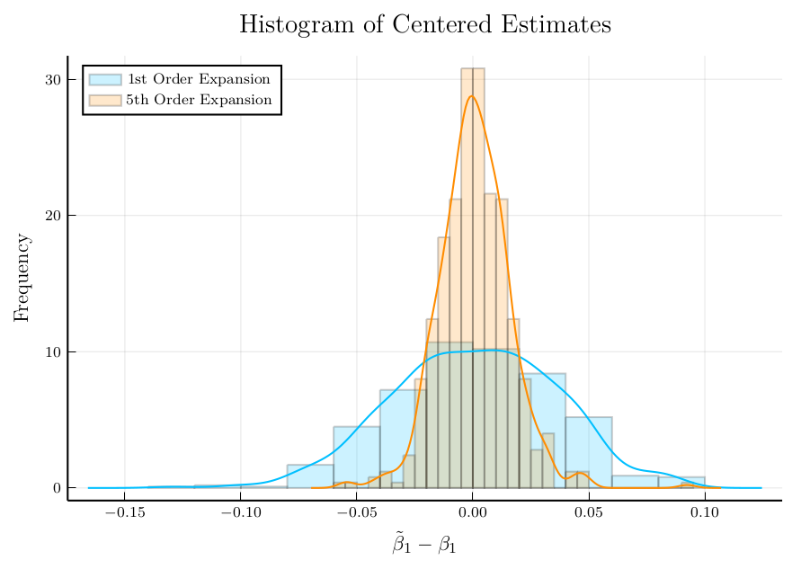
(a) Distribution of $\tilde{\beta}_{1}-\beta_{1}$

(b) A cubic link function and its estimate

Figure 1: Debiasing with Hermite polynomial expansions with link function $g(t)=5\sin(t)$. (a). The distribution of debiased estimator centered at $\beta_{1}$ is approximately Gaussian and centered at zero. The use of a 5th order expansion leads to significant improvement in variance. (b). The 5th order Hermite estimate of the link function (n = 2000, p = 3000).

In order to simplify notation, assume that we have a sample $(x_{i},y_{i})_{i=1}^{2n}$ of size $2n$. For a given $m$, we compute $\{\hat{\mu}_{j}\}_{j=1}^{m}$ and $\hat{\tau}$ on $\mathcal{S}_{2}=(x_{i},y_{i})_{i=n+1}^{2n}$ as in Algorithm 1:

Data: An iid sample $(x_{i},y_{i})_{i=1}^{2n}$

Input: Tuning parameters $m,\lambda_{\text{pilot}},$

1. Set $\hat{\beta}:=\arg\min_{\beta^{\prime}}\left\{\lfloor n/2\rfloor^{-1}\sum_{i=n+1}^{n+\lfloor n/2\rfloor}(y_{i}-\langle x_{i},\beta^{\prime}\rangle)^{2}+\lambda_{\text{pilot}}\|\beta^{\prime}\|_{1}\right\}$.

2. Define $\hat{\mu}_{1}:=\|\Sigma^{\frac{1}{2}}\hat{\beta}\|_{2}$ and $\hat{\tau}:=\hat{\mu}_{1}^{-1}\hat{\beta}$.

3. For $0\leq j\leq m$ and $j\neq 1$ set $\hat{\mu}_{j}:=\frac{1}{\lceil n/2\rceil}\sum_{i=n+\lfloor n/2\rfloor+1}^{2n}y_{i}h_{j}(\langle x_{i},\hat{\tau}\rangle)$.

4. return

   $$\tilde{\beta}_{1}:=\hat{\beta}_{1}+\frac{\sum_{i=1}^{n}r_{i}(y_{i}-\sum_{j=0}^{m}\hat{\mu}_{j}h_{j}(\langle x_{i},\hat{\tau}\rangle))}{\sum_{i=1}^{n}r_{i}x_{i1}}\,.$$ (13)

Algorithm 1 Hermite Estimator with Known $\Sigma$

Theorem 8

Suppose that $(x_{i},y_{i})_{i=1}^{2n}$ are i.i.d. observations from the model

$$y_{i}=g(\langle\tau,x_{i}\rangle)+e_{i},\quad x_{i}\sim N_{p}(0,\Sigma),\quad\mathbf{E}[e_{i}|x_{i}]=0.$$

Let $m=\lfloor\log^{\frac{2}{3}}(n)\rfloor$ and suppose that $\hat{\beta},\hat{\tau},\{\hat{\mu}_{j}\}_{j=0}^{m}$ are computed as in Algorithm 1. Assume also that the following conditions are satisfied:

1. There exist $0<c,C<\infty$ such that $c\leq\lambda_{\min}(\Sigma)\leq\lambda_{\max}(\Sigma)\leq C$.

2. There exists a constant $c^{\prime}>0$ such that $|\mu_{1}|=|\mathbf{E}[y_{n}\langle x_{n},\tau\rangle]|>c^{\prime}$ for all $n\geq 1$.

3. The response $y_{n}$ has a finite fourth moment: $\mathbf{E}[y_{n}^{4}]<C_{y}^{4}$.

4. The link function $g$ is differentiable with

   $$\|g^{\prime}\|_{L_{2}}^{2}=\underset{\xi\sim N(0,1)}{\mathbf{E}}|g^{\prime}(\xi)|^{2}<L^{2}<\infty,$$

   for a constant $L$ not depending on $n$.

5. The sparsity of $\beta$ satisfies $s=o(\frac{n}{\log^{2}(p)})$.

6. $\mathbf{E}|e_{n}|^{2+\alpha}<M<\infty$ for some $\alpha,M>0$ and all $n\geq 1$.

7. The pilot estimator $\hat{\beta}$ satisfies

   $$\|\hat{\beta}-\beta\|_{2}\lesssim\sqrt{\frac{s\log(p)}{n}}\quad\text{ with probability }1-o(1).$$

Then

$$\sqrt{n}(\tilde{\beta}_{1}-\beta_{1})=\nu\cdot\Xi_{n},\quad\text{ where }\Xi_{n}\rightarrow_{d}N(0,1),\text{ and }\nu^{2}=\frac{\mathbf{E}[r_{n}^{2}e_{n}^{2}]}{(\mathbf{E}[r_{n}^{2}])^{2}}.$$

Remark 9

1. Inspecting the proof of Theorem 8 shows that the argument in remark (4) applies here as well, so that changing the role of the two subsamples $\mathcal{S}_{1}$ and $\mathcal{S}_{2}$ leads to efficient use of the full sample.
2. Our second assumption requiring that $|\mu_{1}|$ be bounded away from zero ensures that $\hat{\tau}:=\hat{\mu}_{1}^{-1}\hat{\beta}$ enjoys similar consistency properties as $\hat{\beta}$. Even though our proof breaks down if $\mu_{1}=o(1)$, other pilot estimates of $\hat{\tau}$ exist that do not require a non-vanishing $\mu_{1}$. An interesting example is the work of Dudeja and Hsu (2018) proposing to estimate $\tau$ by maximizing $\hat{F}_{l}(\tau^{\prime})=n^{-1}\sum_{1}^{n}y_{i}h_{l}(\langle\tau^{\prime},x_{i}\rangle)$ over the unit sphere for an appropriately chosen $l\in\{1,2,\dots\}$. The consistency of this estimator instead requires $\mu_{l}\neq 0$ since $\mathbf{E}[\hat{F}_{l}(\tau^{\prime})]=\mu_{l}\langle\tau,\tau^{\prime}\rangle^{l}$ when $\Sigma=I$ (see the identity (14) below for inner products of Hermite polynomials).

Remark 10 (Efficiency)

1. Using $y_{n}=g(\langle x_{n},\tau\rangle)+e_{n}$ and $\mathbf{E}[e_{n}|x_{n}]=0$ we can write

$$\mathbf{E}[r_{n}^{2}z_{n}^{2}]=\mathbf{E}[r_{n}^{2}(y_{n}-\langle x_{n},\beta\rangle)^{2}]=\mathbf{E}[r_{n}^{2}(g(\langle x_{n},\tau\rangle)-\langle x_{n},\beta\rangle)^{2}]+\mathbf{E}[r_{n}^{2}e_{n}^{2}]\geq\mathbf{E}[r_{n}^{2}e_{n}^{2}],$$

with equality happening if and only if $\mathbf{E}[r_{n}^{2}(g(\langle x_{n},\tau\rangle)-\langle x_{n},\beta\rangle)^{2}]=0$. This shows that the estimator in Theorem 8 is strictly more efficient than the one in Theorem 1, unless $g(\langle x_{n},\tau\rangle)=\mu\cdot\langle x_{n},\tau\rangle$ almost everywhere, in which case the asymptotic variances are equal.

2. (Lower bound on variance reduction). Let $\tilde{\beta}_{1}^{L}$ denote the debiased estimate obtained by linearization (as in Theorem 1) and $\tilde{\beta}_{1}^{H}$ be the estimate from Hermite expansion. Also assume that $g,g^{\prime},g^{\prime\prime}\in L^{2}(N(0,1))$. The reduction in asymptotic variance (scaled by $n$) is given by

$$n(\mathbf{Var}[\tilde{\beta}_{1}^{L}]-\mathbf{Var}[\tilde{\beta}_{1}^{H}])\approx\sum_{\stackrel{{\scriptstyle j=0}}{{j\neq 1}}}^{\infty}\left[\frac{\mu_{j}^{2}}{\mathbf{E}[r_{n}^{2}]}+2\tau_{1}^{2}\left(j\mu_{j}^{2}+\sqrt{(j+1)(j+2)}\mu_{j}\mu_{j+2}\right)\right].$$

A proof is given in Proposition 31 in the appendix. To gain some intuition, consider the special case where $\Sigma=I$ so that $\|\tau\|_{2}=\mathbf{E}[r_{n}^{2}]=1$. Then simple algebra after using the inequality $2\sqrt{(j+1)(j+2)}\mu_{j}\mu_{j+2}\geq-(j+1)\mu_{j}^{2}-(j+2)\mu_{j+2}^{2}$ shows that the right-hand side of the above display is lower bounded by

$$(1-\tau_{1}^{2})\sum_{j=0,j\neq 1}^{\infty}\mu_{j}^{2}=(1-\tau_{1}^{2})\mathbf{E}[(g(\langle x,\tau\rangle)-\langle x,\beta\rangle)^{2}].$$

The growth rate of $m$. In Theorem 8 we let the number of basis functions $\{h_{j}\}_{j=0}^{m}$ grow with $n$ at the rate $m=\lfloor\log^{\frac{2}{3}}(n)\rfloor$. The theorem continues to remain valid for slower rates of growth of $m$, as long as $m\rightarrow\infty$. The slow growth rate of $m$ is used to bound the variance of $\hat{\mu}_{j}$ via the fourth moment of $h_{j}(\langle\tau,x\rangle)$ which is exponential in $j$ (see Proposition 25). While this rate of growth guarantees improvement in the $n\rightarrow\infty$ asymptotic regime, providing lower/upper bounds on the MSE in terms of $m$ for a fixed sample size $n$ is more challenging as these bounds would depend on the Hermite coefficients of the particular link function. To see this, observe that in Figure 2, the MSE (and similarly, the variance) initially oscillates on odd/even ordered Hermite expansions. In the particular case of $g(t)=5\sin(t)$ this can be explained by the fact that $\sin(t)$ is an odd function, so the even ordered Hermite coefficients are all zero. Thus adding even-ordered terms, for a fixed sample size, only adds noise without explaining any of the variance.
For implementation in practice, one can use a jackknife estimate of the variance to find the $m$ that minimizes the variance for a given sample size $n$. Note that, since the bias is typically negligible compared to the standard error (see Tables 1 and 2), the Mean Squared Error (MSE) is largely determined by the variance so that minimizing the variance will also minimize the MSE. Figure 2 shows agreement between the optimal $m$ for the MSE and its jackknife based estimate.

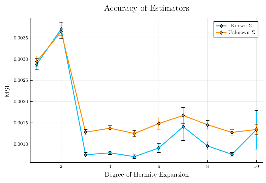
(a) Mean Squared Error of Debiased Estimates

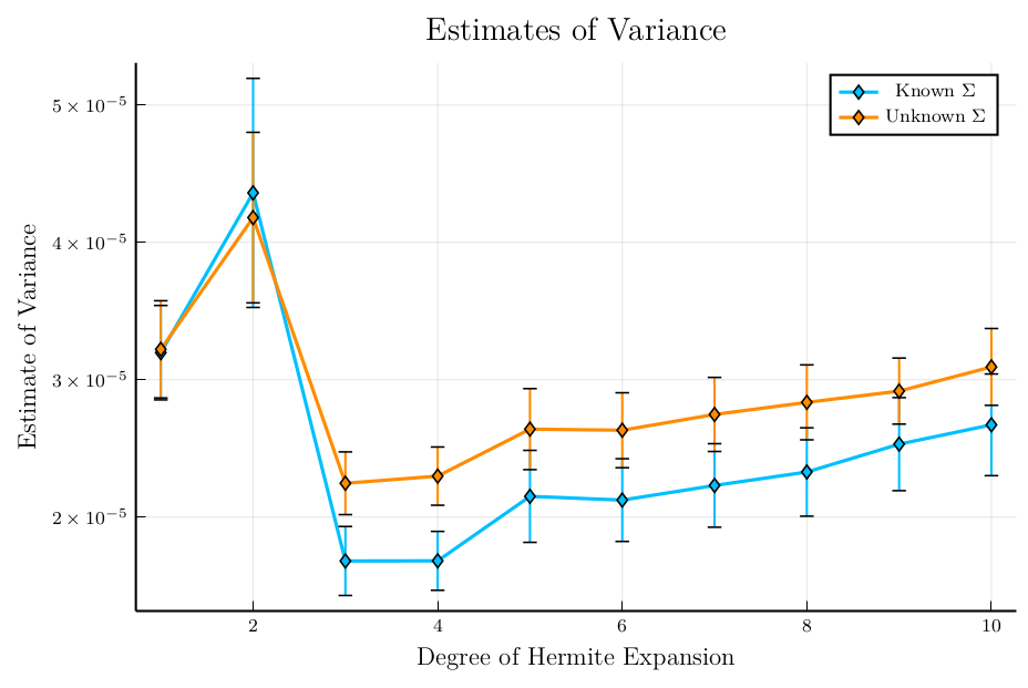
(b) Jackknife Estimates of Standard Error

Figure 2: (a). The effect of higher order expansions on the Mean Squared Error (MSE). For each degree of expansion, the empirical MSEs were computed based on 1000 replications and are shown by the solid lines while the respective error bars denote their empirical standard errors. (b). The Jackknife (leave-$k$-out) estimates of variance (up to a factor that does not depend on $m$) can be used to tune the order $m$ of the Hermite expansion. In this case, the solid lines depict the mean (computed over 10 realizations) of the jackknife estimate of the variance of the debiased estimator, and the error bars as before reflect the standard error of this quantity.

3.1 Inference when $\Sigma$ is unknown

The estimator proposed in the previous section uses $\Sigma$ and $\gamma$ in the definition of $\hat{\mu}_{1}$ and $r_{i}$ respectively. When $\Sigma$ is unknown, it is natural to instead set $\hat{\mu}_{1}:=\|\hat{\Sigma}^{\frac{1}{2}}\hat{\beta}\|_{2}$. Similarly, one can define $r_{i}=x_{i,1}-\langle\hat{\gamma},x_{i,-1}\rangle$ where $\hat{\gamma}$ is obtained using node-wise lasso as described in Section 2.2.

The main difficulty in the case of unknown $\Sigma$ is that it is not possible to exactly standardize $\langle\hat{\tau},x\rangle$ to have a $N(0,1)$ distribution. This is important in our analysis of the bias and variance of the estimator because the Hermite polynomials are only orthogonal with respect to standard normal random variables. More specifically, in the case of known $\Sigma$ we heavily use the following identity of O’Donnell (2014) which is only valid for unit vectors $\alpha,\hat{\alpha}\in\mathbf{R}^{p}$:

$$\mathbf{E}[h_{j}(\langle\alpha,x\rangle)h_{k}(\langle\hat{\alpha},x\rangle)]=\langle\alpha,\hat{\alpha}\rangle^{j}\mathbf{1}[j=k],\quad\text{ for }x\sim N_{p}(0,I).$$ (14)

Our Proposition 28 in the appendix generalizes this identity to non-unit vectors $\alpha,\hat{\alpha}$ as follows

$$\mathbf{E}[h_{j}(\langle\alpha,x\rangle)h_{k}(\langle\hat{\alpha},x\rangle)]=\sqrt{j!k!}\sum_{\stackrel{{\scriptstyle 0\leq i\leq\min\{j,k\}}}{{j\equiv_{2}i\equiv_{2}k}}}\frac{\langle\alpha,\hat{\alpha}\rangle^{i}\left(\frac{\|\alpha\|_{2}^{2}-1}{2}\right)^{\frac{j-i}{2}}\left(\frac{\|\hat{\alpha}\|_{2}^{2}-1}{2}\right)^{\frac{k-i}{2}}}{i!(\frac{j-i}{2})!(\frac{k-i}{2})!},$$

where $x\sim N_{p}(0,I)$ and $i\equiv_{2}j$ means that $i-j$ is an even integer. As suggested by the above display, using $\hat{\Sigma}$ to studentize $\langle\hat{\tau},x\rangle$ leads to non-orthogonality of the Hermite polynomials, which in turn introduces extra bias terms in the error decomposition of the debiased estimator. In order to control these extra errors a slower rate of growth of $m=\lfloor\log^{\frac{1}{4}}(n)\rfloor$ (compared with $m=\lfloor\log^{\frac{2}{3}}(n)\rfloor$ in Theorem 8) is assumed in Theorem 11.

Data: An iid sample $(x_{i},y_{i})_{i=1}^{2n}$

Input: Tuning parameters $m,\lambda_{\text{pilot}},\lambda_{\text{node}}$

1. Set $\check{\beta}:=\arg\min_{\beta^{\prime}}\left\{(2n)^{-1}\sum_{i=1}^{n}(y_{i}-\langle x_{i},\beta^{\prime}\rangle)^{2}+\lambda_{\text{pilot}}^{\prime}\|\beta^{\prime}\|_{1}\right\}$

2. Set $\hat{\beta}:=\arg\min_{\beta^{\prime}}\left\{(2\lfloor n/3\rfloor)^{-1}\sum_{i=n+1}^{n+\lfloor n/3\rfloor}(y_{i}-\langle x_{i},\beta^{\prime}\rangle)^{2}+\lambda_{\text{pilot}}\|\beta^{\prime}\|_{1}\right\}$.

3. Set $\hat{\gamma}:=\arg\min_{\gamma^{\prime}}\left\{\lfloor n/3\rfloor^{-1}\sum_{i=n+\lfloor n/3\rfloor+1}^{n+2\lfloor n/3\rfloor}(x_{i1}-\langle x_{i,-1},\gamma^{\prime}\rangle)^{2}+\lambda_{\text{node}}\|\gamma^{\prime}\|_{1}\right\}$.

4. Set $\hat{\Sigma}:=\lfloor n/3\rfloor^{-1}\sum_{i=n+\lfloor n/3\rfloor+1}^{n+2\lfloor n/3\rfloor}x_{i}x_{i}^{T}$.

5. Set $\hat{\mu}_{1}:=\|\hat{\Sigma}^{\frac{1}{2}}\hat{\beta}\|_{2}$ and $\hat{\tau}:=\hat{\mu}_{1}^{-1}\hat{\beta}$.

6. For $0\leq j\leq m$ and $j\neq 1$ set $\hat{\mu}_{j}:=\sum_{i=n+2\lfloor n/3\rfloor+1}^{2n}y_{i}h_{j}(\langle x_{i},\hat{\tau}\rangle)/(n-2\lfloor n/3\rfloor)$.

7. return $\tilde{\beta}_{1}:=\check{\beta}_{1}+\frac{\sum_{i=1}^{n}\hat{r}_{i}(y_{i}-\langle\check{\beta}-\hat{\beta},x_{i}\rangle-\sum_{j=0}^{m}\hat{\mu}_{j}h_{j}(\langle x_{i},\hat{\tau}\rangle))}{\sum_{i=1}^{n}\hat{r}_{i}x_{i1}}\,$.

Algorithm 2 Hermite Estimator with Unknown $\Sigma$

Theorem 11

Suppose that $(x_{i},y_{i})_{i=1}^{2n}$ are i.i.d. observations from the model

$$y_{i}=g(\langle\tau,x_{i}\rangle)+e_{i},\quad x_{i}\sim N_{p}(0,\Sigma),\quad\mathbf{E}[e_{i}|x_{i}]=0.$$

Let $m=\lfloor\log^{\frac{1}{4}}(n)\rfloor$ and suppose that $\hat{\beta},\hat{\tau},\{\hat{\mu}_{j}\}_{j=0}^{m}$ are computed as in Algorithm 2. Assume also that the following conditions are satisfied:

1. There exist $0<c,C<\infty$ such that $c\leq\lambda_{\min}(\Sigma)\leq\lambda_{\max}(\Sigma)\leq C$.

2. There exists a constant $c^{\prime}>0$ such that $|\mu_{1}|=|\mathbf{E}[y_{n}\langle x_{n},\tau\rangle]|>c^{\prime}$ for all $n\geq 1$.

3. The link function $g$ is differentiable with

   $$\|g^{\prime}\|_{L_{2}}^{2}=\underset{\xi\sim N(0,1)}{\mathbf{E}}|g^{\prime}(\xi)|^{2}<L^{2}<\infty,$$

   for a constant $L$ not depending on $n$.

4. We have $s:=\|\beta\|_{0}\lor\|\gamma\|_{0}=o(\frac{\sqrt{n}}{\log(p)})$.

5. The estimate $\hat{\gamma}$ of $\gamma$, satisfies

   $$\mathbf{P}\left(\|\hat{\gamma}-\gamma\|_{1}\leq c_{\gamma}s\sqrt{\frac{\log p}{n}}\right)\rightarrow 1,\text{ and }\,\mathbf{P}\left(\|\hat{\gamma}-\gamma\|_{2}\leq c_{\gamma}^{\prime}\sqrt{\frac{s\log p}{n}}\right)\rightarrow 1,$$

   for constants $c_{\gamma},c_{\gamma}^{\prime}$ not dependent on $n$.

6. $\mathbf{E}|e_{n}|^{2+\alpha}<M<\infty$ for some $\alpha,M>0$ and all $n\geq 1$.

7. $z_{n}$ is subgaussian with $\|z_{n}\|_{\psi_{2}}\leq\sigma_{z}$ for some $\sigma_{z}<\infty$ and all $n\geq 1$.

Then

$$\sqrt{n}(\tilde{\beta}_{1}-\beta_{1})=\nu\cdot\Xi_{n}+o_{p}(1),\quad\text{ where }\Xi_{n}\rightarrow_{d}N(0,1),\text{ and }\nu^{2}=\frac{\mathbf{E}[r_{n}^{2}e_{n}^{2}]}{(\mathbf{E}[r_{n}^{2}])^{2}}+\frac{\mu_{3}^{2}\tau_{1}^{2}}{(\mathbf{E}[r_{n}^{2}])^{2}}.$$

Remark 12

The variance of the $\tilde{\beta}_{1}$ in Theorem 11 has an extra term $\frac{\mu_{3}^{2}\tau_{1}^{2}}{(\mathbf{E}[r_{n}^{2}])^{2}}$ compared with the case of known $\Sigma$. The inflated variance is due to the error in estimation of $\Sigma$ by $\hat{\Sigma}$. Since by assumption $\mathbf{E}[r_{n}^{2}]\geq\lambda_{\min}(\Sigma)$ is bounded away from zero, we obtain the same variance as in Theorem 8 if $\mu_{3}\tau_{1}=o(1)$.

3.2 Simulations

Next we describe our setup for the simulations. We consider the effect of up to the tenth order Hermite expansions on the bias and variance of the debiased estimator. We take the nonlinear link function to be:

$$g(t)=5\sin(t),$$

and define $\tau$ by

$$\tau=\frac{\iota}{\sqrt{\iota^{T}\Sigma\iota}}\text{ where }\iota_{i}=\begin{cases}11-i\,\text{ if }i\leq 10,\\ 0\,\text{ else,}\end{cases}$$

and $\Sigma_{ij}=0.5^{|i-j|}$ for $1\leq i,j\leq p=2000$. A simple calculation shows that $\mu=5/\sqrt{e}$ in this case, so that $\beta=5\tau/\sqrt{e}$. For each one of 1000 Monte Carlo replications, $n=1000$ observations were generated from $y=g(\langle x,\tau\rangle)+0.1\varepsilon$ where $\varepsilon\sim N(0,1)$ and $x\sim N(0,\Sigma)$ and $\tilde{\beta}_{1}$ was computed as described in Section 3 for Hermite expansions of up to the tenth degree. Table 1 compares the bias, standard error and root mean squared error of these estimators while Table 2 shows the same information for the case of unknown $\Sigma$.

Jackknife Estimate of Variance. Given a sample of size $n=1000$, we use a leave-$k$-out procedure (for $k=10$) to obtain an estimate of the variance of $\tilde{\beta}_{1}$ as follows. For each $j=1,\dots,100$, we leave out the observations indexed by $10(j-1)+1,\dots,10(j-1)+10$, and compute the debiased estimate on the remaining observation to obtain $\tilde{\beta}_{1}^{(j)}$. The estimate of variance of $\tilde{\beta}_{j}$ is then (up to a scaling factor that does not depend on $m$):

$$\widehat{Var}(\tilde{\beta}_{1})=\frac{1}{100}\sum_{j=1}^{100}(\tilde{\beta}_{1}^{(j)}-\bar{\beta}_{1})^{2},\quad\text{ where }\quad\bar{\beta}_{1}=\frac{1}{100}\sum_{j=1}^{100}\tilde{\beta}_{1}^{(j)}.$$

Figure 2.(b) shows the relationship between these estimates and the order of Hermite expansion $m$.

		1	2	3	4	5	6	7	8	9	10
Bias		-0.052	0.014	0.022	-0.031	0.004	0.012	0.03	0.013	-0.007	0.059
Std. Error		1.696	1.925	0.865	0.891	0.839	0.954	1.186	0.977	0.871	1.155
RMSE		1.696	1.925	0.865	0.892	0.839	0.954	1.187	0.977	0.871	1.157

Table 1: Accuracy of $\tilde{\beta}_{1}$ with Hermite Expansions of orders 1 to 10 for Debiasing when $\Sigma$ is known. (The numbers have been scaled by $\sqrt{n}$ for better readability.)

		1	2	3	4	5	6	7	8	9	10
Bias		0.176	-0.06	-0.115	-0.183	-0.097	-0.12	-0.097	-0.134	-0.121	-0.077
Std. Error		1.707	1.907	1.126	1.158	1.113	1.212	1.29	1.198	1.123	1.157
RMSE		1.716	1.908	1.131	1.172	1.117	1.218	1.293	1.206	1.129	1.159

Table 2: Accuracy of $\tilde{\beta}_{1}$ with Hermite Expansions of orders 1 to 10 for Debiasing when $\Sigma$ is unknown. (The numbers have been scaled by $\sqrt{n}$ for better readability.)

Appendix D provides more simulations that illustrate the coverage of confidence intervals and the error rates of tests constructed using the results in this paper.

4 Conclusions

We have shown that in the generic single-index model, it is easy to obtain $\sqrt{n}$-consistent estimators of finite-dimensional components of $\beta$ in the high-dimensional setting using a procedure that is perfectly agnostic to the link function, provided we have a Gaussian (or more generally, elliptically symmetric) design. Even though this rate can be achieved under minimal assumptions on the link function, we also showed that using an estimate of the link function to refine the debiased estimator enhances efficiency. Some words of caveat are in order. First, the independence of $f$ and $x$ is critical to our development. Indeed, if $f$ depends upon $x$, there is no guarantee that one can estimate individual co-efficients at $\sqrt{n}$ rate. As an example, consider the binary choice model $\Delta=1(\beta^{T}X+\epsilon>0)$ where $\epsilon$ given $X$ depends non-trivially on $X$ (Manski, 1975, 1985). The recent results in the work of Mukherjee et al. (2019) (see Theorem 3.4) imply that when $p$ is fixed, the co-efficients of $\beta$ can be estimated at a rate no faster than $n^{1/3}$, with the maximum score estimator of Manski attaining this rate (Kim et al., 1990). It is clear that we should not expect the debiasing approach of our paper to work in this model. Second, if $f$ is independent of $X$ and discontinuous, e.g. $f(t)=1(t>0)+\epsilon$ where $\epsilon>0$, this becomes a multi-dimensional change-point problem (a change-plane problem to be precise) and the work of Wei and Kosorok (2018) implies that the co-efficients are estimable even at rate $n$ (for the fixed $p$-case), and the $\sqrt{n}$ rate derived in this paper is sub-optimal. These two examples serve to illustrate the fact that while the debiasing scheme is attractive, it can fail under model-misspecification, and may not produce optimal convergence rates in certain cases.
Of course the $\sqrt{n}$ rate will be typically optimal when $f$ is sufficiently smooth, e.g. $f(t)=P(t)+\epsilon$ where $\epsilon$ is independent of $X$ and $P$ is a polynomial of fixed degree. In this case, the debiased estimator has to be rate-optimal since even if we knew $P$ there is no way we can estimate the coefficients at a rate faster than $\sqrt{n}$.

Several interesting questions remain open for future research. First, inference for high-dimensional single-index models beyond elliptically symmetric designs remains to be fully explored. Second, a finite-sample analysis of our estimator based on Hermite polynomials that elucidates the relationship between the order of expansion and the MSE would be useful in practice. Third, extending this estimator using more general bases than the Hermite polynomial basis for elliptically symmetric designs (alluded to at the end of Appendix A) remains to be studied.

Acknowledgments

We thank the anonymous referees for several helpful comments and corrections. This work was done under the auspices of NSF Grant DMS-1712962.

A Inference for a General Elliptically Symmetric design

In this section, extensions of Proposition 6, Theorem 1 and Theorem 3 to the more general setting of elliptically symmetric design are considered. We start by reviewing the definitions of elliptically symmetric and sub-gaussian vectors.

Definition 13

A centered random vector $x\in\mathbf{R}^{p}$ follows an elliptically symmetric distribution with parameters $\Sigma$ and $F_{v}$ if

$$x\stackrel{{\scriptstyle d}}{{=}}vBU,$$

where the random variable $v\in\mathbf{R}$ has distribution $F_{v}$, the random vector $U\in\mathbf{R}^{p}$ is uniformly distributed over the unit sphere $\mathbb{S}^{p-1}$ and is independent of $v$, and $B$ is a matrix satisfying $\Sigma=BB^{T}$. In this case we write $x\sim\mathcal{E}(0,\Sigma,F_{v})$.

Note that the matrix $B$ and the random variable $v$ in the above definition are not uniquely determined. In particular, for any orthogonal matrix $Q$ and $t>0$, if the pair $(B,v)$ satisfies the definition then so does the pair $(tBQ,v/t)$. For comparability with the case of Gaussian random vectors, in this work we assume that in this representation $\mathbf{E}[v^{2}]=p$, so that the variance-covariance matrix of $x$ is equal to $\Sigma$, i.e. $\mathbf{E}[xx^{T}]=\Sigma$.

It is well-known that elliptically symmetric distributions generalize the multivariate normal distribution, and in particular, include distributions that have heavier or lighter tails than the normal distribution. More precisely, in the above definition, if $v=\sqrt{u}$ where $u\sim\chi_{p}^{2}$, then $\mathcal{E}(0,\Sigma,F_{v})=N(0,\Sigma)$.

Definition 14

A centered random vector $x\in\mathbf{R}^{p}$ is subgaussian with subgaussian constant $\sigma$ if for all unit vectors $u\in\mathbb{S}^{p-1}$ we have that $\langle u,x\rangle$ is a subgaussian random variable with $\|\langle u,x\rangle\|_{\psi_{2}}\leq\sigma$. In this case we write $\|x\|_{\psi_{2}}\leq\sigma$.

Under an elliptically symmetric design $x_{i}\sim\mathcal{E}(0,\Sigma,F_{v})$, the linear representation $y_{i}=\mu\langle x_{i},\tau\rangle+z_{i}$ is still valid with $\mathbf{E}[z_{i}x_{i}]=0$, when $\mu$ and $z_{i}$ are defined by

$$\mu =\mathbf{E}[y_{i}\langle x_{i},\tau\rangle],$$

$$z_{i} =y_{i}-\mu\langle x_{i},\tau\rangle,$$

and we use the normalization $\|\Sigma^{\frac{1}{2}}\tau\|_{2}=1$. The argument for $\mathbf{E}[z_{i}x_{i}]=0$ is exactly as in the case of Gaussian design, since, as far as the distribution of $x_{i}$ is concerned, the proof in Section C.1 only requires the normalization $\|\Sigma^{\frac{1}{2}}\tau\|_{2}=1$ and the fact that the conditional expectation of $x$ given $\langle x,\tau\rangle$ is linear in $\langle x,\tau\rangle$, that is, there exists a (non-random) vector $b$ such that $\mathbf{E}[x\mid\langle x,\tau\rangle]=\langle x,\tau\rangle b$. The latter property also holds for elliptically symmetric random vectors (Goldstein et al., 2018, Corollary 2.1).

Besides the orthogonality property $\mathbf{E}[z_{i}x_{i}]=0$, our proofs rely on controlling the tail probabilities of certain random variables, such as $\|z^{T}X\|_{\infty}$ in Proposition 6 and $\max_{j\neq k}|\sum_{i=1}^{n}r_{i}z_{i}|$ in Theorems 1 and 3. In addition, in the case of unknown $\Sigma$, subgaussian tails of $x_{i}$ were used to control the moments of $r_{i}-\hat{r}_{i}=\langle x_{i,-1},\hat{\gamma}-\gamma\rangle$. The assumption of sub-gaussianity of $x_{i}$ allows the same proofs go through in the case of elliptically symmetric designs.

Remark 15

A sufficient condition for $x\sim\mathcal{E}(0,\Sigma,F_{v})$ to be subgaussian is that in the representation $x=vBU$ the random variable $v$ is subgaussian. This follows because for all unit vectors $w\in\mathbb{S}^{p-1}$,

$$|\langle w,x\rangle| =|\langle w,BU\rangle|\cdot|v|$$

$$\leq\|B^{T}w\|_{2}\cdot|v|$$

$$\leq\sqrt{\lambda_{\max}(BB^{T})}|v|,\quad\text{a.s.}.$$

Thus $\langle w,x\rangle$ is subgaussian if $v$ is subgaussian. Moreover, in this work we assume that $\lambda_{\max}(\Sigma)$ is uniformly (in $n,p$) bounded above, which implies that up to an absolute constant $x$ and $v$ have the same subgaussian constant.

With these definitions, Proposition 6 and Theorems 1, 3 can be extended as follows.

Proposition 16

Let $\hat{\beta}$ be the penalized lasso estimator defined in (11). Suppose that model (1) holds with $x\stackrel{{\scriptstyle iid}}{{\sim}}\mathcal{E}(0,\Sigma,F_{v})$ and assume that

1. $v$ is subgaussian with $\|\nu\|_{\psi_{2}}\leq\sigma_{x}$

2. $z_{i}=y_{i}-\langle x_{i},\beta\rangle$ is subgaussian with $\|z_{i}\|_{\psi_{2}}\leq\sigma_{z}$ for all $1\leq i\leq n$,

3. $\beta$ is a $s$-sparse vector, i.e. $|\{j:\beta_{j}\neq 0\}|\leq s$,

4. $\Sigma^{\frac{1}{2}}$ satisfies the restricted eigenvalue condition with parameters $(s,9,2\alpha)$ for some $\alpha>0$, and that $\alpha$ and $\lambda_{\max}(\Sigma)$ are bounded away from $0,\infty$.

Then there exists an absolute constant $c_{0}>0$ such that for $\lambda>c_{0}\sigma_{z}\sigma_{x}\sqrt{\log(p)/n}$ and $n\geq c_{0}(1\lor\sigma_{x}^{4})s\log(p/s)$ we have

$$\|\hat{\beta}-\beta\|_{1} \leq\frac{12s\lambda}{\alpha^{2}},$$

$$\|\hat{\beta}-\beta\|_{2} \leq\frac{3\sqrt{s}\lambda}{\alpha^{2}},$$

$$\frac{\|X(\hat{\beta}-\beta)\|_{2}}{\sqrt{n}} \leq\frac{3\sqrt{s}\lambda}{\alpha},$$

with probability no less than $1-2p^{-1}-\exp(-c_{0}n^{2}/\sigma_{x}^{4})$.

Theorem 17

Let $\tilde{\beta}_{1}$ be the estimator defined by (6). Suppose $(x_{i},y_{i})_{i=1}^{n}$ follow the model (1) with $x_{i}\stackrel{{\scriptstyle iid}}{{\sim}}\mathcal{E}(0,\Sigma,F_{\mu})$ and let

$$\nu^{2}=\frac{\mathbf{E}[r_{n}^{2}z_{n}^{2}]}{(\mathbf{E}[r_{n}^{2}])^{2}}.$$

Assume also that the following conditions are satisfied:

1. $\|x_{i}\|_{\psi_{2}}\leq\sigma_{x}$ with $\sigma_{x}$ uniformly (over $n$) bounded above.

2. The sparsity of $\beta$ satisfies $s=o(\frac{n}{\log^{2}(p)})$.

3. There exist $0<c,C<\infty$ such that $c\leq\lambda_{\min}(\Sigma)\leq\lambda_{\max}(\Sigma)\leq C$.

4. $\mathbf{E}|y_{n}|^{2+\alpha}\leq M<\infty$ for some $\alpha,M>0$ and all $n\geq 1$.

5. The pilot estimator $\hat{\beta}$ satisfies

   $$\|\hat{\beta}-\beta\|_{2}\lesssim\sqrt{\frac{s\log(p)}{n}},\quad\text{ with probability }1-o(1).$$

Then

$$\sqrt{n}(\tilde{\beta}_{1}-\beta_{1})=\nu\cdot\Xi_{n},\quad\text{ where }\quad\Xi_{n}\rightarrow_{d}N(0,1).$$

Theorem 18

(Unknown $\Sigma$) Let $\tilde{\beta}_{1}$ be the estimator defined in (10). Suppose $(x_{i},y_{i})_{i=1}^{2n}$ follow the model (1) with $x_{i}\stackrel{{\scriptstyle iid}}{{\sim}}\mathcal{E}(0,\Sigma,F_{\mu})$ and assume that the following conditions are satisfied:

1. $\|x_{i}\|_{\psi_{2}}\leq\sigma_{x}$ with $\sigma_{x}$ uniformly (over $n$) bounded above.

2. We have $s:=\|\beta\|_{0}\lor\|\gamma\|_{0}=o(\frac{\sqrt{n}}{\log(p)})$.

3. There exists an estimate $\hat{\gamma}$ of $\gamma$ that is independent of $(x_{i},y_{i})_{i=1}^{n}$ and satisfies

   $$\mathbf{P}(\|\hat{\gamma}-\gamma\|_{1}\leq c_{\gamma}s\sqrt{\frac{\log p}{n}})\rightarrow 1,$$

   for a constant $c_{\gamma}$ not dependent on $n$.

4. There exist $0<c,C<\infty$ such that $c\leq\lambda_{\min}(\Sigma)\leq\lambda_{\max}(\Sigma)\leq C$.

5. $z_{n}$ is subgaussian with $\|z_{n}\|_{\psi_{2}}\leq\sigma_{z}$ for some $\sigma_{z}<\infty$ and all $n\geq 1$.

Then

$$\sqrt{n}(\tilde{\beta}_{1}-\beta_{1})=\nu\cdot\Xi_{n},\quad\text{ where }\quad\Xi_{n}\rightarrow_{d}N(0,1).$$

Remark 19

The remarks that followed Proposition 6 and Theorems 1, 3 remain valid in the more general context of Proposition 16 and Theorems 17 and 18. For the sake of brevity they are not restated here.

Extension of Theorem 8. In order to extend Theorem 8 to elliptically symmetric designs, one would first need to construct an orthogonal basis with respect to the distribution of $\langle x,\tau\rangle$. It is possible to adapt the Hermite polynomial basis to this setting (whenever $N(0,1)$ is absolutely continuous with respect to the distribution of $\langle x,\tau\rangle$) as follows. Let $f_{e}$ be the density of $\langle x,\tau\rangle$, for $x\sim\mathcal{E}(0,\Sigma,F_{\mu})$ and let $\varphi$ be the density of the standard normal distribution. Then the functions

$$h^{e}_{j}=h_{j}\cdot\sqrt{\frac{\varphi}{f_{e}}}$$

are orthonormal with respect to the distribution of $\langle x,\tau\rangle$, that is,

$$\mathbf{E}[h^{e}_{j}(\langle x,\tau\rangle)h^{e}_{k}(\langle x,\tau\rangle)]=\mathbf{1}\{j=k\}.$$

Thus under an elliptically symmetric design one could proceed as in Section 3 and replacing $h_{j}$ with $h^{e}_{j}$ in the construction of the estimator. We leave the rigorous analysis of this extension to future work.

B (Tail bounds)

We collect in this appendix some facts about sub-Gaussian and sub-exponential random variables. Proofs can be found in chapter 2 of Vershynin (2018).

Denote by $\|\cdot\|_{\psi_{2}}$ and $\|\cdot\|_{\psi_{1}}$ the sub-gaussian and the sub-exponential norms, respectively.

Proposition 20

There exists an absolute constant $C>0$ such that the following are true:

1. If $X\sim N(0,\sigma^{2})$, then $\|X\|_{\psi_{2}}\leq C\sigma$.

2. If $X$ is sub-guassian, then $X^{2}$ is sub-exponential and $\|X^{2}\|_{\psi_{1}}=\|X\|_{\psi_{2}}^{2}$.

3. If $X,Y$ are sub-gaussian, then $XY$ is sub-exponential and $\|XY\|_{\psi_{1}}\leq\|X\|_{\psi_{2}}\cdot\|Y\|_{\psi_{2}}$.

4. If $X$ is sub-exponential then $\|X-\mathbf{E}X\|_{\psi_{1}}\leq C\|X\|_{\psi_{1}}$.

5. (Bernstein’s Inequality). Let $x_{1},\dots,x_{n}$ be independent, mean zero sub-exponential random variables and $a=(a_{1},\dots,a_{n})\in\mathbf{R}^{n}$. Then for every $t>0$ we have

   $$\mathbf{P}\{|\sum_{i=1}a_{i}x_{i}|\geq t\}\leq 2\exp\left[-c\min\left(\frac{t^{2}}{K^{2}\|a\|_{2}^{2}},\frac{t}{K\|a\|_{\infty}}\right)\right],$$

   where $K=\max_{i}\|x_{i}\|_{\psi_{1}}$ and $c$ is an absolute constant.

The following corollary will be used multiple times in the text.

Corollary 21

Suppose that $x_{i}\in\mathbf{R}^{p}$ are i.i.d. random vectors with $\|x_{ij}\|_{\psi_{1}}\leq\rho_{x}$ for $1\leq i\leq n$ and $1\leq j\leq p$. Assume also that $\log(p)/n\rightarrow 0$. Then

1. for any $1\leq i\leq n$ and $1\leq j\leq p$, the variable $x_{ij}-\mathbf{E}x_{ij}$ is sub-exponential with $\|x_{ij}-\mathbf{E}x_{ij}\|_{\psi_{1}}\leq C\rho_{x}$, for some absolute constant $C$.

2. We have $\mathbf{P}(\max_{1\leq j\leq p}|\frac{1}{\sqrt{n}}\sum_{i=1}^{n}x_{ij}-\mathbf{E}x_{ij}|<C\rho_{x}\sqrt{\log p})\rightarrow 1$ for an absolute constant $C>0$

Proof  1. This follows immediately from Proposition 20.

2. Apply Bernstein’s inequality with $a_{i}=1/\sqrt{n}$ and $t=\kappa\rho_{x}\sqrt{\log p}$ for a constant $\kappa$ that will be determined shortly. We obtain for each $1\leq j\leq p$,

$$\mathbf{P}\left\{\frac{1}{\sqrt{n}}\left|\sum_{i=1}^{n}x_{ij}-\mathbf{E}x_{ij}\right|\geq\kappa\rho_{x}\sqrt{\log p}\right\}\leq 2e^{-c\min\left(\frac{\kappa^{2}\rho_{x}^{2}\log p}{C^{2}\rho_{x}^{2}},\frac{\kappa\rho_{x}\sqrt{\log p}\sqrt{n}}{C\rho_{x}}\right)}.$$

In order to get sub-gaussian tail in Bernstein’s inequality, we need

$$\frac{\kappa^{2}\log p}{C^{2}}\leq\frac{\kappa\sqrt{n}\sqrt{\log p}}{C},$$

which is equivalent to $\sqrt{\log p}/\sqrt{n}\leq C/\kappa$, and holds for large enough $n$ (and any fixed value of $\kappa$) as in our asymptotic regime, $\sqrt{\log p}/\sqrt{n}\rightarrow 0$. For such large $n,p$, apply a union bound to the above inequality to get

$$\mathbf{P}\{\frac{1}{\sqrt{n}}\max_{1\leq j\leq p}|\sum_{i=1}^{n}x_{ij}-\mathbf{E}x_{ij}|\geq\kappa\rho_{x}\sqrt{\log p}\} \leq 2p\exp\left[-c\left(\frac{\kappa^{2}\log p}{C^{2}}\right)\right]$$

$$=2p\cdot p^{-\frac{c\kappa^{2}}{C^{2}}}$$

$$=2p^{1-\frac{c\kappa^{2}}{C^{2}}}\rightarrow 0,$$

as long as $\kappa^{2}>C^{2}/c$, where $C,c$ are absolute constants.

 

C

C.1 Orthogonality of $X$ and $z$

Let $\xi=\langle x_{i},\tau\rangle\sim N(0,1)$. Gaussianity of $x_{i}$ implies that $\mathbf{E}[x_{i}\mid\xi]=\xi b$ for some (non-random) $b\in\mathbf{R}^{p}$. Using the definition of $z_{i}$ and the tower property of conditional expectations,

$$\mathbf{E}[z_{i}x_{i}] =\mathbf{E}[(f_{i}(\xi)-\mu\xi)x_{i}]$$

$$=\mathbf{E}[\mathbf{E}[(f_{i}(\xi)-\mu\xi)x_{i}\mid\xi,f_{i}]]$$

$$=\mathbf{E}[(f_{i}(\xi)-\mu\xi)\mathbf{E}[x_{i}\mid\xi]] f_{i}\perp\!\!\!\!\perp x_{i}$$ ()

$$=(\mathbf{E}[f_{i}(\xi)\xi]-\mu\mathbf{E}\xi^{2})b^{T}$$

$$=(\mu-\mu\cdot 1)b$$

$$=0.$$

C.2 Identifiability

In this appendix we discuss the identifiability of the parameters the model (1). Even though the parameter $\tau$ is not identifiable (since its norm can be absorbed into the link function $f$), the parameter $\beta=\mu\tau$ is in fact identifiable when $\Sigma$ is non-singular. This follows since as shown before, $X$ and $z$ are uncorrelated, and so

$$\frac{1}{n}\mathbf{E}\|Y-X\beta^{\prime}\|_{2}^{2} =\frac{1}{n}\mathbf{E}\|X\beta+z-X\beta^{\prime}\|_{2}^{2}$$

$$=\frac{1}{n}\mathbf{E}\|X(\beta-\beta^{\prime})\|_{2}^{2}+\frac{1}{n}\mathbf{E}\|z\|_{2}^{2}$$

$$=\|\Sigma^{\frac{1}{2}}(\beta-\beta^{\prime})\|_{2}^{2}+\frac{1}{n}\mathbf{E}\|z\|_{2}^{2}.$$

Thus when $\Sigma$ is non-singular, $\beta$ is the unique minimizer of $\mathbf{E}\|Y-X\beta^{\prime}\|_{2}^{2}$. Since the latter only depends on the distribution of $(X,Y)$, identifiability follows.

C.3 Departure From Elliptical Symmetry

When the design is not elliptically symmetric, $X$ and $z$ are not necessarily uncorrelated. In this case the expectation of the quadratic loss is equal to

$$L(\beta^{\prime}) =\mathbf{E}(y-\langle x,\beta^{\prime}\rangle)^{2}$$

$$=\mathbf{E}\langle x,\beta-\beta^{\prime}\rangle^{2}+2\mathbf{E}[\langle\beta-\beta^{\prime},x\rangle(y-\langle x,\beta\rangle)]+\mathbf{E}(y-\langle x,\beta\rangle)^{2}$$

$$=(\beta^{\prime}-\beta)^{T}\Sigma(\beta^{\prime}-\beta)-2(\beta^{\prime}-\beta)^{T}\mathbf{E}[(y-\langle x,\beta\rangle)x]+\mathbf{E}(y-\langle x,\beta\rangle)^{2}.$$

Setting the gradient to zero we find the minimizer

$$\beta^{\star}=\beta+\Sigma^{-1}\mathbf{E}[(y-\langle x,\beta\rangle)x].$$

Elliptical symmetry guarantees that the bias term is zero as argued in Appendix C.1.

Remark 22

The proofs of Proposition 6 and Theorems 1, 3 only use the facts that $x_{i}$ is a subgaussian vector (with a uniformly bounded subgaussian constant) and that $\mathbf{E}[x_{i}\mid\langle x_{i},\tau\rangle]$ is linear in $\langle x_{i},\tau\rangle$. It is well-known and easy to verify that both of these conditions are satisfied for Gaussian vectors $x_{i}\sim N(0,\Sigma)$ when the extreme eigenvalues of $\Sigma$ are uniformly bounded away from zero and $\infty$. In particular, for any unit vector $u\in\mathbf{R}^{p}$ we have $\|\langle u,x_{i}\rangle\|_{\psi_{2}}\leq C\lambda_{\max}(\Sigma)<\infty$. The validity of these properties for elliptically symmetric random vectors has been discussed in section A.

C.4 Proof of Proposition 6

Lemma 23

Suppose that $X\in\mathbf{R}^{n\times p}$ is a random matrix with rows $x_{i}^{T}$ that are iid samples from $\mathcal{E}(0,\Sigma,F_{v})$ with $\|v\|_{\psi_{2}}\leq\sigma_{x}$ for $i=1,\dots,n$. Assume that $\Sigma^{\frac{1}{2}}$ satisfies the RE condition with parameters $(s,9,2\alpha)$ and that $0<c\leq\alpha,\lambda_{\max}(\Sigma)\leq C<\infty$ for some $c,C$ not depending on $n,p$. Then, as long as $n\geq c^{\prime}\sigma_{x}^{4}s\log(p/s)$, there exist constants $c^{\prime},C^{\prime}>0$ not depending on $n$ such that with probability at least $1-\exp(-c^{\prime}n^{2}/\sigma_{x}^{4})$ the matrix $X$ satisfies the RE condition with parameters $(s,3,\alpha)$.

Proof  By elliptical symmetry, $x_{i}^{T}$ can be decomposed as

$$x_{i}^{T}=v_{i}u_{i}^{T}\Sigma^{\frac{1}{2}},$$

where $v_{i}\perp\!\!\!\!\perp u_{i}$, the random vector $u_{i}$ is uniformly distributed on the sphere and $\mathbf{E}v_{i}^{2}=p$. It is easy to verify that for any unit vector $a\in\mathbb{S}^{p-1}$ we have

• $\mathbf{E}\langle a,v_{i}u_{i}\rangle^{2}=1$, and,

• $\|\langle a,v_{i}u_{i}\rangle\|_{\psi_{2}}\leq\sigma_{x}$.

In other words, the random vector $v_{i}u_{i}$ is isotropic and subgaussian with constant $\sigma_{x}$. Since $\Sigma^{\frac{1}{2}}$ satisfies the RE condition with parameters $(s,9,2\alpha)$ and $\lambda_{\max}(\Sigma)\leq C$, it follows from Theorem 6 of Rudelson and Zhou (2013) that for some constants $c^{\prime},C^{\prime}$ depending only on $c,C$ and all $n\geq c^{\prime}\sigma_{x}^{4}s\log(p/s)$, the matrix $X/\sqrt{n}$ satisfies the restricted eigenvalue condition with parameters $(s,3,\alpha)$ with probability at least $1-\exp(-c^{\prime}n^{2}/\sigma_{x}^{4})$.  

Proof [Proposition 6] Using the definition of $\hat{\beta}$ we can write

$$\frac{1}{2n}\|Y-X\hat{\beta}\|_{2}^{2}+\lambda\|\hat{\beta}\|_{1} \leq\frac{1}{2n}\|Y-X\beta\|_{2}^{2}+\lambda\|\beta\|_{1}$$

$$=\frac{1}{2n}\|z\|_{2}^{2}+\lambda\|\beta\|_{1}.$$

Expand $\|Y-X\hat{\beta}\|_{2}^{2}$ in the above inequality and rearrange to get

$$\frac{1}{n}\|X(\hat{\beta}-\beta)\|_{2}^{2}\leq\frac{2}{n}z^{T}X(\hat{\beta}-\beta)+2\lambda(\|\beta\|_{1}-\|\hat{\beta}\|_{1}).$$ (15)

Using Hölder’s inequality we can write

$$|z^{T}X(\hat{\beta}-\beta)|\leq\|z^{T}X\|_{\infty}\cdot\|\hat{\beta}-\beta\|_{1}.$$

For any $i,j$, $z_{i}X_{ij}$ is a subexponential random variable with

$$\|z_{i}X_{ij}\|_{\psi_{1}}\leq\|z_{i}\|_{\psi_{2}}\cdot\|X_{ij}\|_{\psi_{2}}\leq\sigma_{x}\sigma_{z}$$

So for each $1\leq j\leq p$, the variable $(z^{T}X)_{j}$ is a sum of iid, mean-zero sub-exponential random variables, and thus Bernstein’s inequality implies

$$\mathbf{P}\{|\sum_{i=1}^{n}z_{i}X_{ij}|\geq t\}\leq 2\exp\left[-c\min\left(\frac{t^{2}}{n\sigma_{x}^{2}\sigma_{z}^{2}},\frac{t}{\sigma_{x}\sigma_{z}}\right)\right],$$

for an absolute constant $c>0$. As long as $t\leq n\sigma_{x}\sigma_{z}$, the subgaussian tail bound prevails. For such $t$ and using a union bound, we get

$$\mathbf{P}\{\|z^{T}X\|_{\infty}\geq t\}\leq 2p\exp\left(-c\frac{t^{2}}{n\sigma_{x}^{2}\sigma_{z}^{2}}\right).$$

Setting $t=\sigma_{x}\sigma_{z}\sqrt{2c^{-1}n\log p}$, the last inequality reads

$$\mathbf{P}\{\|z^{T}X\|_{\infty}\geq t\}\leq 2p\cdot p^{-2}=2p^{-1},$$

As long as $\log(p)/n\leq c/2$. Choosing $\lambda\geq 2\sigma_{x}\sigma_{z}\sqrt{2c^{-1}\log(p)/n}$, we have shown that the event

$$\mathcal{T}_{1}:=\left[\frac{2}{n}\|z^{T}X\|_{\infty}\leq\lambda\right]$$

has probability no less than $1-2p^{-1}$. On this event $\mathcal{T}_{1}$ we can continue with inequality (15) to get

$$\frac{1}{n}\|X(\hat{\beta}-\beta)\|_{2}^{2} \leq\lambda\|\hat{\beta}-\beta\|_{1}+2\lambda(\|\beta\|_{1}-\|\hat{\beta}\|_{1}).$$

Let $S$ be the support of $\beta$. Adding $\lambda\|\hat{\beta}-\beta\|_{1}$ to both sides yields

$$\frac{1}{n}\|X(\hat{\beta}-\beta)\|_{2}^{2}+\lambda\|\hat{\beta}-\beta\|_{1} \leq 2\lambda\left(\|\hat{\beta}-\beta\|_{1}+\|\beta\|_{1}-\|\hat{\beta}\|_{1}\right)$$ (16)

$$=2\lambda\left(\|\hat{\beta}_{S}-\beta_{S}\|_{1}+\|\hat{\beta}_{S^{c}}\|_{1}+\|\beta_{S}\|_{1}-\|\hat{\beta}_{S}\|_{1}-\|\hat{\beta}_{S^{c}}\|_{1}\right)$$ (17)

$$\leq 4\lambda\|\hat{\beta}_{S}-\beta_{S}\|_{1},$$ (18)

where in the last step we used the triangle inequality. It follows from the last inequality that

$$\hat{\beta}-\beta\in\mathcal{C}(S,3)=\{\delta\in\mathbf{R}^{p}:\|\delta_{S^{c}}\|_{1}\leq 3\|\delta_{S}\|_{1}\}.$$

Let $\mathcal{T}_{2}$ be the event that $X/\sqrt{n}$ satisfies the RE condition with parameters $(s,3,\alpha)$. By Lemma 23, there exist constants $c^{\prime},C^{\prime}>0$ such that for all $n\geq C^{\prime}\sigma_{x}^{4}s\log(p/s)$ we have $\mathbf{P}(\mathcal{T}_{2})\geq 1-\exp(-c^{\prime}n^{2}/\sigma_{x}^{4})$. Using the Cauchy-Schwartz inequality and the RE condition on $T_{1}\cap T_{2}$,

$$\alpha^{2}\|\hat{\beta}-\beta\|_{2}^{2}\leq\frac{1}{n}\|X(\hat{\beta}-\beta)\|_{2}^{2}\leq 3\lambda\|\hat{\beta}_{S}-\beta_{S}\|_{1}\leq 3\lambda\sqrt{s}\|\hat{\beta}-\beta\|_{2}.$$

Cancel $\|\hat{\beta}-\beta\|_{2}$ on both sides to obtain the $\ell_{2}$ error bound

$$\|\hat{\beta}-\beta\|_{2}\leq\frac{3\lambda\sqrt{s}}{\alpha^{2}}.$$

To obtain the $\ell_{1}$ error bound, note that

$$\|\hat{\beta}-\beta\|_{1}\leq 4\|\hat{\beta}_{S}-\beta_{S}\|_{1}\leq 4\sqrt{s}\|\hat{\beta}-\beta\|_{2}\leq\frac{12\lambda s}{\alpha^{2}}.$$

Finally, the prediction error bound is obtained fom

$$\frac{1}{n}\|X(\hat{\beta}-\beta)\|_{2}^{2}\leq 3\lambda\|\hat{\beta}_{S}-\beta_{S}\|_{1}\leq 3\lambda\sqrt{s}\left(\frac{3\lambda\sqrt{s}}{\alpha^{2}}\right)=\frac{9\lambda^{2}s}{\alpha^{2}}$$

Note that $\mathbf{P}(\mathcal{T}_{1}\cap\mathcal{T}_{2})\geq 1-2p^{-2}-\exp(-c_{0}n^{2}/\sigma_{x}^{4})$ as long as $n\geq c_{0}(1\lor\sigma_{x}^{4})s\log(p/s)$, where $c_{0}:=c^{\prime}\lor C^{\prime}\lor(2/c)\lor 2\sqrt{2/c}$.  

Lemma 24

Suppose that $x_{n}$ is a subgaussian vector with variance proxy $\sigma_{x}$. The projection $r_{n}$ of $x_{n,1}$ on the ortho-complement of the span of $x_{n,-1}$ satisfies

1. $\lambda_{\min}(\Sigma)\leq\mathbf{E}r_{n}^{2}\leq\lambda_{\max}(\Sigma)$

2. $\|r_{n}\|_{\psi_{2}}\leq\frac{\mathbf{E}r_{n}^{2}}{\lambda_{\min}(\Sigma)}\cdot\sigma_{x}\leq\frac{\lambda_{\max}(\Sigma)}{\lambda_{\min}(\Sigma)}\cdot\sigma_{x}$

Proof  1. We have

$$\mathbf{E}r_{n}^{2}\leq\mathbf{E}x_{n,1}^{2}=\Sigma_{11}\leq\lambda_{\max}(\Sigma),$$

which proves the upper bound. For the lower bound, note that by definition, $r_{n}=(1,-\gamma^{T})x_{n}$, and that $\mathbf{E}r_{n}x_{n}^{T}=(\mathbf{E}r_{n}^{2})\mathbf{e}_{1}^{T}$, where $\mathbf{e}_{k}$ is that $k$-th standard basis vector in $\mathbf{R}^{p}$. From the last equality and $\Sigma=\mathbf{E}x_{n}x_{n}^{T}$, we get

$$\mathbf{E}r_{n}^{2} =\|(\mathbf{E}r_{n}^{2})\mathbf{e}_{1}^{T}\|_{2}$$

$$=\|(1,-\gamma^{T})\cdot\Sigma\|_{2}$$

$$\geq\|(1,-\gamma^{T})\|_{2}\cdot\lambda_{\min}(\Sigma) \star$$ ()

$$\geq\lambda_{\min}(\Sigma),$$

proving the lower bound.

2. From the definition of subgaussian vectors and the inequality $(\star)$ in the proof of part (1) we have

$$\|r_{n}\|_{\psi_{2}} =\|(1,-\gamma^{T})\|_{2}\cdot\left\|\frac{(1,-\gamma^{T})x_{n}}{\|(1,-\gamma^{T})\|_{2}}\right\|_{\psi_{2}}$$

$$\leq\|(1,-\gamma^{T})\|_{2}\cdot\sigma_{x}$$

$$\leq\frac{\mathbf{E}r_{n}^{2}}{\lambda_{\min}(\Sigma)}\sigma_{x},$$

where we used $(\star)$ in the last inequality. Using the upper bound $\mathbf{E}r_{n}^{2}\leq\lambda_{\max}(\Sigma)$ obtained in part (1) completes the proof.  

C.5 Proof of Theorem 1

Proof  Without loss of generality, assume that $k=1$. Use the representation $y_{i}=\langle x_{i},\beta\rangle+z_{i}$ to rewrite $\tilde{\beta}_{1}$ as

$$\tilde{\beta}_{1} =\hat{\beta}_{1}+\frac{\sum_{i=1}^{n}r_{i}z_{i}+r_{i}\langle x_{i},\beta-\hat{\beta}\rangle}{\sum_{i=1}^{n}r_{i}x_{i,1}}$$

$$=\beta_{1}+\frac{\sum_{i=1}^{n}r_{i}z_{i}+r_{i}\langle x_{i,-1},\beta_{-1}-\hat{\beta}_{-1}\rangle}{\sum_{i=1}^{n}r_{i}x_{i,1}}$$

Subtracting $\beta_{1}$ from both sides and multiplying by $\sqrt{n}$ yields

$$\sqrt{n}(\tilde{\beta}_{1}-\beta_{1})=\frac{\overbrace{\frac{1}{\sqrt{n}}\sum_{i=1}^{n}r_{i}z_{i}}^{B}+\overbrace{\frac{1}{\sqrt{n}}\sum_{i=1}^{n}r_{i}\langle x_{i,-1},\beta_{-1}-\hat{\beta}_{-1}\rangle}^{C}}{\underbrace{\frac{1}{n}\sum_{i=1}^{n}r_{i}x_{i,1}}_{A}}.$$

We start by showing $A/\mathbf{E}r_{n}^{2}\rightarrow_{p}1$. That $\mathbf{E}A/\mathbf{E}r_{n}^{2}=1$ follows from the definition of $r_{n}$. By the second part of Lemma 24, $\|r_{i}/\mathbf{E}r_{n}^{2}\|_{\psi_{2}}\leq 1/\lambda_{\min}(\Sigma)$. Also, we have by assumption that $x_{n}$ is subgaussian with variance proxy $\sigma_{x}$, implying that $\|x_{i,1}\|_{\psi_{2}}\leq\sigma_{x}$. Thus $(r_{i}x_{i,1})/\mathbf{E}r_{n}^{2}$ is subexponential with

$$\left\|\frac{r_{i}x_{i,1}}{\mathbf{E}r_{n}^{2}}\right\|_{\psi_{1}} \leq\left\|\frac{r_{i}}{\mathbf{E}r_{n}^{2}}\right\|_{\psi_{2}}\cdot\left\|x_{i,1}\right\|_{\psi_{2}}$$

$$\leq\frac{\sigma_{x}^{2}}{\lambda_{\min}(\Sigma)},$$

which is uniformly (in $n$) bounded above by assumption. Bernstein’s inequality now implies that $\mathbf{E}A/\mathbf{E}r_{n}^{2}\rightarrow_{p}1$.

Next we bound $C$. Conditioning on the second subsample $\mathcal{S}_{2}=(x_{i},y_{i})_{i=n+1}^{2n}$, $\Delta:=\hat{\beta}-\beta$ becomes a deterministic vector.Thus conditionally we have

$$\left\|\frac{r_{i}}{\mathbf{E}r_{n}^{2}}\langle x_{i,-1},\frac{\Delta}{\|\Delta\|_{2}}\rangle\right\|_{\psi_{1}} \leq\left\|\frac{r_{i}}{\mathbf{E}r_{n}^{2}}\right\|_{\psi_{2}}\cdot\left\|\langle x_{i,-1},\frac{\Delta}{\|\Delta\|_{2}}\rangle\right\|_{\psi_{2}}$$

$$\leq\frac{\sigma_{x}^{2}}{\lambda_{\min}(\Sigma)}.$$

From Bernstein’s inequality (Proposition 20),

$$\mathbf{P}_{|\mathcal{S}_{2}}\left(\left|\frac{1}{\sqrt{n}}\sum_{i=1}^{n}\frac{r_{i}}{\mathbf{E}r_{n}^{2}}\langle x_{i,-1},\frac{\Delta}{\|\Delta\|_{2}}\rangle\right|>\frac{\sigma_{x}^{2}\sqrt{\log(p)}}{c\lambda_{\min}(\Sigma)}\right) \leq 2\exp\left[-\min\left(\log(p),\sqrt{n\log(p)}\right)\right]$$

$$\leq\frac{2}{p},$$

where the last inequality follows since by assumption $\log(p)=o(n)$, so that the subgaussian tail bound prevails for large enough $n,p$. Since the RHS does not depend on the second subsample (or $\Delta$), the same bound is also valid for the unconditional distribution:

$$\mathbf{P}\left(\left|\frac{1}{\sqrt{n}}\sum_{i=1}^{n}\frac{r_{i}}{\mathbf{E}r_{n}^{2}}\langle x_{i,-1},\hat{\beta}-\beta\rangle\right|>\frac{\sigma_{x}^{2}\sqrt{\log(p)}}{c\lambda_{\min}(\Sigma)}\|\hat{\beta}-\beta\|_{2}\right)\leq\frac{2}{p}.$$

Using the $\ell_{2}$ error bound of the Lasso estimator $\hat{\beta}$, namely $\|\hat{\beta}-\beta\|_{2}\lesssim\frac{\sigma_{x}\sigma_{z}\sqrt{s\log(p)}}{\lambda_{\min}(\Sigma)\sqrt{n}}$ with probability $1-o(1)$, we obtain

$$\left|\frac{1}{\sqrt{n}}\sum_{i=1}^{n}\frac{r_{i}}{\mathbf{E}r_{n}^{2}}\langle x_{i,-1},\hat{\beta}-\beta\rangle\right|\lesssim\frac{\sigma_{x}^{3}\sigma_{z}}{c\lambda_{\min}^{2}(\Sigma)}\left(\log(p)\sqrt{\frac{s}{n}}\right),\quad\text{ with probability }1-o(1).$$

Given that the multiplying constants are bounded away from $0$ and $\infty$, the sparsity assumption $s=o(n/\log^{2}(p))$ implies that $C/\mathbf{E}r_{n}^{2}\rightarrow_{p}0$.

Finally, we show that for $\nu^{2}:=\mathbf{E}r_{n}^{2}z_{n}^{2}/\mathbf{E}r_{n}^{2}$, the term $B/\nu$ converges to $N(0,1)$ in distribution. In light of the Lyapunov condition for the central limit theorem, it is sufficient to show that $|r_{n}z_{n}|$ has a finite and bounded $(2+\delta)$-th moment for some $\delta>0$. Let us argue that this follows from $\mathbf{E}|y_{n}|^{2+\alpha}<M<\infty$.

For $q\geq 1$, denote the $L^{q}$ norm of random variables by $\|\cdot\|_{L^{q}}:=\sqrt[q]{\mathbf{E}|\cdot|^{q}}$. Let $q=2+\alpha$ and use the triangle inequality to write

$$\|z_{n}\|_{L^{q}} =\|y_{n}-\mu\langle x_{n},\tau\rangle\|_{L^{q}}$$

$$\leq\|y_{n}\|_{L^{q}}+|\mu|\cdot\|\langle x_{n},\tau\rangle\|_{L^{q}}.$$

By assymption, $\|y_{n}\|_{L^{q}}\leq M^{1/q}$. Using the Cauchy-Shwartz inequality,

$$|\mu| =|\mathbf{E}y_{n}\langle x_{n},\tau\rangle|$$

$$\leq\sqrt{\mathbf{E}|y_{n}|^{2}}\cdot\sqrt{\mathbf{E}\langle x_{n},\tau\rangle^{2}}$$

$$\leq\sqrt[q]{M},$$

where the last inequality uses the normalization of $\tau$ and the fact that $\|y_{n}\|_{2}\leq\|y_{n}\|_{q}$ for $q=2+\alpha\geq 2$. Next, note that $\langle x_{n},\tau\rangle$ is a subgaussian random variable with $\|\langle x_{n},\tau\rangle\|_{\psi_{2}}\leq\sigma_{x}\cdot\|\tau\|_{2}$. By the properties of subgaussian random variables (Vershynin, 2018, Proposition 2.5.2), the $L^{q}$ norms of subgaussian random variables are bounded by their $\psi_{2}$ norms, so we have

$$\|\langle x_{n},\tau\rangle\|_{L^{q}}\leq c\sigma_{x}\cdot\|\tau\|_{2}\cdot\sqrt{q},$$

for an absolute constant $c>0$. Noting that $\|\Sigma^{1/2}\tau\|_{2}=1$ implies $\|\tau\|_{2}\leq 1/\sqrt{\lambda_{\min}(\Sigma)}$, we obtain

$$\|z_{n}\|_{L^{q}}\leq M^{1/q}(1+c\sigma_{x}\sqrt{q/\lambda_{\min}(\Sigma)}),$$ (20)

 
proving that $\|z_{n}\|_{L^{q}}$ is bounded (uniformly in $n$) away from infinity. Lemma 21 shows that $\|r_{n}\|_{\psi_{2}}\leq\sigma_{x}\lambda_{\max}(\Sigma)/\lambda_{\min}(\Sigma)$. Using Hölder’s inequality and the bound on the moments of subgaussian random variables, for $q^{\prime}=2+\alpha/2<q$,

$$\mathbf{E}|r_{n}z_{n}|^{q^{\prime}} \leq\||z_{n}|^{q^{\prime}}\|_{L^{q/q^{\prime}}}\cdot\||r_{n}|^{q^{\prime}}\|_{L^{q/(q-q^{\prime})}}$$

$$\leq\|z_{n}\|_{L^{q}}^{q^{\prime}}\cdot\|r_{n}\|_{L^{q^{\prime\prime}}}^{q^{\prime}} q^{\prime\prime}=(q-q^{\prime})/(qq^{\prime})$$ ()

$$\leq M^{q^{\prime}/q}\left(1+c\sigma_{x}\sqrt{\frac{q}{\lambda_{\min}(\Sigma)}}\right)^{q^{\prime}}\cdot\left(c\sigma_{x}\frac{\lambda_{\max}(\Sigma)}{\lambda_{\min}(\Sigma)}\sqrt{q^{\prime\prime}}\right)^{q^{\prime}}$$

$$\leq c^{\prime}$$

for some $c^{\prime}<\infty$ that does not depend on $n$. It follows that for $q^{\prime}=2+\alpha/2$ the Lyapunov condition is satisfied:

$$\frac{n\mathbf{E}|r_{n}z_{n}|^{2+\alpha/2}}{(\sqrt{n\mathbf{E}r_{n}^{2}z_{n}^{2}})^{2+\alpha/2}}\leq\frac{c^{\prime}}{n^{\alpha/4}c_{\text{rz}}}\rightarrow 0,$$

and the proof is complete.

C.6 Proof of Theorem 3

Proof  First note that the assumptions of Theorem 3 include the asusmptions of Proposition 6 proving $\|\hat{\beta}-\beta\|_{1}\lesssim s\sqrt{\log(p)/n}$ with high probability. Let $R,\hat{R}\in\mathbf{R}^{p}$ be the vectors with $r_{i}/(n\mathbf{E}r_{n}^{2})$ and $\hat{r}_{i}/\sum_{k}\hat{r}_{k}x_{k,1}$ in their $i$-th poisition respectively. Using $y_{i}=\langle x_{i},\beta\rangle+z_{i}$ in the the definition of $\tilde{\beta}_{1}$ and rearranging yields

$$\tilde{\beta}_{1} =\hat{\beta}_{1}+\hat{R}^{T}(y-X\hat{\beta})$$

$$=\tilde{\beta}_{1}+\hat{R}^{T}X(\beta-\hat{\beta})+\hat{R}^{T}z$$

$$=\beta_{1}+(R^{T}X-\mathrm{e}_{1}^{T})(\beta-\hat{\beta})+R^{T}z+(\hat{R}-R)^{T}X(\beta-\hat{\beta})+(\hat{R}-R)^{T}z$$

Subtracting $\beta_{1}$ from both sides and multiplying by $\sqrt{n}$,

$$\sqrt{n}(\tilde{\beta}-\beta_{1})=A+B+C$$ (21)

where

$$A =\sqrt{n}\left((R^{T}X-\mathrm{e}_{1}^{T})(\beta-\hat{\beta})+R^{T}z\right)$$

$$B =\sqrt{n}(\hat{R}-R)^{T}X(\beta-\hat{\beta})$$

$$C =\sqrt{n}(\hat{R}-R)^{T}z.$$

As in the case of known $\Sigma$, it can be shown that $\sqrt{n}R^{T}z/\nu\rightarrow_{d}N(0,1)$. Also as in the case of known $\Sigma$, using the subexponential property of $R^{T}X-\mathrm{e}_{1}^{T}$ we can show that $\sqrt{n}\|R^{T}X-\mathrm{e}_{1}^{T}\|_{\infty}=\mathcal{O}_{p}(\sqrt{\log(p)})$. Thus using an $\ell_{1}-\ell_{\infty}$ bound it follows that $|(R^{T}X-\mathrm{e}_{1}^{T})(\beta-\hat{\beta})|\leq\|R^{T}X-\mathrm{e}_{1}^{T}\|_{\infty}\cdot\|\beta-\hat{\beta}\|_{1}=\mathcal{O}_{p}(s\log(p)/\sqrt{n})$ which is negligible by assumption. So it suffices to show that $B,C\rightarrow_{p}0$.

By the definition of $R$ and $\hat{R}$,

$$|B| =\left|\sqrt{n}\left(\frac{n}{\sum_{i}r_{i}x_{i,1}}(1,-\hat{\gamma}^{T})-\frac{1}{\mathbf{E}r_{n}^{2}}(1,-\gamma^{T})\right)\hat{\Sigma}(\beta-\hat{\beta})\right|$$

$$\leq\sqrt{n}\left\|\frac{n}{\sum_{i}r_{i}x_{i,1}}(1,-\hat{\gamma})-\frac{1}{\mathbf{E}r_{n}^{2}}(1,-\gamma)\right\|_{1}\cdot\left\|\hat{\Sigma}(\beta-\hat{\beta})\right\|_{\infty}.$$

For the first term we can use the triangle inequality to write

$$\left\|\frac{n}{\sum_{i}r_{i}x_{i,1}}(1,-\hat{\gamma})-\frac{1}{\mathbf{E}r_{n}^{2}}(1,-\gamma)\right\|_{1} \leq\frac{n}{|\sum_{i}r_{i}x_{i1}|}\|\hat{\gamma}-\gamma\|_{1}$$

$$+\left|\frac{1}{\mathbf{E}[r_{n}^{2}]}-\frac{n}{\sum_{i}r_{i}x_{i1}}\right|\cdot(1+\|\gamma\|_{1})$$

$$=\mathcal{O}_{p}\left(s\sqrt{\frac{\log(p)}{n}}+\sqrt{\frac{s}{n}}\right)=\mathcal{O}_{p}\left(s\sqrt{\frac{\log(p)}{n}}\right).$$

where the first equality follows because $\mathbf{E}[r_{n}^{2}]\geq\lambda_{\max}(\Sigma)$ is bounded away from zero and $\sum_{i}r_{i}x_{i1}/n-\mathbf{E}[r_{n}^{2}]=\mathcal{O}_{p}(1/\sqrt{n})$, and $\|\gamma\|_{1}=\mathcal{O}(\sqrt{s})$, since we have $\|\gamma\|_{1}\leq\sqrt{s}\|\gamma\|_{2}$ and furthermore $(1,-\gamma^{T})\Sigma=\mathbf{E}[r_{n}^{2}]\mathrm{e}_{1}^{T}$ so that $\|\gamma\|_{2}\leq\mathbf{E}[r_{n}^{2}]/\lambda_{\min}(\Sigma)\leq\lambda_{\max}(\Sigma)/\lambda_{\min}(\Sigma)$.

For the second term, use the KKT conditions on the definition of $\hat{\beta}$ to obtain a vector $u$ in the subgradient of $\|\hat{\beta}\|_{1}$ that satisfies

$$-\frac{1}{n}X^{T}(Y-X\hat{\beta})+\lambda u=0.$$

Rearranging and using $\|u\|_{\infty}\leq 1$ gives for $\lambda\gtrsim\sigma_{x}\sigma_{z}\sqrt{\log(p)/n}$,

$$\|\hat{\Sigma}(\beta-\hat{\beta})\|_{\infty}\leq\frac{1}{n}\|X^{T}z\|_{\infty}+\lambda.$$

In the proof of Proposition 2.4 it is proved that $\frac{1}{n}\|X^{T}z\|_{\infty}=\mathcal{O}_{p}(\lambda)$. Thus we have $\|\hat{\Sigma}(\beta-\hat{\beta})\|_{\infty}=\mathcal{O}_{p}(\lambda)$. Combining these bounds gives

$$|B| =\mathcal{O}_{p}\left(\sqrt{n}\cdot s\frac{\log(p)}{\sqrt{n}}\cdot\sigma_{x}\sigma_{z}\sqrt{\frac{\log(p)}{n}}\right)$$

$$=\mathcal{O}_{p}\left(s\sqrt{\frac{\log(p)}{n}}\right).$$

The assumption $s=o(\sqrt{n}/\log(p))$ now implies that $B\rightarrow_{p}0$.

Finally, $C$ can be bounded by

$$|C| =\left|\left(\frac{n}{\sum_{i}r_{i}x_{i,1}}(1,-\hat{\gamma}^{T})-\frac{1}{\mathbf{E}r_{n}^{2}}(1,-\gamma^{T})\right)\frac{1}{\sqrt{n}}X^{T}z\right|$$

$$\leq\left\|\frac{n}{\sum_{i}r_{i}x_{i,1}}(1,-\hat{\gamma}^{T})-\frac{1}{\mathbf{E}r_{n}^{2}}(1,-\gamma^{T})\right\|_{1}\cdot\left\|\frac{1}{\sqrt{n}}X^{T}z\right\|_{\infty}.$$

The first term we have already shown to be $\mathcal{O}_{p}\left(s\sqrt{\log(p)/n}\right)$. The second term $\left\|\frac{1}{\sqrt{n}}X^{T}z\right\|_{\infty}$ is $\mathcal{O}_{p}(\sqrt{n}\lambda)=\mathcal{O}_{p}(\sqrt{\log(p)})$ as established in the proof of Proposition 6. Thus we obtain

$$|C|=\mathcal{O}_{p}\left(s\frac{\log(p)}{\sqrt{n}}\right),$$

which implies $C\rightarrow_{p}0$ by the assumption $s=o\left(\frac{\sqrt{n}}{\log(p)}\right)$.

 

C.7 Proof of Theorem 8

Some well-known properties of Hermite polynomials are collected in the following proposition. Definitions and proofs of the first two statements can be found in Section 11.2 of O’Donnell (2014). Statements 2 and 3 are easy to verify from the definition. The last statement is proved in Theorem 2.1 of Larsson-Cohn (2002).

Proposition 25

For Hermite polynomials $\{h_{j}\}_{j=0}^{\infty}$ defined by (12) the following are true:

1. $\{h_{j}\}_{j=0}^{\infty}$ forms an orthonormal basis of $L^{2}(\mathbf{R},N(0,1))$.

2. For (deterministic) unit vectors $\tau,\hat{\tau}\in\mathbf{R}^{p}$ and $x\sim N(0,I_{p})$ we have

   $$\mathbf{E}[h_{j}(\langle\tau,x\rangle)h_{k}(\langle\hat{\tau},x\rangle)]=\langle\tau,\hat{\tau}\rangle^{j}\cdot\mathbf{1}[j=k].$$ (22)

3. For all $j\geq 1$, $h_{j}^{\prime}=\sqrt{j}h_{j-1}$.

4. For all $j\geq 1$, $\xi h_{j}(\xi)=\sqrt{j+1}h_{j+1}+\sqrt{j}h_{j-1}(\xi)$

5. For $q>2$ the $L^{q}$ norms (w.r.t. the Gaussian measure) of Hermite polynomials satisfy

   $$\|h_{j}\|_{L_{q}}=\frac{c(q)}{j^{1/4}}(q-1)^{j/2}\left(1+\mathcal{O}(\frac{1}{j})\right),$$

   as $j\rightarrow\infty$, where $c(q)=(1/\pi)^{1/4}((q-1)/(2q-4))^{(q-1)/(2q)}.$

The following lemma relates the smoothness of a function $g=\sum_{j=0}^{\infty}\mu_{j}h_{j}$ to the decay of the sequence $\{\mu_{j}\}_{j}$. The result and its proof are direct analogues of Lemma A.3 in the work of Tsybakov (2008) which concerns the trigonometric basis.

Lemma 26

Suppose that $g(\xi)=\sum_{j=0}^{\infty}\mu_{j}h_{j}(\xi)$. Assume also that $g$ is $k$-times continuously differentiable and that

$$\underset{\xi\sim N(0,1)}{\mathbf{E}}|g^{(k)}(\xi)|^{2}\leq L^{2}.$$

Then we have

$$\sum_{j=0}^{\infty}\frac{(j+k)!}{j!}\mu_{j+k}^{2}\leq L^{2}.$$

Proof  Let $\mu_{j}(k):=\mathbf{E}g^{(k)}(\xi)h_{j}(\xi)$ for $k\geq 1$ and $\mu_{j}(0)=\mu_{j}$. Using integration by parts, for $k\geq 1$ we have

$$\mu_{j}(k) =\frac{1}{\sqrt{2\pi}}\int_{-\infty}^{+\infty}g^{(k)}(\xi)h_{j}(\xi)e^{-\xi^{2}/2}d\xi$$

$$=\frac{1}{\sqrt{2\pi}}\left[g^{(k-1)}(\xi)h_{j}(\xi)e^{-\xi^{2}/2}\right]_{-\infty}^{+\infty}-\frac{1}{\sqrt{2\pi}}\int_{-\infty}^{\infty}g^{(k-1)}(\xi)(\sqrt{j}h_{j-1}(\xi)-\xi h_{j}(\xi))e^{-\xi^{2}/2}d\xi$$

$$=0-\sqrt{j+1}\mathbf{E}g^{(k-1)}(\xi)h_{j+1}(\xi)$$

$$=\sqrt{j+1}\mu_{j+1}(k-1)$$

where in the second and third equalities we used the parts (3) and (4) of Proposition 25. From the recursion $\mu_{j}(k)=\sqrt{j+1}\mu_{j+1}(k-1)$ it follows that $\mu_{j}^{2}(k)=\frac{(j+k)!}{j!}\mu_{j+k}^{2}$. Using the latter and Parseval’s identity.

$$\sum_{j=0}^{\infty}\frac{(j+k)!}{j!}\mu_{j+k}^{2}=\sum_{j=0}^{\infty}\mu_{j}(k)^{2}=\underset{\xi\sim N(0,1)}{\mathbf{E}}|g^{(k)}(\xi)|^{2}\leq L^{2}.$$

 

Before we present the proof of Theorem 8, we state and prove a fact involving Gaussian decompositions of random variables that will be used several times in the proof.

Lemma 27

Let $\tilde{\omega}^{T}=(1,-\gamma^{T})$ so that $r_{n}=\langle x_{n},\tilde{\omega}\rangle$. One can write $r_{n}=\alpha\langle x_{n},\tau\rangle+\hat{\alpha}\langle x_{n},\hat{\tau}\rangle+u$ such that conditional on $\hat{\tau}$, the random variable $u$ is independent of $\langle x_{n},\tau\rangle$ and $\langle x_{n},\hat{\tau}\rangle$. Furthermore, $\alpha$ and $\hat{\alpha}$ are both $\mathcal{O}_{p}(1)$.

Proof  Without loss of generality assume that $\Sigma=I$. Then $\|\tau\|_{2}=\|\hat{\tau}\|_{2}=1$. The conditional independence follows if we have

$$\alpha=\frac{\langle\tilde{\omega},\hat{\tau}\rangle\langle\tau,\hat{\tau}\rangle-\langle\tilde{\omega},\tau\rangle}{\langle\hat{\tau},\tau\rangle^{2}-1},\text{ and }\,\hat{\alpha}=\frac{\langle\tilde{\omega},\tau\rangle\langle\tau,\hat{\tau}\rangle-\langle\tilde{\omega},\hat{\tau}\rangle}{\langle\hat{\tau},\tau\rangle^{2}-1}.$$

Next we show that $\alpha=\mathcal{O}_{p}(1)$. Note that $\tilde{\omega}=\mathbf{E}[r_{n}^{2}]\mathrm{e}_{1}$. Therefore, we have

$$\alpha =\frac{\mathbf{E}[r_{n}^{2}](\hat{\tau}_{1}\langle\tau,\hat{\tau}\rangle-\tau_{1})}{\langle\hat{\tau},\tau\rangle^{2}-1}$$

$$=\frac{\mathbf{E}[r_{n}^{2}]\hat{\tau}_{1}}{\langle\hat{\tau},\tau\rangle+1}+\frac{\mathbf{E}[r_{n}^{2}](\hat{\tau}_{1}-\tau_{1})}{(\langle\hat{\tau},\tau\rangle+1)(\langle\hat{\tau},\tau\rangle-1)}=\mathcal{O}_{p}(1),$$

since $|\hat{\tau}_{1}|\leq 1$ and $\langle\hat{\tau},\tau\rangle\rightarrow_{p}1$ (see below) and $\mathbf{E}[r_{n}^{2}]\leq\lambda_{\max}(\Sigma)$, and by assumption we have $(\hat{\tau}_{1}-\tau_{1})=\mathcal{O}_{p}\left(\langle\hat{\tau},\tau\rangle-1\right)$. The argument for $\hat{\alpha}=\mathcal{O}_{p}(1)$ is similar.  

Proof of Theorem 8. First we show that $\hat{\tau}$ has the same rate of convergence as $\hat{\beta}$. To see this, use the triangle inequality to write

$$\|\hat{\tau}-\tau\|_{2} =\left\|\frac{\hat{\beta}}{\hat{\mu}_{1}}-\frac{\beta}{\mu_{1}}\right\|_{2}$$

$$\leq\left\|\frac{\hat{\beta}}{\hat{\mu}_{1}}-\frac{\hat{\beta}}{\mu_{1}}\right\|_{2}+\left\|\frac{\hat{\beta}}{\mu_{1}}-\frac{\beta}{\mu_{1}}\right\|_{2}$$

$$=\frac{1}{\mu_{1}}\left(|\hat{\mu}_{1}-\mu_{1}|\cdot\frac{\|\hat{\beta}\|_{2}}{\hat{\mu}_{1}}+\|\hat{\beta}-\beta\|_{2}\right).$$

We can now write

$$|\hat{\mu}_{1}-\mu| =\left|\|\Sigma^{\frac{1}{2}}\hat{\beta}\|_{2}-\|\Sigma^{\frac{1}{2}}\beta\|_{2}\right|$$

$$\leq\|\Sigma^{\frac{1}{2}}(\hat{\beta}-\beta)\|_{2}$$

$$\leq\lambda_{\max}(\Sigma^{\frac{1}{2}})\cdot\|\hat{\beta}-\beta\|_{2}.$$

On the other hand,

$$\frac{\|\hat{\beta}\|_{2}}{\hat{\mu}_{1}}=\frac{\|\hat{\beta}\|_{2}}{\|\Sigma^{\frac{1}{2}}\hat{\beta}\|_{2}}\leq\max_{\theta\in\mathbf{R}^{p}}\frac{\|\theta\|_{2}}{\|\Sigma^{\frac{1}{2}}\theta\|_{2}}=\left(\min_{\theta\in\mathbf{R}^{p}}\frac{\|\Sigma^{\frac{1}{2}}\theta\|_{2}}{\|\theta\|_{2}}\right)^{-1}=\lambda_{\min}^{-1}(\Sigma^{\frac{1}{2}}).$$

The last three bounds put together yield

$$\|\hat{\tau}-\tau\|_{2}\leq\frac{1+\kappa(\Sigma)^{\frac{1}{2}}}{\mu_{1}}\|\hat{\beta}-\beta\|_{2},$$

where $\kappa(\Sigma)=\lambda_{\max}(\Sigma)/\lambda_{\min}(\Sigma)$ is the condition number of $\Sigma$. By assumptions (2) and(1), the parameters $\mu_{1}$ and $\kappa(\Sigma)$ are bounded away from zero and infinity, respectively, showing that $\hat{\tau}$ has the same rate of convergence as $\hat{\beta}$.

We can now write

$$\sqrt{n}(\frac{1}{n}\sum_{i=1}^{n}r_{i}x_{i1})\frac{(\tilde{\beta}_{1}-\beta_{1})}{\sqrt{\mathbf{E}r_{n}^{2}e_{n}^{2}}} =\frac{1}{\sqrt{n\mathbf{E}r_{n}^{2}e_{n}^{2}}}\sum_{i=1}^{n}r_{i}e_{i}$$ (A)

$$+\frac{1}{\sqrt{n\mathbf{E}r_{n}^{2}e_{n}^{2}}}\sum_{i=1}^{n}r_{i}(\mu_{0}-\hat{\mu}_{0})$$ (B)

$$+\frac{1}{\sqrt{n\mathbf{E}r_{n}^{2}e_{n}^{2}}}\sum_{i=1}^{n}r_{i}\langle\mu_{1}\tau_{-1}-\hat{\mu}_{1}\hat{\tau}_{-1},x_{i,-1}\rangle$$ (C)

$$+\frac{1}{\sqrt{n\mathbf{E}r_{n}^{2}e_{n}^{2}}}\sum_{i=1}^{n}r_{i}\sum_{j=2}^{m}\mu_{j}[h_{j}(\langle\tau,x_{i}\rangle)-h_{j}(\langle\hat{\tau},x_{i}\rangle)]$$ (D)

$$+\frac{1}{\sqrt{n\mathbf{E}r_{n}^{2}e_{n}^{2}}}\sum_{i=1}^{n}\sum_{j=2}^{m}r_{i}(\mu_{j}-\hat{\mu}_{j})h_{j}(\langle\hat{\tau},x_{i}\rangle)$$ (E)

$$+\frac{1}{\sqrt{n\mathbf{E}r_{n}^{2}e_{n}^{2}}}\sum_{i=1}^{n}r_{i}\sum_{j=m+1}^{\infty}\mu_{j}h_{j}(\langle\tau,x_{i}\rangle).$$ (F)

We will show that the first term (A) converges in law to a normal distribution and the other terms (B-F) converge to zero in probability.

(A). As argued in the proof of Theorem 1, an application of Hölder’s inequality shows that $\mathbf{E}|e_{n}|^{2+\alpha}<M$ implies that $\mathbf{E}|r_{n}e_{n}|^{2+\alpha}$ is uniformly bounded above. Therefore the Lyapunov condition for the central limit theorem is satisfied and the first term $(A)$ converges to $N(0,1)$ in distribution.

(B). Since $\mathbf{E}[B|\mathcal{S}_{2}]=0$, and $\mathbf{E}\hat{\mu}_{0}=\mu_{0}$, the variance of $(B)$ evaluates to

$$\mathbf{Var}(B) =\mathbf{Var}[\mathbf{E}[B|\mathcal{S}_{2}]]+\mathbf{E}[\mathbf{Var}[B|\mathcal{S}_{2}]]$$

$$=\frac{\mathbf{E}(\mu_{0}-\hat{\mu}_{0})^{2}\mathbf{E}r_{n}^{2}}{\mathbf{E}r_{n}^{2}e_{n}^{2}}$$

$$\leq\frac{\lambda_{\max}(\Sigma)\mathbf{E}y_{n}^{2}}{\lceil n/2\rceil\mathbf{E}r_{n}^{2}e_{n}^{2}}\rightarrow 0.$$

(C). The “linear” term $(C)$ has been handled in the proof of Theorem 1, as by definition $\hat{\mu}_{1}\hat{\tau}=\hat{\beta}$ and $\mu_{1}\tau=\beta$.

(D) . From Proposition 25 it is clear that $\mathbf{E}[D\mid\mathcal{S}_{2}]=0$. Therefore it suffices to show that $\mathbf{E}[D^{2}\mid\mathcal{S}_{2}]=o_{p}(1)$. Let $\tilde{\gamma}^{T}=(1,-\gamma^{T})$ so that $\Sigma\tilde{\gamma}=\mathbf{E}[r_{n}^{2}]\mathrm{e}_{1}$. Then we can write $\xi_{n}:=\langle\tau,x_{n}\rangle=\tau_{1}r_{n}+u_{n}$ and $\hat{\xi}_{n}:=\langle\hat{\tau},x_{n}\rangle=\hat{\tau}_{1}r_{n}+\hat{u}_{n}$, where after conditioning on $\mathcal{S}_{2}$, the random variables $u_{n},\hat{u_{n}}$ are independent of $r_{n}$. For each value of $u_{n},\hat{u}_{n}$ define $\psi_{u_{n},\hat{u}_{n}}$ as a random function of $r_{n}$ as follows:

$$\psi_{u_{n},\hat{u}_{n}}:=\sum_{j=2}^{m}\mu_{j}[h_{j}(\tau_{1}r_{n}+u_{n})-h_{j}(\hat{\tau}_{1}r_{n}+\hat{u}_{n})]$$

Condition on $\mathcal{S}_{2},u_{n},\hat{u}_{n}$ and use Stein’s lemma to obtain

$$\mathbf{E}[r_{n}^{2}\psi_{u_{n},\hat{u}_{n}}^{2}\mid\mathcal{S}_{2},u_{n},\hat{u}_{n}] =\mathbf{E}[r_{n}^{2}\mid\mathcal{S}_{2},u_{n},\hat{u}_{n}]\mathbf{E}[\psi_{u_{n},\hat{u}_{n}}^{2}\mid\mathcal{S}_{2},u_{n},\hat{u}_{n}]$$

$$+2(\mathbf{E}[r_{n}^{2}\mid\mathcal{S}_{2},u_{n},\hat{u}_{n}])^{2}\mathbf{E}[\psi_{u_{n},\hat{u}_{n}}^{\prime 2}\mid\mathcal{S}_{2},u_{n},\hat{u}_{n}]$$

$$+2(\mathbf{E}[r_{n}^{2}\mid\mathcal{S}_{2},u_{n},\hat{u}_{n}])^{2}\mathbf{E}[\psi_{u_{n},\hat{u}_{n}}\psi_{u_{n},\hat{u}_{n}}^{\prime\prime}\mid\mathcal{S}_{2},u_{n},\hat{u}_{n}].$$

Taking another expectation with respect to the distribution of $u_{n},\hat{u}_{n}$ given $\mathcal{S}_{2}$ and using the tower property of conditional expectations yields

$$\mathbf{E}[D^{2}\mid\mathcal{S}_{2}] =\mathbf{E}[r_{n}^{2}\psi_{u_{n},\hat{u}_{n}}^{2}\mid\mathcal{S}_{2}]$$

$$=\mathbf{E}[r_{n}^{2}]\mathbf{E}[\psi_{u_{n},\hat{u}_{n}}^{2}\mid\mathcal{S}_{2}]+2(\mathbf{E}[r_{n}^{2}])^{2}\left(\mathbf{E}[\psi_{u_{n},\hat{u}_{n}}^{\prime 2}\mid\mathcal{S}_{2}]+\mathbf{E}[\psi_{u_{n},\hat{u}_{n}}\psi_{u_{n},\hat{u}_{n}}^{\prime\prime}\mid\mathcal{S}_{2}]\right).$$ (23)

We need to show that the three terms in the above sum are negligible in probability. Let us consider $\mathbf{E}[\psi_{u_{n},\hat{u}_{n}}^{2}\mid\mathcal{S}_{2}]$ first. Using the orthonormality of Hermite polynomials (Proposition 25), we obtain

$$\mathbf{E}[\psi_{u_{n},\hat{u}_{n}}^{2}\mid\mathcal{S}_{2}] =\sum_{j=2}^{m}\mu_{j}^{2}\mathbf{E}[(h_{j}(\xi)-h_{j}(\hat{\xi}))^{2}\mid\mathcal{S}_{2}]$$

$$=\sum_{j=2}^{m}\mu_{j}^{2}(2-2\langle\Sigma^{\frac{1}{2}}\tau,\Sigma^{\frac{1}{2}}\hat{\tau}\rangle^{j})$$

$$=2\sum_{j=2}^{m}\mu_{j}^{2}\left(1-\left(1-\frac{\|\Sigma^{\frac{1}{2}}(\hat{\tau}-\tau)\|_{2}^{2}}{2}\right)^{j}\right)$$

$$\leq\lambda_{\max}(\Sigma)^{\frac{1}{2}}\|\hat{\tau}-\tau\|_{2}^{2}\sum_{j=2}^{m}j\mu_{j}^{2},$$

where the last inequality follows because $1-(1-\theta)^{j}\leq j\theta$ for $\theta\in[0,1]$. Since $\sum_{j}j\mu_{j}^{2}\lesssim L^{2}$ and $\|\hat{\tau}-\tau\|_{2}^{2}\rightarrow_{p}0$, it follows that $\mathbf{E}[\psi_{u_{n},\hat{u}_{n}}^{2}\mid\mathcal{S}_{2}]\rightarrow_{p}0$ as well.

Next we consider $\mathbf{E}[\psi_{u_{n},\hat{u}_{n}}^{\prime 2}\mid\mathcal{S}_{2}]$. Using Proposition 25 to compute derivatives and inner products of Hermite polynomials, we obtain

$$\mathbf{E}[\psi_{u_{n},\hat{u}_{n}}^{\prime 2}\mid\mathcal{S}_{2}] =\mathbf{E}\left[\left(\sum_{j=2}^{m}\mu_{j}\sqrt{j}(\tau_{1}h_{j-1}(\xi)-\hat{\tau}_{1}h_{j-1}(\hat{\xi}))\right)^{2}\,\middle|\,\mathcal{S}_{2}\right]$$

$$=\sum_{j=2}^{m}j\mu_{j}^{2}(\tau_{1}^{2}+\hat{\tau}_{1}^{2}-2\tau_{1}\hat{\tau}_{1}\langle\Sigma^{\frac{1}{2}}\tau,\hat{\tau}\rangle^{j-1})$$

$$=\sum_{j=2}^{m}j\mu_{j}^{2}\left((\tau_{1}-\hat{\tau}_{1})^{2}+2\tau_{1}\hat{\tau}_{1}(1-\langle\Sigma^{\frac{1}{2}}\tau,\Sigma^{\frac{1}{2}}\hat{\tau}\rangle^{j-1})\right)$$

$$\leq(\tau_{1}-\hat{\tau}_{1})^{2}\sum_{j=2}^{m}j\mu_{j}^{2}+2\tau_{1}\hat{\tau}_{1}\lambda_{\max}(\Sigma)^{\frac{1}{2}}\|\hat{\tau}-\tau\|_{2}^{2}\sum_{j=2}^{m}j(j-1)\mu_{j}^{2}.$$

That the first summand is $o_{p}(1)$ is clear. For the second summand, use the Cauchy-Schwarz inequality to obtain

$$\sum_{j=2}^{m}j(j-1)\mu_{j}^{2} \leq\left(\sum_{j=2}^{m}(j\mu_{j}^{2})^{2}\right)^{\frac{1}{2}}\left(\sum_{j=2}^{m}(j-1)^{2}\right)^{\frac{1}{2}}$$

$$\leq\left(\sum_{j=2}^{m}(j\mu_{j}^{2})\right)\left(\sum_{j=2}^{m}(j-1)^{2}\right)^{\frac{1}{2}}$$

$$\lesssim L^{2}\cdot m^{\frac{3}{2}}.$$

Since $m^{\frac{3}{2}}\|\hat{\tau}-\tau\|_{2}^{2}\leq\log(p)\|\hat{\tau}-\tau\|_{2}^{2}\rightarrow_{p}0$, we have proved that $\mathbf{E}[\psi_{u_{n},\hat{u}_{n}}^{2}\mid\mathcal{S}_{2}]=o_{p}(1)$.

Next, the term $\mathbf{E}[\psi_{u_{n},\hat{u}_{n}}\psi_{u_{n},\hat{u}_{n}}^{\prime\prime}\mid\mathcal{S}_{2}]$ is calculated as follows:

$$\mathbf{E}\left[\left(\sum_{k=2}^{m}\mu_{k}(h_{k}(\xi)-h_{k}(\hat{\xi}))\right)\left(\sum_{j=2}^{m}\mu_{j}\sqrt{j(j-1)}(\tau_{1}^{2}h_{j-2}(\xi)-\hat{\tau}_{1}^{2}h_{j-2}(\hat{\xi}))\right)\,\middle|\,\mathcal{S}_{2}\right]$$

$$=\sum_{j=2}^{m-2}\sqrt{(j+2)(j+1)}\mu_{j}\mu_{j+2}(\tau_{1}^{2}+\hat{\tau}_{1}^{2})(1-\langle\Sigma^{\frac{1}{2}}\tau,\Sigma^{\frac{1}{2}}\hat{\tau}\rangle^{j})$$

$$\leq(\tau_{1}^{2}+\tau_{1}^{2})\lambda_{\max}(\Sigma)^{\frac{1}{2}}\|\hat{\tau}-\tau\|_{2}^{2}\sum_{j=2}^{m-2}j(j+2)\mu_{j}\mu_{j+2}$$

$$\leq(\tau_{1}^{2}+\tau_{1}^{2})\lambda_{\max}(\Sigma)^{\frac{1}{2}}\|\hat{\tau}-\tau\|_{2}^{2}\sum_{j=2}^{m}j^{2}\mu_{j}^{2}$$

where the last inequality follows from the elementary inequality $2j(j+2)\mu_{j}\mu_{j+2}\leq j^{2}\mu_{j}^{2}+(j+2)\mu_{j+2}^{2}$. As before, it is easy to show that

$$\|\hat{\tau}-\tau\|_{2}^{2}\sum_{j=2}^{m}j^{2}\mu_{j}^{2}\lesssim\|\hat{\tau}-\tau\|_{2}^{2}L^{2}m^{\frac{3}{2}}=o_{p}(1).$$

This completes the proof of $\mathbf{E}[D^{2}\mid\mathcal{S}_{2}]=o_{p}(1)$.

(E). The same technique can be applied to compute the conditional variance of $(E)$. Use a Gaussian decomposition $r_{i}=\alpha^{\prime}\hat{\xi}_{i}+v_{i}$ where after conditioning on $\mathcal{S}_{2}$, $v_{i}$ is independent of $\hat{\xi}_{i}$, to rewrite $(E)$ as

$$E =\frac{1}{\sqrt{n\mathbf{E}r_{n}^{2}e_{n}^{2}}}\sum_{i=1}^{n}\sum_{j=2}^{m}\alpha^{\prime}\hat{\xi}_{i}(\mu_{j}-\hat{\mu}_{j})h_{j}(\langle\hat{\tau},x_{i}\rangle) E_{1}$$ ()

$$+\frac{1}{\sqrt{n\mathbf{E}r_{n}^{2}e_{n}^{2}}}\sum_{i=1}^{n}\sum_{j=2}^{m}v_{i}(\mu_{j}-\hat{\mu}_{j})h_{j}(\langle\hat{\tau},x_{i}\rangle). E_{2}$$ ()

The conditional variance of $E_{2}$ is

$$\mathbf{E}[E_{2}^{2}|\mathcal{S}_{2}] =\frac{\mathbf{E}[v_{n}^{2}|\mathcal{S}_{2}]}{\mathbf{E}r_{n}^{2}e_{n}^{2}}\sum_{j=2}^{m}(\mu_{j}-\hat{\mu}_{j})^{2}.$$

From the definition of $v_{n}$, it can be seen that $v_{n}$ depends on $\mathcal{S}_{2}$ only through $\hat{\tau}$, so that we have $\mathbf{E}[v_{n}^{2}|\mathcal{S}_{2}]=\mathbf{E}[v_{n}^{2}|\hat{\tau}]$. Also note that $\hat{\tau}$ is computed on $\mathcal{S}_{21}\subset\mathcal{S}_{2}$, so that $\mathcal{S}_{2}$ contains all the information about $\hat{\tau}$. This allows us to use the tower property of conditional expectations to write

$$\mathbf{E}[E_{2}^{2}|\hat{\tau}] =\mathbf{E}[\mathbf{E}[E_{2}^{2}|\mathcal{S}_{2}]|\hat{\tau}]$$

$$=\frac{\mathbf{E}[v_{n}^{2}|\hat{\tau}]}{\mathbf{E}r_{n}^{2}e_{n}^{2}}\sum_{j=2}^{m}\mathbf{E}[(\mu_{j}-\hat{\mu}_{j})^{2}|\hat{\tau}]$$

$$=\frac{\mathbf{E}[v_{n}^{2}|\hat{\tau}]}{\mathbf{E}r_{n}^{2}e_{n}^{2}}\sum_{j=2}^{m}\mathbf{E}[(\hat{\mu}_{j}-\mathbf{E}[\hat{\mu}_{j}|\hat{\tau}])^{2}|\hat{\tau}]+(\mathbf{E}[\hat{\mu}_{j}|\hat{\tau}]-\mu_{j})^{2}$$

The conditional mean and variance of $\hat{\mu}_{j}$ are

$$\mathbf{E}[\hat{\mu}_{j}\mid\hat{\tau}] =\mathbf{E}[y_{2n}h_{j}(\langle x_{2n},\hat{\tau})]=\mu_{j}\langle\Sigma\tau,\hat{\tau}\rangle^{j},$$

$$\mathbf{Var}[\hat{\mu}_{j}\mid\hat{\tau}] =\frac{1}{\lceil n/2\rceil}(\mathbf{E}y_{2n}^{2}h_{j}^{2}(\langle x_{2n},\hat{\tau}\rangle)-\mu_{j}^{2}\langle\Sigma\tau,\hat{\tau}\rangle^{j}).$$

To bound the conditional variance, we use the Cauchy-Schwarz inequality and the last part of Proposition 25 to obtain

$$\mathbf{E}y_{2n}^{2}h_{j}^{2}(\langle x_{2n},\hat{\tau}\rangle) \leq\|y_{2n}\|_{4}^{2}\cdot\|h_{j}\|_{4}^{2}$$

$$\leq C_{y}^{2}\cdot C_{h}^{2}\cdot\frac{3^{j}}{j^{1/2}},$$

for some absolute constant $C_{h}$. Using the latter to bound the conditional variance of $E_{2}$ we obtain

$$\mathbf{E}[E_{2}^{2}\mid\hat{\tau}] \leq\frac{\mathbf{E}[v_{n}^{2}|\hat{\tau}]}{\mathbf{E}r_{n}^{2}e_{n}^{2}}\left(C_{y}^{2}C_{h}^{2}\sum_{j=2}^{m}\frac{3^{j}}{j^{1/2}\lceil n/2\rceil}+\mu_{j}^{2}(1-\langle\Sigma\tau,\hat{\tau}\rangle^{j})^{2}\right)$$

$$\leq\frac{\mathbf{E}[v_{n}^{2}|\hat{\tau}]}{\mathbf{E}r_{n}^{2}e_{n}^{2}}\left(C_{y}^{2}C_{h}^{2}\frac{3^{m+1}}{\lceil n/2\rceil}+\frac{\lambda_{\max}^{2}(\Sigma)\|\tau-\hat{\tau}\|_{2}^{4}}{4}\sum_{j=2}^{m}j^{2}\mu_{j}^{2}\right).$$

Let us now consider the term $(E_{1})$. The conditional variance is

$$\mathbf{E}[E_{1}^{2}|\mathcal{S}_{2}]=\frac{(\alpha^{\prime})^{2}}{\mathbf{E}r_{n}^{2}e_{n}^{2}}(\mathbf{E}[\hat{\xi}_{n}^{2}(\sum_{j=2}^{m}(\mu_{j}-\hat{\mu}_{j})h_{j}(\hat{\xi}_{n}))^{2}|\mathcal{S}_{2}]).$$

Applying Stein’s lemma (see the derivation of equation (23) for details) to $\psi(\hat{\xi}_{n})=\sum_{j=2}^{m}(\mu_{j}-\hat{\mu}_{j})h_{j}(\hat{\xi}_{n})$, we get

$$\mathbf{E}[E_{1}^{2}|\mathcal{S}_{2}]=\frac{(\alpha^{\prime})^{2}}{\mathbf{E}r_{n}^{2}e_{n}^{2}} (\mathbf{E}[(\sum_{j=2}^{m}(\mu_{j}-\hat{\mu}_{j})h_{j}(\hat{\xi}_{n}))^{2}|\mathcal{S}_{2}]$$

$$+\mathbf{E}[(\sum_{j=2}^{m}\sqrt{j}(\mu_{j}-\hat{\mu}_{j})h_{j-1}(\hat{\xi}_{n}))^{2}|\mathcal{S}_{2}]$$

$$+\mathbf{E}[(\sum_{j=2}^{m}(\mu_{j}-\hat{\mu}_{j})h_{j}(\hat{\xi}_{n}))(\sum_{j=2}^{m}\sqrt{j(j-1)}(\mu_{j}-\hat{\mu}_{j})h_{j-2}(\hat{\xi}_{n}))])$$

By the orthonormality of Hermite polynomials, this simplifies to

$$\mathbf{E}[E_{1}^{2}|\mathcal{S}_{2}] =\frac{(\alpha^{\prime})^{2}}{\mathbf{E}r_{n}^{2}e_{n}^{2}}(\sum_{j=2}^{m}(\mu_{j}-\hat{\mu}_{j})^{2}+j(\mu_{j}-\hat{\mu}_{j})^{2}$$

$$+\sum_{j=2}^{m-2}\sqrt{(j+1)(j+2)}(\mu_{j}-\hat{\mu}_{j})(\mu_{j+2}-\hat{\mu}_{j+2}))$$

$$\leq\frac{3(\alpha^{\prime})^{2}}{\mathbf{E}r_{n}^{2}e_{n}^{2}}\sum_{j=2}^{m}j(\mu_{j}-\hat{\mu}_{j})^{2}.$$

Using our previous calculations for the conditional mean and variance of $\hat{\mu}_{j}$, we obtain

$$\mathbf{E}[E_{1}^{2}|\hat{\tau}] \leq\frac{3(\alpha^{\prime})^{2}}{\mathbf{E}r_{n}^{2}e_{n}^{2}}\sum_{j=2}^{m}j(\mathbf{E}[(\hat{\mu}_{j}-\mathbf{E}[\hat{\mu}_{j}|\hat{\tau}])^{2}\mid\hat{\tau}])+j(\mathbf{E}[\hat{\mu}_{j}|\hat{\tau}]-\mu_{j})$$

$$\leq\frac{3(\alpha^{\prime})^{2}}{\mathbf{E}r_{n}^{2}e_{n}^{2}}(C_{y}^{2}C_{h}^{2}\sum_{j=2}^{m}\frac{j3^{j}}{j^{1/2}\lceil n/2\rceil})+\frac{3(\alpha^{\prime})^{2}}{\mathbf{E}r_{n}^{2}e_{n}^{2}}(\sum_{j=2}^{m}j\mu_{j}^{2}(1-\langle\Sigma\tau,\hat{\tau}\rangle^{j})^{2})$$

$$\leq\frac{3(\alpha^{\prime})^{2}C_{y}^{2}C_{h}^{2}}{\mathbf{E}r_{n}^{2}e_{n}^{2}}\cdot\frac{m3^{m+1}}{\lceil n/2\rceil}+\frac{3(\alpha^{\prime})^{2}}{\mathbf{E}r_{n}^{2}e_{n}^{2}}(\lambda_{\max}^{2}(\Sigma)\frac{\|\tau-\hat{\tau}\|_{2}^{4}}{4}\sum_{j=2}^{m}j^{3}\mu_{j}^{2}).$$

(F). Finally, we consider the term $(F)$ by using once again the Gaussian decomposition $r_{i}=\alpha^{\prime\prime}\xi_{i}+v_{i}^{\prime}$ with $v_{i}^{\prime}$ independent of $\xi_{i}$ to rewrite $(F)$ as

$$F =\frac{1}{\sqrt{n\mathbf{E}r_{n}^{2}e_{n}^{2}}}\sum_{i=1}^{n}\alpha^{\prime\prime}\xi_{i}\sum_{j=m+1}^{\infty}\mu_{j}h_{j}(\xi_{i}) F_{1}$$ ()

$$+\frac{1}{\sqrt{n\mathbf{E}r_{n}^{2}e_{n}^{2}}}\sum_{i=1}^{n}v_{i}^{\prime}\sum_{j=m+1}^{\infty}\mu_{j}h_{j}(\xi_{i}). F_{2}$$ ()

The second term $(F_{2})$ has variance

$$\mathbf{E}[F_{2}^{2}]=\frac{\mathbf{E}(v_{n}^{\prime})^{2}}{\mathbf{E}r_{n}^{2}e_{n}^{2}}\sum_{j=m+1}^{\infty}\mu_{j}^{2}.$$

The first term has variance

$$\mathbf{E}[F_{1}^{2}]\leq\frac{(\alpha^{\prime\prime})^{2}}{\mathbf{E}r_{n}^{2}e_{n}^{2}}\mathbf{E}\xi_{n}^{2}(\sum_{j=m+1}^{\infty}\mu_{j}h_{j}(\xi_{n}))^{2}.$$

Applying Stein’s lemma (see the derivation of equation (23) for details) to the function $\psi(\xi_{n})=\sum_{j=m+1}^{\infty}\mu_{j}h_{j}(\xi_{n})$, we obtain

$$\mathbf{E}\xi_{n}^{2}(\sum_{j=m+1}^{\infty}\mu_{j}h_{j}(\xi_{n}))^{2} =\mathbf{E}(\sum_{j=m+1}^{\infty}\mu_{j}h_{j}(\xi_{n}))^{2}$$

$$+2\mathbf{E}(\sum_{j=m+1}^{\infty}\sqrt{j}\mu_{j}h_{j-1}(\xi_{n}))^{2}$$

$$+2\mathbf{E}(\sum_{j=m+1}^{\infty}\mu_{j}h_{j}(\xi_{n}))(\sum_{j=m+1}^{\infty}\sqrt{j(j-1)}\mu_{j}h_{j-2}(\xi_{n}))$$

$$=\sum_{j=m+1}^{\infty}(2j+1)\mu_{j}^{2}+2\sqrt{(j+1)(j+2)}\mu_{j}\mu_{j+2}$$

$$\leq\sum_{j=m+1}^{\infty}(4j+1)\mu_{j}^{2}$$

$$\leq 5\sum_{j=m+1}^{\infty}j\mu_{j}^{2}.$$

Let us consider the random variables such as $\alpha,\alpha^{\prime},u_{n}$ etc. that result from the Gaussian decomposition of $r_{n}$. All these term can be shown to have bounded variance. For example, let us take a closer look at $\alpha,\hat{\alpha},u_{i}$ appearing in $r_{n}=\alpha\xi_{n}+\hat{\alpha}\hat{\xi}_{n}+u_{n}$. Note that by construction, $u_{n}$ is independent of $\xi_{n}$ and $\hat{\xi}_{n}$ given $\mathcal{S}_{2}$, so that

$$\mathbf{E}[r_{n}^{2}] =\mathbf{E}[\mathbf{E}[(\alpha\xi_{n}+\hat{\alpha}\hat{\xi}_{n}+u_{n})^{2}|\mathcal{S}_{2}]]$$

$$=\mathbf{E}[\alpha^{2}+\hat{\alpha}^{2}+u_{n}^{2}+2\langle\Sigma\tau,\hat{\tau}\rangle].$$

Since $\mathbf{E}r_{n}^{2}\leq\mathbf{E}x_{n,1}^{2}$ and $|\langle\Sigma\tau,\hat{\tau}\rangle|\leq 1$, we have

$$\mathbf{E}\alpha^{2}+\mathbf{E}\hat{\alpha}^{2}+\mathbf{E}u_{n}^{2}\leq\Sigma_{11}+2\leq\lambda_{\max}(\Sigma)+2.$$

Thus the variances of all these terms is bounded above by $C+2$ where $C$ is by assumption (1) a constant independent of $n$, implying that these variables are all $\mathcal{O}_{p}(1)$.

Ignoring constants and $\mathcal{O}_{p}(1)$ terms, it suffices to show that the following dominant terms converge to zero:

$$\|\tau-\hat{\tau}\|_{2}^{2}\sum_{j=2}^{m}j^{2}\mu_{j}^{2},\quad\|\tau-\hat{\tau}\|_{2}^{4}\sum_{j=2}^{m}j^{3}\mu_{j}^{2},\quad\sum_{j=m+1}^{\infty}j\mu_{j}^{2},\quad\frac{m3^{m+1}}{\lceil n/2\rceil}.$$ (24)

The last term converges to zero by the choice of $m=\lfloor\log^{\frac{2}{3}}(n)\rfloor$. For the first three terms to be negligible we need the smoothness of $g$. Since by assumption $\|g^{\prime}\|_{L^{2}}^{2}\leq L^{2}$ , Lemma 26 implies that $\sum_{j=1}^{\infty}j\mu_{j}^{2}<L^{2}$, which immediately proves the term $\sum_{j=m+1}^{\infty}j\mu_{j}^{2}$ converges to zero. Using the Cauchy-Schwarz inequality, we have

$$\sum_{j=2}^{m}j^{2}\mu_{j}^{2} \leq(\sum_{j=2}^{m}(j\mu_{j}^{2})^{2})^{\frac{1}{2}}(\sum_{j=1}^{m}j^{2})^{\frac{1}{2}}=\mathcal{O}(L^{2}m^{\frac{3}{2}}),\quad\text{ and, }$$

$$\sum_{j=2}^{m}j^{3}\mu_{j}^{2} \leq(\sum_{j=2}^{m}(j\mu_{j}^{2})^{2})^{\frac{1}{2}}(\sum_{j=1}^{m}j^{4})^{\frac{1}{2}}=\mathcal{O}(L^{2}m^{\frac{5}{2}}),$$

Now using $\log(n)\leq\log(p)$ we obtain

$$m^{\frac{3}{2}}\cdot\|\hat{\tau}-\tau\|_{2}^{2} \leq\log(p)\cdot\|\hat{\tau}-\tau\|_{2}^{2}\lesssim\log(p)\cdot\frac{s\log(p)}{n}\rightarrow 0.$$

Finally, we can write

$$m^{\frac{5}{2}}\|\hat{\tau}-\tau\|_{2}^{4}\leq\left(m^{\frac{3}{2}}\|\hat{\tau}-\tau\|_{2}^{2}\right)^{2}\rightarrow_{p}0.$$

C.8 Proof of Theorem 11

Before we provide the proof of Theorem 11, we note that the assumptions of Theorem 11 (specifically, assumptions 1, 5 and 8) include the assumptions of Proposition 6 providing error rates for the lasso estimators $\hat{\beta},\check{\beta}$. Therefore the conclusion of Proposition 6 is assumed throughout this section. That is, we assume that with probability $1-o(1)$ we have

$$\|\hat{\beta}-\beta\|_{1}\lesssim s\sqrt{\frac{\log(p)}{n}},\quad\text{and}\quad\|\hat{\beta}-\beta\|_{2}\lesssim\sqrt{\frac{s\log(p)}{n}},$$

with $\check{\beta}$ satisfying the same inequalities.

When $\Sigma$ is not known, $\hat{\mu}_{1},\hat{\tau}$ are defined using $\hat{\Sigma}$ instead of $\Sigma$:

$$\hat{\mu}_{1}:=\|\hat{\Sigma}^{\frac{1}{2}}\hat{\beta}\|_{2},\,\hat{\tau}:=\hat{\mu}_{1}^{-1}\hat{\beta}.$$

This normalization via $\hat{\Sigma}$ introduces a difficulty, namely that $\Sigma^{\frac{1}{2}}\hat{\tau}$ is no longer a unit vector, which also implies that $\langle x_{i},\hat{\tau}\rangle$ is no longer a standard normal random variable, as opposed to the case of known $\Sigma$. This also means that the Hermite polynomials in $\langle x_{i},\hat{\tau}\rangle$ are no longer orthogonal, and part 2 of Proposition 25 is no longer applicable. The following proposition generalizes the latter when $\tau,\hat{\tau}$ are not unit vectors. We use $i\equiv_{2}j$ to mean $i-j$ is an even integer.

Proposition 28

Suppose that $\{h_{j}\}_{j=0}^{\infty}$ are Hermite polynomials defined by (12) and suppose $x\sim N(0,I)$. Then for nonrandom vectors $\alpha,\hat{\alpha}$ we have

$$\mathbf{E}[h_{j}(\langle\alpha,x\rangle)h_{k}(\langle\hat{\alpha},x\rangle)]=\sqrt{j!k!}\sum_{\stackrel{{\scriptstyle 0\leq i\leq\min\{j,k\}}}{{j\equiv_{2}i\equiv_{2}k}}}\frac{\langle\alpha,\hat{\alpha}\rangle^{i}\left(\frac{\|\alpha\|_{2}^{2}-1}{2}\right)^{\frac{j-i}{2}}\left(\frac{\|\hat{\alpha}\|_{2}^{2}-1}{2}\right)^{\frac{k-i}{2}}}{i!(\frac{j-i}{2})!(\frac{k-i}{2})!}.$$

In particular, when $\|\alpha\|_{2}=1$, we have

$$\mathbf{E}[h_{j}(\langle\alpha,x\rangle)h_{k}(\langle\hat{\alpha},x\rangle)]=\sqrt{\frac{k!}{j!}}\frac{\langle\alpha,\hat{\alpha}\rangle^{j}\left(\frac{\|\hat{\alpha}\|_{2}^{2}-1}{2}\right)^{\frac{k-j}{2}}}{(\frac{k-j}{2})!}\mathbf{1}[j\leq k,j\equiv_{2}k].$$

Proof  We extend O’Donnell’s argument (O’Donnell, 2014, Proposition 11.31) to non-standard Gaussians, i.e. when $\alpha$ and $\hat{\alpha}$ are not unit vectors. The idea is to calculate the coefficients of the power series of a joint moment generating function in two ways and match the resulting coefficients. Let $\xi=\langle\alpha,x\rangle$ and $\hat{\xi}=\langle\hat{\alpha},x\rangle$. Then we have

$$\mathbf{E}[\exp(s\xi+t\hat{\xi})]=\exp\left(\frac{1}{2}(\|\alpha\|_{2}^{2}s^{2}+2\langle\alpha,\hat{\alpha}\rangle st+\|\hat{\alpha}\|_{2}^{2}t^{2})\right).$$

Multiplying both sides by $\exp(-(s^{2}+t^{2})/2)$, we obtain

$$\mathbf{E}[\exp(s\xi-\frac{s^{2}}{2})\exp(t\hat{\xi}-\frac{t^{2}}{2})]=\exp\left(\frac{1}{2}((\|\alpha\|_{2}^{2}-1)s^{2}+2\langle\alpha,\hat{\alpha}\rangle st+(\|\hat{\alpha}\|_{2}^{2}-1)t^{2})\right).$$

It can be shown that $\exp(s\xi-s^{2}/2)=\sum_{j=0}^{\infty}h_{j}(\xi)s^{j}/\sqrt{j!}$ (O’Donnell, 2014, §11.2), and similarly for $\exp(t\hat{\xi}-t^{2}/2)$. Plugging this power series, the left-hand side is equal to

$$\sum_{j,k\geq 0}\frac{1}{\sqrt{j!k!}}\mathbf{E}[h_{j}(\xi)h_{k}(\hat{\xi})]s^{j}t^{k}.$$

To simplify notation write $\theta^{2}=(\|\alpha\|_{2}^{2}-1)/2$ and $\hat{\theta}^{2}=(\|\hat{\alpha}\|_{2}^{2}-1)/2$. The power series of the right-hand side is then equal to

$$\sum_{l\geq 0}\frac{\theta^{2l}s^{2l}}{l!}\cdot\sum_{m\geq 0}\frac{\langle\alpha,\hat{\alpha}\rangle^{m}s^{m}t^{m}}{m!}\cdot\sum_{n\geq 0}\frac{\hat{\theta}^{2n}s^{2n}}{n!} =\sum_{l,m,n\geq 0}\frac{\langle\alpha,\hat{\alpha}\rangle^{m}\theta^{2l}\hat{\theta}^{2n}}{l!m!n!}s^{m+2l}t^{m+2n}$$

$$=\sum_{j,k\geq 0}\left(\sum_{\stackrel{{\scriptstyle 0\leq i\leq\min\{j,k\}}}{{j\equiv_{2}i\equiv_{2}k}}}\frac{\langle\alpha,\hat{\alpha}\rangle^{i}\theta^{j-i}\hat{\theta}^{k-i}}{i!\left(\frac{j-i}{2}\right)!\left(\frac{k-i}{2}\right)!}\right)s^{j}t^{k}$$

where in the last equality we use the convention that an empty sum is equal to zero (which happens when $j\not\equiv_{2}k$). Equating the corresponding coefficients of $s^{j}t^{k}$ in the last two displays finishes the proof of the first assertion, from which the second part also follows immediately.  

Lemma 29

Suppose that $j\equiv_{2}k$ and $\omega\geq 0$. We have

$$\sum_{\stackrel{{\scriptstyle 0\leq j\leq k-2}}{{j\equiv_{2}k}}}\sqrt{\frac{k!}{j!}}\frac{\omega^{\frac{k-j}{2}}}{(\frac{k-j}{2})!}\leq 4\omega e^{\omega k}\quad\text{and}\quad\sum_{\stackrel{{\scriptstyle 0\leq j\leq k-2}}{{j\equiv_{2}k}}}\frac{k!}{j!}\frac{\omega^{k-j}}{(\frac{k-j}{2})!^{2}}\leq 16\omega^{2}e^{\omega^{2}k^{2}}.$$

Proof  It is easy to verify that $(j+2)(j+1)/(k-j)^{2}\leq 4$ for all $j\leq k-2$, and therefore,

$$\frac{k!}{j!}\cdot\frac{4}{(k-j)^{2}}\leq 4k\cdot(k-1)\cdots(j+3)\cdot\frac{(j+2)(j+1)}{(k-j)^{2}}\leq 16k^{k-j-2},\quad\forall j\leq k-2.$$ (25)

Using this inequality we can write

$$\sum_{\stackrel{{\scriptstyle 0\leq j\leq k-2}}{{j\equiv_{2}k}}}\sqrt{\frac{k!}{j!}}\frac{\omega^{\frac{k-j}{2}}}{(\frac{k-j}{2})!} \leq 4\omega\sum_{\stackrel{{\scriptstyle 0\leq j\leq k-2}}{{j\equiv_{2}k}}}\frac{(k\omega)^{\frac{k-2-j}{2}}}{(\frac{k-2-j}{2})!}\leq 4\omega e^{k\omega},$$

which completes the proof of the first inequality. The second inequality is proved similarly using (25).  

Lemma 30

Suppose that $2\leq j\leq m$ and $x\sim N(0,\Sigma)$. Assume $\|\Sigma^{\frac{1}{2}}\tau\|_{2}=1$ and $\|\Sigma^{\frac{1}{2}}\hat{\tau}\|_{2}=1+\mathcal{O}_{p}(1/\sqrt{n})$ and that $m=o(\sqrt{n})$. Then

$$\mathbf{E}[\left(\alpha^{q}h_{j}(\langle\tau,x\rangle)-\hat{\alpha}^{q}h_{j}(\langle\hat{\tau},x\rangle)\right)^{2}\mid\hat{\tau},\alpha,\hat{\alpha}] =\mathcal{O}_{p}\left(j\sqrt{\frac{s\log(p)}{n}}\right),\quad\forall q\in\{0,1,2\}.$$

Proof  We first prove the equality for $q=0$. Using Proposition 28 and inequality (25) we have

$$\bigl{|}\mathbf{E}[h_{j}^{2}(\langle\hat{\tau},x\rangle)\mid\hat{\tau}]- \|\Sigma^{\frac{1}{2}}\hat{\tau}\|_{2}^{2j}\bigr{|}=\left|j!\sum_{\stackrel{{\scriptstyle 0\leq i\leq j-2}}{{i\equiv_{2}j}}}\frac{\|\Sigma^{\frac{1}{2}}\hat{\tau}\|_{2}^{2i}\left(\frac{\|\Sigma^{\frac{1}{2}}\hat{\tau}\|_{2}^{2}-1}{2}\right)^{j-i}}{i!(\frac{j-i}{2})!^{2}}\right|$$

$$\leq (1\lor\|\Sigma\hat{\tau}\|_{2}^{2(j-2)})\left|\frac{\|\Sigma^{\frac{1}{2}}\hat{\tau}\|_{2}^{2}-1}{2}\right|^{2}\sum_{\stackrel{{\scriptstyle 0\leq i\leq j-2}}{{i\equiv_{2}j}}}\frac{16j^{j-i-2}\left|\frac{\|\Sigma^{\frac{1}{2}}\hat{\tau}\|_{2}^{2}-1}{2}\right|^{j-2-i}}{(\frac{j-2-i}{2})!}$$

$$\leq 16(1\lor\|\Sigma\hat{\tau}\|_{2}^{2(j-2)})\left|\frac{\|\Sigma^{\frac{1}{2}}\hat{\tau}\|_{2}^{2}-1}{2}\right|^{2}\exp\left(j^{2}\left|\frac{\|\Sigma^{\frac{1}{2}}\hat{\tau}\|_{2}^{2}-1}{2}\right|^{2}\right)$$

$$= \mathcal{O}_{p}\left(\frac{1}{n}\right).$$

Similarly, using the second part of Proposition 28 we have

$$\mathbf{E}[h_{j}(\langle\tau,x\rangle)h_{j}(\langle\hat{\tau},x\rangle)\mid\hat{\tau}] =\langle\Sigma^{\frac{1}{2}}\tau,\Sigma^{\frac{1}{2}}\hat{\tau}\rangle^{j}$$

$$=\left(\langle\Sigma^{\frac{1}{2}}\tau,\Sigma^{\frac{1}{2}}\tau\rangle+\langle\Sigma^{\frac{1}{2}}\tau,\Sigma^{\frac{1}{2}}(\hat{\tau}-\tau)\rangle\right)^{j}$$

$$=\left(1+\mathcal{O}_{p}\left(\sqrt{\frac{s\log(p)}{n}}\right)\right)^{j}=1+\mathcal{O}_{p}\left(j\sqrt{\frac{s\log(p)}{n}}\right).$$

Putting together these approximations yields

$$\mathbf{E}[(h_{j}(\langle\tau,x\rangle)-h_{j}(\langle\hat{\tau},x\rangle))^{2}\mid\hat{\tau}] =1+\|\Sigma^{\frac{1}{2}}\hat{\tau}\|_{2}^{2j}-2(1+\mathcal{O}_{p}\left(j\sqrt{\frac{s\log(p)}{n}}\right))$$

$$=\mathcal{O}_{p}\left(j\sqrt{\frac{s\log(p)}{n}}\right).$$

To prove the result for $q=1,2$, we use the result we just proved for $q=0$. Add and subtract $\hat{\alpha}^{q}h_{j}(\langle\tau,x\rangle)$ and use the inequality $(a+b)^{2}\leq 2a^{2}+2b^{2}$ to write

$$\mathbf{E}[\left(\alpha^{q}h_{j}(\langle\tau,x\rangle)-\hat{\alpha}^{q}h_{j}(\langle\hat{\tau},x\rangle)\right)^{2}\mid\hat{\tau},\alpha,\hat{\alpha}] \leq 2\hat{\alpha}^{2q}\mathbf{E}[\left(h_{j}(\langle\tau,x\rangle)-h_{j}(\langle\hat{\tau},x\rangle)\right)^{2}]$$

$$+2(\alpha^{q}-\hat{\alpha}^{q})^{2}\mathbf{E}[h_{j}^{2}(\langle\tau,x\rangle)\mid\hat{\tau}]$$

$$=2\hat{\alpha}^{2q}\mathcal{O}_{p}\left(j\sqrt{\frac{s\log(p)}{n}}\right)+2\mathcal{O}_{p}\left(\frac{s\log(p)}{n}\right)$$

$$=\mathcal{O}_{p}\left(j\sqrt{\frac{s\log(p)}{n}}\right).$$

 

Even though $\Sigma^{\frac{1}{2}}\hat{\tau}$ is not a unit vector, it is easy to see that $T=\|\hat{\Sigma}^{\frac{1}{2}}\hat{\beta}\|_{2}^{2}/\|\Sigma^{\frac{1}{2}}\hat{\beta}\|_{2}^{2}-1$ has mean zero (given $\hat{\tau}$), and that $\mathbf{E}[T^{2}\mid\hat{\tau}]\lesssim 1/n$. Thus $T=\mathcal{O}_{p}(1/\sqrt{n})$ and therefore

$$\|\Sigma^{\frac{1}{2}}\hat{\tau}\|_{2}=1+\mathcal{O}_{p}(1/\sqrt{n}).$$ (26)

Furthermore, it can be shown as before that $\|\hat{\tau}-\tau\|_{2}$ has the same rate of convergence as $\|\hat{\beta}-\beta\|_{2}$, i.e. both errors are $\mathcal{O}_{p}(\sqrt{s\log(p)/n})$ (This follows from two applications of the triangle inequality and the assumption that $|\mu_{1}|=\|\Sigma^{\frac{1}{2}}\beta\|_{2}$ is bounded away from zero).

1. We start by calculating the mean and variance of $\mu_{k}$ for $k\geq 2$. The mean can be computed using Proposition 28 and noting that $\Sigma^{\frac{1}{2}}\tau$ is a unit vector as follows:

$$\mathbf{E}[\hat{\mu}_{k}\mid\hat{\tau}] =\mathbf{E}[y_{n}h_{k}(\langle x_{n},\hat{\tau}\rangle)\mid\hat{\tau}]$$

$$=\sum_{j=0}^{\infty}\mu_{j}\mathbf{E}[h_{j}(\langle\Sigma^{\frac{1}{2}}\tau,\Sigma^{-\frac{1}{2}}x_{i}\rangle)h_{k}(\langle\Sigma^{\frac{1}{2}}\hat{\tau},\Sigma^{-\frac{1}{2}}x_{i}\rangle)]$$

$$=\langle\Sigma^{\frac{1}{2}}\tau,\Sigma^{\frac{1}{2}}\hat{\tau}\rangle^{k}\mu_{k}+\sum_{\stackrel{{\scriptstyle j\leq k-2}}{{j\equiv_{2}k}}}\sqrt{\frac{k!}{j!}}\frac{\langle\Sigma^{\frac{1}{2}}\tau,\Sigma^{\frac{1}{2}}\hat{\tau}\rangle^{j}\left(\frac{\|\Sigma^{\frac{1}{2}}\tau^{\prime}\|_{2}^{2}-1}{2}\right)^{\frac{k-j}{2}}}{(\frac{k-j}{2})!}\mu_{j}.$$

Therefore using Lemma 29 we have

$$|\mathbf{E}[\hat{\mu}_{k}\mid\hat{\tau}]-\mu_{k}| \leq|(\langle\Sigma^{\frac{1}{2}}\tau,\Sigma^{\frac{1}{2}}\hat{\tau}\rangle^{k}-1)\mu_{k}|$$

$$+(\max_{j}|\mu_{j}|)\left|\frac{\|\Sigma^{\frac{1}{2}}\tau^{\prime}\|_{2}^{2}-1}{2}\right|(1\lor|\langle\Sigma^{\frac{1}{2}}\tau,\Sigma^{\frac{1}{2}}\hat{\tau}\rangle|^{k})\exp\left(k\left|\frac{\|\Sigma^{\frac{1}{2}}\tau^{\prime}\|_{2}^{2}-1}{2}\right|\right).$$

Note that the last sum in the right-hand side of above inequality is of order $\exp(\mathcal{O}_{p}(k/\sqrt{n}))=\mathcal{O}_{p}(1)$. Since $\|\Sigma^{\frac{1}{2}}\hat{\tau}\|_{2}=1+\mathcal{O}_{p}(1/\sqrt{n})$ and $\|\Sigma^{\frac{1}{2}}\tau\|_{2}=1$, it follows that

$$\left|\langle\Sigma^{\frac{1}{2}}\tau,\Sigma^{\frac{1}{2}}\hat{\tau}\rangle^{k}-1\right| \leq\left|\frac{1}{2}\left(\|\Sigma^{\frac{1}{2}}\tau\|_{2}^{2}+\|\Sigma^{\frac{1}{2}}\hat{\tau}\|_{2}^{2}-\|\Sigma^{\frac{1}{2}}(\tau-\hat{\tau})\|_{2}^{2}\right)^{k}-1\right|$$ (27)

$$\leq\frac{k}{2}(1-\|\Sigma^{\frac{1}{2}}\hat{\tau}\|_{2}^{2}+\|\Sigma^{\frac{1}{2}}(\tau-\hat{\tau})\|_{2}^{2})\quad(\text{with high probability})$$ (28)

$$=\mathcal{O}_{p}\left(k\sqrt{\frac{s\log(p)}{n}}\right),$$ (29)

where the second inequality follows from $1-(1-\theta)^{k}\leq k\theta$ for $\theta\in[0,1]$. Note that by Lemma 26 we have $|\mu_{j}|\leq L$ for all $j\geq 1$ since by assumption $\|g^{\prime}\|_{L_{2}(N(0,1))}\leq L$. Putting together these inequalities yields

$$|\mathbf{E}[\hat{\mu}_{k}\mid\hat{\tau}]-\mu_{k}|=\mathcal{O}_{p}\left(Lk\sqrt{\frac{s\log(p)}{n}}+L\frac{1}{\sqrt{n}}\right).$$

Next we turn to the variance of $\hat{\mu}_{k}$. Use the Cauchy-Schwarz inequality to write

$$\mathbf{Var}(\hat{\mu}_{k}\mid\hat{\tau}) \lesssim\frac{1}{n}\mathbf{E}[y_{n}^{2}h_{k}^{2}(\langle x_{n},\hat{\tau}\rangle)]\leq\frac{1}{n}\sqrt{\mathbf{E}[y_{n}^{4}]}\cdot\sqrt{\mathbf{E}[h_{k}^{4}(\langle x_{n},\hat{\tau}\rangle)]}.$$

Since $\|y_{n}\|_{\psi_{2}}\lesssim\|z_{n}\|_{\psi_{2}}\leq\sigma_{z}<\infty$ with $\sigma_{z}$ bounded away from $+\infty$ by assumption, the fourth moment of $y_{n}$ is also uniformly (in $n$) bounded. Thus we need to bound the fourth moment of $h_{k}(\langle x_{n},\hat{\tau}\rangle)$. Since $\langle x_{n},\hat{\tau}\rangle$ is not a standard normal random variable, we can not directly use Proposition 25 to bound the moments of $h_{k}(\langle x_{n},\hat{\tau}\rangle)$. However, it is possible to relate these moments to those of $h_{k}(\xi)$ for $\xi\sim N(0,1)$ as follows. Let us write $\omega^{2}=\|\Sigma^{\frac{1}{2}}\hat{\tau}\|_{2}^{2}$ for the conditional variance of $\langle x_{n},\hat{\tau}\rangle$ given $\hat{\tau}$. For large $n$ we have shown that $\omega^{2}$ is close to one with high probability. On the high-probability event $[\omega^{2}<1.5]$ we can write

$$\mathbf{E}[h_{k}^{4}(\langle x_{n},\hat{\tau}\rangle)] =\frac{1}{\sqrt{2\pi}\omega}\int_{-\infty}^{+\infty}h_{k}^{4}(\xi)e^{\frac{-\xi^{2}}{2\omega^{2}}}\mathrm{d}\xi$$

$$=\frac{1}{\sqrt{2\pi}\omega}\int_{-\infty}^{+\infty}\left(h_{k}^{4}(\xi)e^{\frac{-\xi^{2}}{4}}\right)\left(e^{\frac{-\xi^{2}}{2\omega^{2}}+\frac{\xi^{2}}{4}}\right)\mathrm{d}\xi$$

$$\leq\frac{1}{\sqrt[4]{2\pi}\omega}\left(\int_{-\infty}^{+\infty}h_{k}^{8}(\xi)\frac{e^{\frac{-\xi^{2}}{2}}}{\sqrt{2\pi}}\mathrm{d}\xi\right)^{\frac{1}{2}}\cdot\left(\int_{-\infty}^{+\infty}e^{-\frac{\xi^{2}}{2}\left(\frac{2}{\omega^{2}}-1\right)}\mathrm{d}\xi\right)^{\frac{1}{2}}$$

$$=(2-\omega^{2})^{-\frac{1}{2}}\|h_{k}\|_{L_{8}(N(0,1))}^{4},$$

where the inequality uses the Cauchy-Schwarz inequality. By the fifth part of Proposition 25, the $L_{8}$ norms of Hermite polynomials satisfy $\|h_{k}\|_{L_{8}}\lesssim 7^{k}/\sqrt[4]{k}$. Putting together the last two displays, we obtain (with high probability)

$$\mathbf{Var}(\hat{\mu}_{k}\mid\hat{\tau}) \leq\frac{1}{n}C_{y}^{2}\cdot(2-\omega^{2})^{-\frac{1}{4}}\|h_{k}\|_{L_{8}}^{2}=\mathcal{O}_{p}\left(\frac{7^{2k}}{n\sqrt{k}}\right).$$

To summarize our calculations, we have

$$|\mathbf{E}[\hat{\mu}_{k}\mid\hat{\tau}]-\mu_{k}|=\mathcal{O}_{p}\left(Lk\sqrt{\frac{s\log(p)}{n}}\right)\quad\text{and}\quad\mathbf{Var}(\hat{\mu}_{k}\mid\hat{\tau})=\mathcal{O}_{p}\left(\frac{7^{2k}}{n\sqrt{k}}\right).$$ (30)

Given the (conditional) bias and variance of the $\mu_{k}$’s, we next consider the various terms in the following error decomposition of $\tilde{\beta}_{1}$:

$$\sqrt{n}(\frac{1}{n}\sum_{i=1}^{n}\hat{r}_{i}x_{i1})(\tilde{\beta}_{1}-\beta_{1}) =\frac{1}{\sqrt{n}}\sum_{i=1}^{n}\hat{r}_{i}e_{i}$$ (A)

$$+\frac{1}{\sqrt{n}}\sum_{i=1}^{n}\hat{r}_{i}(\mu_{0}-\hat{\mu}_{0})$$ (B)

$$+\frac{1}{\sqrt{n}}\sum_{i=1}^{n}\hat{r}_{i}\langle\mu_{1}\tau_{-1}-\check{\beta}_{-1},x_{i,-1}\rangle$$ (C)

$$+\frac{1}{\sqrt{n}}\sum_{i=1}^{n}\hat{r}_{i}\sum_{j=2}^{m}\mu_{j}[h_{j}(\langle\tau,x_{i}\rangle)-h_{j}(\langle\hat{\tau},x_{i}\rangle)]$$ (D)

$$+\frac{1}{\sqrt{n}}\sum_{i=1}^{n}\sum_{j=2}^{m}\hat{r}_{i}(\mu_{j}-\hat{\mu}_{j})h_{j}(\langle\hat{\tau},x_{i}\rangle)$$ (E)

$$+\frac{1}{\sqrt{n}}\sum_{i=1}^{n}\hat{r}_{i}\sum_{j=m+1}^{\infty}\mu_{j}h_{j}(\langle\tau,x_{i}\rangle).$$ (F)

Step 1: (A). The first term $A$ can be shown to converge in distribution to $N(0,\mathbf{E}[r_{n}^{2}e_{n}^{2}])$ using the same argument as in the proof of Theorem 3. More precisely, we have

$$A=\frac{1}{\sqrt{n}}\sum_{i=1}^{n}\hat{r}_{i}e_{i}=\sqrt{\mathbf{E}[r_{n}^{2}e_{n}^{2}]}W_{n},\text{ where }W_{n}\rightarrow_{d}N(0,1).$$

Step 2: (B). Note that $\mathbf{E}[\hat{r}_{i}\mid\hat{\gamma}]=0$. Let $\tilde{\gamma}^{T}:=(1,-\hat{\gamma}^{T})$ and $\tilde{\omega}^{T}:=(1,-\gamma^{T})=\mathbf{E}[r_{n}^{2}]\Omega_{1}^{T}$ where $\Omega_{1}$ is the first column of $\Sigma^{-1}$. We have

$$\mathbf{Var}[\frac{1}{\sqrt{n}}\sum_{i=1}^{n}\hat{r}_{i}\mid\hat{\gamma}] =\mathbf{E}[\langle\tilde{\gamma},x_{n}\rangle^{2}\mid\tilde{\gamma}]$$

$$=\|\Sigma^{\frac{1}{2}}\tilde{\gamma}\|_{2}^{2}$$

Use the triangle inequality and the inequality $\mathbf{E}[r_{n}^{2}]\leq\lambda_{\max}(\Sigma)$ from Lemma 24 to write

$$\|\Sigma^{\frac{1}{2}}\tilde{\gamma}\|_{2} \leq\|\Sigma^{\frac{1}{2}}\tilde{\omega}\|_{2}+\|\Sigma^{\frac{1}{2}}(\tilde{\gamma}-\tilde{\omega})\|_{2}$$

$$\leq\frac{1}{\sqrt{\lambda_{\min}(\Sigma)}}\|\Sigma\tilde{\omega}\|_{2}+\sqrt{\lambda_{\max}(\Sigma)}\|\hat{\gamma}-\gamma\|_{2}$$

$$\lesssim\frac{\lambda_{\max}(\Sigma)}{\sqrt{\lambda_{\min}(\Sigma)}}+\sqrt{\lambda_{\max}(\Sigma)}\sqrt{\frac{s\log(p)}{n}},$$

which is uniformly bounded above. This shows that $\sum_{1}^{n}\hat{r}_{i}/\sqrt{n}=\mathcal{O}_{p}(1)$. Since $y_{n}$ has a finite fourth moment by assumption, it follows that $\hat{\mu}_{0}-\mu_{0}=\mathcal{O}_{p}(1/\sqrt{n})$. Therefore $B=\mathcal{O}_{p}(1/\sqrt{n})$ as well.

Step 3: (C). Note that since $\mu_{1}\tau=\beta$, this term is shown to be $o_{p}(1)$ in the proof of Theorem 3. (Note that $\check{\beta}$ was computed on the first subsample, similarly to how $\hat{\beta}$ was computed in the setting of Theorem 3.)

Step 4: (E). Let $\bar{\gamma}=(1,-\gamma^{T})^{T}$ and $\tilde{\gamma}=(1,-\hat{\gamma}^{T})^{T}$. Note that since $\|\tilde{\gamma}-\gamma\|_{2}\rightarrow_{p}0$, the event $H=[\|\tilde{\gamma}-\gamma\|_{2}<1]$ has probability converging to 1. Therefore, we have $E=o_{p}(1)$ if and only if $E\mathbf{1}_{H}=o_{p}(1)$. Further more, on $H$ we have

$$\sqrt{\mathbf{E}[\hat{r}_{n}^{2}\mid\mathcal{S}_{2}]\mathbf{1}_{H}} =\|\Sigma^{\frac{1}{2}}\tilde{\gamma}\|_{2}\mathbf{1}_{H}$$

$$\leq\|\Sigma^{\frac{1}{2}}\bar{\gamma}\|_{2}+\|\Sigma^{\frac{1}{2}}(\tilde{\gamma}-\bar{\gamma})\|_{2}\mathbf{1}_{H}$$

$$\leq\mathbf{E}[r_{n}^{2}]+\lambda_{\max}(\Sigma)^{\frac{1}{2}}$$

$$\leq\lambda_{\max}(\Sigma)+\lambda_{\max}(\Sigma)^{\frac{1}{2}}$$

which is uniformly bounded above.

We can write

$$E^{\prime}:=E\mathbf{1}_{H}=\frac{\mathbf{1}_{H}}{\sqrt{n}}\sum_{i=1}^{n}\sum_{j=2}^{m}\hat{r}_{i}(\mu_{j}-\hat{\mu}_{j})h_{j}(\langle\hat{\tau},x_{i}\rangle)$$

The conditional mean of $E^{\prime}$ is given by

$$\mathbf{E}[E^{\prime}\mid\mathcal{S}_{2}] =\sqrt{n}\mathbf{1}_{H}\sum_{j=2}^{m}(\mu_{j}-\hat{\mu}_{j})\mathbf{E}[\hat{r}_{n}h_{j}(\langle\hat{\tau},x_{n}\rangle)\mid\mathcal{S}_{2}]$$

$$=\langle\Sigma^{\frac{1}{2}}\tilde{\gamma},\Sigma^{\frac{1}{2}}\hat{\tau}\rangle\mathbf{1}_{H}\sqrt{n}\sum_{\stackrel{{\scriptstyle 3\leq j\leq m}}{{j\equiv_{2}1}}}\sqrt{j!}\left(\frac{\|\Sigma^{\frac{1}{2}}\hat{\tau}\|_{2}^{2}-1}{2}\right)^{\frac{j-1}{2}}\left(\left(\frac{j-1}{2}\right)!\right)^{-1}(\mu_{j}-\hat{\mu}_{j}).$$

Using the tower property of conditional expectations and the independence of $\hat{\gamma}$ an $\hat{\mu}_{j}$,

$$\mathbf{E} [E^{\prime}\mid\hat{\tau}]=\mathbf{E}[\mathbf{E}[E^{\prime}\mid\mathcal{S}_{2}]\mid\hat{\tau}]$$

$$=\mathbf{E}[\langle\Sigma^{\frac{1}{2}}\tilde{\gamma},\Sigma^{\frac{1}{2}}\hat{\tau}\rangle\mathbf{1}_{H}\mid\hat{\tau}]\sqrt{n}\sum_{\stackrel{{\scriptstyle 3\leq j\leq m}}{{j\equiv_{2}1}}}\sqrt{j!}\left(\frac{\|\Sigma^{\frac{1}{2}}\hat{\tau}\|_{2}^{2}-1}{2}\right)^{\frac{j-1}{2}}\left(\frac{j-1}{2}\right)!^{-1}\mathbf{E}[(\mu_{j}-\hat{\mu}_{j})\mid\hat{\tau}]$$

$$=\mathcal{O}_{p}\left(\sqrt{n}\sum_{3\leq j\leq m,j\equiv_{2}1}\sqrt{j!}\left(\frac{1}{\sqrt{n}}\right)^{\frac{j-1}{2}}\left(\left(\frac{j-1}{2}\right)!\right)^{-1}\left(j\sqrt{\frac{s\log(p)}{n}}\right)\right)$$

Using the inequality $j!\lesssim m^{j-3}$, we can upper bound the sum by an exponential:

$$\sqrt{n}\sum_{3\leq j\leq m,j\equiv_{2}1}j\sqrt{j!}\left(\frac{1}{\sqrt{n}}\right)^{\frac{j-1}{2}}\left(\frac{j-1}{2}\right)!^{-1} \lesssim\sum_{j=3}^{m}\left(\frac{m}{\sqrt{n}}\right)^{\frac{j-3}{2}}\left(\left(\frac{j-3}{2}\right)!\right)^{-1}\leq e^{\frac{m}{\sqrt{n}}}.$$

It follows that $\mathbf{E}[E^{\prime}\mid\hat{\tau}]=\mathcal{O}_{p}(\sqrt{s\log(p)/n})$.

Next consider the conditional variance of $E^{\prime}$. Using the tower property of conditional expectations and the inequality $(\sum_{1}^{m}a_{j})^{2}\leq m\sum_{1}^{m}a_{j}^{2}$, we have

$$\mathbf{Var}(E^{\prime}\mid\hat{\tau}) \leq\mathbf{E}\left[\mathbf{E}\left[\hat{r}_{n}^{2}\left(\sum_{j=2}^{m}(\mu_{j}-\hat{\mu}_{j})h_{j}(\hat{\xi})\right)^{2}\mathbf{1}_{H}\,\middle|\,\mathcal{S}_{2}\right]\,\middle|\,\hat{\tau}\right]$$

$$\leq\mathbf{E}\left[m\sum_{j=2}^{m}(\mu_{j}-\hat{\mu}_{j})^{2}\mathbf{E}\left[\hat{r}_{n}^{2}h_{j}^{2}(\hat{\xi})\,\middle|\,\mathcal{S}_{2}\right]\mathbf{1}_{H}\,\middle|\,\hat{\tau}\right].$$

Write $\hat{\xi}_{n}=\hat{\alpha}\hat{r}_{n}+\hat{u}_{n}$ where $\hat{u}_{n}$ is conditionally independent of $\hat{r}_{n}$ given $\mathcal{S}_{2}$. The inner expectation can be rewritten via Stein’s lemma as follows

$$\mathbf{E}\left[\hat{r}_{n}^{2}h_{j}^{2}(\hat{\xi})\,\middle|\,\mathcal{S}_{2}\right] \mathbf{1}_{H}=\mathbf{E}[\hat{r}_{n}^{2}\mid\mathcal{S}_{2}]\mathbf{E}[h_{j}^{2}(\hat{\xi}_{n})\mid\mathcal{S}_{2}]\mathbf{1}_{H}+2(\mathbf{E}[\hat{r}_{n}^{2}\mid\mathcal{S}_{2}])^{2}\mathbf{E}[(h_{j}^{\prime}(\hat{\xi}_{n}))^{2}\mid\mathcal{S}_{2}]\mathbf{1}_{H}$$

$$+2(\mathbf{E}[\hat{r}_{n}^{2}\mid\mathcal{S}_{2}])^{2}\mathbf{E}[h_{j}(\hat{\xi}_{n})h_{j}^{\prime\prime}(\hat{\xi}_{n})\mid\mathcal{S}_{2}]\mathbf{1}_{H}$$

$$\lesssim\mathbf{E}[h_{j}^{2}(\hat{\xi}_{n})\mid\hat{\tau}]+j\hat{\alpha}^{2}\mathbf{E}[(h_{j-1}^{2}(\hat{\xi}_{n})\mid\hat{\tau}]+\sqrt{j(j-1)}\hat{\alpha}^{2}\mathbf{E}[h_{j}(\hat{\xi}_{n})h_{j-2}(\hat{\xi}_{n})\mid\hat{\tau}]$$

$$\lesssim\mathbf{E}[h_{j}^{2}(\hat{\xi}_{n})\mid\hat{\tau}]+j\|\Sigma^{\frac{1}{2}}\hat{\tau}\|_{2}^{2}\left(\mathbf{E}[(h_{j-1}^{2}(\hat{\xi}_{n})\mid\hat{\tau}]+\mathbf{E}[h_{j}(\hat{\xi}_{n})h_{j-2}(\hat{\xi}_{n})\mid\hat{\tau}]\right)$$

where the first inequality uses the boundedness of $\mathbf{E}[\hat{r}_{n}^{2}\mid\mathcal{S}_{2}]$ on $H$ and the second inequality uses the following upper bound on $\hat{\alpha}^{2}$:

$$\hat{\alpha}^{2}=\left(\frac{\tilde{\gamma}^{T}\Sigma\hat{\tau}}{\tilde{\gamma}^{T}\Sigma\tilde{\gamma}}\ \right)^{2}\leq\frac{\|\Sigma^{\frac{1}{2}}\tilde{\gamma}\|_{2}^{2}\|\Sigma^{\frac{1}{2}}\hat{\tau}\|_{2}^{2}}{\|\Sigma^{\frac{1}{2}}\tilde{\gamma}\|_{2}^{4}}\leq\frac{\|\Sigma^{\frac{1}{2}}\hat{\tau}\|_{2}^{2}}{\lambda_{\max}(\Sigma)}\lesssim\|\Sigma^{\frac{1}{2}}\hat{\tau}\|_{2}^{2}$$

Plugging these back into the upper bounded on the conditional variance of $E^{\prime}$ yields the following $\lesssim$-upper bound on $\mathbf{Var}[E^{\prime}\mid\hat{\tau}]$:

$$m\sum_{j=2}^{m}\mathbf{E}\left[(\mu_{j}-\hat{\mu}_{j})^{2}\,\middle|\,\hat{\tau}\right]\left[\mathbf{E}[h_{j}^{2}(\hat{\xi}_{n})\mid\hat{\tau}]+j\|\Sigma^{\frac{1}{2}}\hat{\tau}\|_{2}^{2}\left(\mathbf{E}[(h_{j-1}^{2}(\hat{\xi}_{n})+h_{j}(\hat{\xi}_{n})h_{j-2}(\hat{\xi}_{n})\mid\hat{\tau}]\right)\right].$$

Next we find bounds on each of these terms. Use Proposition 28 to write

$$\left|\mathbf{E}[h_{j}^{2}(\hat{\xi})\mid\hat{\tau}]-1\right| =\left|-1+j!\sum_{\stackrel{{\scriptstyle 0\leq i\leq j}}{{i\equiv_{2}j}}}\frac{\|\Sigma^{\frac{1}{2}}\hat{\tau}\|_{2}^{2i}\left(\frac{\|\Sigma^{\frac{1}{2}}\hat{\tau}\|_{2}^{2}-1}{2}\right)^{j-i}}{i!\left(\frac{j-i}{2}\right)!^{2}}\right|$$

$$\leq \left|\|\Sigma^{\frac{1}{2}}\hat{\tau}\|_{2}^{2j}-1\right|+\left(1\lor\|\Sigma^{\frac{1}{2}}\hat{\tau}\|_{2}^{2j}\right)\sum_{\stackrel{{\scriptstyle 0\leq i\leq j-2}}{{i\equiv_{2}j}}}\frac{j!\left|\frac{\|\Sigma^{\frac{1}{2}}\hat{\tau}\|_{2}^{2}-1}{2}\right|^{j-i}}{i!\left(\frac{j-i}{2}\right)!^{2}}$$

$$\leq \left|\|\Sigma^{\frac{1}{2}}\hat{\tau}\|_{2}^{2j}-1\right|+\left(1\lor\|\Sigma^{\frac{1}{2}}\hat{\tau}\|_{2}^{2j}\right)\left|\frac{\|\Sigma^{\frac{1}{2}}\hat{\tau}\|_{2}^{2}-1}{2}\right|^{2}\exp\left(j^{2}\left|\frac{\|\Sigma^{\frac{1}{2}}\hat{\tau}\|_{2}^{2}-1}{2}\right|^{2}\right)$$

$$= \mathcal{O}_{p}\left(\frac{j}{\sqrt{n}}\right)$$

where we used Lemma 29 to obtain the last inequality. A similar argument and using Proposition 28 and Lemma 29 shows that $\mathbf{E}[h_{j}(\hat{\xi}_{n})h_{j-2}(\hat{\xi}_{n})\mid\hat{\tau}]=\mathcal{O}_{p}(1/n)$. Using the bias-variance result 30 for $\hat{\mu}_{j}$ we have

$$\mathbf{E}\left[(\mu_{j}-\hat{\mu}_{j})^{2}\,\middle|\,\hat{\tau}\right]=\mathbf{E}\left[(\hat{\mu}_{j}-\mathbf{E}[\hat{\mu}_{j}\mid\hat{\tau}])^{2}\,\middle|\,\hat{\tau}\right]+(\mathbf{E}[\mu_{j}\mid\hat{\tau}]-\mu_{j})^{2}=\mathcal{O}_{p}\left(\frac{7^{2j}}{n\sqrt{j}}+j^{2}\frac{s\log(p)}{n}\right).$$

Plugging these back into the upper bound on the conditional variance of $E^{\prime}$ yields

$$\mathbf{Var}[E^{\prime}\mid\hat{\tau}] =\mathcal{O}_{p}\left(m\sum_{j=2}^{m}\left(\frac{7^{2j}}{n\sqrt{j}}+j^{2}\frac{s\log(p)}{n}\right)\left(1+\frac{j}{\sqrt{n}}+j(1+\frac{j}{\sqrt{n}})+\frac{j}{n}\right)\right)$$

$$=\mathcal{O}_{p}\left(m\sum_{j=2}^{m}\frac{7^{3j}}{n}+j^{3}\frac{s\log(p)}{n}\right)=\mathcal{O}_{p}\left(\frac{m7^{3m}}{n}+\frac{m^{4}s\log(p)}{n}\right),$$

which is negligible for $m=\lfloor\log^{\frac{1}{4}}(n)\rfloor$ since $m^{4}\leq\log(n)\leq\log(p)$.

Step 5: (D). To compute the bias and variance of $D$ we consider the cases $j=3$ and $j\neq 3$ separately as they have different rates and require different approaches. Let us write $\tilde{\gamma}^{T}=(1,-\hat{\gamma}^{T})$ so that $\hat{r}_{i}=\langle\tilde{\gamma},x_{i}\rangle$ and $\mathbf{E}[\hat{r}_{i}^{2}\mid\mathcal{S}_{2}]=\|\Sigma^{\frac{1}{2}}\tilde{\gamma}\|_{2}^{2}$. Also define

$$D^{(3)}=\frac{\mu_{3}}{\sqrt{n}}\sum_{i=1}^{n}\hat{r}_{i}[h_{3}(\xi_{i})-h_{3}(\hat{\xi}_{i})].$$

First we show that $D^{(3)}-\mathbf{E}[D^{(3)}\mid\mathcal{S}_{2}]=o_{p}(1)$ by showing that its second conditional moment $\mathbf{E}[(D^{(3)}-\mathbf{E}[D^{(3)}\mid\mathcal{S}_{2}])^{2}\mid\mathcal{S}_{2}]=\mathbf{Var}[D^{(3)}\mid\mathcal{S}_{2}]$ is $o_{p}(1)$.

Write $\xi_{n}=\alpha\hat{r}_{n}+u_{n}$ and $\hat{\xi}_{n}=\hat{\alpha}\hat{r}_{n}+\hat{u}_{n}$ where

$$\alpha=\frac{\tau^{T}\Sigma\tilde{\gamma}}{\tilde{\gamma}^{T}\Sigma\tilde{\gamma}},\text{ and }\,\hat{\alpha}=\frac{\hat{\tau}^{T}\Sigma\tilde{\gamma}}{\tilde{\gamma}^{T}\Sigma\tilde{\gamma}}.$$

With this choice of $\alpha,\hat{\alpha}$ it is easy to see that $u_{n},\hat{u}_{n}$ are conditionally independent of $\hat{r}_{n}$ given $\mathcal{S}_{2}$. Also both $\alpha$ and $\hat{\alpha}$ are $\mathcal{O}_{p}(1)$ as by the Cauchy-Schwarz inequality we have

$$|\alpha|\leq\frac{\|\Sigma^{\frac{1}{2}}\tilde{\gamma}\|_{2}\|\Sigma^{\frac{1}{2}}\tau\|_{2}}{\|\Sigma^{\frac{1}{2}}\tilde{\gamma}\|_{2}^{2}}\leq\frac{1}{\lambda_{\min}(\Sigma)^{\frac{1}{2}}\|\tilde{\gamma}\|_{2}}\leq\lambda_{\min}(\Sigma)^{-\frac{1}{2}},$$

since the first coordinate of $\tilde{\gamma}$ is $1$. A similar argument shows that $\hat{\alpha}=\mathcal{O}_{p}(1)$ and furthermore, that $|\alpha-\hat{\alpha}|\lesssim\|\tau-\hat{\tau}\|_{2}=\mathcal{O}_{p}(\sqrt{s\log(p)/n})$.

Using Stein’s lemma twice after conditioning on $\mathcal{S}_{2},u_{n},\hat{u}_{n}$ and using the tower property of conditional expectations, we obtain

$$\mathbf{E}[\hat{r}_{n}^{2}(h_{3}(\xi_{n})- h_{3}(\hat{\xi}_{n}))^{2}\mid\mathcal{S}_{2}]=\mathbf{E}[r_{n}^{2}\mid\mathcal{S}_{2}]\mathbf{E}[(h_{3}(\xi_{n})-h_{3}(\hat{\xi}_{n}))^{2}\mid\mathcal{S}_{2}]$$

$$+2(\mathbf{E}[r_{n}^{2}\mid\mathcal{S}_{2}])^{2}\mathbf{E}[(\sqrt{3}\alpha h_{2}(\xi_{n})-\sqrt{3}\hat{\alpha}h_{2}(\hat{\xi}_{n}))^{2}\mid\mathcal{S}_{2}]$$

$$+2(\mathbf{E}[r_{n}^{2}\mid\mathcal{S}_{2}])^{2}\mathbf{E}[(h_{3}(\xi_{n})-h_{3}(\hat{\xi}_{n}))(\sqrt{6}\alpha^{2}h_{1}(\xi_{n})-\sqrt{6}\hat{\alpha}^{2}h_{1}(\hat{\xi}_{n}))\mid\mathcal{S}_{2}]$$

The first two summands are $\mathcal{O}_{p}(\sqrt{s\log(p)/n})$ by Lemma 30. The third term is also seen to have the same order of magnitude after applying the inequality $2ab\leq a^{2}+b^{2}$ and using Lemma 30. Thus showing that $\mathbf{Var}[D^{(3)}\mid\mathcal{S}_{2}]=o_{p}(1)$.

Thus $D^{(3)}$ has negligible conditional variance, and therefore we have $D^{(3)}=\mathbf{E}[D^{(3)}\mid\mathcal{S}_{2}]+o_{p}(1)$. Next we consider $\mathbf{E}[D^{(3)}\mid\mathcal{S}_{2}]$. Using the second part of Proposition 28,

$$\mathbf{E}[D^{(3)}\mid\mathcal{S}_{2}] =\mu_{3}\|\Sigma^{\frac{1}{2}}\tilde{\gamma}\|_{2}\sqrt{n}\mathbf{E}\left[\frac{\langle\tilde{\gamma},x_{n}\rangle}{\|\Sigma^{\frac{1}{2}}\tilde{\gamma}\|_{2}}\left[h_{3}(\xi_{n})-h_{3}(\hat{\xi}_{n})\right]\,\middle|\,\mathcal{S}_{2}\right]$$

$$=-\mu_{3}\|\Sigma^{\frac{1}{2}}\tilde{\gamma}\|_{2}\sqrt{n}\mathbf{E}\left[\frac{\langle\tilde{\gamma},x_{n}\rangle}{\|\Sigma^{\frac{1}{2}}\tilde{\gamma}\|_{2}}h_{3}(\hat{\xi}_{n})\,\middle|\,\mathcal{S}_{2}\right]$$

$$=-\mu_{3}\sqrt{n}\left(\sqrt{3!}\langle\Sigma^{\frac{1}{2}}\tilde{\gamma},\Sigma^{\frac{1}{2}}\hat{\tau}\rangle\left(\frac{\|\Sigma^{\frac{1}{2}}\hat{\tau}\|_{2}^{2}-1}{2}\right)\right).$$

First note that conditional on $\hat{\beta}$, the inverse of $\|\Sigma^{\frac{1}{2}}\hat{\tau}\|_{2}^{2}$ has a scaled $\chi^{2}_{\lfloor n/3\rfloor}$ distribution:

$$\|\Sigma^{\frac{1}{2}}\hat{\tau}\|_{2}^{-2} =\frac{\|\hat{\Sigma}^{\frac{1}{2}}\hat{\beta}\|_{2}^{2}}{\|\Sigma^{\frac{1}{2}}\hat{\beta}\|_{2}^{2}}\mid\hat{\beta}\sim\frac{\chi^{2}_{\lfloor n/3\rfloor}}{\lfloor n/3\rfloor}$$

Using a conditional central limit theorem (Bulinski, 2017), we have

$$\sqrt{\lfloor n/3\rfloor}(\|\Sigma^{\frac{1}{2}}\hat{\tau}\|_{2}^{-2}-1)\rightarrow_{d}N(0,2).$$

Use the delta method on the function $u\mapsto u^{-1}$ and the above asymptotic result gives

$$\sqrt{n}(\|\Sigma^{\frac{1}{2}}\hat{\tau}\|_{2}^{2}-1)\rightarrow_{d}N(0,\frac{2}{3}).$$ (31)

Next let us consider the multiplier $\langle\Sigma^{\frac{1}{2}}\tilde{\gamma},\Sigma^{\frac{1}{2}}\hat{\tau}\rangle$. Recall that $(1,-\gamma^{T})^{T}=\Omega_{1}\mathbf{E}r_{n}^{2}$ where $\Omega_{1}$ is the first column of $\Omega=\Sigma^{-1}$. We can write

$$\left|\langle\Sigma^{\frac{1}{2}}\tilde{\gamma},\Sigma^{\frac{1}{2}}\hat{\tau}\rangle-\frac{\hat{\beta}_{1}}{\|\hat{\Sigma}^{\frac{1}{2}}\hat{\beta}\|_{2}}\mathbf{E}r_{n}^{2}\right| =\left|\langle\Sigma^{\frac{1}{2}}\tilde{\gamma},\Sigma^{\frac{1}{2}}\hat{\tau}\rangle-\langle\Sigma\Omega_{1},\hat{\tau}\rangle\mathbf{E}r_{n}^{2}\right|$$

$$=\left|\langle\tilde{\gamma}-(1,-\gamma^{T})^{T},\Sigma\hat{\tau}\rangle\right|$$

$$\leq\|\hat{\gamma}-\gamma\|_{2}\cdot\|\Sigma\hat{\tau}\|_{2}=o_{p}(1).$$

On the other hand, we have

$$\left|\frac{\hat{\beta}_{1}}{\|\hat{\Sigma}^{\frac{1}{2}}\hat{\beta}\|}-\frac{\beta_{1}}{\|\Sigma^{\frac{1}{2}}\beta\|_{2}}\right| \leq\left|\frac{\hat{\beta}_{1}}{\|\hat{\Sigma}^{\frac{1}{2}}\hat{\beta}\|}-\frac{\hat{\beta}_{1}}{\|\Sigma^{\frac{1}{2}}\hat{\beta}\|_{2}}\right|+\left|\frac{\hat{\beta}_{1}}{\|\Sigma^{\frac{1}{2}}\hat{\beta}\|_{2}}-\frac{\hat{\beta}_{1}}{\|\Sigma^{\frac{1}{2}}\beta\|_{2}}\right|+\left|\frac{\hat{\beta}_{1}}{\|\Sigma^{\frac{1}{2}}\beta\|_{2}}-\frac{\beta_{1}}{\|\Sigma^{\frac{1}{2}}\beta\|_{2}}\right|$$

$$\leq\frac{|\hat{\beta}_{1}|\|\Sigma^{\frac{1}{2}}\hat{\tau}\|_{2}-1}{\|\hat{\beta}\|_{2}\sqrt{\lambda_{\min}(\Sigma)}}+\frac{|\hat{\beta}_{1}|}{\|\hat{\beta}\|_{2}\lambda_{\min}(\Sigma^{\frac{1}{2}})}\frac{\lambda_{\max}(\Sigma^{\frac{1}{2}})\|\hat{\beta}-\beta\|_{2}}{\|\Sigma^{\frac{1}{2}}\beta\|_{2}}+\frac{|\hat{\beta}_{1}-\beta_{1}|}{\|\Sigma^{\frac{1}{2}}\beta\|_{2}}$$

$$=o_{p}(1),$$

since by assumption $|\mu_{1}|=\|\Sigma^{\frac{1}{2}}\beta\|_{2}$ is bounded away from zero. The last two displays together imply that $\langle\Sigma^{\frac{1}{2}}\tilde{\gamma},\Sigma^{\frac{1}{2}}\hat{\tau}\rangle=\beta_{1}/|\mu_{1}|+o_{p}(1)$. Using this and the asymptotic distribution (31) we obtain

$$D^{(3)}=\mathbf{E}[D^{(3)}\mid\mathcal{S}_{2}]+o_{p}(1)=\eta_{n}\cdot Z_{n}+o_{p}(1),\text{ where }Z_{n}\rightarrow_{d}N\left(0,1\right)\text{ and }\eta_{n}^{2}=\frac{\mu_{3}^{2}\beta_{1}^{2}}{\mu_{1}^{2}}.$$

Note that since the term $\|\Sigma^{\frac{1}{2}}\hat{\tau}\|_{2}^{2}-1$ is independent of the term (A) in the error expansion of $\tilde{\beta}_{1}$, we can also take $Z_{n}$ to be independent of $(A)$ (modulo an $o_{p}(1)$ term) . It then follows that

$$\left(\mathbf{E}[r_{n}^{2}e_{n}^{2}]+\frac{\mu_{3}^{2}\beta_{1}^{2}}{\mu_{1}^{2}}\right)^{-\frac{1}{2}}\left(A+D^{(3)}\right)\rightarrow_{d}N(0,1).$$

Next we consider $D^{\prime}=D-D^{(3)}$. Note that $\mathbf{Var}[\hat{r}_{n}/\|\Sigma^{\frac{1}{2}}\tilde{\gamma}\|_{2}\mid\mathcal{S}_{2}]=1$. Using Proposition 28, the conditional mean is given by

$$|\mathbf{E}[D^{\prime}\mid\mathcal{S}_{2}]| =\sqrt{n}\|\Sigma^{\frac{1}{2}}\tilde{\gamma}\|_{2}\left|\sum_{\stackrel{{\scriptstyle j=2}}{{j\neq 3}}}^{m}\mu_{j}\mathbf{E}\left[\frac{\hat{r}_{n}}{\|\Sigma^{\frac{1}{2}}\tilde{\gamma}\|_{2}}(h_{j}(\xi_{n})-h_{j}(\hat{\xi}_{n}))\,\middle|\,\mathcal{S}_{2}\right]\right|$$

$$=\sqrt{n}\left|\sum_{\stackrel{{\scriptstyle 5\leq j\leq m}}{{j\equiv_{2}1}}}\mu_{j}\sqrt{j!}\langle\Sigma^{\frac{1}{2}}\tilde{\gamma},\Sigma^{\frac{1}{2}}\hat{\tau}\rangle\left(\frac{\|\Sigma^{\frac{1}{2}}\hat{\tau}\|_{2}^{2}-1}{2}\right)^{\frac{j-1}{2}}\left(\left(\frac{j-1}{2}\right)!\right)^{-1}\right|$$

$$\leq\sqrt{n}(\max_{j\geq 5}|\mu_{j}|)\|\Sigma^{\frac{1}{2}}\tilde{\gamma}\|_{2}\|\Sigma^{\frac{1}{2}}\hat{\tau}\|_{2}\left|\frac{\|\Sigma^{\frac{1}{2}}\hat{\tau}\|_{2}^{2}-1}{2}\right|^{2}\sum_{\stackrel{{\scriptstyle 5\leq j\leq m}}{{j\equiv_{2}1}}}\sqrt{j!}\frac{\left|\frac{\|\Sigma^{\frac{1}{2}}\hat{\tau}\|_{2}^{2}-1}{2}\right|^{\frac{j-5}{2}}}{\left(\left(\frac{j-1}{2}\right)!\right)}.$$

Using the inequality $j!/[(j-1)^{2}(j-3)^{2}]\lesssim m^{j-5}$ for $5\leq j\leq m$, we obtain

$$\sum_{\stackrel{{\scriptstyle 5\leq j\leq m}}{{j\equiv_{2}1}}}\sqrt{j!}\frac{\left|\frac{\|\Sigma^{\frac{1}{2}}\hat{\tau}\|_{2}^{2}-1}{2}\right|^{\frac{j-5}{2}}}{\left(\left(\frac{j-1}{2}\right)!\right)} \lesssim\sum_{\stackrel{{\scriptstyle 5\leq j\leq m}}{{j\equiv_{2}1}}}m^{\frac{j-5}{2}}\frac{\left|\frac{\|\Sigma^{\frac{1}{2}}\hat{\tau}\|_{2}^{2}-1}{2}\right|^{\frac{j-5}{2}}}{\left(\left(\frac{j-5}{2}\right)!\right)}\leq\exp\left(m\left|\frac{\|\Sigma^{\frac{1}{2}}\hat{\tau}\|_{2}^{2}-1}{2}\right|\right).$$

Thus we have

$$|\mathbf{E}[D^{\prime}\mid\mathcal{S}_{2}]| \lesssim\sqrt{n}(\max_{j\geq 5}|\mu_{j}|)\|\Sigma^{\frac{1}{2}}\tilde{\gamma}\|_{2}\|\Sigma^{\frac{1}{2}}\hat{\tau}\|_{2}\left|\frac{\|\Sigma^{\frac{1}{2}}\hat{\tau}\|_{2}^{2}-1}{2}\right|^{2}\exp\left(m\left|\frac{\|\Sigma^{\frac{1}{2}}\hat{\tau}\|_{2}^{2}-1}{2}\right|\right)$$

$$=\mathcal{O}_{p}\left(\sqrt{n}\frac{1}{n}\exp\left(\frac{m}{\sqrt{n}}\right)\right)=\mathcal{O}_{p}\left(\frac{1}{\sqrt{n}}\right).$$

Next consider the the conditional variance of $D^{\prime}$. Using the inequality $(\sum_{1}^{m}a_{j})^{2}\leq m\sum_{1}^{m}a_{j}^{2}$ we can write

$$\mathbf{Var}[D^{\prime}\mid\mathcal{S}_{2}] =\mathbf{Var}\left[\sum_{\stackrel{{\scriptstyle j=2}}{{j\neq 3}}}^{m}\mu_{j}\hat{r}_{n}(h_{j}(\xi_{n})-h_{j}(\hat{\xi}_{n}))\,\middle|\,\mathcal{S}_{2}\right]$$

$$\leq m\sum_{\stackrel{{\scriptstyle j=2}}{{j\neq 3}}}^{m}\mu_{j}^{2}\mathbf{E}[\hat{r}_{n}^{2}(h_{j}(\xi_{n})-h_{j}(\hat{\xi}_{n}))^{2}\mid\mathcal{S}_{2}].$$

Recall the Gaussian decompositions $\xi_{n}=\alpha\hat{r}_{n}+u_{n}$ and $\hat{x}_{n}=\hat{\alpha}\hat{r}_{n}+\hat{u}_{n}$ where $u_{n},\hat{u}_{n}$ are conditionally independent of $r_{n}$ given $\mathcal{S}_{2}$. Condition on $\mathcal{S}_{2},u_{n},\hat{u}_{n}$ and use Stein’s lemma and the tower property of conditional expectations to obtain

$$\mathbf{E}[\hat{r}_{n}^{2}(h_{j}(\xi_{n})- h_{j}(\hat{\xi}_{n}))^{2}\mid\mathcal{S}_{2}]=\mathbf{E}[\hat{r}_{n}\mid\mathcal{S}_{2}]\mathbf{E}[(h_{j}(\xi_{n})-h_{j}(\hat{\xi}_{n}))^{2}\mid\mathcal{S}_{2}]$$

$$+2(\mathbf{E}[\hat{r}_{n}\mid\mathcal{S}_{2}])^{2}j\mathbf{E}[(\alpha h_{j-1}(\xi_{n})-\hat{\alpha}h_{j-1}(\hat{\xi}_{n}))^{2}\mid\mathcal{S}_{2}]$$

$$+2(\mathbf{E}[\hat{r}_{n}\mid\mathcal{S}_{2}])^{2}\sqrt{j(j-1)}\mathbf{E}[(h_{j}(\xi)-h_{j}(\hat{\xi}))(\alpha^{2}h_{j-2}(\xi)-\hat{\alpha}^{2}h_{j-2}(\hat{\xi}))\mid\mathcal{S}_{2}]$$

In light of Lemma 30, the first summand is $\mathcal{O}_{p}(j\sqrt{s\log(p)/n})$ while the second summand is $\mathcal{O}_{p}(j^{2}\sqrt{s\log(p)/n})$. After applying the inequality $2ab\leq a^{2}+b^{2}$ we find that the third summand is also $\mathcal{O}_{p}(j^{2}\sqrt{s\log(p)/n})$ and therefore, plugging these into the upper bound on $\mathbf{Var}[D^{\prime}\mid\mathcal{S}_{2}]$ yields

$$\mathbf{Var}[D^{\prime}\mid\mathcal{S}_{2}] =\mathcal{O}_{p}\left(m\sqrt{\frac{s\log(p)}{n}}\sum_{j=2,j\neq 3}^{m}j^{2}\mu_{j}^{2}\right).$$

Using the Cauchy-Schwarz inequality and Lemma 26, we obtain

$$\sum_{j=2}^{m}j^{2}\mu_{j}^{2} \leq\left(\sum_{j=2}^{m}(j\mu_{j}^{2})^{2}\right)^{\frac{1}{2}}\left(\sum_{j=2}^{m}j^{2}\right)^{\frac{1}{2}}\lesssim\left(\sum_{j=2}^{m}j\mu_{j}^{2}\right)m^{\frac{3}{2}}\leq L^{2}m^{\frac{3}{2}}.$$

By assumption $m^{\frac{5}{2}}\sqrt{s\log(p)}\leq\sqrt{\log(n)}\sqrt{s\log(p)}=o(\sqrt{n})$ and $L^{2}$ is bounded away from infinity. This implies that $\mathbf{Var}[D^{\prime}\mid\mathcal{S}_{2}]=o_{p}(1)$ which together with $\mathbf{E}[D^{\prime}\mid\mathcal{S}_{2}]=o_{p}(1)$ proves $D^{\prime}=o_{p}(1)$.

Step 6. (F). Finally, note that the term $F$ does not depend on $\hat{\tau}$ or $\hat{\Sigma}$ and the rate of growth of $m$ is slower than required in Theorem 8 and therefore the proof we provided in the known $\Sigma$ case can be applied here to show that $F$ is $o_{p}(1)$. The only difference is that $r_{i}$ has to be replaced with $\hat{r}_{i}$ and the expectations will be conditional on the second subsample $\mathcal{S}_{2}$.

Proposition 31

Suppose that $y=g(\langle x,\tau\rangle)+e$ where $\mathbf{E}[e\mid x]=0$ and the link function has a Hermite basis expansion $g=\sum_{j=0}^{\infty}\mu_{j}h_{j}$. Then we have

$$\mathbf{E}[r^{2}(y-\langle x,\beta\rangle)^{2}]-\mathbf{E}[r^{2}e^{2}]=\sum_{\stackrel{{\scriptstyle j=0}}{{j\neq 1}}}^{\infty}\left[\mathbf{E}[r^{2}]\mu_{j}^{2}+2(\tau_{1}\mathbf{E}[r^{2}])^{2}\left(j\mu_{j}^{2}+\sqrt{(j+1)(j+2)}\mu_{j}\mu_{j+2}\right)\right].$$

Proof  It is easy to see that since $\mathbf{E}[e\mid x]=0$ and $\beta=\mu_{1}\tau$, we have

$$\mathbf{E}[r^{2}(y-\langle x,\beta\rangle)^{2}]-\mathbf{E}[r^{2}e^{2}]=\mathbf{E}[r^{2}\left(g(\langle x,\tau\rangle)-\mu_{1}\langle x,\tau\rangle\right)^{2}].$$

Let $\tilde{g}(\langle x,\tau\rangle):=g(\langle x,\tau\rangle)-\mu_{1}\langle x,\tau\rangle=\mu_{0}+\sum_{j=2}^{\infty}\mu_{j}h_{j}(\langle x,\tau\rangle)$. We can write a Gaussian decomposition $\xi:=\langle x,\tau\rangle=\tau_{1}r+u$ where $u$ is independent of $r$. Then applying Stein’s lemma twice (conditionally given $u$) and then using the tower property of conditional expectations yields

$$\mathbf{E}[r^{2}\tilde{g}^{2}(\alpha r+u)] =\mathbf{E}[r^{2}]\mathbf{E}[\tilde{g}^{2}(\xi)]+2(\tau_{1}\mathbf{E}[r^{2}])^{2}\left(\mathbf{E}[\tilde{g}^{\prime 2}(\xi)]+\mathbf{E}[\tilde{g}(\xi)\tilde{g}^{\prime\prime}(\xi)]\right)$$

$$=\mathbf{E}[r^{2}]\sum_{\stackrel{{\scriptstyle j=0}}{{j\neq 1}}}^{\infty}\mu_{j}^{2}+2(\tau_{1}\mathbf{E}[r^{2}])^{2}\sum_{\stackrel{{\scriptstyle j=0}}{{j\neq 1}}}^{\infty}j\mu_{j}^{2}+\sqrt{(j+1)(j+2)}\mu_{j}\mu_{j+2}$$

$$=\sum_{\stackrel{{\scriptstyle j=0}}{{j\neq 1}}}^{\infty}\left[\mathbf{E}[r^{2}]\mu_{j}^{2}+2(\tau_{1}\mathbf{E}[r^{2}])^{2}\left(j\mu_{j}^{2}+\sqrt{(j+1)(j+2)}\mu_{j}\mu_{j+2}\right)\right].$$

 

D Simulations

In this subsection we present the coverage rates of confidence intervals based on the debiased estimator $\tilde{\beta}$ defined by (6) and (10). We consider the combinations $n\in\{200,500\}$, $s\in\{5,10\}$ and design covariance matrices $\Sigma_{\kappa}$ with $(\Sigma_{\kappa})_{ij}=\kappa^{|i-j|}$ for $\kappa\in\{0,0.5\}$ and the number of covariates $p=2n$. In each case $\tau$ is defined by $\tau=\tilde{\tau}/\|\Sigma_{\kappa}^{\frac{1}{2}}\tilde{\tau}\|_{2}$, where

$$\tilde{\tau}_{j}=\begin{cases}s-j+1&:1\leq j\leq s,\\ 0&:s<j\leq p.\end{cases}$$

We also consider two different link functions:

$$\textbf{Model 1:}\,\,y_{i} =\operatorname{sign}(\langle x_{i},\tau\rangle)+\epsilon_{i},\,\epsilon_{i}\sim N(0,1)$$

$$\textbf{Model 2:}\,\,y_{i} =U_{i}\cdot e^{\langle x_{i},\tau\rangle},$$

where $U_{1},\dots,U_{n}$ are iid draws from the exponential distribution with rate one, independent of $x_{i}$.

Construction of Confidence Intervals. The approximate variance of the debiased estimators in Theorems 1 and 3 is equal to $\mathbf{E}r_{n}^{2}z_{n}^{2}/(\mathbf{E}r_{n}x_{n,k})^{2}$. We estimate this variance by replacing the expectation with empirical averages of natural estimates of $r_{n},z_{n}$. The $95\%$ confidence intervals for $\beta_{k}$ are then constructed using

$$\tilde{\beta}_{k}\pm q_{0.025}\cdot\left(\frac{\sqrt{\sum_{i=1}^{n}(y_{i}-x_{i}^{T}\hat{\beta})^{2}\hat{r}_{i}^{2}}}{\sum_{i=1}^{n}\hat{r}_{i}x_{ik}}\right),$$

where $q_{0.025}$ is the $0.025$ quantile of the standard normal distribution, and $\hat{r_{i}}$ is computed according to equation (LABEL:resid_known_Sig) or (9) depending on whether or not $\Sigma$ is assumed known. The pilot estimate $\hat{\beta}$ was computed using the lasso, with the tuning parameter found using ten-fold cross-validation. In the case of unknown $\Sigma$, the tuning parameter of the node-wise lasso (8) was chosen by

$$\lambda_{k}=\min\left\{\lambda>0:\max_{j\neq k}\left|\frac{\sum_{i=1}^{n}\hat{r}_{i}x_{ij}}{\sqrt{\sum_{i=1}^{n}\hat{r}_{i}^{2}}}\right|\geq\sqrt{\log(p)}\right\}.$$

This choice of $\lambda_{k}$ is motivated by the fact that $\max_{j\neq k}|\sum_{1}^{n}\hat{r}_{i}x_{ij}|/\sqrt{\sum_{i=1}^{n}\hat{r}_{i}^{2}}=\mathcal{O}_{p}(\sqrt{\log p})$, and the value of $\lambda_{k}$ maintains a trade-off between the bias and variance of the debiased estimator, see Table 2 of Zhang and Zhang (2014) for a similar tuning method and a detailed explanation of the trade-off. The following measures were computed:

• $\overline{cov}(S)$: computed by averaging the coverage rates of confidence intervals for non-zero coefficients.

• $\overline{cov}(S^{c})$: computed by averaging the coverage rates of confidence intervals for 10 randomly chosen (at each of 200 replicates) coefficients in $S^{c}$.

• $\bar{l}(S)$ average length of confidence intervals for coefficients in $S$.

• $\bar{l}(S^{c})$ average length of confidence intervals for coefficients in $S^{c}$, computed by averaging the lengths of confidence intervals for 10 randomly chosen (at each of 200 replicates) coefficients in $S^{c}$.

• FPR: The average False Positive Rate corresponding to 10 randomly chosen coefficients in $S^{c}$. (Proportion of confidence intervals corresponding to $S^{c}$ that did not include zero.)

• TPR: The average True Positive Rate for coefficients in $S$. (Proportion of confidence intervals over $S$ that did not include zero.)

• TPR(j): The True Positive Rate for confidence intervals corresponding to $\beta_{j}$ for $1\leq j\leq 5$.

Finally, the last four tables report simulation results for Model 1 when $x$ has non-zero mean, $\mathbf{E}x=\mathbf{1}$. In this case the sample column means were used to center $X$ before computing the estimators, i.e. $\tilde{X}:=(I-\frac{1}{n}\mathbf{1}\mathbf{1}^{T})X$ was used in the procedure.

Some general observations are as follows:

1. In general, coverage rates are close to the nominal level (95%) and coverage is improved as the sample size increases from 200 to 500.

2. Coverage rates for the null coefficients almost always dominate the coverage rate over the support set $S$.

3. Introducing correlation among covariates (increasing $\kappa$ from 0 to 0.5) leads to longer confidence intervals and decreases the power of the tests (the TPRs). The coverage rates do not necessarily suffer from this correlation.

4. Similarly, increasing the number of non-null coefficients from 5 to 10 decreases the power.

		$\overline{cov}(S)$	$\overline{cov}(S^{c})$	$\bar{l}(S)$	$\bar{l}(S^{c})$
1	(200, 0, 5)	0.90	0.94	0.29	0.30
2	(200, 0, 10)	0.91	0.94	0.30	0.30
3	(200, 0.5, 5)	0.92	0.95	0.39	0.40
4	(200, 0.5, 10)	0.92	0.95	0.39	0.39
5	(500, 0, 5)	0.93	0.94	0.19	0.20
6	(500, 0, 10)	0.93	0.95	0.19	0.20
7	(500, 0.5, 5)	0.93	0.94	0.25	0.26
8	(500, 0.5, 10)	0.94	0.95	0.25	0.26

Table 3: Coverage results for model 1 when $\Sigma$ is known.

		FPR	TPR	TPR(1)	TPR(2)	TPR(3)	TPR(4)	TPR(5)
1	(200, 0, 5)	0.06	0.78	1.00	1.00	0.96	0.72	0.22
2	(200, 0, 10)	0.06	0.61	0.99	0.98	0.96	0.88	0.79
3	(200, 0.5, 5)	0.05	0.57	0.98	0.79	0.57	0.40	0.11
4	(200, 0.5, 10)	0.05	0.34	0.78	0.61	0.56	0.41	0.34
5	(500, 0, 5)	0.06	0.90	1.00	1.00	1.00	0.99	0.52
6	(500, 0, 10)	0.05	0.78	1.00	1.00	1.00	0.99	0.98
7	(500, 0.5, 5)	0.06	0.73	1.00	1.00	0.91	0.59	0.17
8	(500, 0.5, 10)	0.05	0.55	0.99	0.93	0.85	0.78	0.65

Table 4: Average True/False positive rates for model 1 when $\Sigma$ is known.

		$\overline{cov}(S)$	$\overline{cov}(S^{c})$	$\bar{l}(S)$	$\bar{l}(S^{c})$
1	(200, 0, 5)	0.92	0.94	0.38	0.38
2	(200, 0, 10)	0.92	0.94	0.39	0.39
3	(200, 0.5, 5)	0.91	0.95	0.46	0.47
4	(200, 0.5, 10)	0.92	0.95	0.46	0.46
5	(500, 0, 5)	0.95	0.94	0.25	0.26
6	(500, 0, 10)	0.93	0.95	0.25	0.25
7	(500, 0.5, 5)	0.93	0.94	0.31	0.32
8	(500, 0.5, 10)	0.94	0.95	0.31	0.31

Table 5: Coverage results for model 1 when $\Sigma$ is unknown.

		FPR	TPR	TPR(1)	TPR(2)	TPR(3)	TPR(4)	TPR(5)
1	(200, 0, 5)	0.06	0.71	1.00	0.97	0.90	0.51	0.19
2	(200, 0, 10)	0.06	0.54	0.99	0.97	0.85	0.76	0.58
3	(200, 0.5, 5)	0.05	0.54	0.91	0.76	0.55	0.34	0.14
4	(200, 0.5, 10)	0.05	0.34	0.67	0.57	0.59	0.45	0.35
5	(500, 0, 5)	0.06	0.84	1.00	1.00	1.00	0.90	0.31
6	(500, 0, 10)	0.05	0.71	1.00	1.00	1.00	0.97	0.93
7	(500, 0.5, 5)	0.06	0.69	1.00	0.97	0.83	0.49	0.15
8	(500, 0.5, 10)	0.05	0.50	0.94	0.85	0.82	0.67	0.56

Table 6: Average True/False positive rates for model 1 when $\Sigma$ is unknown.

		$\overline{cov}(S)$	$\overline{cov}(S^{c})$	$\bar{l}(S)$	$\bar{l}(S^{c})$
1	(200, 0, 5)	0.88	0.96	1.09	0.87
2	(200, 0, 10)	0.89	0.95	0.98	0.87
3	(200, 0.5, 5)	0.92	0.96	1.18	1.14
4	(200, 0.5, 10)	0.93	0.95	1.12	1.10
5	(500, 0, 5)	0.90	0.96	0.71	0.56
6	(500, 0, 10)	0.91	0.96	0.63	0.55
7	(500, 0.5, 5)	0.93	0.95	0.80	0.75
8	(500, 0.5, 10)	0.93	0.96	0.74	0.71

Table 7: Coverage results for model 2 when $\Sigma$ is known.

		FPR	TPR	TPR(1)	TPR(2)	TPR(3)	TPR(4)	TPR(5)
1	(200, 0, 5)	0.04	0.63	0.98	0.93	0.70	0.38	0.15
2	(200, 0, 10)	0.04	0.46	0.89	0.82	0.73	0.59	0.56
3	(200, 0.5, 5)	0.04	0.40	0.74	0.52	0.43	0.23	0.07
4	(200, 0.5, 10)	0.05	0.20	0.48	0.41	0.29	0.23	0.15
5	(500, 0, 5)	0.04	0.81	1.00	0.99	0.99	0.79	0.27
6	(500, 0, 10)	0.04	0.67	1.00	0.99	0.98	0.94	0.90
7	(500, 0.5, 5)	0.05	0.61	1.00	0.90	0.69	0.35	0.10
8	(500, 0.5, 10)	0.04	0.38	0.81	0.74	0.57	0.51	0.41

Table 8: Average True/False positive rates for model 2 when $\Sigma$ is known.

		$\overline{cov}(S)$	$\overline{cov}(S^{c})$	$\bar{l}(S)$	$\bar{l}(S^{c})$
1	(200, 0, 5)	0.88	0.96	1.27	1.08
2	(200, 0, 10)	0.91	0.95	1.20	1.09
3	(200, 0.5, 5)	0.94	0.95	1.34	1.22
4	(200, 0.5, 10)	0.94	0.95	1.28	1.25
5	(500, 0, 5)	0.92	0.96	0.85	0.72
6	(500, 0, 10)	0.92	0.95	0.77	0.71
7	(500, 0.5, 5)	0.93	0.95	0.94	0.87
8	(500, 0.5, 10)	0.94	0.96	0.89	0.86

Table 9: Coverage results for model 2 when $\Sigma$ is unknown.

		FPR	TPR	TPR(1)	TPR(2)	TPR(3)	TPR(4)	TPR(5)
1	(200, 0, 5)	0.04	0.53	0.94	0.78	0.54	0.34	0.08
2	(200, 0, 10)	0.05	0.35	0.75	0.66	0.51	0.41	0.39
3	(200, 0.5, 5)	0.05	0.34	0.67	0.54	0.30	0.15	0.07
4	(200, 0.5, 10)	0.05	0.21	0.37	0.40	0.39	0.24	0.28
5	(500, 0, 5)	0.04	0.76	1.00	1.00	0.96	0.67	0.15
6	(500, 0, 10)	0.05	0.59	0.99	0.94	0.91	0.89	0.71
7	(500, 0.5, 5)	0.05	0.56	0.94	0.81	0.63	0.30	0.10
8	(500, 0.5, 10)	0.04	0.32	0.71	0.62	0.44	0.42	0.33

Table 10: Average True/False positive rates for model 2 when $\Sigma$ is unknown.

		$\overline{cov}(S)$	$\overline{cov}(S^{c})$	$\bar{l}(S)$	$\bar{l}(S^{c})$
1	(200, 0, 5)	0.90	0.94	0.29	0.30
2	(200, 0, 10)	0.91	0.94	0.30	0.31
3	(200, 0.5, 5)	0.92	0.95	0.39	0.40
4	(200, 0.5, 10)	0.93	0.95	0.39	0.39
5	(500, 0, 5)	0.93	0.94	0.19	0.20
6	(500, 0, 10)	0.93	0.95	0.19	0.20
7	(500, 0.5, 5)	0.93	0.94	0.25	0.26
8	(500, 0.5, 10)	0.94	0.95	0.25	0.26

Table 11: Coverage results for model 1 when $\Sigma$ is known and $\mathbf{E}[x_{i}]=\mathbf{1}$.

		FPR	TPR	TPR(1)	TPR(2)	TPR(3)	TPR(4)	TPR(5)
1	(200, 0, 5)	0.06	0.78	1.00	1.00	0.97	0.68	0.24
2	(200, 0, 10)	0.06	0.61	0.99	0.99	0.95	0.88	0.75
3	(200, 0.5, 5)	0.05	0.56	0.96	0.78	0.57	0.37	0.12
4	(200, 0.5, 10)	0.05	0.34	0.77	0.61	0.53	0.42	0.34
5	(500, 0, 5)	0.06	0.90	1.00	1.00	1.00	0.98	0.51
6	(500, 0, 10)	0.05	0.78	1.00	1.00	1.00	1.00	0.99
7	(500, 0.5, 5)	0.06	0.73	1.00	0.99	0.91	0.58	0.17
8	(500, 0.5, 10)	0.05	0.55	0.99	0.93	0.86	0.78	0.65

Table 12: Average True/False positive rates for model 1 when $\Sigma$ is known and $\mathbf{E}[x_{i}]=\mathbf{1}$.

		$\overline{cov}(S)$	$\overline{cov}(S^{c})$	$\bar{l}(S)$	$\bar{l}(S^{c})$
1	(200, 0, 5)	0.91	0.94	0.38	0.39
2	(200, 0, 10)	0.93	0.94	0.39	0.40
3	(200, 0.5, 5)	0.91	0.95	0.47	0.48
4	(200, 0.5, 10)	0.92	0.95	0.46	0.46
5	(500, 0, 5)	0.95	0.95	0.25	0.26
6	(500, 0, 10)	0.94	0.94	0.25	0.26
7	(500, 0.5, 5)	0.93	0.95	0.31	0.32
8	(500, 0.5, 10)	0.93	0.95	0.31	0.31

Table 13: Coverage results for model 1 when $\Sigma$ is unknown and $\mathbf{E}[x_{i}]=\mathbf{1}$.

		FPR	TPR	TPR(1)	TPR(2)	TPR(3)	TPR(4)	TPR(5)
1	(200, 0, 5)	0.06	0.71	1.00	0.97	0.88	0.54	0.18
2	(200, 0, 10)	0.06	0.53	0.95	0.95	0.85	0.72	0.56
3	(200, 0.5, 5)	0.05	0.54	0.90	0.76	0.56	0.35	0.15
4	(200, 0.5, 10)	0.05	0.34	0.66	0.56	0.56	0.47	0.36
5	(500, 0, 5)	0.05	0.84	1.00	1.00	1.00	0.89	0.32
6	(500, 0, 10)	0.06	0.71	1.00	1.00	1.00	0.96	0.94
7	(500, 0.5, 5)	0.05	0.68	0.99	0.96	0.83	0.47	0.15
8	(500, 0.5, 10)	0.05	0.50	0.93	0.83	0.80	0.67	0.57

Table 14: Average True/False positive rates for model 1 when $\Sigma$ is unknown and $\mathbf{E}[x_{i}]=\mathbf{1}$.

References

• Achim et al. (2014) Alin Achim, Adrian Basarab, George Tzagkarakis, Panagiotis Tsakalides, and Denis Kouamé. Reconstruction of compressively sampled ultrasound images using dual prior information. In 2014 IEEE International Conference on Image Processing (ICIP), pages 1283–1286. IEEE, 2014.
• Baraniuk and Steeghs (2007) Richard Baraniuk and Philippe Steeghs. Compressive radar imaging. In 2007 IEEE radar conference, pages 128–133. IEEE, 2007.
• Bickel et al. (2009) Peter J Bickel, Ya’acov Ritov, and Alexandre B Tsybakov. Simultaneous analysis of lasso and Dantzig selector. The Annals of Statistics, 37(4):1705–1732, 2009.
• Brillinger (1982) David R. Brillinger. A generalized linear model with “gaussian” regressor variables, a Festschrift for Erich L. Lehmann, 1982.
• Bulinski (2017) Alexander V. Bulinski. Conditional central limit theorem. Theory of Probability and Its Applications, 61:613–631, 2017.
• Candès and Wakin (2008) Emmanuel J Candès and Michael B Wakin. An introduction to compressive sampling. IEEE signal processing magazine, 25(2):21–30, 2008.
• Carroll et al. (1997) Raymond J Carroll, Jianqing Fan, Irene Gijbels, and Matt P Wand. Generalized partially linear single-index models. Journal of the American Statistical Association, 92(438):477–489, 1997.
• Cheng et al. (2017) Longjie Cheng, Peng Zeng, Yu Zhu, et al. BS-SIM: An effective variable selection method for high-dimensional single index model. Electronic Journal of Statistics, 11(2):3522–3548, 2017.
• Chernozhukov et al. (2018) Victor Chernozhukov, Denis Chetverikov, Mert Demirer, Esther Duflo, Christian Hansen, Whitney Newey, and James Robins. Double/debiased machine learning for treatment and structural parameters. The Econometrics Journal, 21(1):C1–C68, 2018.
• Dudeja and Hsu (2018) Rishabh Dudeja and Daniel Hsu. Learning single-index models in gaussian space. In Conference On Learning Theory, pages 1887–1930, 2018.
• Foster et al. (2013) Jared C Foster, Jeremy MG Taylor, and Bin Nan. Variable selection in monotone single-index models via the adaptive lasso. Statistics in medicine, 32(22):3944–3954, 2013.
• Friedman et al. (2010) Jerome Friedman, Trevor Hastie, and Robert Tibshirani. Regularization paths for generalized linear models via coordinate descent. Journal of Statistical Software, 33(1):1–22, 2010. URL http://www.jstatsoft.org/v33/i01/.
• Ganti et al. (2015) Ravi Ganti, Nikhil Rao, Rebecca M Willett, and Robert Nowak. Learning single index models in high dimensions. arXiv preprint arXiv:1506.08910, 2015.
• Goldstein et al. (2018) Larry Goldstein, Stanislav Minsker, and Xiaohan Wei. Structured signal recovery from non-linear and heavy-tailed measurements. IEEE Transactions on Information Theory, 64(8):5513–5530, 2018.
• Gray (2006) Robert M Gray. Toeplitz and circulant matrices: A review. now publishers inc, 2006.
• Hirshberg and Wager (2018) David A Hirshberg and Stefan Wager. Debiased inference of average partial effects in single-index models. arXiv preprint arXiv:1811.02547, 2018.
• Horowitz (2009) Joel L Horowitz. Semiparametric and nonparametric methods in econometrics, volume 12. Springer, 2009.
• Javanmard and Montanari (2014) Adel Javanmard and Andrea Montanari. Confidence intervals and hypothesis testing for high-dimensional regression. The Journal of Machine Learning Research, 15(1):2869–2909, 2014.
• Javanmard and Montanari (2018) Adel Javanmard and Andrea Montanari. Debiasing the lasso: Optimal sample size for gaussian designs. The Annals of Statistics, 46(6A):2593–2622, 2018.
• Kim et al. (1990) Jeankyung Kim, David Pollard, et al. Cube root asymptotics. The Annals of Statistics, 18(1):191–219, 1990.
• Larsson-Cohn (2002) Lars Larsson-Cohn. Lp -norms of hermite polynomials and an extremal problem on wiener chaos. Ark. Mat., 40(1):133–144, 04 2002. doi: 10.1007/BF02384506. URL https://doi.org/10.1007/BF02384506.
• Li and Duan (1989) Ker-Chau Li and Naihua Duan. Regression analysis under link violation. The Annals of Statistics, 17(3):1009–1052, 1989.
• Li et al. (2018) Zhilin Li, Wenbo Xu, Xiaobo Zhang, and Jiaru Lin. A survey on one-bit compressed sensing: Theory and applications. Frontiers of Computer Science, 12(2):217–230, 2018.
• Luo and Ghosal (2016) Shikai Luo and Subhashis Ghosal. Forward selection and estimation in high dimensional single index models. Statistical Methodology, 33:172–179, 2016.
• Manski (1975) Charles F Manski. Maximum score estimation of the stochastic utility model of choice. Journal of econometrics, 3(3):205–228, 1975.
• Manski (1985) Charles F Manski. Semiparametric analysis of discrete response: Asymptotic properties of the maximum score estimator. Journal of econometrics, 27(3):313–333, 1985.
• Mukherjee et al. (2019) Debarghya Mukherjee, Moulinath Banerjee, and Ya’acov Ritov. Non-standard asymptotics in high dimensions: Manski’s maximum score estimator revisited. arXiv preprint arXiv:1903.10063, 2019.
• O’Donnell (2014) Ryan O’Donnell. Analysis of Boolean Functions. Cambridge University Press, 2014.
• Pananjady and Foster (2019) Ashwin Pananjady and Dean P Foster. Single-index models in the high signal regime. Preprint, https://people. eecs. berkeley. edu/  ashwinpm/SIMs. pdf, 2019.
• Plan and Vershynin (2016) Yaniv Plan and Roman Vershynin. The generalized lasso with non-linear observations. IEEE Transactions on information theory, 62(3):1528–1537, 2016.
• Radchenko (2015) Peter Radchenko. High dimensional single index models. Journal of Multivariate Analysis, 139:266–282, 2015.
• Rudelson and Zhou (2013) Mark Rudelson and Shuheng Zhou. Reconstruction from anisotropic random measurements. IEEE Transactions on Information Theory, 59(6):3434–3447, 2013.
• Stein (1981) Charles M. Stein. Estimation of the mean of a multivariate normal distribution. The Annals of Statistics, 9(6):1135–1151, 1981. ISSN 00905364. URL http://www.jstor.org/stable/2240405.
• Thrampoulidis et al. (2015) Christos Thrampoulidis, Ehsan Abbasi, and Babak Hassibi. Lasso with non-linear measurements is equivalent to one with linear measurements. In Advances in Neural Information Processing Systems, pages 3420–3428, 2015.
• Tibshirani (1996) Robert Tibshirani. Regression shrinkage and selection via the lasso. Journal of the Royal Statistical Society: Series B (Methodological), 58(1):267–288, 1996.
• Tsybakov (2008) Alexandre B. Tsybakov. Introduction to Nonparametric Estimation. Springer Publishing Company, Incorporated, 1st edition, 2008. ISBN 0387790519, 9780387790510.
• van de Geer et al. (2014) Sara van de Geer, Peter Bühlmann, Ya’acov Ritov, and Ruben Dezeure. On asymptotically optimal confidence regions and tests for high-dimensional models. Ann. Statist., 42(3):1166–1202, 06 2014. doi: 10.1214/14-AOS1221. URL https://doi.org/10.1214/14-AOS1221.
• Vershynin (2018) Roman Vershynin. High-dimensional probability: An introduction with applications in data science, volume 47. Cambridge University Press, 2018.
• Wei and Kosorok (2018) Susan Wei and Michael R Kosorok. The change-plane cox model. Biometrika, 105(4):891–903, 2018.
• Yang et al. (2017) Zhuoran Yang, Krishnakumar Balasubramanian, and Han Liu. High-dimensional non-gaussian single index models via thresholded score function estimation. In International Conference on Machine Learning, pages 3851–3860, 2017.
• Zhang and Zhang (2014) Cun-Hui Zhang and Stephanie S Zhang. Confidence intervals for low dimensional parameters in high dimensional linear models. Journal of the Royal Statistical Society: Series B (Statistical Methodology), 76(1):217–242, 2014.