VLA cm-wave survey of young stellar objects in the Oph A cluster: constraining extreme UV- and X-ray-driven disk photo-evaporation

Observations of young stellar objects (YSOs) in centimeter bands can probe the continuum emission from growing dust grains, ionized winds, and magnetospheric activity, which are intimately connected to the evolution of protoplanetary disks and the formation of planets. We have carried out sensitive continuum observations toward the Ophiuchus A star-forming region using the Karl G. Jansky Very Large Array (VLA) at 10 GHz over a field-of-view of 6^′ with a spatial resolution of $\theta_{\mbox{\scriptsize{maj}}}$ $\times$ $\theta_{\mbox{\scriptsize{min}}}$ $\sim$ 0$\aas@@fstack{\prime\prime}$4 $\times$ 0$\aas@@fstack{\prime\prime}$2. We achieved a 5 $\mu$Jy beam^-1 root-mean-square noise level at the center of our mosaic field of view. Among the eighteen sources we detected, sixteen are YSOs (three Class 0, five Class I, six Class II, and two Class III) and two are extragalactic candidates. We find that thermal dust emission generally contributes less that 30% of the emission at 10 GHz. The radio emission is dominated by other types of emission such as gyro-synchrotron radiation from active magnetospheres, free-free emission from thermal jets, free-free emission from the outflowing photo-evaporated disk material, and/or synchrotron emission from accelerated cosmic-rays in jet or protostellar surface shocks. These different types of emission could not be clearly disentangled. Our non-detections towards Class II/III disks suggest that extreme UV-driven photoevaporation is insufficient to explain the disk dispersal, assuming that the contribution of UV photoevaporating stellar winds to radio flux does not evolve with time. The sensitivity of our data cannot exclude photoevaporation due to X-ray photons as an efficient mechanism for disk dispersal. Deeper surveys with the Square Kilometre Array will be able to provide strong constraints on disk photoevaporation.

1 Introduction

The first step towards forming the building blocks of planets occurs via grain growth in disks composed of dust and gas surrounding young stars (e.g., Testi et al., 2014; Johansen et al., 2014). Thus, the time available for the formation of planets is limited by the lifetime of the disk. After 10 Myr, the majority of disks disappear (e.g., Haisch et al., 2005; Russell et al., 2006; Williams & Cieza, 2011; Ribas et al., 2015). Understanding the mechanisms leading to disk dispersal and the time-scales involved is crucial to characterizing the environment in which planets form.

The detection of transition disks where dust has been cleared in the inner regions (e.g., Strom et al., 1989; Pascucci et al., 2016; van der Marel et al., 2018; Ansdell et al., 2018) favored the development of theoretical models where disk dispersal occurs from the inside out (e.g., photoevaporation, grain growth, giant planet formation). In particular, models of disk dispersal through photoevaporation can successfully explain the inner hole sizes and accretion rates of a large number of transition disks (e.g., Alexander & Armitage, 2009; Owen et al., 2011, 2012; Ercolano et al., 2018). Given that radio observations trace ionized material, they could therefore provide useful constraints on different photoevaporation models (Pascucci et al., 2012; Macías et al., 2016). Moreover, radio observations are also useful for tracing magnetospheric activity of the young stellar objects (YSOs) as well as grain growth process in disks (Güdel, 2002; Forbrich et al., 2007, 2017; Choi et al., 2009; Guilloteau et al., 2011; Pérez et al., 2012; Liu et al., 2014; Tazzari et al., 2016).

The Ophiuchus A (hereafter Oph A) cluster is one of the nearest star-forming regions ($d\sim$137 pc, Ortiz-León et al. 2017). Its proximity and richness in YSOs at a wide range of evolutionary stages (Gutermuth et al., 2009) make this cluster an ideal laboratory for studying the evolution of YSO radio activity. We present here the first results of new radio continuum observations of the Oph A region using the NRAO Karl G. Jansky Very Large Array (VLA) at 10 GHz, which achieve an unprecedented sensitivity (5 $\mu$Jy beam^-1 in the center of the field). Section 2 describes the observations and the data reduction. In Section 3, we present the detected sources and analyze the nature of the continuum emission detected towards the YSOs. In Section 4, we discuss the contribution of the Extreme-Ultraviolet (EUV) and X-ray photoevaporation in the dispersal of disks in Oph A, and prospects with the upcoming Square Kilometre Array (SKA).

2 Observations

We performed five epochs of mosaic observations towards the Oph A YSO cluster at X band (8.0–12.0 GHz) using the VLA (project code: 16B-259, PI: Audrey Coutens). All five epochs of observation (see Table 1) were carried out in the most extended, A array configuration, which provides a projected baseline range from 310 m to 34,300 m. We used the 3-bit samplers and configured the correlator to have 4 GHz of continuous bandwidth coverage centered on the sky frequency of 10 GHz divided into 32 contiguous spectral windows. The pointing centers of our observations are given in Table 2. They are separated by 2.6^′, while the primary beam FWHM is about 4.2^′. In each epoch of observation, the total on-source observing time for each pointing was 312 seconds. The quasar J1625-2527 was observed approximately every 275 seconds for complex gain calibration. We observed 3C286 as the absolute flux reference. Jointly imaging these mosaic fields forms an approximately parallelogram-shaped mosaic field-of-view, of which the width and height are $\sim$6^′. Figure 1 shows the observed field of view.

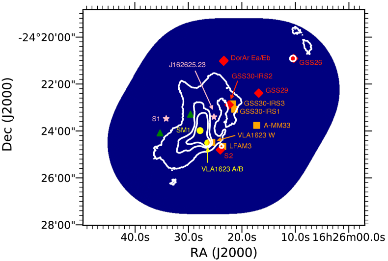
Figure 1: Field of view covered by the VLA X band observations in blue. The position of the detected Class 0, I, II and III sources are indicated with yellow circles, orange squares, red diamonds, and pink stars, respectively. Sources VLA1623 and DoAr 24E are binary systems. The extragalactic candidates are indicated with green triangles. White contours represent 850 $\mu$m continuum observations from the JCMT Gould Belt Survey taken by SCUBA-2 (Pattle et al., 2015; Kirk et al., 2018).

We calibrated the data manually using the CASA software package, following standard data calibration procedures. For maximizing our sensitivity, we combined the data from all five epochs of observation. We ensured that highly variable sources did not affect the image quality or the results by also imaging the individual epochs separately (see Sect. 3.2.2). The imaging was done with Briggs robust = 2.0 weighting, gridder = ‘mosaic’, specmode = ‘mfs’, and nterms = 1. This setting was used to maximize S/N ratios. Using ¿1 nterms is not suitable for this project given that the sources are relatively faint. At the average observing frequency, we obtained a synthesized beam of $\theta_{\mbox{\scriptsize{maj}}}$ $\times$ $\theta_{\mbox{\scriptsize{min}}}$ $\sim$ 0$\aas@@fstack{\prime\prime}$4 $\times$ 0$\aas@@fstack{\prime\prime}$2 and a maximum detectable angular scale of $\sim$5^′′ (or $\sim$700 au). After primary beam correction, we achieved a root-mean-square (RMS) noise level of $\sim$5 $\mu$Jy beam^-1 at the center of our mosaic field, which degrades to $\sim$28 $\mu$Jy beam^-1 toward the edges of the mosaic. The flux calibration uncertainty is expected to be about 5%.

Table 1: List of VLA observations

Epoch	Starting Time	Initial API rms	Projected baseline	$F^{\mbox{\scriptsize gain}}_{\mbox{\scriptsize 9.9 GHz}}$
	(UTC)	(∘)	(m)	(Jy)
1	2016-12-02 21:31	11	310-34300	1.4
2	2016-12-05 21:18	6.0	460-34300	1.3
3	2017-01-06 18:05	13	325-32800	1.4
4	2017-01-14 18:40	13	310-34300	1.3
5	2017-01-22 17:12	4.4	665-33100	1.3

Table 2: List of the mosaic pointings

Name	R.A.	Decl.
	(J2000)	(J2000)
X1	16${}^{\mbox{\tiny h}}$26${}^{\mbox{\tiny m}}$32${}^{\mbox{\tiny s}}$.00	-24∘24′30$\aas@@fstack{\prime\prime}$0
X2	16${}^{\mbox{\tiny h}}$26${}^{\mbox{\tiny m}}$20${}^{\mbox{\tiny s}}$.62	-24∘24′30$\aas@@fstack{\prime\prime}$0
X3	16${}^{\mbox{\tiny h}}$26${}^{\mbox{\tiny m}}$26${}^{\mbox{\tiny s}}$.31	-24∘22′15$\aas@@fstack{\prime\prime}$0
X4	16${}^{\mbox{\tiny h}}$26${}^{\mbox{\tiny m}}$14${}^{\mbox{\tiny s}}$.93	-24∘22′15$\aas@@fstack{\prime\prime}$0

3 Results

3.1 Source census and comparison with other surveys

In total, we detect 18 sources above 5$\sigma$ in our mosaic field of view. The fluxes of the detected sources were measured by performing two-dimensional Gaussian fits, using the imfit task of CASA. The derived fluxes and coordinates can be found in Table LABEL:table_catalog, where the names of the sources Jhhmmss.ss-ddmmss.s are based on the coordinates of peak intensity obtained with the fitting procedure. The position uncertainties are typically about a few tens of mas. Table LABEL:table_catalog also lists the more commonly used names of these sources. When the source structure was too complex to be fitted with this method or the results of the fit were too uncertain, we measured the flux by integrating over a circular area around the source with CASA. Table 6 summarizes the sizes measured with the Gaussian fit after deconvolution from the beam.

We compared our detections with the list of YSOs present in our field based on the photometric and spectroscopic surveys presented in Wilking et al. (2008), Jørgensen et al. (2008), Hsieh & Lai (2013), and Dzib et al. (2013). Previously Dzib et al. (2013) carried out large-scale observations of the Ophiuchus region with the VLA at 4.5 GHz and 7.5 GHz with a resolution of 1$\arcsec$. Wilking et al. (2008) used X-ray and infrared photometric surveys as well as spectroscopic surveys of the L1688 cloud to list all the association members present in the Two Micron All-Sky Survey (2MASS) catalog. They also classified the sources according to their respective spectral energy distributions (SEDs) built from the Spitzer Cores to Disks (c2d) survey. Hsieh & Lai (2013) compiled another list based on the c2d Legacy Project after developing a new method to identify fainter YSOs based on analyzing multi-dimensional magnitude space. Finally, Jørgensen et al. (2008) identified the more deeply embedded YSOs by jointly analyzing Spitzer and JCMT/SCUBA data. Our 18 detected sources have all been found in at least one earlier catalog or study. Specifically, 16 of our 18 radio detections are associated with YSOs, while the remaining two are probably extragalactic sources (Dzib et al., 2013). Individual images of our detected YSOs are provided in Figure 2. Sidelobes are visible for some of these sources (S1, SM1). In total, we detect 11 YSO candidates listed in the catalog of Wilking et al. (2008), while the remaining 19 YSOs in that catalog are undetected (see label ”b” in Table LABEL:table_catalog). Also, we detected nine of the sources listed by Hsieh & Lai (2013, see label ”c” in Table LABEL:table_catalog). Finally, we detected five of the young sources listed in Jørgensen et al. (2008), while two others (162614.63-242507.5 and 162625.49-242301.6) are undetected.

Compared to the previous VLA survey at 4.5 GHz and 7.5 GHz by Dzib et al. (2013, see Table LABEL:table_catalog), we detect seven additional radio sources, namely J162627.83-242359.4 (SM1, #3 in Table LABEL:table_catalog), J162617.23-242345.7 (A-MM33, #4), J162621.36-242304.7 (GSS30-IRS1, #5), J162623.36-242059.9 (DoAr 24Ea, #19), J162623.42-242102.0 (DoAr 24Eb, #20), J162624.04-242448.5 (S2, #21), and J162625.23-242324.3 (#30). All of these are young stellar objects. Three sources reported in Dzib et al. (2013) are undetected in our observations. These three sources are extragalactic (EG) candidates. A possible explanation for these non-detections is that they have a negative spectral index. Hence, the observations at 4.5 GHz and 7.5 GHz by Dzib et al. (2013) could be more sensitive to this type of targets because of their higher brightness at lower frequency. Another explanation would be that these sources are variable. We will now comment briefly on some of the individual young stellar objects.

J162627.83-242359.3 (also known as SM1, #3) was previously classified as a prestellar core (see Motte et al. 1998). It was, however, detected at 5 GHz with the VLA at an angular resolution of $\sim$10$\arcsec$ (measured peak fluxes of 130 – 200 $\mu$Jy beam^-1; Leous et al. 1991; Gagné et al. 2004), although, in the first study, the source appears slightly offset by 3$\arcsec$. More recent ALMA observations suggest that SM1 is actually protostellar and that it hosts a warm ($\sim$30–50 K) accretion disk or pseudo-disk (Friesen et al., 2014; Kirk et al., 2017; Friesen et al., 2018).

The source J162623.42-242101.9 (known as DoAr 24Eb, #20) is the companion of the protostar J162623.36-242059.9 (DoAr 24Ea, #19), also detected in our dataset (see Figure 2). These two sources are assumed to be at a similar evolutionary stage, although more data are needed to confirm this hypothesis (Kruger et al., 2012).

The source J162634.17-242328.7 (S1, #32) was suggested to be a binary separated by 20-30 mas (see discussion in Ortiz-León et al. 2017). Our VLA X band image does not spatially resolve the individual binary components. We note that the secondary component was not detected in the most recent epochs covered by Ortiz-León et al. (2017).

For the sources that we did not detect, we evaluated the 3$\sigma$ upper limits, which vary across the mosaic field due to primary beam attenuation (see Table LABEL:table_catalog). For 3 $\sigma$ RMS levels as low as $\sim$15 $\mu$Jy beam^-1, the detection statistics at 10 GHz in this region are 3/3 for Class 0 sources (100%), 5/8 for Class I YSOs (63%), 6/16 Class II sources (38%), and 2/5 Class III objects (40%).

Figure 3 shows the radio emission properties of the YSOs versus their Spitzer [3.6]-[4.5] colors (Evans et al., 2009). We see that the measured fluxes at 10 GHz of some sources are significantly brighter than the fluxes measured at 7.5 GHz by Dzib et al. (2013), while for other sources it is the opposite. The absence of systematic trend indicates that our data are probably not affected by flux calibration issues. We note that the classification of the continuous evolution of YSOs into Class 0/I, II, and III stages, taken from the literature, is to some extent artificial, and can be uncertain for YSOs that are transitioning from one stage to another. In addition, different catalogs or databases may report slightly different classifications, which are noted in Table LABEL:table_catalog.

3.2 Nature of the emission at 10 GHz

In this section, we evaluate how much of the flux measured towards the YSOs in our 10 GHz VLA observations is due to (i) thermal emission from dust, and (ii) other mechanisms such as free-free emission from ionized radio jets or photoevaporative winds, gyro-synchrotron emission from active magnetospheres, and synchrotron emission produced through the acceleration of cosmic-rays by jet or protostellar surface shocks (e.g., Macías et al. 2016; Gibb 1999; Forbrich et al. 2007; Padovani et al. 2016; Padovani & Galli 2018).

Table 3: Catalog of sources observed in the field of view of our observations grouped in categories.

#	Source0	Flux (mJy)1	Flux (mJy)1	Flux (mJy)1	Flux (mJy)1	Source	Ref.3	Variable4	$L_{X}$5	Other names
	(J2000 coordinates)	10.0 GHz	7.5 GHz	4.5 GHz	107 GHz	type2			(1029 erg s-1)
1	J162626.31-242430.7	0.485 $\pm$ 0.033	0.189 $\pm$ 0.034	0.189 $\pm$ 0.034	59.82 $\pm$ 0.471	YSO 0?8	a	Y		VLA1623 B
2	J162626.39-242430.8	0.289 $\pm$ 0.030	0.125 $\pm$ 0.025	0.087 $\pm$ 0.030	59.82 $\pm$ 0.471	YSO 0	a	U		VLA1623 A
3	J162627.83-242359.4	0.2307	$\lesssim$0.051	$\lesssim$0.051	23.13 $\pm$ 0.46	YSO/PC9	b			SM1
4	J162617.23-242345.7	0.1407	$\lesssim$0.051	$\lesssim$0.051	14.46 $\pm$ 0.29	YSO I	c,d			A-MM33, CRBR12,
										ISO-Oph 21
5	J162621.36-242304.7	0.1207	$\lesssim$0.051	$\lesssim$0.051	3.48 $\pm$ 0.67	YSO I/0-I	c/d			GSS 30-IRS1, Elias 21
6	J162621.72-242250.9	0.364 $\pm$ 0.030	0.304 $\pm$ 0.029	0.238 $\pm$ 0.017	30.71 $\pm$ 0.63	YSO I/FS	a/c	Y4.5GHz10		GSS 30-IRS3, LFAM1
7	162622.27-242407.1	$\lesssim$ 0.015	$\lesssim$0.051	$\lesssim$0.051	$\lesssim$0.16	YSO I-FS	c			CRBR25
8	J162623.58-242439.9	0.237 $\pm$ 0.035	$<$ 0.06	0.125 $\pm$ 0.015	$\lesssim$0.16	YSO 0-I/FS	d/a,c	Y	10.8	LFAM 3
9	162625.49-242301.6	$\lesssim$ 0.015	$\lesssim$0.051	$\lesssim$0.051	9.17 $\pm$ 0.44	YSO I	c			CRBR36
10	J162625.63-242429.4	0.277 $\pm$ 0.041	0.198 $\pm$ 0.023	0.218 $\pm$ 0.014	11.24 $\pm$ 0.44	YSO I	a,d	Y7.5GHz10		VLA1623 W, LFAM 4
11	162630.47-242257.1	$\lesssim$ 0.021	$\lesssim$0.051	$\lesssim$0.051	11.22 $\pm$ 0.44	YSO FS/0-I	c/d		4.8	$\ldots$
12	J162610.32-242054.9	0.3077	0.160 $\pm$ 0.022	0.100 $\pm$ 0.012	27.25 $\pm$ 0.35	YSO II	a,c,d	Y	9.5	GSS 26
13	J162616.85-242223.5	0.0707	0.360 $\pm$ 0.024	0.337 $\pm$ 0.017	$\lesssim$0.16	YSO II	a,c,d	Y	16.3	GSS 29, LFAM p1
14	162617.06-242021.6	$\lesssim$ 0.030	$\lesssim$0.051	$\lesssim$0.051	$\lesssim$0.16	YSO II	c		10.7	DoAr 24
15	162618.82-242610.5	$\lesssim$ 0.030	$\lesssim$0.051	$\lesssim$0.051	$\lesssim$0.16	YSO II	c			$\ldots$
16	162618.98-242414.3	$\lesssim$ 0.015	$\lesssim$0.051	$\lesssim$0.051	5.96 $\pm$ 0.98	YSO II-FS	c			CRBR15
17	162621.53-242601.0	$\lesssim$ 0.030	$\lesssim$0.051	$\lesssim$0.051	$\ldots$	YSO II	c		0.1–0.6	$\ldots$
18	J162622.39-242253.4	0.292 $\pm$ 0.027	1.42 $\pm$ 0.07	2.02 $\pm$ 0.10	$\lesssim$0.16	YSO II	a,c	Y	51.5	GSS 30-IRS2, VSSG12,
										ISO-Oph 34, LFAM 2
19	J162623.36-242059.96	0.1887	$\lesssim$0.051	$\lesssim$0.051	$\ldots$	YSO II	c,d		4.7	GSS 31a, DoAr 24Ea
20	J162623.42-242102.0	0.0857	$\lesssim$0.051	$\lesssim$0.051	$\ldots$	YSO II?	e			GSS 31b, DoAr 24Eb
21	J162624.04-242448.5	0.115 $\pm$ 0.027	$\lesssim$0.051	$\lesssim$0.051	$\lesssim$0.16	YSO II/FS	c/d		29.2	S2
22	J162625.28-242445.411	$\lesssim$ 0.024	$\lesssim$0.051	$\lesssim$0.051	$\lesssim$0.16	YSO II	c		0.5	$\ldots$
23	162627.81-242641.8	$\lesssim$ 0.036	$\lesssim$0.051	$\lesssim$0.051	$\ldots$	YSO II	c			$\ldots$
24	162637.79-242300.7	$\lesssim$ 0.042	$\lesssim$0.051	$\lesssim$0.051	$\lesssim$0.16	YSO II	c			LFAM p2
25	162642.74-242427.7	$\lesssim$ 0.060	$\lesssim$0.051	$\lesssim$0.051	$\lesssim$0.16	YSO II	c			$\ldots$
26	162642.89-242259.1	$\lesssim$ 0.069	$\lesssim$0.051	$\lesssim$0.051	$\lesssim$0.16	YSO II	c			$\ldots$
27	162643.86-242450.7	$\lesssim$ 0.084	$\lesssim$0.051	$\lesssim$0.051	$\lesssim$0.16	YSO II	c			$\ldots$
28	162615.81-241922.1	$\lesssim$ 0.063	$\lesssim$0.051	$\lesssim$0.051	$\lesssim$0.16	YSO III	c		3.1	$\ldots$
29	162622.19-242352.4	$\lesssim$ 0.015	$\lesssim$0.051	$\lesssim$0.051	$\lesssim$0.16	YSO III	c			$\ldots$
30	J162625.23-242324.3	0.0817	$\lesssim$0.051	$\lesssim$0.051	$\lesssim$0.16	YSO III/FS	c/d		6.0	$\ldots$
31	162631.36-242530.2	$\lesssim$ 0.024	$\lesssim$0.051	$\lesssim$0.051	$\lesssim$0.16	YSO III	c		0.2	$\ldots$
32	J162634.17-242328.7	7.75 $\pm$ 0.11	7.07 $\pm$ 0.35	7.98 $\pm$ 0.40	$\lesssim$0.16	YSO III	a,c	N	22.6	S1
33	162614.63-242507.5	$\lesssim$ 0.024	$\lesssim$0.051	$\lesssim$0.051	$\lesssim$0.16	YSO U	f			$\ldots$
34	162625.99-242340.5	$\lesssim$ 0.015	$\lesssim$0.051	$\lesssim$0.051	$\lesssim$0.16	YSO U	g			$\ldots$
35	162632.53-242635.4	$\lesssim$ 0.045	$\lesssim$0.051	$\lesssim$0.051	$\lesssim$0.16	YSO U	c			CRBR40
36	162638.80-242322.7	$\lesssim$ 0.045	$\lesssim$0.051	$\lesssim$0.051	$\ldots$	YSO U	c			$\ldots$
37	162639.92-242233.4	$\lesssim$ 0.078	$\lesssim$0.051	$\lesssim$0.051	$\ldots$	YSO U	c			$\ldots$
38	162608.04-242523.1	$\lesssim$ 0.051	$\leq$0.05	0.103 $\pm$ 0.014		EG?	a	Y
39	J162629.62-242317.3	0.0914	0.124 $\pm$ 0.018	0.228 $\pm$ 0.014		EG?	a	Y
40	J162630.59-242023.0	$\lesssim$ 0.045	0.064 $\pm$ 0.017	0.098 $\pm$ 0.013		EG?	a	Y
#	Source0	Flux (mJy)1	Flux (mJy)1	Flux (mJy)1	Flux (mJy)1	Source	Ref.3	Variable4	$L_{X}$5	Other names
	(J2000 coordinates)	10.0 GHz	7.5 GHz	4.5 GHz	107 GHz	type2			(1029 erg s-1)
41	J162634.95-242655.3	$\lesssim$ 0.069	0.100 $\pm$ 0.013	0.197 $\pm$ 0.019		EG?	a	Y
42	J162635.33-242405.3	0.377 $\pm$ 0.039	0.329 $\pm$ 0.033	0.650 $\pm$ 0.038		EG?	a	Y

Figure 2: Continuum observations of the detected young stellar objects with the VLA in band X. For all sources except S1, the contours start from 5$\sigma$ with a step of 5$\sigma$. For S1, the contours are 10$\sigma$, 20$\sigma$, 50$\sigma$, 100$\sigma$, and 200$\sigma$. The greyscale images start at 3$\sigma$. The red dot corresponds to the coordinates used to name the sources in Table LABEL:table_catalog. The last map (J162625.28-242445.4) is for epoch 3 only.

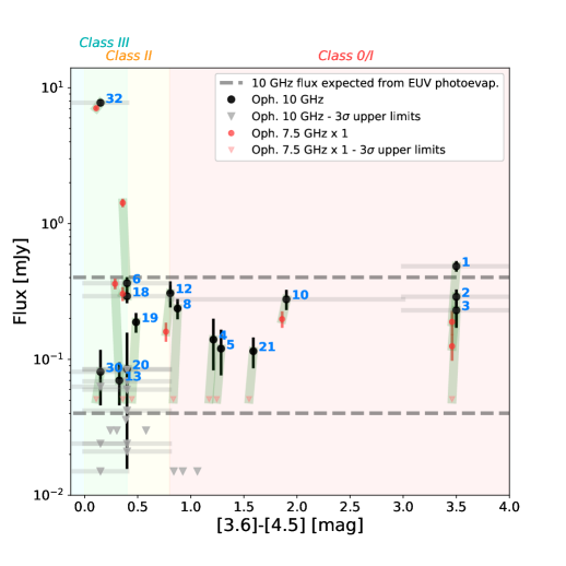
Figure 3: Summary of the observed 10 GHz radio fluxes. We show the characteristic [3.6]-[4.5] color ranges of the Class III, II, and 0/I YSOs as blue, yellow, and red filled regions which are bounded in the horizontal axis by [-0.4, 0.4], [0.0, 0.8], and [0.8, 4.0], respectively (the overlapped area for Class III and II objects appears in green; see Allen et al. 2004). Our 10 GHz detections are presented as black circles. For sources that we detected at 10 GHz, we also present the fluxes measured at 7.5 GHz (red symbols) by Dzib et al. (2013). For presentation purposes, we offset the [3.6]-[4.5] values of the red symbols by -0.04. The observations towards the same target sources are linked by green lines. Gray and red downward triangles are the 3$\sigma$ upper limits from these observations. Dashed lines show the expected radio fluxes from EUV photoevaporation winds from protoplanetary disks, assuming the EUV flux $\Phi_{\rm EUV}=$10⁴¹ (bottom) and 10⁴² photons s^-1 (top).

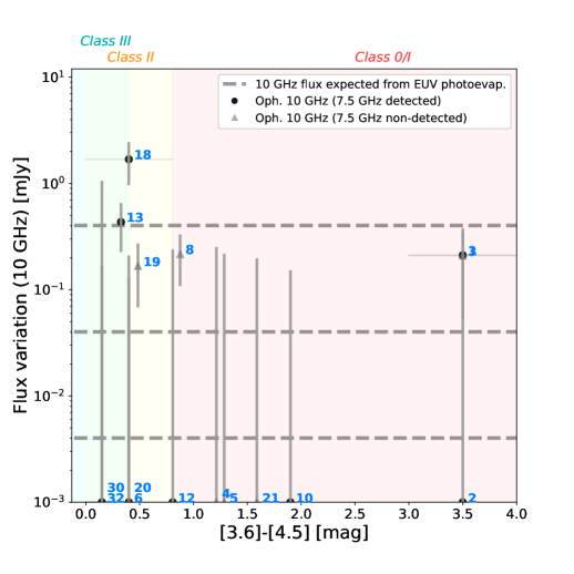
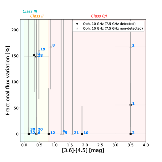
Figure 4: Summary of the observed radio flux variability (left panel) and fractional radio flux variability (right panel). We omit sources which were not detected in both our 10 GHz observations and the previous 7.5 GHz observations of Dzib et al. (2013), since there is essentially no constraint on their time variability. For sources which were detected from at least one of those observations, we present the flux variation by calculating the average of the differences between the measured 10 GHz flux in our VLA observations and the expected 10 GHz flux derived by re-scaling the 7.5 GHz flux from Dzib et al. (2013) to 10 GHz assuming $\alpha=$-0.1 and 2.0. Vertical error bars take the measurement errors and the spectral index range [-0.1, 2.0] into consideration. Dashed lines in the left panel show the expected radio fluxes from EUV photoevaporation winds from protoplanetary disks, assuming the EUV flux $\Phi_{\rm EUV}=$10⁴⁰ (bottom), 10⁴¹ (middle), and 10⁴² photons s^-1 (top).

The brightest source in our sample, J162634.17-242328.7 (S1, #32), has been already investigated in several studies and is known to be a completely non-thermal source. There is no evidence of a free-free component (e.g., André et al., 1988; Loinard et al., 2008; Ortiz-León et al., 2017). Indeed, the flux measured with the Very Long Baseline Array (VLBA) is systematically found to be equal to the VLA flux (Loinard et al., 2008; Ortiz-León et al., 2017). Since the VLBA is only sensitive to non-thermal emission whereas the VLA is in principle sensitive to both thermal and non-thermal emission (e.g., Ortiz-León et al., 2017), the emission of this source is confirmed here to be fully non-thermal. This source is, however, quite peculiar, since the non-thermal emission is not strongly variable, as confirmed with our observations (see Table LABEL:table_catalog). This result is somewhat of a mystery, and may be due to a magnetic field that, in this specific case, is fossil-based rather than dynamo driven (André et al., 1988). The former would explain S1’s lack of flaring activity that is otherwise typically seen in non-thermal sources. Given these extended studies focused on the S1 source, we do not discuss it further.

3.2.1 Contribution of the thermal emission from dust

To determine the thermal contribution from dust, we assume that the $\sim$107 GHz continuum fluxes reported by Kirk et al. (2017) are entirely due to dust thermal emission, and then extrapolate the contribution of dust emission at our observing frequency of 10 GHz by assuming a power-law with a spectral index $\alpha$ (see Table LABEL:table_catalog). We note that the angular resolution of the observations reported by Kirk et al. (2017) is approximately 10 times coarser than that of our VLA observations. Therefore, our estimates of 10 GHz dust emission should be regarded as upper limits.

In the millimeter bands (e.g., $\sim$90–350 GHz), the spectral indices of Class 0/I objects may be $\alpha$=2.5–3 (see Chiang et al. 2012; Tobin et al. 2013, 2015; Miotello et al. 2014), while those of Class II/III objects may become lower ($\alpha$=2–2.5; Ricci et al. 2010; Pérez et al. 2012; Tazzari et al. 2016) due to dust grain growth or high optical depths (see Li et al. 2017; Galván-Madrid et al. 2018). Taking this difference into account, we find that dust thermal emission could account for up to $\sim$30% of the observed 10 GHz flux toward the Class 0 YSOs and is almost negligible in the Class III objects of our sample. For the Class I/II YSOs, the situation is more complex. In general, the contribution of the dust emission is $\leq$30% and in some cases negligible. Exceptions, however, include the Class II sources J162610.32-242054.9 (also known as GSS26, #12), for which dust emission could account for $\sim$80% of the continuum flux at 10 GHz, and 162618.98-242414.3 (also called CRBR15, #16), for which the predicted dust emission is higher than the upper limit of 15 $\mu$Jy beam^-1, as well as two Class I sources (162625.49-242301.6, #9 and 162630.47-242257.1, #11), for which the predicted dust emission fluxes are comparable to the measured upper limits of 15 $\mu$Jy beam^-1 at 10 GHz. Therefore, except for a few Class I/II sources, the contribution from dust is in general $\leq$30% of the total emission. This behavior is consistent with even higher-angular resolution 870 $\mu$m ALMA observations toward the Class II sources J162623.36-242059.9 (#19) and J162623.42-242101.9 (#20, Cox et al., 2017), for which the dust contribution at 10 GHz is also estimated to be $\leq$30% assuming dust spectral indices $\alpha$=2–2.5.

3.2.2 Nature of the remaining radio emission

The remaining radio fluxes likely have contributions from (thermal) free-free emission from ionized radio jets, (thermal) free-free emission due to photoevaporative winds (e.g., Macías et al., 2016) or (non-thermal) gyro-synchrotron emission from stellar magnetospheres (e.g., Gibb, 1999; Forbrich et al., 2007). Jet or protostellar surface shocks can also produce (non-thermal) synchrotron emission at our observing frequency, for example through the acceleration of cosmic-rays (Carrasco-González et al., 2010; Padovani et al., 2016; Anglada et al., 2018). These radio emission mechanisms present specific characteristics, which we describe below.

Free-free emission from thermal jets and (gyro-)synchrotron emission are known to be time variable (Forbrich et al., 2007; Dzib et al., 2013), but they may have very different characteristic timescales (Liu et al., 2014). Free-free emission may vary on time-scales from a few weeks to a few months considering the ionized gas recombination timescales as well as the dynamical timescales of the inner $\sim$1 au disk. Gyro-synchrotron emission, however, is expected to vary on shorter timescales (minutes) due to flares on a stellar surface, and can vary up to the rotational periods of protostars. These periods can be as long as $\sim$10 days, due to large magnetic loops coupling protostars and their inner disks (Forbrich et al., 2007; Liu et al., 2014). Synchrotron emission is also expected to be variable, although the timescale is unclear (Padovani et al., 2016).

Observations also indicate that the fluxes of thermal (free-free) sources vary rarely more than 20–30%, while, in general, non-thermal sources show larger variability (Ortiz-León et al., 2017; Tychoniec et al., 2018). The spectral indices of each type of emission can also differ. Free-free emission is characterized by spectral indices in the range [-0.1, 2.0], while gyro-synchrotron emission can span a significantly larger range of -5 to +2.5. Spectral indices $<$ -0.4 have been observed in YSO jets and attributed to synchrotron emission (Anglada et al., 2018).

To probe the origins of the detected emission, we first checked if any of our sources were also detected with the VLBA. As explained at the beginning of Section 3.2, any detection with the VLBA is necessarily non-thermal. In addition to S1, three other sources present in our observations: J162616.85-242223.5 (GSS 29, #13), J162622.39-242253.4 (GSS 30-IRS2, #18), and J162625.63-242429.4 (VLA1623 W, #10) are detected at 5 GHz with the VLBA (Ortiz-León et al., 2017) but they are undetected at 8 GHz (see Table 4). By comparing the VLBA fluxes to the VLA fluxes measured by Dzib et al. (2013), we find that the emission of J162616.85-242223.5 (#13) could be fully non-thermal at 5 GHz. Unfortunately, no flux is available at 8 GHz for this source and we cannot rule out a fully non-thermal emission at 10 GHz. The emission of J162622.39-242253.4 (#18) could only be partially non-thermal, as the VLBA flux is lower than the VLA flux (19% at 5 GHz and $<$6% at 8 GHz). Nevertheless it has to be considered cautiously, since this source is possibly highly variable (Dzib et al., 2013) and the observations were not carried out at similar dates. The emission of J162625.63-242429.4 (#10) could be fully non-thermal, since at 5 GHz the VLBA emission is higher than the VLA flux and the VLBA upper limit at 8 GHz is not even a factor of 2 lower than the VLA measurement.

Table 4: Comparison of fluxes (mJy) measured towards 3 YSOs with the VLBA and the VLA.

#	Source	VLBAb	VLAc	VLBAb	VLAc
		5 GHz	5 GHz	8 GHz	8 GHz
10	J162625.63-242429.4	0.66	0.22	$<$0.12	0.20
13	J162616.85-242223.5	0.15–0.47a	0.34	$\ldots$	0.36
18	J162622.39-242253.4	0.30–0.38a	2.02	$<$0.09	1.42

Next, we determined the spectral indices of all sources between 10 GHz and 7.5 GHz and between 10 GHz and 4.5 GHz, taking into account both the fit uncertainty and the calibration uncertainty (see column 3 in Table 5). The only two sources with negative spectral indices (J162616.85-242223.5, #13 and J162622.39-242253.4, #18) are the ones detected with the VLBA, which confirms the non-thermal origin of these sources’ emission. Four sources, J162626.31-242430.7 (#1), J162627.83-242359.4 (#3), J162623.58-242439.9 (#8), and J162623.36-242059.9 (#19), show spectral indices higher than 2.5, which may indicate variability (see below).

Finally, we explored the long-term variability of the YSOs. Our observations were averaged over a couple of months and compared with those of Dzib et al. (2013) obtained in 2011. Dzib et al. (2013) reported that seven out of the 16 YSOs we detected are variable (see Table LABEL:table_catalog, column 9). We note that among these variable sources, two are those with spectral indices between 7.5 GHz and 10 GHz higher than 2.5. They also include the sources of non-thermal emission detected with the VLBA.

Any short-term variability will be explored in another paper by analyzing separately the 5 epochs as well as more recent observations at lower spatial resolution. Nevertheless, to ensure that our conclusions are not affected by significant variability, we separately checked the maps of the different epochs. As expected, the faintest sources are barely detected or not detected depending on the noise level of each epoch. Among the brightest sources, even if some variations are observed for some of them, the fluxes vary around the values measured in the map with the combined epochs. We did not see cases where the flux is significantly higher at one epoch. The only exception is found for the source J162625.8-242445.0 (#22) that is not detected in the map with the combined epochs, but clearly detected in epoch 3 with a flux of 0.4 mJy (see Figure 2), which is probably due to a non-thermal flare.

To explore possible radio flux variations since the observations of Dzib et al. (2013), we extrapolated their fluxes at 7.5 GHz to those at 10 GHz assuming that $\alpha$ is in the range of [-0.1, 2.0] (i.e., free-free emission from optically thin to optically thick limits) and compared the resulting values to our measured fluxes. For sources which were not detected at 7.5 GHz by Dzib et al. (2013), we evaluated the corresponding 3 $\sigma$ limits at 10 GHz assuming $\alpha$=2.0, and compared the resulting values with our measurements (see Figure 4). We found that there are three sources (J162626.31-242430.7/#1, J162616.85-242223.5/#13, and J162622.39-242253.4/#18) detected in both our 10 GHz observations and the previous 7.5 GHz observations, for which the flux differences are too large to be explained by constant free-free emission. The emission of J162616.85-242223.5 (#13), and J162622.39-242253.4 (#18) is certainly non-thermal, as explained before. The emission of J162626.31-242430.7 (#1) may be explained either by non-thermal radio emission or by thermal radio flux variability of more than a few tens of percent (see Figure 4). In addition, after considering the spectral index range [-0.1, 2.0], it appears that three of our new radio detections (J162627.83-242359.4/#3, J162623.58-242439.9/#8, and J162623.36-242059.9/#19) cannot be attributed to our improved sensitivity. The measured 10 GHz fluxes in the new VLA observations are significantly larger than 10 GHz fluxes scaled from the 7.5 GHz upper limit fluxes of Dzib et al. (2013, see Figure 4). Therefore, these detections are either due to variability or non-thermal, gyro-synchrotron spectral indices. The fractional radio flux variability of the sources can be seen in Figure 4. We find that six out of our detected sources in the [3.6]-[4.5] color range of [0, 2] (i.e., late Class 0/I to early Class III stages) show over 50% fractional radio flux variability. The absolute values of their flux variations appear comparable to the observed flux variations from five epochs of observations towards CrA on the same date (Liu et al., 2014). The radio emission of some of these six sources (including J162625.63-242429.4/#10, 162616.85-242223.5/#13, and J162622.39-242253.4/#18) may be largely contributed by gyro-synchrotron emission which can vary on short timescales.

Table 5 summarizes our conclusions regarding the radio emission of the Oph A YSOs.

Table 5: Summary of the emission of the YSOs.

#	Source	Spectral	Dust	Ionized emission			X-ray	$\phi$EUV6
		index		VLBA	Variability3	Fully or	detection5	(1040
		$\alpha$1		detection		partially		erg s-1)
				at 5 GHz2		non-thermal
						emission4
Class 0
1	J162626.31-242430.7	3.3$\pm$0.7 / 1.2$\pm$0.3	$\leq$ 21%	N	Y	Y
2	J162626.39-242430.8	2.9$\pm$0.8 / 1.5$\pm$0.5	$\leq$ 21%	N
3	J162627.83-242359.3	$\geq$4.8 / $\geq$1.7	$\leq$ 27%		Y	Y
Class I
4	J162617.24-242346.0	$\geq$2.9 / $\geq$1.7	$\leq$ 28%
5	J162621.36-242304.7	$\geq$2.3 / $\geq$1.0	$\leq$ 8%
6	J162621.72-242250.9	0.6$\pm$0.5 / 0.5$\pm$0.2	$\leq$ 23%	N	Y4.5GHz†	Y
7	162622.27-242407.1	$\ldots$	$\ldots$
8	J162623.58-242439.9	$>$4.2 / 0.8$\pm$0.3	$\leq$ 0.2%	N	Y	Y	Y
9	162625.49-242301.6	$\ldots$	$\leq$ 100%
10	J162625.63-242429.4	1.2$\pm$0.7 / 0.3$\pm$0.2	$\leq$ 10%	Y	Y7.5GHz†	Y
11	162630.47-242257.1	$\ldots$	$\leq$ 100%				Y
Class II
12	J162610.32-242054.9	2.3$\pm$0.6 / 1.4$\pm$0.2	$\leq$ 77%	N	Y†	Y	Y	$<$74
13	J162616.85-242223.5	-5.7$\pm$1.0 / -1.9$\pm$0.4	$\leq$ 2%	Y	Y	Y	Y
14	162617.06-242021.6	$\ldots$	$\ldots$				Y	$\lesssim$7
15	162618.82-242610.5	$\ldots$	$\ldots$					$\lesssim$7
16	162618.98-242414.3	$\ldots$	$\leq$ 100%					$\lesssim$4
17	162621.53-242601.0	$\ldots$	$\ldots$				Y	$\lesssim$7
18	J162622.39-242253.4	-5.5$\pm$0.4 / -2.4$\pm$0.2	$\leq$ 0.5%	Y	Y	Y	Y	$<$71
19	J162623.36-242059.9	$\geq$4.0 / $\geq$1.4	$\leq$ 18%		Y	Y	Y	$<$45
20	J162623.42-242101.9	$\geq$0.8 / $\geq$0.3	$\leq$ 34%					$\lesssim$21
21	J162624.04-242448.5	$\geq$1.9 / $\geq$0.7	$\leq$ 1%				Y	$\lesssim$28
22	J162625.28-242445.4	$\ldots$	$\ldots$				Y	$\lesssim$6
23	162627.81-242641.8	$\ldots$	$\ldots$					$\lesssim$9
24	162637.79-242300.7	$\ldots$	$\ldots$					$\lesssim$10
25	162642.74-242427.7	$\ldots$	$\ldots$					$\lesssim$14
26	162642.89-242259.1	$\ldots$	$\ldots$					$\lesssim$17
27	162643.86-242450.7	$\ldots$	$\ldots$					$\lesssim$21
Class III
28	162615.81-241922.1	$\ldots$	$\ldots$				Y	$\lesssim$15
29	162622.19-242352.4	$\ldots$	$\ldots$					$\lesssim$4
30	J162625.23-242324.3	$\geq$0.3 / $\geq$0.1	$\leq$ 2%				Y	$\lesssim$20
31	162631.36-242530.2	$\ldots$	$\ldots$				Y	$\lesssim$6
32	J162634.17-242328.7	0.3$\pm$0.3 / 0.0$\pm$0.1	$\leq$ 0.02%	Y	N	Y	Y

3.2.3 Association with X-ray emission

We checked the sources associated with X-ray emission (Imanishi et al., 2003, see column 10 in Table LABEL:table_catalog). For Class III sources, X-ray emission mainly arises from magnetized stellar coronae, while in younger (Class I/II) sources, additional mechanisms can produce X-ray emission (e.g., shocks due to the material infalling from the disk to the stellar surface or due to the interaction of outflows with circumstellar material). All the Class II and III sources detected in our data are associated with X-ray emission, apart from J162623.42-242102.0 (DoAr 24Eb, #20). The spatial resolution of Chandra telescope might not be sufficient to separate its emission from J162623.36-242059.9 (DoAr 24Ea). Among the younger sources we detected, only the Class I object J162623.58-242439.9 (#8) is detected in X-ray.

4 Discussion: Revisiting photoevaporation in Class II/III proto-planetary disks

High energy stellar photons (UV or X-rays) may contribute to the dispersal of protoplanetary disks through photoevaporation (Hollenbach et al., 1994; Alexander et al., 2014). The exact contribution of this mechanism to disk dispersal and the way it impacts planet formation, however, need to be further investigated. Observations at radio wavelengths can probe the free-free emission from a disk surface that is partially or totally ionized by EUV photons or X-ray photons. Therefore, radio wavelength observations can be a powerful diagnostic of the contributions of these two types of photons in the protoplanetary disk evolution. For example, Pascucci et al. (2012) predict the level of radio emission expected from photoevaporation driven by EUV photons or X-ray photons. Based on an analysis of 14 circumstellar disks, Pascucci et al. (2014) then determined that the EUV photoevaporation mechanism may not play a significant role in disk mass dispersal, when EUV photon luminosities ($\Phi$ _EUV) are lower than 10⁴² photons s^-1. Similar conclusions were obtained by Galván-Madrid et al. (2014) for ten disks toward the Corona Australis (CrA) star-forming region, inferring $\Phi_{\rm EUV}$ ¡ (1–4) $\times$ 10⁴¹ photons s^-1, and by Macías et al. (2016) for the transitional disk of GM Aur ($\Phi_{\rm EUV}$ $\sim$ 6 $\times$ 10⁴⁰ photons s^-1).

4.1 Constraints on EUV disk photoevaporation

The high sensitivity of our observations (5 $\mu$Jy beam^-1 at the center of the field of view) and the proximity of this cloud (137 pc) allow us to derive stringent constraints on the contribution of EUV photons on disk photoevaporation in the Oph A star-forming region. As explained before, the radio emission of five of our detected Class II/III sources (J162610.32-242054.9/#12, J162616.85-242223.5/#13, J162622.39-242253.4/#18, J162623.36-242059.9/#19, and J162634.17-242328.7/#32) is probably fully or partially non-thermal and we cannot exclude it for the three other detected sources. As such, the best constraints come from the Class II/III objects we did not detect.

Following the approach of Pascucci et al. (2014) and Galván-Madrid et al. (2014), we estimate the expected radio continuum fluxes $F_{\mbox{\tiny 10 GHz}}$ for a particular EUV luminosity $\Phi_{\mbox{\tiny EUV}}$ based on the following formulation :

$$F_{\mbox{\tiny 10 GHz}}\mbox{ [$\mu$Jy]}\sim 4.0\times 10^{-40}\left(\frac{137}{d\mbox{ [pc]}}\right)^{2}\left(\Phi_{\mbox{\tiny EUV}}\mbox{ [s${}^{-1}$]}\right)\left(\frac{10.0}{8.5}\right)^{\alpha},$$ (1)

where $d$ is the distance of the target source, and $\alpha$ is the spectral index of the free-free emission produced by the EUV photoevaporation. As an approximation, we tentatively consider $\alpha$=0, and note that our estimate of $F_{\mbox{\tiny 10 GHz}}$ is not especially sensitive to the exact value of $\alpha$ as long as $\alpha$ is in the range of [-0.1, 2.0]. We provide the estimates of $F_{\mbox{\tiny 10 GHz}}$ at $\Phi_{\rm EUV}=$10⁴⁰, 10⁴¹, and 10⁴² photons s^-1 for Figures 3 and 4. For Class II and III sources which were not detected in our observations, the respective 3 $\sigma$ upper limits of $F_{\mbox{\tiny 10 GHz}}$ constrain their $\Phi_{\rm EUV}$ to be $\lesssim$ 4–21 $\times$ 10⁴⁰ photons s^-1 (Figure 3 and Table LABEL:table_catalog). These upper limits are lower than those derived from previous observations towards CrA (¡1–4 $\times$ 10⁴¹ photons s^-1, Galván-Madrid et al., 2014). We note that typical EUV photoevaporation models require $\Phi_{\rm EUV}$ to be in the range of 10⁴¹–10⁴² s^-1 to disperse protoplanetary disks within a few Myrs (Font et al., 2004; Alexander et al., 2006; Alexander & Armitage, 2009). EUV-driven photoevaporation is consequently very unlikely to play a major role in the dispersal of these disks.

For the Class II and III sources that are detected in our 10 GHz observations and do not necessarily exhibit non-thermal emission (J162623.42-242102.0/#20, J162624.04-242448.5/#21, and J162625.23-242324.3/#30), if we assume that their 10 GHz fluxes are dominated by photoevaporation winds, the corresponding $\Phi_{\rm EUV}$ values are well in the range required by the aforementioned models (Figure 3). Hence, photoevaporation driven by EUV photons could be sufficiently efficient to disperse these disks. Presently, however, we do not have good enough constraints about the spectral indices of these detected sources to tell what fractions of their radio fluxes come from constant EUV photoevaporation winds. Observationally, we also do not know yet whether the radio emission associated with EUV photo-evaporating disks evolves with time.

4.2 Constraints on X-ray disk photo-evaporation

Photoevaporation by X-ray photons is another process that may lead to the dispersal of protoplanetary disks. We listed in Table LABEL:table_catalog the observed X-ray luminosities found in the literature for the YSOs of Oph A (Imanishi et al., 2003). They range over 0.01–3 $\times$ 10³⁰ erg s^-1. Pascucci et al. (2012) determined the relation between the incident X-ray photon luminosity $L_{\mbox{\tiny X}}$ and the resulting free-free emission that a disk would emit:

$$F_{\mbox{\tiny 10 GHz}}\mbox{ [$\mu$Jy]}\sim 3.3\times 10^{-30}\left(\frac{137}{d\mbox{ [pc]}}\right)^{2}\left(L_{\mbox{\tiny X}}\mbox{ [erg s${}^{-1}$]}\right)\left(\frac{10.0}{8.5}\right)^{\alpha}.$$ (2)

Based on this equation and the level of non-detections in our Class II objects, the upper limits derived for the incident X-ray photon luminosity are $\lesssim$ (7–25) $\times$ 10³⁰ erg s^-1, i.e. about 1–2 orders of magnitude higher than the observed values on average. Thus, we cannot exclude, with the present data, X-ray photoevaporation as a major mechanism in the dispersal of the disks. More sensitive observations are needed to determine its efficiency.

4.3 Studying the photoevaporation of protoplanetary disks with the Square Kilometre Array

In the future, SKA will certainly revolutionize our understanding of the star and planet formation process through radio emission studies. We discuss here the potential of SKA to investigate the photoevaporation of disks.

The free-free emission produced by a disk (at the distance of Oph A) with an X ray luminosity of more than 10²⁹ erg s^-1 could be detected for example with an rms of 0.1 $\mu$Jy. Such a high sensitivity should be reached in the future with the SKA. In particular, Hoare et al. (2015) estimated that a 1000 hour deep field integration at the full resolution of SKA1-Mid ($\sim$40 mas, i.e. $\sim$5 AU for the disks of Oph A) over a 2 $\times$ 2.5 GHz bandwidth from 8.8 GHz to 13.8 GHz will yield a noise level of 0.07 $\mu$Jy beam^-1. Although the required amount of time appears significantly higher than the time dedicated to current radio projects, it should be noted that multiple projects will be carried out simultaneously with the SKA and that a large number of sources will be covered in the same field with a single pointing. For example, the investigation of the photoevaporation in disk dispersal can be carried out simultaneously with the high priority studies of grain growth and the search for prebiotic molecules (Hoare et al., 2015).

With a single pointing, the SKA will cover a field of view of about 6 arcminutes (comparable to our 4 pointing VLA mosaic). By targeting a rich region such as the Oph A cluster, a large number of disks (all the disks listed in this paper) can be observed simultaneously.

For bright radio emission sources, SKA will further provide good constraints on the instantaneous spectral indices over a wide range of frequency, useful data for gauging the fractional contributions of thermal and non-thermal emission mechanisms. An expansion of SKA1-Mid to $\sim$25 GHz would provide even stronger constraints on the spectral indices resolved across the young stars, spatially separating the different components. Complementary observations will also be possible with the next generation VLA (ng-VLA, Murphy et al. 2018; Selina et al. 2018) above the highest SKA1-Mid band.

In addition, shallow (e.g., RMS $\sim$ few $\mu$Jy) but regularly scheduled SKA monitoring surveys will provide for the first time the statistics of how much time Class 0-III YSOs are in the radio active or inactive states, and what the dominant radio emission mechanisms and radio flux variability levels are during these states.

Finally, the SKA1-Mid resolution will be around 40 mas and hence it will be possible to separate spatially the different contributions from flares, jet, wind and disk to some degree. Simultaneous observations of hydrogen radio recombination lines at the high-angular resolution of the SKA will also enable the separation of ionized gas emission from dust emission in disks, which will be key for these kinds of studies.

Getting photoevaporation rates should consequently be achievable with the power of SKA, however separating out the role of each type (EUV/X-ray) may be more complicated. According to Pascucci et al. (2012), the EUV contribution should be a factor 10 higher than the X-ray contribution. Photoevaporation models predict different mass-loss profiles, but the subtraction of the EUV contribution to the free-free emission (necessary to investigate the X-ray driven photoevaporation of disks) could turn out to be highly uncertain, since the EUV luminosity is unknown.

5 Conclusions

We carried out very sensitive continuum observations of the Oph A star-forming region at 10 GHz with the VLA (1 $\sigma$ = 5 $\mu$Jy beam^-1 at the center of the field of view). We detected sixteen YSOs and two extragalactic candidate sources. Seven of the detected YSOs were not detected in a previous VLA survey of this region at 4.5 GHz and 7.5 GHz by Dzib et al. (2013).

Using typical spectral indices for the possible components of radio emission, we constrained the origin of the emission detected at 10 GHz towards the YSOs. In general, dust emission contributes less than 30% of the total emission. The 10 GHz emission appears to be mainly due to gyro-synchrotron emission from active magnetospheres, free-free emission from thermal jets or photoevaporative winds, or synchrotron emission due to accelerated cosmic-rays. Three of the YSOs show evidence of non-thermal emission. A comparison with the survey by Dzib et al. (2013) shows that six of the sources show over 50% fractional radio flux variability, which is probably due to non-thermal emission.

Constraints on the EUV and X-ray photoevaporation mechanisms were discussed. For the Class II/III disks for which we detect no emission, the corresponding EUV luminosities are not sufficient to explain disk dispersal within a few Myrs through theoretical photoevaporation models. For the sources detected at 10 GHz (with a possibly significant contribution of ionized thermal emission), the corresponding maximum $\Phi_{\rm EUV}$ values are within the range predicted by models. It is, however, currently unclear if EUV photoevaporating winds and their contributions to radio fluxes are constant in time. Even with the very high sensitivity of our observations, we are unable to provide strong constraints on the efficiency of X-ray for disk dispersal. Significantly more sensitive observations that also resolve the sources are necessary to locate the different emission origins and constrain the efficiency of the photoevaporation mechanisms. With higher sensitivity and higher angular resolution, future facilities such as the Square Kilometre Array will make this possible.

Appendix A Image component sizes obtained with imfit.

Table 6: Image component sizes (deconvolved from beam) obtained with imfit.

#	Source	Major axis	Minor axis	Position
		FWHM ($\arcsec$)	FWHM ($\arcsec$)	angle ($\degree$)
1	J162626.31-242430.7	0.78$\pm$0.09	0.52$\pm$0.09	76$\pm$15
2	J162626.39-242430.8	0.83$\pm$0.14	0.45$\pm$0.11	67$\pm$16
6	J162621.72-242250.9	0.97$\pm$0.11	0.57$\pm$0.05	37$\pm$8
8	J162623.58-242439.9	0.94$\pm$0.20	0.75$\pm$0.14	36$\pm$77
10	J162625.63-242429.4	1.06$\pm$0.22	0.69$\pm$0.23	85$\pm$28
18	J162622.39-242253.4	1.08$\pm$0.14	0.52$\pm$0.05	26$\pm$6
21	J162624.04-242448.5	1.37$\pm$0.40	0.47$\pm$0.15	52$\pm$12
32	J162634.17-242328.7	0.65$\pm$0.02	0.09$\pm$0.01	25.6$\pm$0.5
42	J162635.33-242405.3	0.55$\pm$0.14	0.25$\pm$0.07	50 $\pm$16