A Generalized Configuration Model with Degree Correlations and Its Percolation Analysis

Abstract In this paper we present a generalization of the classical configuration model. Like the classical configuration model, the generalized configuration model allows users to specify an arbitrary degree distribution. In our generalized configuration model, we partition the stubs in the configuration model into $b$ blocks of equal sizes and choose a permutation function $h$ for these blocks. In each block, we randomly designate a number proportional to $q$ of stubs as type 1 stubs, where $q$ is a parameter in the range $[0,1]$. Other stubs are designated as type 2 stubs. To construct a network, randomly select an unconnected stub. Suppose that this stub is in block $i$. If it is a type 1 stub, connect this stub to a randomly selected unconnected type 1 stub in block $h(i)$. If it is a type 2 stub, connect it to a randomly selected unconnected type 2 stub. We repeat this process until all stubs are connected. Under an assumption, we derive a closed form for the joint degree distribution of two random neighboring vertices in the constructed graph. Based on this joint degree distribution, we show that the Pearson degree correlation function is linear in $q$ for any fixed $b$. By properly choosing $h$, we show that our construction algorithm can create assortative networks as well as disassortative networks. We present a percolation analysis of this model. We verify our results by extensive computer simulations.

keywords: configuration model, assortative mixing, degree correlation

1 Introduction

Recent advances in the study of networks that arise in field of computer communications, social interactions, biology, economics, information systems, etc., indicate that these seemingly widely different networks possess a few common properties. Perhaps the most extensively studied properties are power-law degree distributions [1], the small-world property [29], network transitivity or ”clustering” [29]. Other important research subjects on networks include network resilience, existence of community structures, synchronization, spreading of information or epidemics. A fundamental issue relevant to all the above research issues is the correlation between properties of neighboring vertices. In the ecology and epidemiology literature, this correlation between neighboring vertices is called assortative mixing.

In general, assortative mixing is a concept that attempts to describe the correlation between properties of two connected vertices. Take social networks for example. vertices may have ages, weight, or wealthiness as their properties. It is found that friendship between individuals are strongly affected by age, race, income, or languages spoken by the individuals. If vertices with similar properties are more likely to be connected together, we say that the network shows assortative mixing. On the other hand, if vertices with different properties are likely to be connected together, we say that the network shows disassortative mixing. It is found that social networks tend to show assortative mixing, while technology networks, information networks and biological networks tend to show disassortative mixing [21]. The assortativity level of a network is commonly measured by a quantity proposed by Newman [20] called assortativity coefficient. If the assortativity level to be measured is degree, assortativity coefficient reduces to the standard Pearson correlation coefficient [20]. Specifically, let $X$ and $Y$ be the degrees of a pair of randomly selected neighboring vertices, the Pearson degree correlation function is the correlation coefficient of $X$ and $Y$, i.e.

$$\rho(X,Y)\stackrel{{\scriptstyle\scriptstyle\rm def}}{{=}}\frac{{\bf\sf E}(XY)-{\bf\sf E}(X){\bf\sf E}(Y)}{\sigma_{X}\sigma_{Y}},$$ (1)

where $\sigma_{X}$ and $\sigma_{Y}$ denote the standard deviation of $X$ and $Y$ respectively. We refer the reader to [20,21,12,30,22,3,17] for more information on assortativity coefficient and other related measures. In this paper we shall focus on degree as the vertex property.

Researchers have found that assortative mixing plays a crucial role in the dynamic processes, such as information or disease spreading, taking place on the topology defined by the network [18,3,7,17,26]. Assortativity also has a fundamental impact to the network resilience as the network loses vertices or edges [28]. In order to study information propagation or network resilience, researchers may need to build models with assortative mixing or disassortative mixing. Newman [20] and Xulvi-Brunet et al. [30] proposed algorithms to generate networks with assortative mixing or disassortative mixing based on an idea of rewiring edges. Boguñá et al. [3] proposed a class of random networks in which hidden variables are associated with the vertices of the networks. Establishment of edges are controlled by the hidden variables. Ramezanpour et al. [23] proposed a graph transformation method to convert a configuration model into a graph with degree correlations and non-vanishing clustering coefficients as the network grows in size. However, the degree distribution no longer remains the same as the network is transformed. Zhou [31] also proposed a method to generate networks with assortative mixing or disassortative mixing using a Monte Carlo sampling method. Comparing with these methods, our method has an advantage that specified degree distributions are preserved in the constructed networks. In addition, our method allows us to derive a closed form for the Pearson degree correlation function for two random neighboring vertices.

In this paper we propose a method to generate random networks that possess either assortative mixing property or disassortative mixing property. Our method is based on a modified construction method of the configuration model proposed by Bender et al. [2] and Molloy et al. [15]. The modified construction method is as follows. Given a degree distribution, generate a sequence of degrees. Each vertex is associated with a set of “stubs” where the number of stubs is equal to the degree of the vertex. We sort and arrange the stubs of all vertices in ascending order (descending order would be fine as well). Sort and divide the stubs into $b$ blocks. We associate each block with another block. This association forms a permutation, i.e. no two distinct blocks are associated with a common block. We randomly designate a fixed number of stubs in each block as type-1 stubs. The rest stubs are all designated as type-2 stubs. To connect stubs, we randomly select a stub. If it is a type-1 stub, we connect it to a randomly selected type-1 stub in the associated block. If it is a type-2 block, we connect it to a randomly selected type-2 stub out of all type-2 stubs. We repeat this process until all stubs are connected. To generate a generalized configuration model with assortative mixing property, we select permutation of blocks such that a block of stubs with large degrees is associated with another block of large degrees. To generate a network with disassortative mixing, we select permutation such that a block of large degrees is assciated with a block of small degrees. We present the detail of the construction algorithm in Section 2. For this model, we derive a closed form for the Pearson correlation coefficient of the degrees of two neighboring vertices. From the Pearson correlation coefficient of degrees we show that our constructed network can be assortative or disassortative as desired.

In this paper we present an application of the proposed random graph model. We consider a percolation analysis of the generalized configuration model. Percolation has been a powerful tool to study network resilience under breakdowns or attacks. Cohen et. al [6] studied the resilience of networks with scale-free degree distributions. Particularly, Cohen et. al studied the stability of such networks, including the Internet, subject to random crashes. Percolation has also been used to study disease spreading in epidemic networks [5,16,25]. Percolation has been used to study the effectiveness of immunization or quarantine to confine a disease. Schwartz et al. [27] studied percolation in a directed scale-free network. Newman [19] and Vázquez et al. [28] studied percolation in networks with degree correlation. Vázquez et al. assumed general random networks, their solution involves with the eigenvalues of a $D\times D$ matrix, where $D$ is the total number of degrees in the network. The percolation analysis of our model involves with solving roots of a simultaneous system of $b$ nonlinear equations, where $b$ is the number of blocks in the generalized configuration model. Since $b$ is typically a small integer, we have significantly reduced the complexity.

The rest of this paper is organized as follows. In Section 2 we present our construction method of a random network. In Section 3 we derive a closed form for the joint degree distribution of two randomly selected neighboring vertices from a network constructed by the algorithm in Section 2. In Section 4, we show that the Pearson degree correlation function of two neighboring vertices is linear. We then show how permutation function $h$ should be selected such that a constructed random graph is associatively or disassortatively mixed. In Section 5 we present a percolation analysis of this model. Numerical examples and simulation results are presented in Section 6. Finally, we give conclusions in Section 7.

2 Construction of a Random Network

Research on random networks was pioneered by Erdős and Rényi [8]. Although Erdős-Rényi’s model allows researchers to study many network problems, it is limited in that the vertex degree has a Poisson distribution asymptotically as the network grows in size. The configuration model [2,15] can be considered as an extension of the Erdős and Rényi model that allows general degree distributions. Configuration models have been used successfully to study the size of giant components. It has been used to study network resilience when vertices or edges are removed. It has also been used to study the epidemic spreading on networks. We refer the readers to [21] for more details. In this paper we propose an extension of the classical configuration model. This model generates networks with specified degree sequences. In addition, one can specify a positive or a negative degree correlation for the model. Let there be $n$ vertices and let $p_{k}$ be the probability that a randomly selected vertex has degree $k$. We sample the degree distribution $\{p_{k}\}$ $n$ times to obtain a degree sequence $k_{1},k_{2},\ldots,k_{n}$ for the $n$ vertices. We give each vertex $i$ a total of $k_{i}$ stubs. There are $2m=\sum_{i=1}^{n}k_{i}$ stubs totally, where $m$ is the number of edges of the network. In a classical configuration model, we randomly select an unconnected stub, say $s$, and connect it to another randomly selected unconnected stub in $[1,2m]-\{s\}$. We repeat this process until all stubs are connected. The resulting network can be viewed as a matching of the $2m$ stubs. Each possible matching occurs with equal probability. The consequence of this construction is that the degree correlation of a randomly selected pair of neighboring vertices is zero. To achieve nonzero degree correlation, we arrange the $2m$ stubs in ascending order (descending order will also work) according to the degree of the vertices, to which the stubs belong. We label the stubs accordingly. We partition the $2m$ stubs into $b$ blocks evenly. We select integer $b$ such that $2m$ is divisible by $b$. Each block has $2m/b$ stubs. Block $i$, where $i=1,2,\ldots,b$, contains stubs $(i-1)(2m/b)+j$ for $j=1,2,\ldots,2m/b$. Next, we choose a permutation function $h$ of $\{1,2,\ldots,b\}$. If $h(i)=j$, we say that block $j$ is associated with block $i$. In this paper we select $h$ such that

$$h(h(i))=i,$$

i.e., if blocks $i$ and $h(i)$ are mutually associated with each other. In each block, we randomly designate $\lceil 2mq/b\rceil$ stubs as type 1 stubs, where $q$ is a parameter in the range $[0,1)$. Other stubs are designated as type 2 stubs. Randomly select an unconnected stub. Suppose that this stub is in block $i$. If it is a type 1 stub, connect this stub to a randomly selected unconnected type 1 stub in block $h(i)$. If it is a type 2 stub, connect it to a randomly selected unconnected type 2 stub in $[1,2m]$. We repeat this process until all stubs are connected. The construction algorithm is shown in Algorithm 1.

Inputs: degree sequence $\{k_{i}:i=1,2,\ldots,n\}$;

Outputs: graph $(G,V,E)$;

Create $2m$ stubs arranged in descending order;

Divide $2m$ stubs into $b$ blocks evenly. Initially, all stubs are unconnected. For each block, randomly designate $\lceil 2mq/b\rceil$ stubs as type 1 stubs. All other stubs are designated as type 2 stubs;

while there are unconnected stubs do

       Randomly select a stub. Assume that the stub is in block $i$;

       if type 1 stub then

             connect this stub with a randomly selected unconnected type 1 stub in block $h(i)$;

            

      else

             connect this stub with a randomly selected unconnected type 2 stub in $[1,2m]$;

            

       end if

      

end while

Algorithm 1 Construction Algorithm

We make a few remarks. First, note that in networks constructed by this algorithm, there are $mq$ edges that have two type-1 stubs on their two sides. These edges create degree correlation in the network. On the other hand, there are $m(1-q)$ edges in the network that have two type-2 stubs on their two sides. These edges do not contribute towards degree correlation in the network. Second, random networks constructed by this algorithm possess the following property. A randomly selected stub connects to another randomly selected in the associated block with probability $q$. With probability $1-q$, this stub connects to a randomly selected stub in $[1,2m]$. Finally, note that standard configuration models can have multiple edges connecting two particular vertices. There can also be edges connecting a vertex to itself. These are called multiedges and self edges. In our constructed networks, multiedges and self edges can also exist. However, it is not difficult to show that the expected density of multiedges and self edges approaches to zero as $n$ becomes large. Due to space limit, we shall not address this issue in this paper.

3 Joint Distribution of Degrees

Consider a randomly selected edge in a random network constructed by the algorithm described in Section 2. In this section we analyze the joint degree distribution of the two vertices at the two ends of the edge.

We randomly select a vertex and let $Z$ be the degree of this vertex. Since the selection of vertices is random,

$$\Pr(Z=k_{i})=\frac{1}{n}$$

for $i=1,2,\ldots,n$. Thus, the expectation of $Z$ is

$${\bf\sf E}(Z)=\frac{\sum_{i=1}^{n}k_{i}}{n}=\frac{2m}{n}.$$

The expectation of $Z$ can also be expressed as

$${\bf\sf E}(Z)=\sum_{k=0}^{\infty}kp_{k}.$$ (2)

The expected number of stubs of the network is ${\bf\sf E}(Z)\cdot n$. We would like to evenly allocate these stubs into $b$ blocks such that each block has $n{\bf\sf E}(Z)/b$ stubs on average. We make the following assumption.

Assumption 1

The degree distribution $\{p_{k}\}$ is said to satisfy this assumption if one can find mutually disjoint sets $H_{1},H_{2},\ldots,H_{b}$, such that

$$\bigcup_{i=1}^{b}H_{i}=\{0,1,2,\ldots\}$$

and

$$\sum_{k\in H_{i}}kp_{k}={\bf\sf E}(Z)/b$$ (3)

for all $i=1,2,\ldots,b$. In addition, we assume that the degree sequence $k_{1},k_{2},\ldots,k_{n}$ sampled from the distribution $\{p_{k}\}$ can be evenly placed in $b$ blocks. Specifically, there exist mutually disjoint sets $H_{1},H_{2},\ldots,H_{b}$ that satisfy

1. $\bigcup_{i=1}^{b}H_{i}=\{1,2,\ldots,n\}$,

2. $k_{i}\neq k_{j}$ for any $i\in H_{\ell_{1}}$, $j\in H_{\ell_{2}}$, $\ell_{1}\neq\ell_{2}$, and

3. $\sum_{j\in H_{i}}k_{j}=2m/b$ for all $i=1,2,\ldots,b$.

We now present some remarks on Assumption 1.

Remarks.

• Note that the construction algorithm described in Section 2 works without Assumption 1. However, this assumption allows us to derive a very simple expression for the joint probability mass function (pmf) of $X$ and $Y$. This simple expression allows us to analyze the assortativity and disassortativity of the model. For degree sequences that do not satisfy Assumption 1, the analyses in Sections 3, 4 and 5 are only approximate. In Section 6, we shall compare simulation results of models constructed without Assumption 1 with analytical results.

• Assumption 1 is quite restrictive. In Section 6 we discuss how one modifies a degree distribution to make the distribution satisfy Assumption 1. We also remark that from $(2)$ one can view

  $$\tilde{p}_{k}=\frac{kp_{k}}{{\bf\sf E}(Z)}$$

  as a probability mass function. Eq. (3) can be equivalently be expressed as

  $$\sum_{k\in H_{i}}\tilde{p}_{k}=1/b$$

  for all $i=1,2,\ldots,b$. We can equivalently say that distribution $\{\tilde{p}_{k}\}$ satisfies Assumption 1.

• Finally, we remark that a common way to generate stubs from a degree distribution is to first generate a sequence of uniform pseudo random variables over $[0,1]$. Then, transform the uniform random variables using the inverse cumulative distribution function of the degree distribution [4]. This approach would encounter difficulties as far as Assumption 1 is concerned, because the stubs produced are not likely to be evenly allocated among blocks. If the network is large, the following approach based on proportionality can be used. Specifically, for degree $k$ with probability mass $p_{k}$, create $np_{k}$ vertices and $nkp_{k}$ corresponding stubs. If $n$ is large, the strong law of large numbers ensures that this approach and the inversion method produce approximately the same number of stubs. Using this approach, the probability masses of the degree distribution and the stubs sampled from the degree distribution both satisfy Assumption 1 and can be placed evenly in blocks at the same time.

We randomly select a stub in the range $[1,2m]$. Denote this stub by $t$. Let $v$ be the vertex, with which stub $t$ is associated. Let $Y$ be the degree of $v$. Now connect stub $t$ to a randomly selected stub according to the construction algorithm in Section 2. Let this stub be denoted by $s$. Let $u$ be the vertex, with which $s$ is associated, and let $X$ be the degree of $u$. Since stub $t$ is randomly selected from range $[1,2m]$, the distribution of $Y$ is

$$\Pr(Y=k)=\frac{nkp_{k}}{2m}=\frac{kp_{k}}{{\bf\sf E}(Z)},$$ (4)

where $Z$ is the degree of a randomly selected vertex.

To study the joint pmf of $X$ and $Y$, we first study the conditional pmf of $X$, given $Y$, and the marginal pmf $X$. In the rest of this section, we assume that Assumption 1 holds. Suppose $x$ is a degree in set $H_{i}$. The total number of stubs which are associated with vertices with degree $x$ is $nxp_{x}$. By Assumption 1, all $nxp_{x}$ stubs are in block $i$. We consider two cases, in which stub $t$ connects to stub $s$. In the first case, stub $t$ is of type 1. This occurs with probability $q$. In this case, stub $t$ must belong to a vertex with a degree in block $h(i)$. With probability

$$\frac{qnxp_{x}}{2mq/b-\delta(i,h(i))},$$ (5)

the construction algorithm in Section 2 connects $t$ to stub $s$, where $\delta()$ is the delta function. In the second case, stub $t$ is of type 2. This occurs with probability $1-q$. In this case, stub $t$ can be associated with a degree in any block. With probability

$$\frac{(1-q)nxp_{x}}{2m(1-q)-1}$$ (6)

the construction algorithm connects stub $t$ to stub $s$. Combining the two cases in (5) and (6), we have

$$\Pr(X=x|Y=y)=\frac{q^{2}nxp_{x}}{2mq/b-\delta(i,h(i))}+\frac{(1-q)^{2}nxp_{x}}{2m(1-q)-1},$$ (7)

for $y\in H_{h(i)}$. If $y\in H_{j}$ for $j\neq h(i)$,

$$\Pr(X=x|Y=y)=\frac{(1-q)^{2}nxp_{x}}{2m(1-q)-1}.$$ (8)

Now assume that the network is large. That is, we consider a sequence of constructed graphs, in which $n\to\infty$, $m\to\infty$, while keeping $2m/n={\bf\sf E}(Z)$. Under this asymptotics, Eqs. (7) and (8) converge to

$$\Pr(X=x|Y=y)\to\left\{\begin{array}[]{ll}\frac{qb+(1-q)}{{\bf\sf E}(Z)}xp_{x},&\quad y\in H_{h(i)}\\ \frac{1-q}{{\bf\sf E}(Z)}xp_{x},&\quad y\in H_{j},j\neq h(i).\end{array}\right.$$ (9)

From the law of total probability we have

$$\Pr(X=x) = \sum_{y\in H_{h(i)}}\Pr(X=x|Y=y)\Pr(Y=y)$$ (10)

$$\quad+\sum_{j\neq h(i)}\sum_{y\in H_{j}}\Pr(X=x|Y=y)\Pr(Y=y).$$

Substituting (4) and (9) into (10), we have

$$\Pr(X=x)=\sum_{y\in H_{h(i)}}\frac{qb+(1-q)}{{\bf\sf E}(Z)}xp_{x}\frac{yp_{y}}{{\bf\sf E}(Z)}+\sum_{j\neq h(i)}\sum_{y\in H_{j}}\frac{1-q}{{\bf\sf E}(Z)}xp_{x}\frac{yp_{y}}{{\bf\sf E}(Z)}.$$ (11)

Since the partition of stubs is uniform,

$$\sum_{y\in H_{j}}nyp_{y}=2m/b$$

and thus,

$$\sum_{y\in H_{j}}yp_{y}={\bf\sf E}(Z)/b$$

for any $j=1,2,\ldots,b$. Substituting this into (11), we have

$$\Pr(X=x)=\frac{xp_{x}}{{\bf\sf E}(Z)}.$$ (12)

From (9) we derive the joint pmf of $X$ and $Y$

$$\Pr(X=x,Y=y)=\Pr(X=x|Y=y)\Pr(Y=y)$$

$$=\left\{\begin{array}[]{ll}\left(bq+1-q\right)\frac{xp_{x}}{{\bf\sf E}(Z)}\frac{yp_{y}}{{\bf\sf E}(Z)},&\quad y\in H_{h(i)},x\in H_{i}\\ (1-q)\frac{xp_{x}}{{\bf\sf E}(Z)}\frac{yp_{y}}{{\bf\sf E}(Z)},&\quad x\in H_{i},y\in H_{j},j\neq h(i)\end{array}\right.$$ (15)

$$=C_{ij}\frac{xyp_{x}p_{y}}{({\bf\sf E}(Z))^{2}},$$ (16)

where

$$C_{ij}=\left\{\begin{array}[]{ll}bq+1-q,&\quad h(i)=j\\ 1-q,&\quad h(i)\neq j.\end{array}\right.$$ (17)

We summarize the results in the following theorem.

Theorem 3.1

Let ${\cal G}$ be a graph generated by the construction algorithm described in Section 2 based on a sequence of degrees $k_{1},k_{2},\ldots,k_{n}$. Randomly select an edge from ${\cal G}$. Let $X$ and $Y$ be the degrees of the two vertices at the two ends of the edge. Then, the marginal pmf of $X$ and $Y$ are given in (12) and (4), respectively. The joint pmf of $X$ and $Y$ is given in (13).

4 Assortativity and Disassortativity

In this section, we present an analysis of the Pearson degree correlation function of two random neighboring vertices. The goal is to search for permutation function $h$ such that the numerator of (1) is non-negative (resp. non-positive) for the network constructed in this section.

From (12), we obtain the expected value of $X$

$${\bf\sf E}(X)=\sum_{x}x\Pr(X=x)=\sum_{i=1}^{b}\sum_{x\in H_{i}}\frac{x^{2}p_{x}}{{\bf\sf E}(Z)}=\frac{1}{{\bf\sf E}(Z)}\sum_{i=1}^{b}u_{i},$$ (18)

where

$$u_{i}\stackrel{{\scriptstyle\scriptstyle\rm def}}{{=}}\sum_{x\in H_{i}}x^{2}p_{x}.$$ (19)

Now we consider the expected value of the product $XY$. We have from (13) that

$${\bf\sf E}(XY)=\sum_{x}\sum_{y}xy\Pr(X=x,Y=y)=\sum_{i=1}^{b}\sum_{j=1}^{b}\sum_{x\in H_{i}}\sum_{y\in H_{j}}\frac{C_{ij}x^{2}y^{2}p_{x}p_{y}}{({\bf\sf E}(Z))^{2}}$$ (20)

$$=\sum_{i}\sum_{j}\frac{C_{ij}u_{i}u_{j}}{({\bf\sf E}(Z))^{2}}=\frac{1}{({\bf\sf E}(Z))^{2}}\left((1-q)\sum_{i}\sum_{j}u_{i}u_{j}+qb\sum_{i}u_{i}u_{h(i)}\right).$$

Note from (15) and (17) that

$${\bf\sf E}(XY)-{\bf\sf E}(X){\bf\sf E}(Y)=\frac{q}{({\bf\sf E}(Z))^{2}}\Big{(}b\sum_{i}u_{i}u_{h(i)}-\sum_{i}\sum_{j}u_{i}u_{j}\Big{)}.$$ (21)

Based on (18), we summarize the Pearson degree correlation function in the following theorem.

Theorem 4.1

Let ${\cal G}$ be a graph generated by the construction algorithm in Section 2. Randomly select an edge from the graph. Let $X$ and $Y$ be the degrees of the two vertices at the two ends of this edge. Then, the Pearson degree correlation function of $X$ and $Y$ is

$$\rho(X,Y)=cq,$$ (22)

where

$$c=\frac{b\sum_{i}u_{i}u_{h(i)}-\sum_{i}\sum_{j}u_{i}u_{j}}{\sigma_{X}\sigma_{Y}({\bf\sf E}(Z))^{2}},$$

and $\sigma_{X}$ and $\sigma_{Y}$ are the standard deviation of the pmfs in (12) and (4).

In view of (19), the sign of $\rho(X,Y)$ depends on the constant $c$. To generate assortative (resp. disassortative) mixing random graphs we sort $u_{i}$’s in descending order first and then choose the permutation $h$ that maps the largest number of $u_{i}$’s to the largest (resp. smallest) number of $u_{i}$’s. This is formally stated in the following corollary.

Corollary 1

Let $\pi(\cdot)$ be the permutation such that $u_{\pi(i)}$ is the $i^{th}$ largest number among $u_{i}$, $i=1,2,\ldots,b$, i.e.,

$$u_{\pi(1)}\geq u_{\pi(2)}\geq\ldots\geq u_{\pi(b)}.$$

(i)

If we choose the permutation $h$ with $h(\pi(i))=\pi(i)$ for all $i$, then the constructed random graph is assortative mixing.

(ii)

If we choose the permutation $h$ with $h(\pi(i))=\pi(b+1-i)$ for all $i$, then the constructed random graph is disassortative mixing.

The proof of Corollary 1 is based on the famous Hardy, Littlewood and Pólya rearrangement inequality (see e.g., the book [13], pp. 141).

Proposition 1

(Hardy, Littlewood and Pólya rearrangement inequality) If $u_{i},v_{i}$, $i=1,2,\ldots,b$ are two sets of real number. Let $u_{[i]}$ (resp. $v_{[i]}$) be the $i^{th}$ largest number among $u_{i}$, $i=1,2,\ldots,b$ (resp. $v_{i}$, $i=1,2,\ldots,b$). Then

$$\sum_{i=1}^{b}u_{[i]}v_{[b-i+1]}\leq\sum_{i=1}^{b}u_{i}v_{i}\leq\sum_{i=1}^{b}u_{[i]}v_{[i]}.$$ (23)

Proof.  (Corollary 1) (i) Consider the circular shift permutation $\sigma_{j}(\cdot)$ with $\sigma_{j}(i)=(i+j-1\;\mbox{mod}\;b)+1$ for $j=1,2,\ldots,b$. From symmetry, we have $\sigma_{j}(i)=\sigma_{i}(j)$. Thus,

$$\sum_{i=1}^{b}\sum_{j=1}^{b}u_{i}u_{j}=\sum_{i=1}^{b}\sum_{j=1}^{b}u_{i}u_{\sigma_{i}(j)}=\sum_{j=1}^{b}\sum_{i=1}^{b}u_{i}u_{\sigma_{j}(i)}.$$ (24)

Using the upper bound of the Hardy, Littlewood and Pólya rearrangement inequality in (21) and $h(\pi(i))=\pi(i)$ yields

$$\sum_{i=1}^{b}u_{i}u_{\sigma_{j}(i)}\leq\sum_{i=1}^{b}u_{[i]}u_{[i]}=\sum_{i=1}^{b}u_{\pi(i)}u_{h(\pi(i))}=\sum_{i=1}^{b}u_{i}u_{h(i)}.$$ (25)

In view of (18) and (21), we conclude that the generated random graph is assortative mixing.

(ii) Using the lower bound of the Hardy, Littlewood and Pólya rearrangement inequality in (21) and $h(\pi(i))=\pi(b+1-i)$ yields

$$\sum_{i=1}^{b}u_{i}u_{\sigma_{j}(i)}\geq\sum_{i=1}^{b}u_{[i]}u_{[b+1-i]}=\sum_{i=1}^{b}u_{\pi(i)}u_{h(\pi(i))}=\sum_{i=1}^{b}u_{i}u_{h(i)}.$$ (26)

In view of (18) and (21), we conclude that the generated random graph is disassortative mixing.  

5 An Application: Percolation

In this section we present a percolation analysis of the generalized configuration model.

We consider node percolation of a random network with $n$ vertices. Recall that we define $Z$ to be the degree of a randomly selected vertex in the network. Let $p_{k}=\Pr(Z=k)$ be given and let ${\bf\sf E}(Z)$ be the expected value of $Z$.

Let $\phi$ be the probability that a node stays in the network after the percolation. That is, $1-\phi$ is the probability that a node is removed from the network. In the literature of percolation analysis, $\phi$ is called the occupation probability. We assume that $\phi\in(0,1)$. Let $\alpha_{i}$ be the probability that along an edge with one end attached to a stub in block $i$, one can not reach a giant component. Let $\eta_{i}$ be the probability that a randomly selected vertex from block $i$ is in a giant component after the random removal of vertices. Then,

$$\eta_{i}=\phi\sum_{k\in H_{i}}p_{k}\left(1-\alpha_{i}^{k}\right).$$ (27)

Let $\eta$ be the probability that a randomly selected vertex is in a giant component after the random removal of vertices. Then,

$$\eta=\sum_{i=1}^{b}\eta_{i}\sum_{k\in H_{i}}p_{k}.$$ (28)

We now derive a set of equations for $\alpha_{i}$, $i=1,2,\ldots,b$. We randomly select an edge. Call this edge $e$. Let $D$ be the event that $e$ does not connect to a giant component. Let $B_{i}$ be the event that one end of this edge is associated with a stub in block $i$. Suppose that the other end of $e$ is attached to a vertex called $v$. Then by the law of total probability we have

$$\Pr(D|B_{i})=\sum_{j=1}^{b}\sum_{k=1}^{\infty}\Pr(D|Y=k,B_{j},B_{i})\Pr(Y=k,B_{j}|B_{i}),$$ (29)

where $Y$ is the degree of $v$ and $B_{j}$ is the event that vertex $v$ is in block $j$. According to (9), we have

$$\Pr(Y=k,B_{j}|B_{i})=\left\{\begin{array}[]{ll}\frac{qb+(1-q)}{{\bf\sf E}(Z)}kp_{k},&\quad k\in H_{h(i)},\\ \frac{1-q}{{\bf\sf E}(Z)}kp_{k},&\quad k\in H_{j},j\neq h(i).\end{array}\right.$$ (30)

If vertex $v$ is removed from the network through percolation, then edge $e$ does not lead to a giant component. This occurs with probability $1-\phi$. With probability $\phi$, vertex $v$ is not removed. Conditioning on $Y=k$, edge $e$ does not lead to a giant component if all the $k-1$ edges of $v$ do not. In addition, conditioning on $B_{j}$, event $D$ is independent from event $B_{i}$. Combining these facts together, we have

$$\Pr(D|Y=k,B_{j},B_{i}) = \Pr(D|Y=k,B_{j})$$ (31)

$$= 1-\phi+\phi\alpha_{j}^{k-1}.$$

Substituting (27) and (28) into (26), we have

$$\alpha_{i} = \sum_{k\in H_{h(i)}}\left(1-\phi+\phi\alpha_{h(i)}^{k-1}\right)\frac{(bq+1-q)kp_{k}}{{\bf\sf E}(Z)}$$ (32)

$$\quad+\sum_{j=1,j\neq h(i)}^{b}\sum_{k\in H_{j}}\left(1-\phi+\phi\alpha_{j}^{k-1}\right)\frac{(1-q)kp_{k}}{{\bf\sf E}(Z)}.$$

Let

$$g_{i}(x)=\sum_{k\in H_{i}}\frac{kp_{k}x^{k-1}}{{\bf\sf E}(Z)}$$ (33)

for $i=1,2,\ldots,b$. Combining constant terms, we rewrite (29) in terms of $g_{i}(z)$, i.e.

$$\alpha_{i}=1-\phi+\phi\left((bq+1-q)g_{h(i)}(\alpha_{h(i)})+(1-q)\sum_{j=1,j\neq h(i)}^{b}g_{j}(\alpha_{j})\right).$$ (34)

Expressing (31) in the form of vectors, we have

$${\mbox{\boldmath$\alpha$}}={\mbox{\boldmath$f$}}({\mbox{\boldmath$\alpha$}}),$$ (35)

where $\alpha$ is a vector in $[0,1]^{b}$ and $f$ is a vector function that maps from $[0,1]^{b}$ to $[0,1]^{b}$. In this section, we use boldface letters to denote vectors. The $i$-th entry of ${\mbox{\boldmath$f$}}({\mbox{\boldmath$\alpha$}})$ is denoted by

$$f_{i}({\mbox{\boldmath$\alpha$}})=1-\phi+\phi\left((bq+1-q)g_{h(i)}(\alpha_{h(i)})+(1-q)\sum_{j=1,j\neq h(i)}^{b}g_{j}(\alpha_{j})\right).$$ (36)

Solutions of (32) are called the fixed points of the function $f$.

Note that $\alpha_{i}=1$ for all $i=1,2,\ldots,b$, is always a root of (32). Denote point $(1,1,\ldots,1)$ by $1$. We are searching for a condition under which ${\mbox{\boldmath$\alpha$}}={\mbox{\boldmath$1$}}$ is the only solution of (32) in $[0,1]^{b}$, and a condition under which (32) has additional solutions. Define

$${\mbox{\boldmath$J$}}({\mbox{\boldmath$a$}})=\left.\left(\begin{array}[]{cccc}\frac{\partial f_{1}({\mbox{\boldmath\scriptsize$x$}})}{\partial x_{1}}&\frac{\partial f_{1}({\mbox{\boldmath\scriptsize$x$}})}{\partial x_{2}}&\ldots&\frac{\partial f_{1}({\mbox{\boldmath\scriptsize$x$}})}{\partial x_{b}}\\ \frac{\partial f_{2}({\mbox{\boldmath\scriptsize$x$}})}{\partial x_{1}}&\frac{\partial f_{2}({\mbox{\boldmath\scriptsize$x$}})}{\partial x_{2}}&\ldots&\frac{\partial f_{2}({\mbox{\boldmath\scriptsize$x$}})}{\partial x_{b}}\\ \vdots&\vdots&\ddots&\vdots\\ \frac{\partial f_{b}({\mbox{\boldmath\scriptsize$x$}})}{\partial x_{1}}&\frac{\partial f_{b}({\mbox{\boldmath\scriptsize$x$}})}{\partial x_{2}}&\ldots&\frac{\partial f_{b}({\mbox{\boldmath\scriptsize$x$}})}{\partial x_{b}}\end{array}\right)\right|_{{\mbox{\boldmath\scriptsize$x$}}={\mbox{\boldmath\scriptsize$a$}}},$$ (37)

where ${\mbox{\boldmath$a$}}=(a_{1},a_{2},\ldots,a_{b})$ is a point in $[0,1]^{b}$. Matrix ${\mbox{\boldmath$J$}}({\mbox{\boldmath$a$}})$ is called the Jacobian matrix of function ${\mbox{\boldmath$f$}}({\mbox{\boldmath$x$}})$. For function $f$ defined in (33), the Jacobian matrix has the following form

$${\mbox{\boldmath$J$}}({\mbox{\boldmath$a$}})=\phi(bq{\mbox{\boldmath$H$}}+(1-q){\mbox{\boldmath$1$}}_{b\times b}){\mbox{\boldmath$D$}}\{g_{1}^{\prime}(a_{1}),g_{2}^{\prime}(a_{2}),\ldots,g_{b}^{\prime}(a_{b})\},$$ (38)

where ${\mbox{\boldmath$1$}}_{b\times b}$ is a $b\times b$ matrix of unities, and ${\mbox{\boldmath$D$}}\{g_{1}^{\prime}(a_{1}),g_{2}^{\prime}(a_{2}),\ldots,g_{b}^{\prime}(a_{b})\}$ is a diagonal matrix. In (35), matrix $H$ is a permutation matrix whose $(i,j)$ entry is one if $j=h(i)$, and is zero otherwise. Let $\phi\lambda_{1},\phi\lambda_{2},\ldots,\phi\lambda_{b}$ be the eigenvalues of ${\mbox{\boldmath$J$}}({\mbox{\boldmath$1$}})$ with

$$|\lambda_{1}|\geq|\lambda_{2}|\geq\ldots\geq|\lambda_{b}|.$$

Since $g_{j}$ is a power series with non-negative coefficients for all $j$, $g_{j}^{\prime}$ is strictly increasing and $g_{j}^{\prime}(1)>0$. Thus, ${\mbox{\boldmath$J$}}({\mbox{\boldmath$1$}})$ is a positive matrix. According to the Perron-Frobenius theorem [14,11], $\phi\lambda_{1}$ is real, positive and strictly larger than $\phi\lambda_{2}$ in absolute value. In addition, there exists an eigenvector $v$ associated with the dominant eigenvalue that is positive component-wise.

The existence of roots of (32) is summarized in the following main result.

Theorem 5.1

Let

$$\phi^{\star}=1/\lambda_{1}.$$ (39)

The solution of (32) can be in one of two cases.

1. If $0<\phi<\phi^{\star}$, point $1$ is an attracting fixed point. In addition, it is the only fixed point in $[0,1]^{b}$.

2. If $\phi^{\star}<\phi<1$, point $1$ is either a repelling fixed point or a saddle point of the function $f$ in (32). There exists another fixed point in $[0,1)^{b}$. This additional fixed point is an attracting fixed point.

The proof of Theorem 3 is presented in the appendix. Note that in case 1 of Theorem 3, the only root is ${\mbox{\boldmath$\alpha$}}={\mbox{\boldmath$1$}}$. From (24), $\eta_{i}=0$ for all $i=1,2,\ldots,b$. It follows that $\eta=0$ and the network has no giant component. In case 2, the network has a giant component whose size is determined by the additional fixed point.

We first study the behavior of $f$ in the neighborhood of $1$. We consider the following iteration

$${\mbox{\boldmath$x$}}_{n+1}={\mbox{\boldmath$f$}}({\mbox{\boldmath$x$}}_{n}),\qquad n=0,1,2,\ldots$$ (40)

where the initial vector ${\mbox{\boldmath$x$}}_{0}$ is in the neighborhood of the fixed point $1$. Assume that $g_{i}(x)$ can be linearized, i.e. $g_{i}(x)$ can be approximated by keeping two terms in its Taylor expansion around one

$$g_{i}(x)\approx g_{i}(1)+g_{i}^{\prime}(1)(x-1)$$ (41)

for all $i=1,2,\ldots,b$. Now substituting (38) into (37) and noting that

$$g_{i}(1)=1/b$$

$$(bq+1-q)g_{h(i)}(1)+(1-q)\sum_{j=1,j\neq h(i)}^{b}g_{j}(1)=1.$$

for all $i=1,2,\ldots,b$, we obtain the following matrix equation

$${\mbox{\boldmath$x$}}_{n+1}-{\mbox{\boldmath$1$}}={\mbox{\boldmath$J$}}({\mbox{\boldmath$1$}})({\mbox{\boldmath$x$}}_{n}-{\mbox{\boldmath$1$}}),$$ (42)

where we recall that ${\mbox{\boldmath$J$}}({\mbox{\boldmath$1$}})$ is the Jacobian matrix stated in (35). Substituting (39) repeatedly into itself, we obtain

$${\mbox{\boldmath$x$}}_{n}-{\mbox{\boldmath$1$}}=({\mbox{\boldmath$J$}}({\mbox{\boldmath$1$}}))^{n}({\mbox{\boldmath$x$}}_{0}-{\mbox{\boldmath$1$}}).$$

If the dominant eigenvalue $\phi\lambda_{1}<1$, ${\mbox{\boldmath$x$}}_{n}-{\mbox{\boldmath$1$}}\to{\mbox{\boldmath$0$}}$ and $1$ is an attracting fixed point. If all eigenvalues are greater than one in absolute value, $x$ moves away from $1$. In this case, $1$ is a repelling fixed point. Suppose that some eigenvalues are greater than one and some are less than one in absolute values. In this case, point $1$ is called a saddle point. Point ${\mbox{\boldmath$x$}}_{n}$ is attracted to $1$, if ${\mbox{\boldmath$x$}}_{0}-{\mbox{\boldmath$1$}}$ is a linear combination of the eigenvectors associated with eigenvalues smaller than one in absolute values. Otherwise, ${\mbox{\boldmath$x$}}_{n}$ moves away from $1$.

6 Numerical and Simulation Results

We report our simulation results in this section. Recall that we derive the degree covariance of two neighboring vertices based on Assumption 1. Assumption 1 is somewhat restrictive. For degree sequences that do not satisfy Assumption 1, the analyses in Sections 3 and 4 are only approximate. In this section, we compare simulation results with the analytical results in Section 4.

We have simulated the construction of networks with 4000 vertices. We use the batch mean simulation method to control the simulation variance. Specifically, each simulation is repeated 100 times to obtain 100 graphs. Eq. (1) was applied to compute the assortativity coefficient for each graph. One average is computed for every twenty repetitions. Ninety percent confidence intervals are computed based on five averages. We have done extensive number of simulations for uniform and Poisson distributed degree distributions. We have found that simulation results on Pearson degree correlation coefficient agree extremely well with (19) for a wide range of $b$ and $q$. Due to space limit, we do not present these results in the paper. We have also simulated power-law degree distributions. Specifically, we assume that the exponent of the power-law distribution is negative two, i.e., $p_{k}\approx k^{-2}$ for large $k$. We first fix $b$ at six. The degree correlations for power-law degree distributions are shown in Figure 1 and Figure 2 for an assortatively mixed network and a disassortatively mixed network, respectively. The discrepancy between the simulation result and the analytical result is quite noticeable in Figure 1 when $q$ is large, while the two results agree very well in Figure 2. This is because power-law distributions can generate very large sample values for degrees. As a result, Assumption 1 may fail in this case. We decrease $b$ to two, which increases the block size. The corresponding Pearson degree correlation function for an disassortatively mixed network is presented in Figure 3. One can see that the approximation accuracy is dramatically increased as the block size is increased.

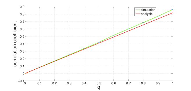
Figure 1: Degree correlation of an assortative model. Power-law degree distribution and $b=6$

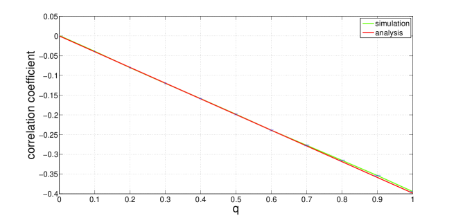
Figure 2: Degree correlation of a disassortative model. Power-law degree distribution and $b=6$

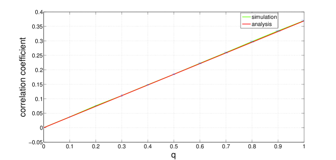
Figure 3: Degree correlation of a assortative model. Power-law degree distribution and $b=2$

For percolation analysis, we study the critical value of $\phi$. We assume that degrees are geometrically distributed. However, geometrical distributions do not satisfy Assumption 1. Assumption 1 is essential. Without this assumption, $1$ is not a fixed point and numerical calculations would fail. We can adjust the probability masses to make Assumption 1 hold. We illustrate this modification for the $b=2$ case. We start with a geometric degree distribution $(1-p)p^{k}$, where $k=0,1,\ldots$, and $p=2/3$. The corresponding ${\bf\sf E}(Z)=2$. We thus have

$$\tilde{p}_{k}=k(1-p)p^{k}/2,\quad k=0,1,\ldots$$

We move part of the probability mass from $\tilde{p}_{4}$ to $\tilde{p}_{5}$. After this modification, the distribution $\{\tilde{p}_{k}\}$ becomes

$$\tilde{p}_{k}=\left\{\begin{array}[]{ll}k(1-p)p^{k}/2&\mbox{$k\geq 0$, $k\neq 4$, $k\neq 5$;}\\ 2(1-p)p^{4}-0.0782&\mbox{if $k=4$;}\\ 5(1-p)p^{5}/2+0.0782&\mbox{if $k=5$}.\end{array}\right.$$ (43)

Let $H_{1}=\{0,1,2,3,4\}$ and $H_{2}=\{k:k\geq 5\}$. It is easy to verify that $\{\tilde{p}_{k}\}$ satisfies Assumption 1.

We study $b=2$ and $b=3$. In both cases, we study two permutations of blocks suggested in Section 4 for assortativity and disassortativity. For assortative networks, $h(i)=i$. For disassortative networks, $h(i)=b+1-i$. In the case of $b=3$, we have also studied a rotational permutation, i.e., $h(i)=((i+1)\mod b)+1$. The critical values of $\phi$ obtained using (36) are shown in Table 1. We also numerically calculate the critical values of $\phi$. In this numerical study, we gradually decrease $\phi$ until (32) fails to have a solution in the interior of $[0,1)^{b}$. From these results, we see that the critical values of $\phi$ obtained from (36) agree very well with those obtained numerically.

Finally, we study the giant component sizes of the generalized configuration models. We numerically solve (32) to obtain vector $\alpha$, and then compute $\eta$ using (25). In this study, we continue to assume that degrees are geometrically distributed as we did in the study of Table 1. The giant component sizes are shown in Figure 4. From this figure, we see that assortative networks have smaller percolation thresholds than disassortative networks. Hence, giant components emerge more easily in assortative networks. However, disassortative networks tend to have larger giant component sizes than assortative networks for large $\phi$. The effect of assortativity and disassortativity to the giant component sizes and the percolation thresholds observed in this example agrees with that observed in Newman [19]. For the effect of $q$, larger values of $q$ decrease the percolation thresholds and the giant component sizes of assortative networks. On the other hand, larger values of $q$ increase the percolation thresholds and the giant component sizes of disassortative networks.

		$q=0.2$	$q=0.5$	$q=0.8$
$b=2$, assortativity	$\phi^{\star}$	0.22662	0.19518	0.16692
	numerical	0.22662	0.19513	0.16688
$b=2$, disassortativity	$\phi^{\star}$	0.26715	0.29237	0.31231
	numerical	0.26711	0.29237	0.31229
$b=3$, assortativity	$\phi^{\star}$	0.22252	0.18095	0.14540
	numerical	0.22251	0.18092	0.14537
$b=3$, disassortativity	$\phi^{\star}$	0.27442	0.30784	0.32967
	numerical	0.27438	0.30782	0.32965
$b=3$, rotator	$\phi^{\star}$	0.26572	0.29682	0.33182
	numerical	0.26571	0.29682	0.33181

Table 1: Critical values of $\phi$.

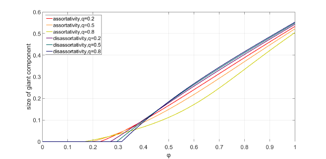
Figure 4: Size of the giant component vs. $\phi$.

7 Conclusions

In this paper we have presented an extension of the classical configuration model. Like a classical configuration model, the extended configuration model allows users to specify an arbitrary degree distribution. In addition, the model allows users to specify a positive or a negative assortative coefficient. We derived a closed form for the assortative coefficient of this model. We verified our result with simulations.

Appendix

In this appendix we prove Theorem 3. To achieve this, we need a matrix version of the mean value theorem. We state the result in the following lemma.

Lemma 1

Suppose that $x$ and $y$ are two points in $[0,1]^{b}$. Then, there exists constants $c_{i}$ in the open intervals $(\min(x_{i},y_{i}),\max(x_{i},y_{i}))$, such that

$${\mbox{\boldmath$f$}}({\mbox{\boldmath$x$}})-{\mbox{\boldmath$f$}}({\mbox{\boldmath$y$}})={\mbox{\boldmath$J$}}({\mbox{\boldmath$c$}})({\mbox{\boldmath$x$}}-{\mbox{\boldmath$y$}}),$$ (44)

where ${\mbox{\boldmath$c$}}=(c_{1},c_{2},\ldots,c_{b})$.

Proof (Lemma 1)

Suppose that $x$ and $y$ are two points in $[0,1]^{b}$. Consider

$$f_{i}({\mbox{\boldmath$x$}})-f_{i}({\mbox{\boldmath$y$}}) = \phi(bq+1-q)\left(g_{h(i)}(x_{h(i)})-g_{h(i)}(y_{h(i)})\right)$$ (45)

$$\ +\phi(1-q)\sum_{j=1,j\neq h(i)}^{b}\left(g_{j}(x_{j})-g_{j}(y_{j})\right).$$

Since function $g_{j}$ is continuous and differentiable in $(0,1)$, by the mean value theorem there is a $c_{j}$, where $\min(x_{j},y_{j})<c_{j}<\max(x_{j},y_{j})$, such that

$$g_{j}^{\prime}(c_{j})=\frac{g_{j}(x_{j})-g_{j}(y_{j})}{x_{j}-y_{j}}$$ (46)

for all $j$. Substituting (43) into (42) and expressing (42) in matrix form, we immediately prove (41).  

The proof of Theorem 3 also needs the Poincaré-Miranda Theorem, which is a gereralization of the intermediate value theorem. We quote the Poincaré-Miranda Theorem from [10]. Let $I^{b}=[0,1]^{b}$ be the $b$-dimensional cube of the Euclidean space $R^{b}$. For each $i\leq b$ denote

$$I_{i}^{-}\stackrel{{\scriptstyle\scriptstyle\rm def}}{{=}}\{{\mbox{\boldmath$x$}}\in I^{b}:x_{i}=0\},\qquad I_{i}^{+}\stackrel{{\scriptstyle\scriptstyle\rm def}}{{=}}\{{\mbox{\boldmath$x$}}\in I^{b}:x_{i}=1\}$$

the $i$-th opposite faces.

Proposition 2

(Poincaré-Miranda Theorem) Let ${\mbox{\boldmath$f$}}:I^{b}\to R^{b}$, ${\mbox{\boldmath$f$}}=(f_{1},f_{2}$, $\ldots$, $f_{b})$, be a continuous map such that for each $i\leq b$, $f_{i}(I_{i}^{-})\subset(-\infty,0]$ and $f_{i}(I_{i}^{+})\subset[0,+\infty)$. Then, there exists a point ${\mbox{\boldmath$c$}}\in I^{b}$ such that ${\mbox{\boldmath$f$}}({\mbox{\boldmath$c$}})={\mbox{\boldmath$0$}}$.

Now we prove Theorem 3.

Proof (Theorem 3)

Now we analyze the first case in Theorem 3. We have shown that fixed point $1$ is attracting. We now show that there is no other fixed point in $[0,1]^{b}$. Suppose not. Assume that there is another distinct fixed point. Denote it by $x$. From Lemma 1, we have

$${\mbox{\boldmath$1$}}-{\mbox{\boldmath$x$}}={\mbox{\boldmath$J$}}({\mbox{\boldmath$c$}})({\mbox{\boldmath$1$}}-{\mbox{\boldmath$x$}}).$$ (47)

Since $g_{i}$ is a power series with non-negative coefficients, $g_{i}$ is monotonically increasing, differentiable and $g_{i}^{\prime}$ is also increasing. Thus,

$${\mbox{\boldmath$J$}}({\mbox{\boldmath$c$}}) = \phi(bq{\mbox{\boldmath$H$}}+(1-q){\mbox{\boldmath$1$}}_{b\times b}){\mbox{\boldmath$D$}}\{g_{1}^{\prime}(c_{1}),g_{2}^{\prime}(c_{2}),\ldots,g_{b}^{\prime}(c_{b})\}$$

$$\leq \phi(bq{\mbox{\boldmath$H$}}+(1-q){\mbox{\boldmath$1$}}_{b\times b}){\mbox{\boldmath$D$}}\{g_{1}^{\prime}(1),g_{2}^{\prime}(1),\ldots,g_{b}^{\prime}(1)\}$$

$$= {\mbox{\boldmath$J$}}({\mbox{\boldmath$1$}})$$

component-wise. Inequality (45) is due to the fact that $H$, ${\mbox{\boldmath$1$}}_{b\times b}$ and the two diagonal matrices are all non-negative. Substituting the inequality above into (44), we have

$${\mbox{\boldmath$1$}}-{\mbox{\boldmath$x$}}\leq{\mbox{\boldmath$J$}}({\mbox{\boldmath$1$}})({\mbox{\boldmath$1$}}-{\mbox{\boldmath$x$}}).$$

Substituting the last inequality repeatedly into itself, we have

$${\mbox{\boldmath$1$}}-{\mbox{\boldmath$x$}}\leq{\mbox{\boldmath$J$}}({\mbox{\boldmath$1$}})^{n}({\mbox{\boldmath$1$}}-{\mbox{\boldmath$x$}})\to{\mbox{\boldmath$0$}},$$

as $n\to\infty$, since the dominant eigenvalue of ${\mbox{\boldmath$J$}}({\mbox{\boldmath$1$}})$ is strictly less than one. We thus reach a contradiction to the assumption that $x$ is distinct from $1$.

Now we consider the second case. We first show that there exists a point $x$ in $[0,1]^{b}$ such that

$${\mbox{\boldmath$x$}}-{\mbox{\boldmath$f$}}({\mbox{\boldmath$x$}})\geq{\mbox{\boldmath$0$}}.$$

Denote such a point by $\eta$. We choose

$${\mbox{\boldmath$\eta$}}={\mbox{\boldmath$1$}}-\epsilon{\mbox{\boldmath$v$}},$$ (49)

where $\epsilon$ is a small positive number and $v$ is the eigenvalue of ${\mbox{\boldmath$J$}}({\mbox{\boldmath$1$}})$ associated with the dominant eigenvalue $\phi\lambda_{1}$. For small $\epsilon$, we have

$${\mbox{\boldmath$f$}}({\mbox{\boldmath$\eta$}})={\mbox{\boldmath$f$}}({\mbox{\boldmath$1$}}-\epsilon{\mbox{\boldmath$v$}})\approx{\mbox{\boldmath$f$}}({\mbox{\boldmath$1$}})-{\mbox{\boldmath$J$}}({\mbox{\boldmath$1$}})(\epsilon{\mbox{\boldmath$v$}})={\mbox{\boldmath$1$}}-{\mbox{\boldmath$J$}}({\mbox{\boldmath$1$}})(\epsilon{\mbox{\boldmath$v$}}).$$

It follows from the above equation that

$${\mbox{\boldmath$\eta$}}-{\mbox{\boldmath$f$}}({\mbox{\boldmath$\eta$}})\approx({\mbox{\boldmath$J$}}({\mbox{\boldmath$1$}})-{\mbox{\boldmath$I$}})(\epsilon{\mbox{\boldmath$v$}}),$$ (50)

where $I$ is the $b\times b$ identity matrix. Since $v$ is an eigenvector of ${\mbox{\boldmath$J$}}({\mbox{\boldmath$1$}})$ associated with $\phi\lambda_{1}$, (47) reduces to

$${\mbox{\boldmath$\eta$}}-{\mbox{\boldmath$f$}}({\mbox{\boldmath$\eta$}})=(\phi\lambda_{1}-1)\epsilon{\mbox{\boldmath$v$}}.$$

Since $\phi\lambda_{1}>1$ and ${\mbox{\boldmath$v$}}>{\mbox{\boldmath$0$}}$ entry-wise, we have

$${\mbox{\boldmath$\eta$}}-{\mbox{\boldmath$f$}}({\mbox{\boldmath$\eta$}})>{\mbox{\boldmath$0$}}$$ (51)

for some $\epsilon>0$.

Next we shall show that (32) has another fixed point in $[0,1)^{b}$. To apply Proposition 2, we transform system (32) by changing variables. That is, for any $x_{i}\in[0,\eta_{i}]$, where $\eta_{i}$ is the $i$-th entry of $\eta$ defined in (46). We define $y_{i}=x_{i}/\eta_{i}$, for $i=1,2,\ldots,b$. Then, we define function ${\mbox{\boldmath$F$}}:[0,1]^{b}\to[0,1]^{b}$, where the $i$-th entry of $F$ is

$$F_{i}({\mbox{\boldmath$y$}})=\eta_{i}y_{i}-f_{i}(\eta_{1}y_{1},\eta_{2}y_{2},\ldots,\eta_{b}y_{b}).$$

We now show that for any ${\mbox{\boldmath$y$}}\in I_{i}^{-}$,

$$F_{i}({\mbox{\boldmath$y$}})$$

$$=-f_{i}(\eta_{1}y_{1},\eta_{2}y_{2},\ldots,\eta_{b}y_{b})$$

$$=-(1-\phi)-\phi\left((bq+1-q)g_{h(i)}(\eta_{h(i)}y_{h(i)})+(1-q)\sum_{j\neq h(i)}g_{j}(\eta_{j}y_{j})\right)$$

$$\leq 0,$$

since $g_{j}(\eta_{j}y_{j})\leq 1/b$ for all $j$. Next, consider $y$ in $I_{i}^{+}$. In this case,

$$F_{i}({\mbox{\boldmath$y$}}) = \eta_{i}-f_{i}(\eta_{1}y_{1},\ldots,\eta_{i-1}y_{i-1},\eta_{i},\eta_{i+1}y_{i+1},\ldots,\eta_{b}y_{b})$$ (52)

$$\geq \eta_{i}-f_{i}(\eta_{1},\ldots,\eta_{i-1},\eta_{i},\eta_{i+1},\ldots,\eta_{b})$$

$$\geq 0,$$ (53)

where (49) follows from the monotonicity of $g_{j}$ for all $j$, and (50) follows from (48). From Proposition 2,, ${\mbox{\boldmath$F$}}({\mbox{\boldmath$y$}})={\mbox{\boldmath$0$}}$ has a root in $[0,1]^{b}$. Equivalently, (32) has a root in $[0,1)^{b}$. We denote this root by $z$.

We now show that fixed point $z$ is attracting. From (41) since both $1$ and $z$ are fixed points, we have

$${\mbox{\boldmath$1$}}-{\mbox{\boldmath$z$}}={\mbox{\boldmath$J$}}({\mbox{\boldmath$c$}})({\mbox{\boldmath$1$}}-{\mbox{\boldmath$z$}}),$$ (54)

where $z_{i}<c_{i}<1$. From (51), the unity is an eigenvalue of ${\mbox{\boldmath$J$}}({\mbox{\boldmath$c$}})$ and ${\mbox{\boldmath$1$}}-{\mbox{\boldmath$z$}}$ is the associated eigenvector. Since ${\mbox{\boldmath$J$}}({\mbox{\boldmath$c$}})$ is a positive matrix and ${\mbox{\boldmath$1$}}-{\mbox{\boldmath$z$}}$ is a positive vector component-wise, by the Perron-Frobenius theorem, the unity is the dominant eigenvalue of ${\mbox{\boldmath$J$}}({\mbox{\boldmath$c$}})$ [14]. By the definition in (30), $g_{i}^{\prime}$ is strictly increasing for all $i$. It follows that $g_{i}^{\prime}(c_{i})>g_{i}^{\prime}(z_{i})$ and from (35) we have

$${\mbox{\boldmath$J$}}({\mbox{\boldmath$c$}}) = \phi(bq{\mbox{\boldmath$H$}}+(1-q){\mbox{\boldmath$1$}}_{b\times b}){\mbox{\boldmath$D$}}\{g_{1}^{\prime}(c_{1}),g_{2}^{\prime}(c_{2}),\ldots,g_{b}^{\prime}(c_{b})\}$$ (55)

$$> \phi(bq{\mbox{\boldmath$H$}}+(1-q){\mbox{\boldmath$1$}}_{b\times b}){\mbox{\boldmath$D$}}\{g_{1}^{\prime}(z_{1}),g_{2}^{\prime}(z_{2}),\ldots,g_{b}^{\prime}(z_{b})\}$$

$$= {\mbox{\boldmath$J$}}({\mbox{\boldmath$z$}})$$

component-wise. Recall that we assume $q<1$. With $\phi>0$, it is clear that both ${\mbox{\boldmath$J$}}({\mbox{\boldmath$c$}})$ and ${\mbox{\boldmath$J$}}({\mbox{\boldmath$z$}})$ are irreducible matrices. From Theorem 9 of [24](see also [9]), (52) implies that the spectral radius of ${\mbox{\boldmath$J$}}({\mbox{\boldmath$z$}})$ is strictly less than that of ${\mbox{\boldmath$J$}}({\mbox{\boldmath$c$}})$. This implies that $z$ is an attracting fixed point.

References

- (1) Barabási, A.-L. and Albert, R. (1999). Emergence of scaling in random networks. Science 286, 509–512.
- (2) Bender, E. A. and Canfield, E. R. (1978). The asymptotic number of labelled graphs with given degree sequences. J. Comb. Theory Series A 24, 296–307.
- (3) Boguna, M., Pastor-Satorras, R. and Vespignani, A. (2003). Absence of epidemic threshold in scale-free networks with degree correlations. Physical Review Letters 90,.
- (4) Bratley, P., Fox, B. L. and Schrage, L. E. (1987). A Guide to Simulation 2 ed. Springer-Verlag, New York.
- (5) Cardy, J. and Grassberger, P. (1985). Epidemic models and percolation. J. Phys. A: Math. Gen. 18,.
- (6) Cohen, R., Erez, K., ben Avraham, D. and Havlin, S. (2000). Resilence of the internet to random breakdowns. Phys. Rev. Lett. 85, 4626–4628.
- (7) Eguíluz, V. M. and Klemm, K. (2002). Epidemic threshold in structured scale-free networks. Physical Review Letters 89,.
- (8) Erdős and Rényi (1959). On random graphs. Publicationes Mathematicicae 6, 290–297.
- (9) Guiver, C. (2018). On the strict monotonicity of spectral radii for classes of bounded positive linear operators. Positivity 22, 1173–1190.
- (10) Kulpa, W. (1997). The Poincaré-Miranda theorem. The American Mathematical Monthly 104(6), 545–550.
- (11) Lancaster, P. and Tismenetsky, M. (1985). The Theory of Matrices. Academic Press, New York.
- (12) Litvak, D. N. and van der Hofstad, R. Degree-degree correlations in random graphs with heavy-tailed degrees October 2012.
- (13) Marshall, A., Olkin, I. and Arnold, B. C. (2011). Inequalities: Theory of Majorization and Its Applications. Springer, New York.
- (14) Meyer, C. (2000). Matrix analysis and applied linear algebra. SIAM, Philadelphia, USA.
- (15) Molloy, M. and Reed, B. (1995). A critical point for random graphs with a given degree sequence. Random Struct. Alg. 6, 161–179.
- (16) Moore, C. and Newman, M. (2000). Epidemics and percolation in small-world networks. Phys. Rev. E 61, 5678.
- (17) Moreno, Y., Gómez, J. B. and Pacheco, A. F. (2003). Epidemic incidence in correlated complex networks. Physical Review E 68, 035103.
- (18) ná, M. B. and Pastor-Satorras, R. (2002). Epidemic spreading in correlated complex networks. Physical Review E 66, 047104.
- (19) Newman, M. (2002). Assortative mixing in networks. Physical Review Letters 89, 208701.
- (20) Newman, M. (2003). Mixing patterns on networks. Phys. Rev. E 67, 026126.
- (21) Newman, M. (2010). Networks: An Introduction. Oxford University Press, New York.
- (22) Nikoloski, Z., Deo, N. and Kucera, L. (2005). Degree-correlation of a scale-free random graph process. In Proc. Discrete Mathematics and Theoretical Computer Science. vol. AE. pp. 239–244.
- (23) Ramezanpour, A., Karimipour, V. and Mashaghi, A. (2005). Generating correlated networks from uncorrelated ones. Physical Review E 67, 046107.
- (24) Rheinboldt, W. and Vandergraft, J. (1973). A simple approach to the perron–frobenius theory for positive operators on general partially-ordered finite-dimensional linear spaces. Math. Comput. 27, 139–145.
- (25) Sander, L., Warren, C., Sokolov, I., Simon, C. and Koopman, J. (2002). Percolation on heterogeneous networks as a model for epidemics. Mathematical Biosciences 80, 293–305.
- (26) Schläpfer, M. and Buzna, L. (2012). Decelerated spreading in degree-correlated networks. Physical Review E 85, 015101.
- (27) Schwartz, N., Cohen, R., ben Avraham, D., Barabasi, A.-L. and Havlin, S. (2002). Percolation in directed scale-free networks. Phys. Rev. E. 66, 015104.
- (28) Vázquez, A. and Moreno, Y. (2003). Resilence to damage of graphs with degree correlations. Physical Review E 67, 015101.
- (29) Watts, D. J. and Strogatz, S. H. (1998). Collective dynamics of ’small-world’ networks. Nature 393, 440–442.
- (30) Xulvi-Brunet, R. and Sokolov, I. M. (2005). Changing correlations in networks: assortativity and dissortativity. Acta Physica Polonica B 36, 1431–1455.
- (31) Zhou, J., Xu, X., Zhang, J., Sun, J., Small, M. and Lu, J.-A. (2008). Generating an assortative network with a given degree distribution. Intern. J. of Bifuration and Chaos 18, 3495– 3502.