Evolution of the magnetic and polaronic order of $\rm{Pr_{1/2}Ca_{1/2}MnO_{3}}$ following an ultrashort light pulse.

Abstract

The dynamics of electrons, spins and phonons induced by optical femtosecond pulses has been simulated for the polaronic crystal $\rm{Pr_{1/2}Ca_{1/2}MnO_{3}}$. The model used for the simulation has been derived from first-principles calculations. The simulations reproduce the experimentally observed melting of charge/orbital order with increasing fluence. The loss of charge order in the high-fluence regime induces a transition to a ferromagnetic metal. At low fluence, the dynamics is deterministic and coherent phonons are created by the repopulation of electronic orbitals, which are strongly coupled to the phonon degrees of freedom. In contrast to the low-fluence regime, the magnetic transitions occurring at higher fluence can be attributed to a quasi-thermal transition of a cold-plasma-like state with hot electrons and cold phonons and spins. The findings can be rationalized in a more complete picture of the electronic structure that goes beyond the simple ionic picture of charge order.

I Introduction

Unlike traditional spectroscopy, ultrafast pump-probe spectroscopy is a powerful tool to dynamically track the interactions in a strongly correlated system. Specifically, manganites are a suitable model system, because different types of correlations between electrons, spins and phonons have similar strength. A number of different electronic ground states can be realized just by changing temperature or doping. In these materials, high-resolution ultrafast pump-probe spectroscopy experiments have unraveled interesting physical effects, such as photo-induced phase transitions Ren et al. (2008); Matsubara et al. (2007); Ogasawara et al. (2003) and transient "hidden" phases Ichikawa et al. (2011).

In manganite perovskites, a growing number of ultrafast experiments provide access to the dynamics on different time scales from femto- to nanoseconds. The dynamics depends on the phase of the selected manganite as well as on the photon energy and intensity of the pump pulse. In $\rm{GdSrMnO_{3}}$ close to half doping, a photo-induced transition from a charge-order phase to a ferromagnetic metallic phase within 200 fs has been observedMatsubara et al. (2007). An ultrafast metal-insulator transition has been induced in $\rm{Pr_{0.7}Ca_{0.3}MnO_{3}}$ by selectively exciting phonon modes at 625 cm^-1 Rini et al. (2007). On shorter timescales, coherent oscillations in the sample resistance in the insulator-to-metal dynamics with 30 THz are interpreted as orbital waves.Polli et al. (2007) Several ultrafast optical-pump terahertz-probe studies in manganites focused on probing the nature of the quasi particles and their dynamics within a given phase Polli et al. (2007); Rini et al. (2007); Raiser et al. (2017).

Optical pump-probe experiments suggest a two-component relaxation process in $\rm{Nd_{0.5}Sr_{0.5}MnO_{3}}$Prasankumar et al. (2007) and $\rm{La_{0.7}Ca_{0.3}MnO_{3}}$ Averitt et al. (2001); Wu et al. (2009); Bielecki et al. (2010). In the paramagnetic insulating phase of $\rm{La_{0.7}Ca_{0.3}MnO_{3}}$, the fast component ${<}1$ ps involves thermalization of electronic subsystem and its energy redistribution with the lattice subsystem. The slower component on the 20-200 ps timescale, with a $\rm{T_{c}}$-dependent lifetime, is attributed to the spin-lattice relaxation Ogasawara et al. (2003); Wu et al. (2009); Bielecki et al. (2010).

Recently, long-lived polaron-type optical excitations with lifetime of 1-2 ns are observed in the charge-ordered phase of $\rm{Pr_{0.7}Ca_{0.3}MnO_{3}}$ Raiser et al. (2017). Another long-lived intermediate state, with a mixture of ferromagnetic metallic and charge-ordered nanoscale domains, is observed in $\rm{La_{0.325}Pr_{0.3}Ca_{0.375}MnO_{3}}$ Lin et al. (2018).

Depending on the phase and excitation intensity, coherent acoustic phonons as well as oscillating strain waves are observed on time scales of several 10 ps Thomsen et al. (1984); Zeiger et al. (1992); for manganites see Jang et al. (2010).

The goal of this work is to augment previous experimental studies with a detailed description of the microscopic processes occurring during the first few picoseconds. For this purpose, we perform simulations, that are verified by comparing our findings with experimental observations. The work presented here is parameter free in the sense that the model parameters have been extracted from first-principles calculationsSotoudeh et al. (2017).

We simulate the photo-excitation of $\rm{Pr_{\nicefrac{{1}}{{2}}}Ca_{\nicefrac{{1}}{{2}}}MnO_{3}}$ by a femto-second light pulse and the subsequent relaxation of the magnetic and polaronic microstructure for the first few picoseconds. Ehrenfest dynamicsTully (1998) is adopted to propagate wave functions, spins and atoms. Peierls substitution has been employed to incorporate the external light pulse. A systematic study is performed to investigate the relaxation process by varying the intensity of the light pulse.

The paper is organized as follows: The methods of the paper are covered in section II: The tight-binding model used for the electron, spin and phonon degrees of freedom is described first, followed by the dynamical equations of motion, the treatment of the optical excitation and quantities used in the analysis. In section III, we revisit the ground state of $\rm{Pr_{\nicefrac{{1}}{{2}}}Ca_{\nicefrac{{1}}{{2}}}MnO_{3}}$, which experiences the optical excitation. Thereafter, we describe in section IV the results of our simulations and discuss the underlying mechanisms. Finally we summarize the findings in section V.

II Methods

II.1 Tight-Binding model

To investigate the electronic, atomic and magnetic microstructure of manganites, we employ a tight-binding modelDagotto et al. (2001); Hotta and Dagotto (2002); Hotta (2006). The selection of energy terms and the parameter values have been extracted from the first-principles calculationsSotoudeh et al. (2017).

The model describes the correlations between electron, spin and phonon degrees of freedom. The explicit electronic degrees of freedom describe the Mn-d-electrons with $\rm{e_{g}}$-character. The spin degrees of freedom describe the three majority-spin d-orbitals of each Mn ion with $\rm{t_{2g}}$ character. The phonon degrees of freedom are two Jahn-Teller active vibration modes and one breathing mode of each MnO₆ octahedron. In addition, we allow for a global expansion of the lattice.

The potential-energy functional of the system is

$$E_{pot}=E_{e}+E_{S}+E_{ph}+E_{e-ph}+E_{e-S}\;,$$ (1)

where the $E_{e}$, $E_{S}$ and $E_{ph}$ are the energies of the isolated electronic, spin and phonon subsystems, respectively. $E_{e-ph}$ is the electron-phonon coupling of Mn-$\rm{e_{g}}$ electrons with the Jahn-Teller active modes as well as with the breathing mode of the MnO₆ octahedra. $E_{e-S}$ is Hund’s coupling between the $\rm{e_{g}}$ electrons and the spins of the Mn-$\rm{t_{2g}}$ electrons.

Our model avoids the common infinite-Hund’s-coupling limit,Müller-Hartmann and Dagotto (1996) and uses a more realistic description with explicit minority-spin electrons and a fully non-collinear treatment of the electron spin. Furthermore, we include the strong cooperativity of Jahn-Teller distortions and octahedral breathing modes by expressing them in terms of the explicit oxygen positions, which are shared each by two adjacent MnO₆ octahedra.

The Mn $\rm{e_{g}}$ electrons are described by a Slater determinant formed by the one-particle wave functions $|\psi_{n}\rangle$. The latter are expressed as superposition of local orbitals $|\chi_{\sigma,\alpha,R}\rangle$ with complex-valued coefficients $\psi_{\sigma,\alpha,R,n}$

$$|\psi_{n}\rangle=\sum\limits_{\sigma,\alpha,R}|\chi_{\sigma,\alpha,R}\rangle\psi_{\sigma,\alpha,R,n}\;.$$ (2)

The local orbital $|\chi_{\sigma,\alpha,R}\rangle$ is a spin-orbital with $\rm{e_{g}}$ character at the Mn site $R$. It is a spin eigenstate with spin $\sigma\in\{\uparrow,\downarrow\}$ and spatial orbital character $\alpha$ $\in$ $\{a,b\}$ (where $a{=}d_{x^{2}-y^{2}}$ and $b{=}d_{3z^{2}-r^{2}}$) Sotoudeh et al. (2017). The wavefunctions are Pauli spinor wavefunctions that account for the non-collinear nature of the magnetization.

The three majority-spin $\rm{t_{2g}}$ electrons of a Mn site with site index $R$ are described by a spin vector $\vec{S}_{R}$ Sotoudeh et al. (2017). The two Jahn-Teller active phonon modes $Q_{2,R}$ and $Q_{3,R}$ for each $\rm{MnO_{6}}$ octahedron as well as the breathing mode $Q_{1,R}$ are expressed by the displacements of oxygen ions along the Mn-O-Mn bridge using Eq. 22 of Sotoudeh et al. (2017).

II.2 Dynamics

The dynamics of the optical excitation and its relaxation processes are described by Ehrenfest dynamicsMcLachlan (1964); Tully (1998): That is, the electrons evolve under the time-dependent Schrödinger equation, while the atoms are treated as classical particles and obey Newton’s equations of motion.

$$i\hbar\partial_{t}\psi_{\sigma,\alpha,R,n} = \frac{\partial E_{pot}}{\partial\psi^{*}_{\sigma,\alpha,R,n}}$$ (3)

$$\partial_{t}S_{j,R} = \frac{2m_{S}}{\hbar}\vec{B}_{R}\times\vec{S}_{R}$$ (4)

$$M_{O}\partial^{2}_{t}R_{j} = -\frac{\partial E_{pot}}{\partial R_{j}}$$ (5)

$R_{j}$ are the structural degrees of freedom of the oxygen ions and $M_{O}$ is their mass. $m_{S}$ is the absolute value of the magnetic moment of the $\rm{t_{2g}}$-spins and the quasi-magnetic field $\vec{B}_{R}$ is

$$B_{j,R}=\frac{3\hbar}{2m_{S}}\frac{\partial E}{\partial S_{j,R}}$$ (6)

Further details are given in appendices A and B. We also allowed for a strain dynamics, which does not have notable consequences on the results presented here. For the sake of completeness, it is described in appendix C.

II.3 Light Pulse

The light pulse is described by a spatially homogeneous, but time-dependent electromagnetic field (see appendix D)

$$\vec{E}(t)=\vec{e}_{A}\omega{\rm Im}\left(A_{0}^{*}{\rm e}^{i\omega t)}\right)g(t)\;,$$ (7)

where $A_{0}$ is the amplitude of the vector potential and $\hbar\omega$ is the photon energy. $c$ is the speed of light. The polarization of the electric field and of the vector potential is the unit vector $\vec{e}_{A}$.

The temporal profile of the laser pulse is described by a Gaussian

$$g(t)=\frac{1}{\sqrt[4]{\pi c_{w}^{2}}}{\rm e}^{-\frac{t^{2}}{2c_{w}^{2}}}$$ (8)

The intensity, which is proportional to $|g(t)|^{2}$, has the full-width-at-half-maximum (FWHM) of $2c_{w}\sqrt{\ln 2}$.

The light pulse is implemented with the Peierls-substitution method Peierls (1933); Hofstadter (1976). Details are given in Appendix D.

II.4 Parameters of the simulation

Tab. 1 summarizes the relevant parameters used in this paper.

Table 1: Simulation parameters. For explanation, see text.

k-grid	$1{\times}1{\times}1$
supercell	$N_{x}{\times}N_{y}{\times}N_{z}{=}8{\times}8{\times}4$
Mn sites per unit cell	$N_{Mn}=256$
O sites per unit cell	$N_{O}=768$
Mn-Mn spacing	$d_{Mn-Mn}=3.84$ Å
time step	$\Delta_{t}{=}0.040(4\pi\epsilon_{0})^{2}\hbar^{3}/(m_{e}e^{4})$
	$=0.97\times 10^{-18}$ s
oxygen mass	$M_{O}=15.998$ u
fictitious cell mass	$M_{g}{=}8.0{\times}10^{10}$ me
photon energy	$\hbar\omega=1.17$ eV
pulse length (FWHM)	$2\sqrt{\ln 2}c_{w}=100~{}{\rm fs}$
polarization	$\vec{e}_{A}=(\vec{e}_{x}+\vec{e}_{y})/\sqrt{2}$
initial tetragonal distortion	$g_{x}=g_{y}=1.0388$, $g_{z}=1.0077$

We use a Cartesian coordinate system with the coordinate axes $\vec{e}_{x}$, $\vec{e}_{y}$ and $\vec{e}_{z}$ pointing along the Mn-Mn nearest-neighbor distances. The vectors $\vec{e}_{j}$ are defined with length 1.

The Mn-Mn nearest-neighbor vectors are $g_{x}d_{Mn-Mn}\vec{e}_{x}$, $g_{y}d_{Mn-Mn}\vec{e}_{y}$, and $g_{z}d_{Mn-Mn}\vec{e}_{z}$ with $d_{Mn-Mn}$ from Tab. 1 and scale factors $g_{x}$, $g_{y}$ and $g_{z}$. With $N_{x}$, $N_{y}$ and $N_{z}$, we denote the number of Mn sites in each of the three spatial directions in the supercell used in the calculation.

To describe perovskites, one usually refers to the lattice vectors of Pbnm unit cell, an non-standard setting of space group 62. The lattice vectors $\vec{a}$, $\vec{b}$ and $\vec{c}$ of the Pbnm unit cell are

$$\vec{a} = \left(g_{x}\vec{e}_{x}-g_{y}\vec{e}_{y}\right)d_{Mn-Mn}$$

$$\vec{b} = \left(g_{x}\vec{e}_{x}+g_{y}\vec{e}_{y}\right)d_{Mn-Mn}$$

$$\vec{c} = 2g_{z}\vec{e}_{z}d_{Mn-Mn}$$ (9)

The pulse length has been chosen consistent with the laser pulses used in ultrafast pump-probe experimentsRaiser et al. (2017).

II.5 Diffraction patterns

In order to link our results with diffraction experiments, we inspect the intensities of diffraction for charges, orbitals and spins.

The intensity of diffraction of an observable $\hat{X}$, such as number of electrons, orbital occupations, or spins, with density $x(\vec{r})$ isFeil (1977)

$$I_{X}(\vec{q}):=I_{X,0}(\vec{q})\left|\int_{V}d^{3}r\;x(\vec{r}){\rm e}^{-i\vec{q}\vec{r}}\right|^{2}$$ (10)

where the integration is performed over the illuminated sample volume $V$. $I_{X,0}(\vec{q})$ is the intensity of diffraction of a point scatterer $x(\vec{r})=X\delta(\vec{r})$.

For a periodic lattice of atom-centered distributions $x(\vec{r})=\sum_{R,\vec{t}}x_{R}(\vec{r}-\vec{R}_{R}-\vec{t})$, the intensity of diffraction is

$$I_{X}(\vec{q}) = I_{X,0}(\vec{q})N_{\in V}\Omega_{G}\sum_{G}\delta(\vec{q}-\vec{G})C_{X}(\vec{G})$$ (11)

with the correlation functionHotta and Dagotto (2000)

$$C_{X}(\vec{G})=\frac{1}{N}\biggl{|}\sum_{R=1}^{N}{\rm e}^{-i\vec{G}\vec{R}_{R}}X_{R}(\vec{G})\biggr{|}^{2}$$ (12)

The distributions $x_{R}(\vec{r})$ are placed at the lattice sites $\vec{R}_{R}+\vec{t}$, where $\vec{R}_{R}$ is the position of an atom inside the first unit cell and $\vec{t}$ is the lattice translation vector of a specific unit cell. $N$ is the number of atoms in the unit cell, $\Omega_{T}$ is the unit-cell volume, $\Omega_{G}=(2\pi)^{3}/\Omega_{T}$ is the unit-cell volume of the reciprocal lattice and $\vec{G}$ are the corresponding general reciprocal-lattice vectors. $N_{\in V}$ is the number of sites in the illuminated region. $X_{R}(\vec{q}):=\int d^{3}r\;x_{R}(\vec{r}){\rm e}^{-i\vec{q}\vec{r}}$ is the form factor of $x_{R}$. Note that the correlation function is meaningful only at the reciprocal lattice vectors $\vec{G}$.

Specifically, we address the following diffraction patterns:

• The charge-order correlation functionHotta and Dagotto (2000)

  $$C_{Q}(\vec{G}) := \frac{1}{N}\biggl{|}\sum_{R=1}^{N}{\rm e}^{i\vec{G}\vec{R}_{R}}\Big{(}n_{R}-\langle{n}\rangle\Big{)}\biggr{|}^{2}$$ (13)

  probes the deviation of the electron density from its mean value, i.e $X_{R}=n_{R}-\langle{n}\rangle$, where $n_{R}=\sum_{\alpha,\sigma}\rho_{\sigma,\alpha,R,\sigma,\alpha,R}$ is the number of $\rm{e_{g}}$-electrons on Mn-site $R$ and $\langle{n}\rangle=1-x$ with the doping $x=\frac{1}{2}$ is the average number of electrons on Mn sites. The one-particle-reduced density matrix

  $$\rho_{\sigma,\alpha,R,\sigma^{\prime},\alpha^{\prime},R^{\prime}}=:\sum_{n}f_{n}\psi_{\sigma,\alpha,R,n}\psi^{*}_{\sigma^{\prime},\alpha^{\prime},R^{\prime},n}$$ (14)

  is given by the wave-function coefficients $\psi_{\sigma,\alpha,R,n}$ and the occupations $f_{n}$.

• The orbital-order correlation function

  $$C_{O}(\vec{G}) {:=} \frac{1}{N}\biggl{|}\sum_{R=1}^{N}{\rm e}^{i\vec{G}\vec{R}_{R}}\left(n_{x,R}-n_{y,R}\right)\biggr{|}^{2}$$ (15)

  probes difference between the orbital occupations $X_{j,R}=n_{x,R}-n_{y,R}$, where

  $$n_{j,R}{=}\sum_{\alpha,\beta}\langle\theta_{j}|\chi_{\alpha}\rangle\biggl{(}\sum_{\sigma}\rho_{\sigma,\alpha,R,\sigma,\beta,R}\biggr{)}\langle\chi_{\beta}|\theta_{j}\rangle$$ (16)

  are calculated for the set of orthonormal orbitals $|\theta_{j}\rangle$ with $j\in\{x,y\}$, which are nearly axial in the $x$, respectively the $y$ direction. These orbitals are defined in terms of the original basis states $|d_{x^{2}-y^{2}}\rangle$ and $|d_{3z^{2}-r^{2}}\rangle$ as

  $$|\theta_{x}\rangle := \left(|d_{3z^{2}-r^{2}}\rangle-|d_{x^{2}-y^{2}}\rangle\right)\frac{1}{\sqrt{2}}$$ (17)

  and

  $$|\theta_{y}\rangle := -\left(|d_{3z^{2}-r^{2}}\rangle+|d_{x^{2}-y^{2}}\rangle\right)\frac{1}{\sqrt{2}}\;.$$ (18)

  We skip spin and site indices of the Wannier-like orbitals for scalar products, where they are identical.

• The spin-correlation functionHotta and Dagotto (2000)

  $$C_{S}(\vec{G}) := \frac{1}{N}\left|\sum_{R=1}^{N}{\rm{e}}^{i\vec{G}\vec{R}_{R}}(\vec{S}_{R}+\vec{s}_{R})\right|^{2}$$ (19)

  probes the total spin $\vec{X}_{R}=\vec{S}_{R}+\vec{s}_{R}$ of the Mn-sites, where $\vec{S}_{R}$ is the spin of the $\rm{t_{2g}}$ electrons and $\vec{s}_{R}$ is the spin of the $\rm{e_{g}}$ electrons at Mn-site $R$.

In order to account for the blurring of the diffraction peaks due to fluctuations, we included for the time-dependent spin correlation functions, in Figs 13, 19 and 23, the contribution from a $(3\times 3\times 3)$ set of reciprocal lattice vectors of the super cell centered at the specified reciprocal lattice vector.

III Equilibrium

Before investigating the optically-induced dynamics, let us remind of the salient features of the spin, charge, orbital, and lattice order of $\rm{Pr_{\nicefrac{{1}}{{2}}}Ca_{\nicefrac{{1}}{{2}}}MnO_{3}}$ in equilibrium. The low-temperature phase serves as initial state for the excitation and it determines the time-evolution of the system.

$\rm{Pr_{x}Ca_{1-x}MnO_{3}}$ has a perovskite lattice formed by a network of corner-sharing MnO₆ octahedra. Large cations such as Ca²⁺ and Pr³⁺ fill the voids in between the octahedra. The octahedral network distorts to optimize the Coulomb energy between the ions, which results in a characteristic pattern of the octahedral tilts. This tilt pattern fits into the orthorhombic Pbnm unit cell, which holds four octahedra.

The Mn-ions occur in the formal Mn⁴⁺ and Mn³⁺ oxidation states, with spin-aligned d-electrons on each Mn site. The additional electron of Mn³⁺ produces a Jahn-Teller distortion, which is highly cooperative.

At half doping, $\rm{Pr_{x}Ca_{1-x}MnO_{3}}$ has a low-temperature phase, which is described as charge and orbital ordered.Wollan and Koehler (1955); Goodenough (1955); Jirak et al. (1985) The low-temperature phase of $\rm{Pr_{\nicefrac{{1}}{{2}}}Ca_{\nicefrac{{1}}{{2}}}MnO_{3}}$ is shown schematically in Fig. 1. It has a CE-type antiferromagnetic order exhibiting ferromagnetic zig-zag chains in the ab-plane, which proceed along the b-direction. These zig-zag chains are antiferromagnetically coupled among each other. Along the zig-zag chain, we can distinguish alternating central and corner sites. The central sites are described formally as Mn³⁺ ions and exhibit Jahn-Teller distortion, while the corner sites are formally Mn⁴⁺ ions with a negligible Jahn-Teller distortion.

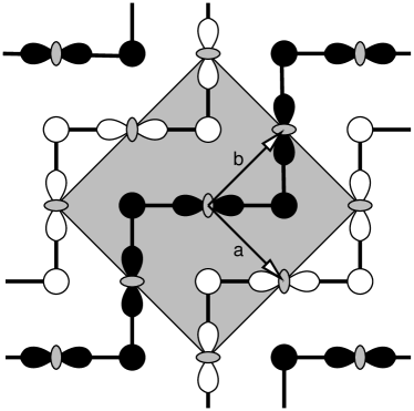
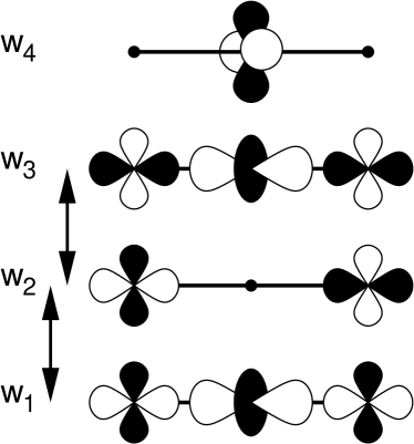
Figure 1: Left: CE-type magnetic order and orbital order in the ab-plane of the ground state of $\rm{Pr_{\nicefrac{{1}}{{2}}}Ca_{\nicefrac{{1}}{{2}}}MnO_{3}}$. Black and white symbols indicate up- and down-spins. The orbital-polarized central orbitals are indicated by a $d_{3z^{2}-r^{2}}$ orbital symbol in the corresponding direction. The corner sites have no orbital polarization and are indicated by circles. The gray square indicates the magnetic unit cell of the material in the ab-plane. Also shown are the lattice vectors $a$ and $b$ of the orthorhombic Pbnm unit cell. Right: Wannier-like orbitals along a trimer of the zig-zag chains of the CE-type magnetic structure. The sign of the orbital-lobes are indicated by black and white. The Wannier-like orbitals are orthogonal within and between trimers. The arrows connect orbitals with dipole-allowed transitions. Transitions between all other orbital pairs within and between trimers are dipole forbidden. The orbital $|w_{1}\rangle$ in the majority-spin direction is filled. The optical excitation lifts electrons from $|w_{1}\rangle$ to $|w_{2}\rangle$ in the majority-spin direction.

Table 2: Typical diffraction patterns. The diffraction spots are shown for various spin orders according to the notation of WollanWollan and Koehler (1955) as well as for charge and orbital diffraction of the CE-type low-temperature structure of $\rm{Pr_{\nicefrac{{1}}{{2}}}Ca_{\nicefrac{{1}}{{2}}}MnO_{3}}$. $(h,k,l)$ are the relative coordinates in the reciprocal lattice of the orthorhombic Pbnm setting. $h,k,l$ are integer unless mentioned otherwise. (color online)

spin	$h+k$		$l$
B-type	even integer		even integer
A-type	even integer		odd integer
C-type	odd integer		even integer
G-type	odd integer		odd integer
CE-type	$h$	$k$	$l$
spin	half-integer	half-integer	odd integer
	not integer	or integer
charge	h+k=odd integer		even integer
orbital	integer	half-integer	even integer
		not integer

III.0.1 Diffraction patterns

A transition at 250 K is attributed to the emergence of charge and/or orbital orderJirak et al. (1985) from a disordered polaron distribution at higher temperatures. The charge and orbital order has been explored experimentally by X-ray diffraction of the Mn-K-edgeZimmermann et al. (2001).

The diffraction patterns for the low-temperature phase are listed under the header CE-type in Tab. 2. The diffraction peaks are quoted as relative coordinates $(h,k,l)$ of the reciprocal lattice vectors in the setting of the orthorhombic (Pbnm) crystal structure obtained at room temperature.

Zimmermann et al.Zimmermann et al. (2001) exploited that the diffraction spots of charge and orbital order can be distinguished when scanning $(h,k,l)=(0,k,0)$ along the b-direction, the direction of the zig-zag chain. The dominant peaks of the Mn-K-edge with even integer $k$ are due to the pseudo-cubic atomic lattice of Mn-sites. The charge order introduces additional diffraction peaks at odd-integer $k$, and the orbital order produces diffraction spots at half-integer (but not integer) values of $k$, as shown in Fig. 2 and listed in Tab. 2.

At 175 K, $\rm{Pr_{\nicefrac{{1}}{{2}}}Ca_{\nicefrac{{1}}{{2}}}MnO_{3}}$ undergoes a Néel transition. Neutron-diffraction studiesJirak et al. (1985) identify the magnetic lines characteristic for the CE-type spin order for $\rm{Pr_{\nicefrac{{1}}{{2}}}Ca_{\nicefrac{{1}}{{2}}}MnO_{3}}$.

Our simulations reproduce the diffraction patterns due to charge, orbital, and spin order for the CE-type ground state as shown in Fig. 2.

The diffraction spots of other magnetic orders listed in Tab. 2 will be used to characterize the evolution of the magnetic order following the light pulse: B-type refers to a pure ferromagnet, A-type refers to ferromagnetic planes that are stacked antiferromagnetically in c-direction, C-type refers to ferromagnetic Mn-lines running along the c-direction, which are antiferromagnetically aligned with respect to neighboring strands. In a G-type antiferromagnet, the Mn-sites are antiferromagnetic with respect to all their neighbors. The magnetic orders can also be described by their wave vector of the magnetization. Expressed by the pseudo-cubic lattice formed by the Mn-sites, the B-type order refers to $\vec{k}=\frac{\pi}{d_{Mn-Mn}}(0,0,0)$, A-type refers to $\vec{k}=\frac{\pi}{d_{Mn-Mn}}(0,0,1)$ C-type refers to $\vec{k}=\frac{\pi}{d_{Mn-Mn}}(1,1,0)$ and G-type refers to $\vec{k}=\frac{\pi}{d_{Mn-Mn}}(1,1,1)$.

Figure 2: Diffraction patterns for charge-order (left), orbital order (middle) and spin order (right) of the CE-type low-temperature phase of $\rm{Pr_{\nicefrac{{1}}{{2}}}Ca_{\nicefrac{{1}}{{2}}}MnO_{3}}$. The a-axis points right, the b-axis towards the back and the c-axis up. The small white spheres indicate points with integer $h,k,l$ in the Pbnm setting. Reciprocal space is shown for $h,k,l\in[-1.25,1.25]$. (color online)

III.0.2 Charge order, orbital order and Jahn-Teller distortions

The pattern of Jahn-Teller distortions in Fig. 1 has been attributed to checkerboard-like charge order in the ab-plane with Mn³⁺ ions at the central sites of each segment and Mn⁴⁺ ions at the corner sites of the zig-zag chains.Goodenough (1955)

More recently, this picture of charge order has been challenged: Rather than deducing the charge state from the pattern of Jahn-Teller distortions, experimental techniques such as core level spectroscopy, (XANES, ELNES) and neutron diffraction measurements of the magnetic moments provide a more direct access to the charge on the ions. These experiments rule out a fully ionic picture and indicate the absence of a considerable charge disproportionationJirak et al. (1985); García et al. (2001); Grenier et al. (2004); Jooss et al. (2007); Mierwaldt et al. (2014)

This seeming contradiction between atomic structure and charge distribution can be reconciled by considering orbital polarization.Sotoudeh et al. (2017) A Mn-ion has a complete orbital polarization, when only one of the two spatial $\rm{e_{g}}$ orbitals is occupied, while the other is empty. Hereby, the shape and spin orientation of the occupied orbital is not relevant. When both spatial $\rm{e_{g}}$ orbitals are equally occupied, the atom lacks orbital polarization.

To quantify the orbital polarization at site $R$, we determine the difference $|f^{orb}_{1,R}-f^{orb}_{2,R}|$ of the orbital occupations $f^{orb}_{\alpha,R}$, which are the eigenvalues of the spin-averaged local density matrix $\bm{\rho}^{orb}_{R}$ with matrix elements

$$\rho^{orb}_{\alpha,\beta,R}:=\sum_{\sigma}\rho_{\sigma,\alpha,R,\sigma,\beta,R}\;.$$ (20)

The orbital polarization $P_{O}$ is defined as

$$P_{O} := |f^{orb}_{1,R}-f^{orb}_{2,R}|$$ (21)

$$= \sqrt{\Bigl{(}\rho^{orb}_{a,a,R}-\rho^{orb}_{b,b,R}\Bigr{)}^{2}+4\Bigl{|}\rho^{orb}_{a,b,R}\Bigr{|}^{2}}$$

where $a$ and $b$ denote the two Mn $\rm{e_{g}}$ orbitals.

Orbital polarization can be recognized indirectly via the resulting Jahn-Teller distortions. Mn-ions without orbital polarization do not exhibit a Jahn-Teller distortion, irrespective of the number of electrons in the $\rm{e_{g}}$ shell. Hence, there is a direct link between Jahn-Teller distortions and orbital polarization. The connection to the charge order is, however, indirect. It is present only in the case of complete orbital polarization. This assumption is violated in $\rm{Pr_{\nicefrac{{1}}{{2}}}Ca_{\nicefrac{{1}}{{2}}}MnO_{3}}$Sotoudeh et al. (2017). The Jahn-Teller distortions of the corner sites are small, not because of their charge, but because of their lack of orbital polarization. The orbital polarization of the corner sites is small because Wannier-like orbitals from two segments of the zig-zag chain contribute equally to the two $\rm{e_{g}}$ orbitals.Sotoudeh et al. (2017)

As shown earlierSotoudeh et al. (2017), the electronic structure of the low-temperature phase of $\rm{Pr_{\nicefrac{{1}}{{2}}}Ca_{\nicefrac{{1}}{{2}}}MnO_{3}}$ can be rationalized using a specific set of Wannier-like states formed from the Mn $\rm{e_{g}}$ orbitals. These states, shown in Fig. 1, are localized on specific segments of the zig-zag chains, which we denote, in the following, as trimers. The Wannier-like states are constructed as orthonormal eigenstates of a pseudo symmetry of a trimer, namely three orthogonal mirror planes through the central Mn-ion of a trimer. The functional form of the Wannier-like orbitals has been given in an earlier publicationSotoudeh et al. (2017). The requirements given above determine the Wannier-like orbitals up to a single parameter, which governs the charge disproportionation between central and corner sites. With a suitable choice of this parameter, the first Wannier-like state $|w_{1}\rangle$ describes the occupied states almost perfectly. This can be seen in Fig. 3, which shows that the occupied portion of the density of states can be attributed almost exclusively to $|w_{1}\rangle$. To be specific, the one-particle-reduced density matrix of the $\rm{e_{g}}$ states is well described by

$$\rho_{\sigma,\alpha,R,\sigma^{\prime},\beta,R^{\prime}} = \sum_{m}\langle\chi_{\sigma,\alpha,R}|w_{\sigma_{m},1,m}\rangle\delta_{\sigma,\sigma_{m}}\delta_{\sigma^{\prime},\sigma_{m}}$$ (22)

$$\times\langle{w}_{\sigma_{m},1,m}|\chi_{\sigma^{\prime},\beta,R^{\prime}}\rangle$$

where $|w_{\sigma,\alpha,m}\rangle$ is a Wannier-like orbital with spin $\sigma$, spatial type $j$ with $j=\{1,2,3,4\}$ according to Fig. 1 and the index $m$ specifying a particular trimer. $\sigma_{m}$ denotes the majority-spin direction of the trimer with index $m$.

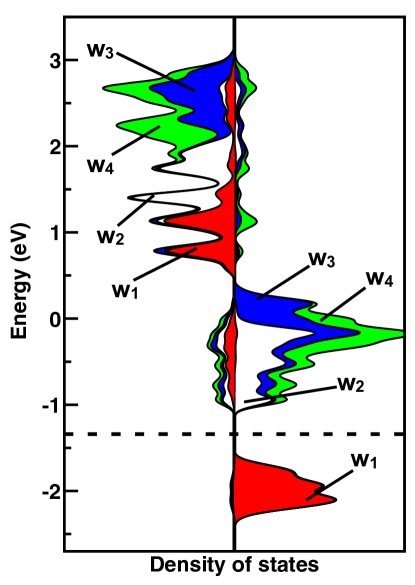
Figure 3: Density of states of the ground state of $\rm{Pr_{\nicefrac{{1}}{{2}}}Ca_{\nicefrac{{1}}{{2}}}MnO_{3}}$ projected on the Wannier-like states $|w_{1}\rangle$ (red), $|w_{2}\rangle$ (white), $|w_{3}\rangle$ (blue) and $|w_{4}\rangle$ (green). The axis of the majority-spin direction points right and that of the minority-spin direction points left. (color online)

In our model calculations, the charge on the central site is 3.75 e and that of the corner site is 3.25 e, which corresponds to a charge disproportion of $q/e=3.5\pm\delta$ with $\delta=0.25$. This value lies within the range of values obtained from various experimental probes as discussed earlierSotoudeh et al. (2017).

The shape of the orbital $|w_{1}\rangle$ is responsible for the orbital order with strong orbital polarization on the central size and negligible orbital polarization on the corner sites. Thus, the electronic structure is consistent with both, the observed Jahn-Teller pattern and the more direct measurements of the charge stateJirak et al. (1985); García et al. (2001); Grenier et al. (2004); Jooss et al. (2007); Mierwaldt et al. (2014)

When the charge order is described in terms of integral charge states, they should be understood as oxidation states, which, per definition, attribute electrons as a whole to the more electronegative partner.McNaught and Wilkinson (1997)

This is, however, a definition rather than a detailed description of an electron distribution. The notion of integral charge states Mn³⁺ and Mn⁴⁺ ions shall be understood in this context. The real charge distributions in manganites are more subtle.

IV Results and discussion

IV.1 Choice of the photon energy

The photo-excitation in manganites occur through both d-to-d and p-to-d transitions in the spectral energy range ${\sim}0.5$-$2.3$ eV Mildner et al. (2015); Sotoudeh et al. (2017); Loshkareva et al. (2004); Hartinger et al. (2006); Quijada et al. (1998). While the d-to-d transitions occur between Mn-3d states, the p-to-d transitions occur between O-2p and Mn-d states Moskvin et al. (2010); Sotoudeh et al. (2017); Ifland et al. (2017). The transitions observed experimentally in the ${\sim}0.5$-$0.75$ eV energy range are mainly dipole-allowed transitions from the occupied to the unoccupied $\rm{e_{g}}$ states. While d-d transition on a single Mn-site are dipole forbidden, there are dipole-allowed transitions, which involve charge-transfer oscillations between different Mn-sites.Sotoudeh et al. (2017) In this work, we focus entirely on transitions within the Mn $\rm{e_{g}}$ shell. The charge-transfer transitions from O-p to Mn-d states dominate only at comparatively higher energies Mildner et al. (2015); Sotoudeh et al. (2017); Loshkareva et al. (2004); Hartinger et al. (2006); Quijada et al. (1998).

A quantity used to describe the excitation is the photon-absorption density $D_{p}$, which is the total number of photons absorbed per Mn-site and pulse. We calculate it as

$$D_{p}{:=}\frac{\Delta E^{tot}_{f-i}}{N_{Mn}\hbar\omega}$$ (23)

from the energy $\Delta{E}^{tot}_{f-i}$ added by the light-pulse to the system with $N_{Mn}$ Mn ions (see also Fig. 31). The division by the photon energy $\hbar\omega$ and $N_{Mn}$ provides the number $D_{p}$ of absorbed photons per Mn-ion and pulse.

Another quantity, often used to characterize experiments, is the pump-fluence $F_{p}$. It is the energy transmitted to the sample per pulse and unit area. The pump fluence determines together with the pulse duration the intensity of the light-field.

The pump fluence $F_{p}$ is

$$F_{p}=\frac{1}{2}|A_{0}|^{2}\omega^{2}c\varepsilon_{0}\int dt\;g(t)^{2}=\frac{1}{2}|A_{0}|^{2}\omega^{2}c\varepsilon_{0}$$ (24)

where $c$ is speed of light and $\varepsilon_{0}$ is vacuum permeability. With $A_{0}$ we denote the amplitude of the vector potential (see Eq. 7). The photon energy is $\hbar\omega$. Due to the normalization of the pulse-shape function $g(t)$, Eq. 8, the relation Eq. 24 is independent of the pulse duration.

The spectral distribution of the photon-absorption density is shown in Fig. 4.

For the simulations discussed below, we have chosen the photon energy equal to the absorption maximum of $\hbar\omega=$1.17 eV. The position of the absorption maximum appears to be rather independent of pulse length and light intensity.

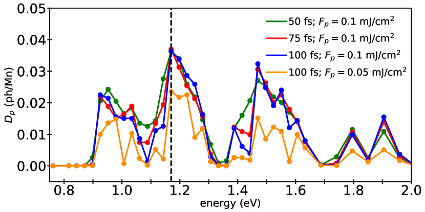
Figure 4: Photon-absorption density $D_{p}$ defined in Eq. 23 as function of the photon-energy $E=\hbar\omega$ for different intensities and pulse lengths. The dashed line indicates the photon-energy $\hbar\omega=1.17$ eV chosen for the simulations described below.

Fig. 5 shows the photon-absorption density $D_{p}$ as a function of the amplitude $A_{0}$ of the light field, as defined in Eq. 7. At the largest fluences, every third electron is excited, which explains the large changes of the magnetic and polaronic microstructure observed in those simulations.

The photon-absorption density in Fig. 5 grows approximately linearly with the amplitude of the light field. This behavior differs from the low fluence regime, where the photon absorption grows quadratically with the amplitude. The approximate linear behavior can be attributed to damping and decoherence. For a two-state system, the optical Bloch equations with damping have a steady state solution with an excited-state population of $P_{e}(A_{0})=A_{0}^{2}/(a+A_{0}^{2})$, where $a$ is constant determined, among others, by detuning and friction parameters.Steck (2019) $P_{e}$ has a point of inflection at a population of 25 %, which explains the approximate linear behavior on the amplitude for the fluences studied here. Additional features seen in Fig. 5 can be attributed in parts to strongly damped Rabi oscillations.

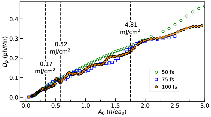
Figure 5: Photon-absorption density $D_{p}$ defined in Eq. 23 as function of the amplitude of the exciting field $A_{0}$ and a photon energy of $\hbar\omega=1.17$ eV. Also given are the pump fluences $F_{p}$ in units of $\rm{mJ/cm^{2}}$ according to Eq. 24 for the boundaries of the four regimes discussed below in section IV.2. (color online)

IV.2 Regimes with distinct relaxation behavior

The relaxation following the optical absorption depends strongly on the pump-fluence $F_{p}$. Based on the diffraction patterns, we identify four regimes with distinct relaxation behavior. The diffraction intensities of the characteristic diffraction spots are shown in Fig. 6. The boundaries of the different regimes depend little on the pulse duration.

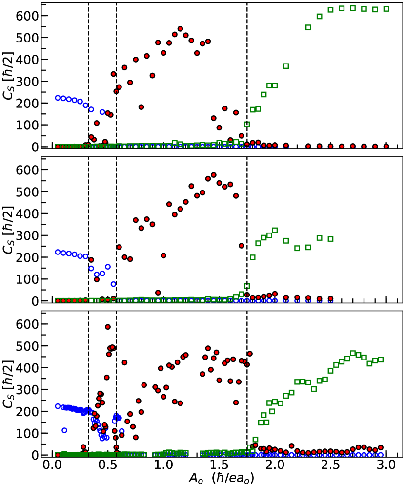
Figure 6: Identification of the distinct regimes on the basis of the intensity of magnetic diffraction spots. The pulse length are 50 fs, 75 fs and 100 fs from top to bottom. Open blue circles show the minimum values of the spin-correlation function $C_{S}(\frac{1}{2},1,1)$ characteristic for the CE-type magnetic structure during the first 2 ps following the excitation. Red-filled circles are the maximum intensities $C_{s}(0,0,1)$ characteristic of the A-type magnetic structure and open green squares are maximum intensities $C_{S}(0,1,1)$ characteristic for the G-type structure. (color online)

The nature of these regimes are discussed in detail below. They can be characterized as follows:

1. In regime I, the spin, charge, and orbital-order is preserved. Coherent phonons with long lifetime are observed.

2. In regime II, the spin dynamics sets in, but the spin pattern relaxes back to the original state on a picosecond time scale. The charge order remains unaffected. Coherent phonons are present as in regime I

3. In regime III and beyond, the charge order is disrupted and the system is driven into a photo-induced ferromagnetic state.

4. In regime IV, the system enters a photo-induced anti-ferromagnetic state.

For the demonstration of the characteristic behavior in the four fluence regimes, we selected the fluence values in Tab. 3.

Table 3: Photon-absorption density $D_{p}$ and fluence $F_{p}$ for the $A_{0}$ values used in the graphs. (color online)

Regime	I	II	III	IV
$A_{0}$($\rm{\hbar/(ea_{0})}$)	0.20	0.45	0.53	2.50
$D_{p}$(ph/Mn)	0.025	0.058	0.094	0.326
$F_{p}$(mJ/cm2)	0.063	0.32	0.44	9.81

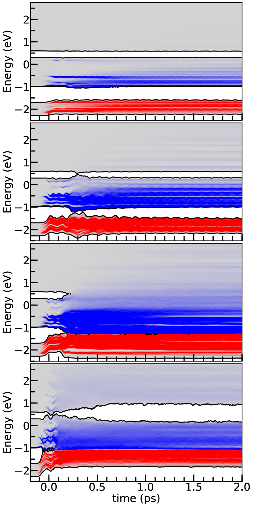
Figure 7: Time evolution of the electron and hole distributions induced by a femtosecond pulse of different intensities. Regime I to IV from top to bottom, i.e. $A_{0}=0.20,0.45,0.53,2.50$ $\rm{\hbar/(ea_{0})}$. The instantaneous one-particle spectrum of Born-Oppenheimer energies is shown in gray. The intensity of blue color indicates conduction electrons and that of red color indicates holes.

The time-dependent distributions of excited electrons and holes are shown in Fig. 7. While the band structure for regimes I and II are qualitatively similar, in regime III the band gap at the Fermi level collapses as a ferromagnetic metallic state is formed. Also the band gap between minority and majority spins collapses. The band gap between majority- and minority-spin orbitals reoccurs in regime IV, where the system evolves into a new antiferromagnetic state. The antiferromagnetism is accompanied by a smaller band width of majority- and minority-spin bands so that the gap between them opens. Like in the ferromagnetic regime III, the system is metallic in regime IV.

IV.3 Regime I

For the weak pump fluences of regime I, the magnetic, charge and orbital orders remain intact. The excitation can be described as formation of electrons and holes in an essentially rigid band structure. The electron-hole pairs are strongly coupled to breathing modes and Jahn-Teller active phonons at the $\Gamma$-point. As a consequence, two coherent phonons with a long lifetime are excited.

The excitation can be rationalized using the Wannier-like states introduced previously. They are shown in Fig. 1 for one segment of the zig-zag chain. Unless mentioned otherwise, the electric field of the light wave points along the b-direction of the Pbnm unit cell, that is along to the zig-zag chains of the ground-state magnetic structure.

IV.3.1 During the light pulse

In the initial phase of the excitation, i.e. during the 100 fs light pulse, charge and orbital order drop to lower values. Furthermore, long-lived oscillations, discussed below, are initiated. On top of these effects, high-frequency oscillations of the electronic system are induced that, however, decay after few tenths of picoseconds. These oscillations are apparent in the charge-order and orbital-order diffraction peaks in Fig. 8 and Fig. 9.

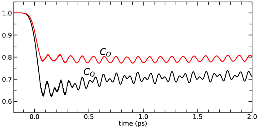
Figure 8: Charge-order correlation $C_{Q}(1,0,0)$ (black) and orbital-order correlation $C_{O}(0,\frac{1}{2},0)$ (red) as function of time for regime I with $A_{0}=0.2$ $\rm{\hbar/(ea_{0})}$. The correlations are scaled each so that their initial value is unity. The correlations can be represented well by a superposition of two harmonic oscillations with frequency $\nu_{1}=10$ THz and $\nu_{2}=16$ THz, which are the frequencies of the two coherent phonons. (color online)

The only dipole-allowed transitions are between the bonding orbital $|w_{1}\rangle$ and the non-bonding orbital $|w_{2}\rangle$ as well as between latter, $|w_{2}\rangle$, and the antibonding orbital $|w_{3}\rangle$ with the same spin direction shown in Fig. 1. There are no dipole-allowed transitions to $|w_{4}\rangle$. Furthermore, there are no dipole-allowed transitions between Wannier-like orbitals from different segments of the zig-zag chains.

There is only one type of dipole-allowed transitions from the filled states. It lifts an electron from the majority-spin bonding orbital $|w_{1}\rangle$ to the non-bonding orbital $|w_{2}\rangle$ of the same segment and with the same spin.

The nature of the high-frequency charge oscillation on a segment of the zig-zag chain is rationalized via the Bloch waves of $|w_{1}\rangle$ and $|w_{2}\rangle$ character shown in Fig. 10, which are connected by the optical excitation. The excitation depends on the polarization of the light. Two representative Bloch waves of the initial state with $|w_{1}\rangle$ character and the corresponding final state with $|w_{2}\rangle$ character are shown schematically in Fig. 10 for each polarization in the ab-plane. The product of initial and final state wave functions is proportional to the first-order change of the charge density, which is in turn responsible for the dipole oscillation that couples to the light field.

For an electric field along the a-axis, i.e. perpendicular to the zig-zag chains, large dipole oscillations between the two corner sites are visible in Fig. 9. The charges of the two corner sites (red/green in Fig. 9) oscillate out-of-phase and with the frequency of the light field. They describe the oscillating charge transfer between the corner sites. This is consistent with the Bloch waves (1) and (2) in Fig. 10 for $\vec{e}_{A}||\vec{a}$. The product of initial, $|w_{1}\rangle$ derived, states and final, $|w_{2}\rangle$ derived, Bloch waves lead to charge contributions with alternating sign on the corner sites of a zig-zag chain. The central site (blue in Fig. 9) has a smaller oscillation with twice the frequency of the light-field. This oscillation is due to the rescaling of the $|w_{1}\rangle$ contribution required to maintain a normalized overall wave function, while $|w_{2}\rangle$ is mixed in.

When the electric field is polarized along the b-axis, i.e. parallel to the zig-zag chain, we observe in Fig. 9 only oscillations with small amplitude and with the doubled frequency of the light wave. The two corner sites oscillate in-phase with the doubled frequency. The charges on the central sites oscillate out of phase with the corner sites. This is consistent with the Bloch waves (3) and (4) in Fig. 10: The product of $|w_{1}\rangle$- and $|w_{2}\rangle$-derived waves has contributions only on the corner sites. However, there, the product of two orthogonal orbitals is formed, which does not contribute to the net charge. The net charge dipole coupling to the light field is not apparent in the bulk. It would show up at the surface of the material. Thus, only the second-order charge oscillations describing the charge transfer from the central site to the corner sites is visible in the bulk. The charge oscillations between the corner sites are initially absent and only kick in at later times.

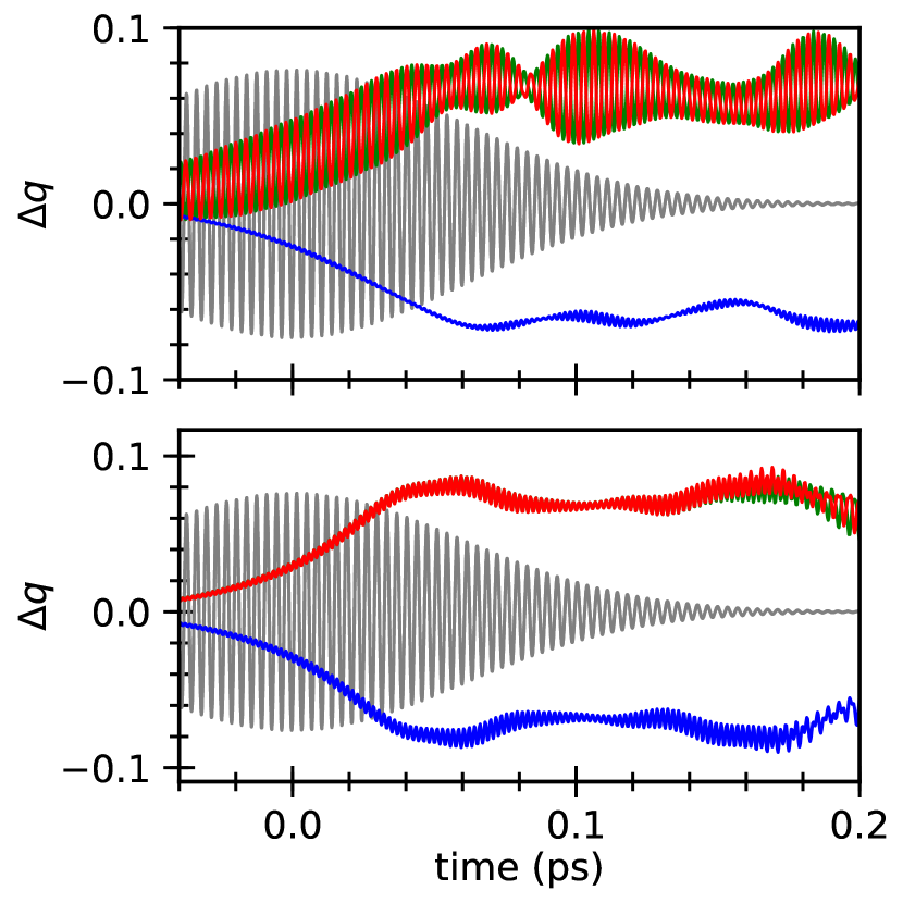
Figure 9: Short-term dynamics for polarization along the a-axis (top) and along the b-axis (bottom) in regime I with $A_{0}=0.20$ $\hbar/(ea_{0})$. Shown are the deviations $\Delta q$ of the charges from a trimer of the CE-type ground state as function of time: central site (blue) and corner sites (red/green). The instantaneous amplitude (arbitrary scale) of the light pulse is shown in grey. (color online)

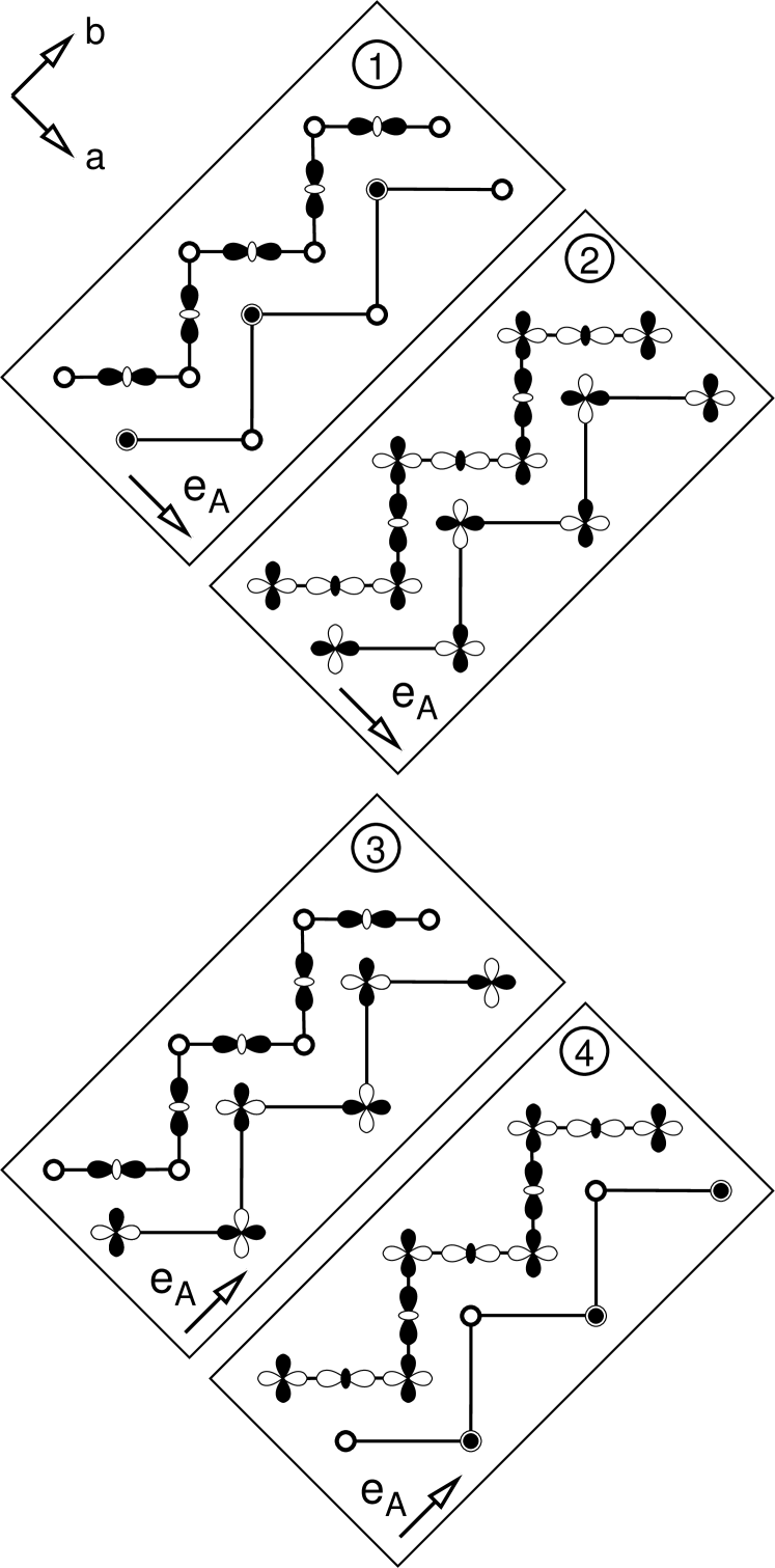
Figure 10: Schematic drawing of Bloch waves involved in the photoexcitation with the electric field $(\vec{E}||\vec{e}_{A})$ polarized perpendicular $(\vec{E}||\vec{a})$ (1) and (2) or along $(\vec{E}||\vec{b})$ (3) and (4) to the zig-zag chains of the CE-type spin order. Each box shows the initial state with $|w_{1}\rangle$-character in the upper left and the final state with $|w_{2}\rangle$-character in the lower right. For each polarization two pairs of initial and final states, one without and one with sign change from one segment to the other, are shown. The induced charge density is related in first order to the product of initial and final state.

IV.3.2 Orbital order

Let us now turn from the high-frequency electronic excitations during the light pulse, to the changes that persist beyond the light pulse.

Figure 11: Total occupancies $F^{tot}_{j}(t)$ (full lines) of Wannier-like orbitals $|w_{j}\rangle$ and their spin polarization $F^{spin}_{j}(t)$ (dashed lines) as function of time for fluence regime I with $A_{0}=0.20$ $\rm{\hbar/(ea_{0})}$. Occupancies of $|w_{1}\rangle$ (red), $|w_{2}\rangle$ (black), $|w_{3}\rangle$ (blue), and $|w_{4}\rangle$ (green). (color online)

For the analysis, we expand the time-dependent one-particle wave functions $|\psi_{n}(t)\rangle$ in Wannier-like orbitals

$$|\psi_{n}(t)\rangle = \sum_{j,\sigma,m}|w_{j,\sigma,m}\rangle\langle w_{j,\sigma,m}|\psi_{n}(t)\rangle$$ (25)

The Wannier-like orbitals $|w_{j,\sigma,m}\rangle$ have spin $\sigma$ ($\sigma\in\{\uparrow,\downarrow\}$) and belong to the trimer $m$ of the unit cell. Index $j$ ($j\in 1,2,3,4$) selects one of the four Wannier-states from a given trimer according to Fig. 1.

The instantaneous occupancy $F_{j}^{tot}(t)$ of the $j$-th Wannier-like state $|w_{j}\rangle$ is

$$F^{tot}_{j} = \frac{2}{N_{Mn}}\sum_{m}\sum_{\sigma}Q_{j,m,\sigma,\sigma}$$ (26)

and its spin polarization is

$$F^{spin}_{j} = \frac{2}{N_{Mn}}$$ (27)

$$\times\sum_{m}\sqrt{(Q_{j,m,\uparrow,\uparrow}-Q_{j,m,\downarrow,\downarrow})^{2}+4Q_{j,m,\uparrow,\downarrow}Q_{j,m,\downarrow,\uparrow}}$$

with the number of Mn-sites $N_{Mn}$ and

$$Q_{j,m,\sigma,\sigma^{\prime}} = \sum_{n}\langle w_{j,\sigma,m}|\psi_{n}\rangle f_{n}\langle\psi_{n}|w_{j,\sigma^{\prime},m}\rangle\;.$$ (28)

As shown in Fig. 11, the dipole-allowed optical transitions from $|w_{1}\rangle$ to $|w_{2}\rangle$ dominate at the low pump fluences of regime I. Thus, the occupancy of $|w_{2}\rangle$ grows at the expense of $|w_{1}\rangle$ during the light pulse, while the occupancies of $|w_{3}\rangle$ and $|w_{4}\rangle$ remain small. After the light-pulse, the occupation of $|w_{2}\rangle$ remain almost constant, which is one sign of the preservation of the ordered state of the material.

Often, e.g. Beaud et al. (2014), the excitation is attributed to an onsite d-to-d transition at the central Mn-site of a trimer segment, which formally is the Mn³⁺-ion. The picture, which emerges from our calculations, is more subtle. Rather than a dipole-forbidden excitation on central Mn-ion from $|w_{1}\rangle$ to $|w_{4}\rangle$, the excitation is a $|w_{1}\rangle$-to-$|w_{2}\rangle$ charge-transfer excitation, which displaces electrons from the central Mn-ions to the corner Mn-ions. This transition does not exist in the limit of complete charge order. The description in terms of Wannier-like orbitals in Fig. 1 explains the strong optical absorption and it has consequences on the coherent modes described below.

IV.3.3 Charge order

The $|w_{1}\rangle$-to-$|w_{2}\rangle$ re-population rearranges electrons from the central to the corner sites, which reduces the charge disproportionation between central and corner sites. The reduced charge disproportionation reflects on the charge-order correlation $C_{Q}(0,1,0)$ shown in Fig. 8. The light pulse induces a sharp drop of the charge-order diffraction intensity $C_{Q}(1,0,0)$ from the initial value. Then, the intensity oscillates around this reduced intensity, with little sign of recovery during our simulation.

In our simulation, the orbital-order peak $C_{O}(0,\frac{1}{2},1)$ has a characteristic frequency of 10 THz, while the charge-order diffraction peak $C_{Q}(1,0,0)$ exhibits one frequency at 10 THz and a second one at 16 THz.

IV.3.4 Coherent vibrations

The removal of electrons from the central site during the $|w_{1}\rangle$-to-$|w_{2}\rangle$ transition reduces its Jahn-Teller distortion. The sudden change excites a Jahn-Teller mode with $\nu=10$ THz, which affects predominantly the central site. The displacements as function of time are shown in Fig. 12.

The charge transfer from central to the corner sites reduces the charge order and thus induces a planar breathing mode on the corner sites with a frequency of $\nu=16$ THz. Note, that an electron addition to a Mn site populates the Mn-O antibonds, which, in turn, expands the nearest neighbor distances. The expansion of the corner sites also affects the Jahn-Teller vibration on the central site.

On the time scale of a few picoseconds, the vibrations do not dissipate significantly. Furthermore, the phonon modes are fully coherent on the picosecond time scale of our calculation.

We attribute the lack of dissipation to the absence of heat conduction. In an experiment, a limited spot is illuminated and the energy can escape from the illuminated region by heat conduction. In our simulation, this process is prohibited, because the infinite material is illuminated homogeneously.

Another reason for an unexpectedly slow dissipation is the specific non-equilibrium state at hand. The coherent phonons are in contact with a phonon bath that is extremely cold. Thus, the collision probability of the coherent phonon with another one is extremely small.

Pump-probe reflectivity measurementsMatsuzaki et al. (2009) of $\rm{Nd_{1/2}Ca_{1/2}MnO_{3}}$, another manganite with the CE-type ground state, provided frequencies with 2.5 THz ($82\rm{cm^{-1}}$, 6.7 THz ($224\rm{cm^{-1}}$), 10.2 THz ($339\rm{cm^{-1}})$ and 14.1 THz ($469~{}\rm{cm^{-1}}$). A coherent vibration with 14 THz has been experimentally observed also for $\rm{La_{1/2}Ca_{1/2}MnO_{3}}$Lim et al. (2005) and $\rm{Pr_{\nicefrac{{1}}{{2}}}Ca_{\nicefrac{{1}}{{2}}}MnO_{3}}$ Beaud et al. (2014); Esposito et al. (2018) for a weak photo-excitation, i.e. below a photo-absorption density of $D_{p}<0.01$, and attributed to Jahn-Teller modes.

The two highest frequencies measured in $\rm{Nd_{1/2}Ca_{1/2}MnO_{3}}$ Matsuzaki et al. (2009) at 10.2 THz and 14.1 THz agree very well with those in our simulations. This suggests a different assignment of the coherent vibrational modes: the mode previously assigned to a octahedral rotation mode at 10 THz, is in our simulation a Jahn-Teller oscillation on the central site of a segment. The mode assigned as Jahn-Teller mode at 16 THz, is in our simulation a symmetric breathing mode at the corner sites. Overlapping with the 10 THz vibration, we also find the antisymmetric expansion of the corner sites along the trimer axis. This latter vibration, however, is not coupled to the optical excitation. It should be noted that displacements of the oxygen ions in our model, denoted as the Jahn-Teller and breathing modes, also have a small implicit component from octahedral tilting.

Vibrations observed in the low-frequency range 2.4-7 THzLim et al. (2005); Matsuzaki et al. (2009); Beaud et al. (2014); Raiser et al. (2017); Esposito et al. (2018), have been attributed to A-type ion motion and rotational modes of MnO₆ octahedra. Our model does not describe these low-frequency modes because it does not contain explicit A-type ions. Pure octahedral rotations are not included, because our model does not describe oxygen vibrations perpendicular to the oxygen bridge.

Our description of the coherent phonons differs from that given earlierMatsuzaki et al. (2009) as being due to an instantaneous melting of the charge and orbital order. The picture emerging from our simulations is that of a mechanistic rather than a thermal process.

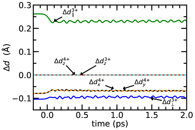
Figure 12: Phonon modes of region I with $A_{0}=0.20$ $\rm{\hbar/(ea_{0})}$. Shown are the expansions $\Delta d$ of the oxygen distances along the octahedral axes. The superscript $3+$ refers to the formal charge state of the central Mn ion in a trimer of the zig-zag chain of the CE-type magnetic structure, while $4+$ refers to the corner site. For the central octahedron, the expansion along the trimer axis is $\Delta d^{3+}_{||}$ and the expansion in the ab-plane perpendicular to the trimer axis is $\Delta d^{3+}_{\perp}$. The planar displacements at the corner atoms along and in the ab-plane perpendicular to the trimer axis $\Delta d^{4+}_{x}$ and $\Delta d^{4+}_{y}$ are identical. The expansions in c-direction, indicated by a subscript $z$ vanish. Visible is the initial reduction of the Jahn-Teller distortion, followed by the coherent breathing mode with 16 THz on the corner sites and a Jahn-Teller mode at the central site with 10 THz. The displacements are averaged over equivalent atoms. (color online)

IV.3.5 Magnetic order

In the fluence regime I, the magnetic order is preserved: The spin angles deviate by about 10 degree from the ideal ground-state arrangement.

IV.4 Regime II: Transient changes of the magnetic order

In the fluence regime II, the Jahn-Teller-active phonons respond similar to regime I. After an initial period of about 200 fs, however, also the spin order is perturbed. The spin system relaxes back into the ground state within few picoseconds, while the reduction of charge and orbital order persists much longer.

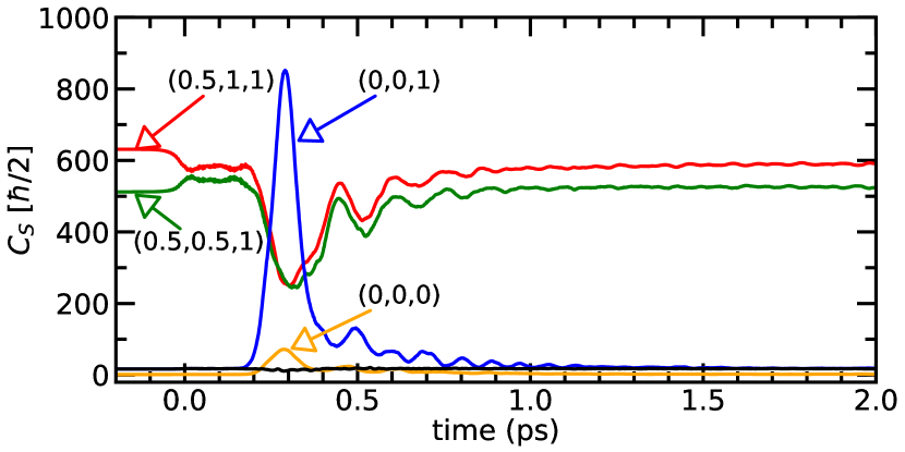
Figure 13: Spin-correlation function of regime II with $A_{0}=0.45$ $\rm{\hbar/(ea_{0})}$. The correlation function $C_{S}(\frac{1}{2},1,1)$ and $C_{S}(\frac{1}{2},\frac{1}{2},1)$ are characteristic for the CE-type ground state. The correlation function $C_{S}(0,0,1)$ is characteristic for A-type magnetic structure. The ferromagnetic (B-type) peak $C_{S}(0,0,0)$ is shown in orange. The CE-type structure recovers after a transient period. (color online)

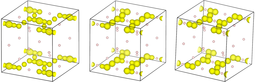
Figure 14: Spin-diffraction patterns in regime II with $A_{0}=0.45$ $\rm{\hbar/(ea_{0})}$. At about 0.29 ps (left), the magnetic structure is a superposition of patterns of the CE-type and the A-type antiferromagnetic structure. At 0.5 ps (middle), a spin-wave emerges, which is similar to obtained in equilibrium with $\delta=15$ % excited electrons (right). (color online)

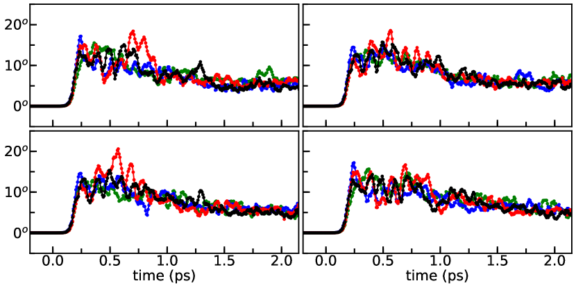
Figure 15: Spin correlations in regime II with $A_{0}=0.45$ $\rm{\hbar/(ea_{0})}$ as function of time. $\Phi_{n,n^{\prime}}$ is the angle between the spins $\langle\vec{S}\rangle_{n}$ of neighboring zig-zag chains $C_{n}$ and $C_{n^{\prime}}$. The mean angle of a chain is $\langle\vec{S}\rangle_{n}=\frac{1}{N}\sum_{j\in C_{n}}\vec{S}_{j}$, where $N$ is the number of Mn-sites in the chain. The top four figures show the angles $\Phi_{n,n^{\prime}}$ for neighboring chains in the same ab plane. The middle four figures show the angles for neighboring chains stacked along the $c$-direction. The bottom four figures show the ferromagnetic spin correlations within a chain $\Delta_{n}=\sqrt{\frac{1}{N}\sum_{j\in C_{n}}\Bigl{[}\angle\Bigl{(}\vec{S}_{j},\langle\vec{S}\rangle_{n}\Bigr{)}\Bigr{]}^{2}}$. (color online)

IV.4.1 Magnetic order

As shown in Fig. 13, the spin correlations of the initial CE-type order drop to lower values at about 0.2 ps, while a prominent but short-lived signal of an A-type magnetic order shows up. This signal lives for about 0.2 ps before it dies out again. The spin-diffraction pattern during this period, which reflects the superposition of CE-type and A-type spin patterns, is shown in the left graph of Fig. 14.

As shown in Fig. 15, the angle of antiferromagnetic neighbors changes by up to 90^∘. Besides some fluctuations, the ferromagnetic order within the zig-zag chain is preserved in the fluence regime II. What is affected most, is the spin correlation between neighboring chains in the ab plane. The onset time decreases with increasing fluence.

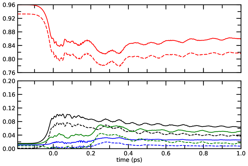
Figure 16: Total occupancies $F^{tot}_{j}(t)$ (full lines) of Wannier-like orbitals $|w_{j}\rangle$ and their spin polarization $F^{spin}_{j}(t)$ (dashed lines) as function of time for fluence regime II with $A_{0}=0.45$ $\rm{\hbar/(ea_{0})}$. Occupancies of $|w_{1}\rangle$ (red), $|w_{2}\rangle$ (black), $|w_{3}\rangle$ (blue), and $|w_{4}\rangle$ (green). (color online)

We attribute the response of the spin system to the optically-induced intersite spin transfer (OISTR)Dewhurst et al. (2018) caused by the coupling of the majority-spin $|w_{2}\rangle$ states with minority-spin states $|w_{1}\rangle$ and $|w_{4}\rangle$ of a neighboring zig-zag chain: the time-dependent populations of the relevant Wannier-like orbitals are shown in Fig. 16. The $|w_{2}\rangle$ state is populated by the photo excitation. It is located at the corner sites and has lobes pointing towards the central atom of a neighboring zig-zag-chain. Thus, there is a spatial overlap of the $|w_{2}\rangle$ orbitals with the minority-spin $|w_{1}\rangle$ and $|w_{4}\rangle$ orbitals of a neighboring chain. The excitation into the $|w_{2}\rangle$ orbital is therefore accompanied by a spin transfer between neighboring zig-zag chains in the ab-plane. The delocalization of electrons among the antiferromagnetically coupled zig-zag chains changes the magnetization of the $\rm{e_{g}}$ electrons, which in turn acts onto the classical spins describing the $\rm{t_{2g}}$ electrons and which causes transient or permanent changes of the magnetization pattern.

In the period from 0.2 to 0.4 ps in Fig. 16, we observe a transfer of weight from $|w_{1}\rangle$ orbitals of one chain to the majority spin $|w_{4}\rangle$ of a neighboring chain. This is a consequence of the transient magnetic transition, which takes place during this period. The hybridization between these orbitals becomes possible because the spin orientation of neighboring chains deviate from $180^{\circ}$.

In order to obtain a better understanding of these spin fluctuations, we investigated the spin structure as function of the ratio of excited electrons. For this purpose, we reduce the occupation for the $\frac{1}{2}N_{Mn}$ occupied states from $1$ to $1-\delta$ and we increase the occupation of the first $\frac{1}{2}N_{Mn}$ unoccupied states from $0$ to $\delta$. Then, we investigate the ground state as function of $\delta$, where all degrees of freedom except strain are relaxed.

The original CE-type spin order is preserved up to $\delta=11$ %. For larger $\delta$, a non-collinear but co-planar spin-wave structure emerges, where every two antiferromagnetic zig-zag chains in the ab-plane pair up and form a finite spin-angle with the spin axis of the next pair. The ferromagnetic spin order within the zig-zag chains and the strict antiferromagnetic coupling in c-direction remain intact. The angle of the spin axes grows with increasing $\delta$ until the angle approaches 90^∘. At this point, $\delta\approx 16$ %, the system collapses into a ferromagnetic metallic state.

Hence, we interprete the spin fluctuation observed in the simulations as the onset of a Néel transition, which, in this case, is driven by photo-excited rather than by thermal $|w_{1}\rangle\rightarrow|w_{2}\rangle$ electron-hole pairs. In this context, the OISTR concept may be generalized to a temperature-induced intersite spin transfer (TISTR).

IV.4.2 Charge order

Charge and orbital order, Fig. 17, as well as coherent phonons, Fig. 18, show the same behavior as in regime I, albeit with larger amplitude. The oscillations of the phonon displacements and the correlation functions for charge and orbital order are long-lived. Unlike regime I, a slow decay of the oscillations is noticeable in regime II.

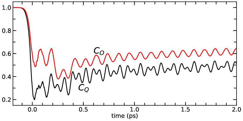
Figure 17: Charge-order correlation $C_{Q}(1,0,0)$ (black) and orbital-order correlation $C_{O}(0,\frac{1}{2},0)$ (red) as function of time for regime II with $A_{0}=0.45$ $\rm{\hbar/(ea_{0})}$. The correlations are scaled each so that their initial value is unity. (color online)

The coherent phonons, charge order, and orbital order are only little affected by the transient change of the magnetic structure. The reason is that the charge order and orbital order remain intact during the transient change of the magnetic correlations.

Coherent phonons, charge order, and orbital order, are strongly coupled via electron-phonon coupling. They are due to the same physical mechanism, namely the $|w_{1}\rangle$ to $|w_{2}\rangle$ excitation. Thus, they are expected to exhibit similar decay properties.

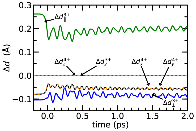
Figure 18: Phonon modes of regime II with $A_{0}=0.45$ $\rm{\hbar/(ea_{0})}$. For a description of the symbols see Fig. 12. (color online)

IV.5 Regime III: Photo-induced ferromagnetism

In regime III, the system undergoes a photo-induced phase transition, which converts the CE-antiferromagnetic order into a ferromagnetic metallic state without charge and orbital order.

IV.5.1 Magnetic order

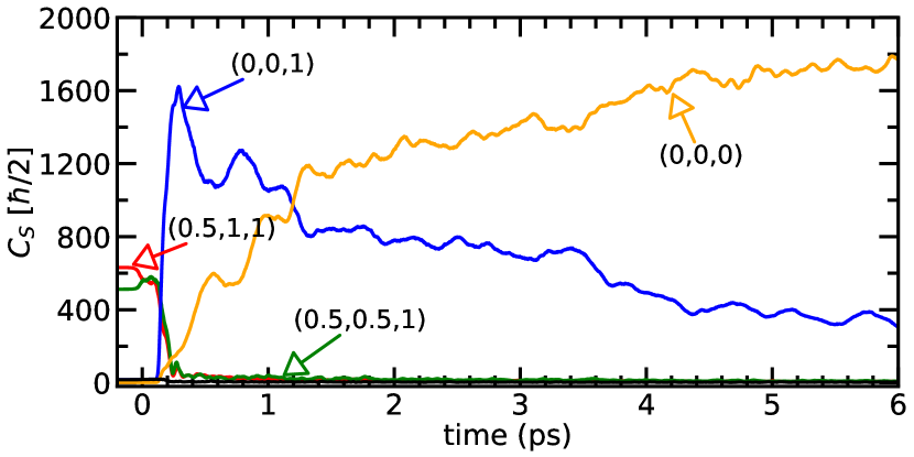
Figure 19: Spin-diffraction intensity of regime III with $A_{0}=0.53$ $\rm{\hbar/(ea_{0})}$. The peaks $C_{S}(0.5,1,1)$ and $C_{S}(0.5,0.5,1)$ shown in red, respectively green, are characteristic for the CE-type ground state. The peak $C_{S}(0,0,1)$ shown in blue is characteristic for A-type magnetic structure. The ferromagnetic (B-type) peak $C_{S}(0,0,0)$ is shown in orange. The original CE-type magnetic pattern is quickly destroyed, while an A-type magnetic pattern emerges. The latter evolves over time into a the ferromagnetic phase. (color online)

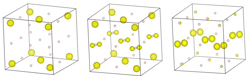
Figure 20: Magnetic diffraction patterns of region III with $A_{0}=0.53$ $\rm{\hbar/(ea_{0})}$ at 0.3 ps, 1.2 ps and 6.1 ps . The a-axis points right, the b-axis towards the back and the c-axis up. The small white spheres indicate points with integer $h,k,l$ in the Pbnm setting. Reciprocal space is shown for $h,k,l\in[-1.25,1.25]$. At 0.3 ps the diffraction pattern is dominated by a A-type pattern. At 1.2 ps the diffraction pattern exhibits spots from both A and B-type, while at 6.1 ps the diffraction pattern is ferromagnetic, i.e. B-type. The double spots are a sign of ferromagnetic magnetic domains, respectively a long-wave length spin wave, rather than a pure ferromagnet. (color online)

Initially, the antiferromagnetic correlation between the zig-zag chains is perturbed rather similar to regime II, leading to an A-type magnetization as seen in Fig. 19. Unlike regime II, however, the A-type diffraction pattern persists for several picoseconds. During this time, the diffraction pattern of the ferromagnet builds up until it replaces the A-type diffraction pattern altogether.

The ferromagnetic state obtained is not fully established in the simulation: The non-relativistic Schrödinger equation employed in the simulations conserves the total spin. As a result, the system evolves into a state that is better characterized as a spin wave or a lattice of ferromagnetic domains.

Nevertheless, the diffraction pattern obtained is very similar to the ferromagnetic structure. For each diffraction spot of the ferromagnetic structure, we do not obtain a single spot, but a set of two “twin-peaks”. The two peaks are located at the supercell reciprocal-space vectors adjacent to those of the ideal ferromagnet as seen in Fig. 20. The displacement of the twin peaks from the diffraction spot of a true ferromagnet is governed by the size of our supercell, which limits the wave length of the spin wave, respectively the domain size.

The ferromagnetic spin correlation function in Fig. 19 exhibits a finite signal by considering the contribution from the immediate neighborhood of the specified reciprocal lattice vector. The signal at the center of the spot is zero.

We envisage that a larger supercell leads to larger domains and thus to twins-peaks that are even closer together, making them indistinguishable by experiment.

IV.5.2 Charge order

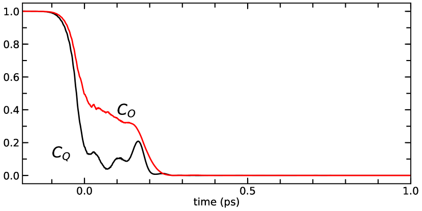
Figure 21: Charge-order correlation $C_{Q}(1,0,0)$ (black) and orbital-order correlation $C_{O}(0,\frac{1}{2},0)$ (red) as function of time for regime III with $A_{0}=0.53$ $\rm{\hbar/(ea_{0})}$. The correlations are scaled each so that their initial value is unity. (color online)

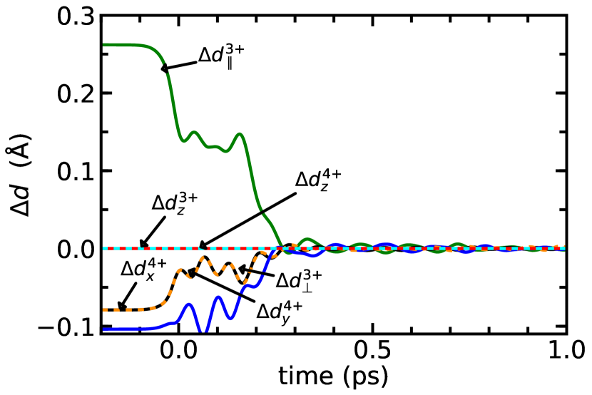
Figure 22: Phonon modes of region III with $A_{0}=0.53$ $\rm{\hbar/(ea_{0})}$. For a description of the symbols see Fig. 12. (color online)

As shown in Fig. 21, the charge-order correlation $C_{Q}$ and the orbital-order correlation $C_{O}$ are completely wiped out after about 0.2 ps. The loss of orbital order makes the system metallic as seen in Fig. 7. The loss in charge and orbital order is also reflected in attenuation of the phonon displacements shown in Fig. 22.

We attribute the ferromagnetic order to a mechanism in the spirit of the double-exchange picture.Zener (1951); Anderson and Hasegawa (1955); Millis et al. (1996) The origin of the band gap in the ground state of $\rm{Pr_{\nicefrac{{1}}{{2}}}Ca_{\nicefrac{{1}}{{2}}}MnO_{3}}$ is the formation of Zener polarons. These Zener polarons are also the origin of charge and orbital order. Due to the re-population of electrons across the band gap, the stabilization due to Zener polarons is lost and another, competing mechanism can take over. A ferromagnetic alignment of the spins lowers the kinetic energy of the electrons, which can now spread over a large area: An electron with a given spin is effectively excluded from orbitals of Mn-ions with opposite spin. A Mn-ion with opposite spin thus leads to an energy cost. Thus, it is favorable, when all spins align ferromagnetically. In other words, a configuration of ferromagnetic spins produces a larger effective band width of the majority-spin configuration. The larger band width stabilizes electrons which populate the lower half of the majority-spin band formed.

IV.5.3 Experiment

A recent ultrafast pump-probe experiment Esposito et al. (2018) carried out on $\rm{Pr_{x}Ca_{1-x}MnO_{3}}$ at 100 K with different pump fluences showed that the characteristic charge- and orbital-order reflection peaks of the CE-type ground state disappear for larger fluences $F_{p}{>}2.5$ $\rm{mJ/cm^{2}}$.

The experimental study with the same material class by Li et al.Li et al. (2013) revealed a photo-induced ferromagnetic state within about 120 fs above the threshold fluence $F_{p}=2.4$ $\rm{mJ/cm^{2}}$. A rise in magnetization has also been measured by Zhou et al.Zhou et al. (2014).

The measured threshold fluence of $F_{p}=2.5$ $\rm{mJ/cm^{2}}$ translates via Eq. 24 into an amplitude $A_{0}=1.26~{}\hbar/(ea_{0})$. In our simulations, the loss of charge and orbital order sets in with $A_{0}=0.58~{}\hbar/(ea_{0})$ ($F_{p}=0.52$ $\rm{mJ/cm^{2}}$) as seen in Fig. 6 from the appearance of the A-type magnetic order, which finally converts into the B-type (ferromagnetic) order. Our simulations and experiments produce the transition in the same fluence range. The remaining difference of a factor five in the threshold fluence may be attributed, for example, to the different photon energies.

It is worth mentioning that the ferromagnetic states observed in our study for region III is expected to persist on longer timescale hinting towards its possible long lifetime. Similar long-lived states are recently observed in $\rm{Pr_{x}Ca_{1-x}MnO_{3}}$ series within the charge-ordered region of the phase diagram Raiser et al. (2017).

IV.6 Regime IV: Non-collinear antiferromagnet

In regime IV with the highest fluence, the system evolves first into a G-type antiferromagnet as shown in Fig. 23, rather than forming an A-type antiferromagnet as in regime III. After about 1.5 ps, the diffraction spots of the G-type structure fall off again in favor of a more complicated structure with non-collinear magnetic order. We note that this regime may be difficult to access experimentally due to the limited stability of the material.

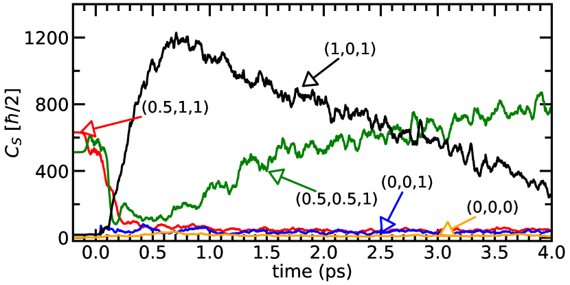
Figure 23: Spin-diffraction intensity of regime IV with $A_{0}=2.50$ $\rm{\hbar/(ea_{0})}$. The peaks $hkl=(0.5,1,1)$ and $(0.5,0.5,1)$ shown in red, respectively green, are characteristic for the CE-type ground state. The ferromagnetic (B-type) peak $C_{S}(0,0,0)$ is shown in orange. The peak with $hkl=(1,0,1)$ is characteristic for G-type magnetic structure. Over time, a new, non-collinear magnetic structure (see Fig. 25) emerges evidenced by the occurrence of the peak $hkl=(0.5,0.5,1)$. (color online)

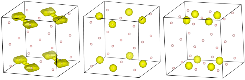
Figure 24: Magnetic diffraction patterns of region IV with $A_{0}=2.50$ $\rm{\hbar/(ea_{0})}$ at 0.3 ps, 0.8 ps and 6.2 ps. At 0.3 ps and 0.8 ps the diffraction pattern is dominated by a G-type pattern. At 6.2 ps a new diffraction pattern occurs, which can be attributed to a non-collinear spin structure described in the text and in Fig. 25. Reciprocal space is shown for $h,k,l\in[-1.25,1.25]$. The a-axis points right, the b-axis towards the back and the c-axis up. The small spheres indicate points with integer $hkl$ in the Pbnm setting. (color online)

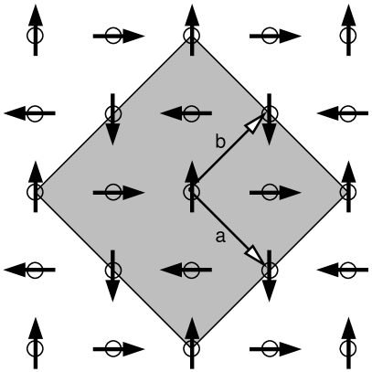
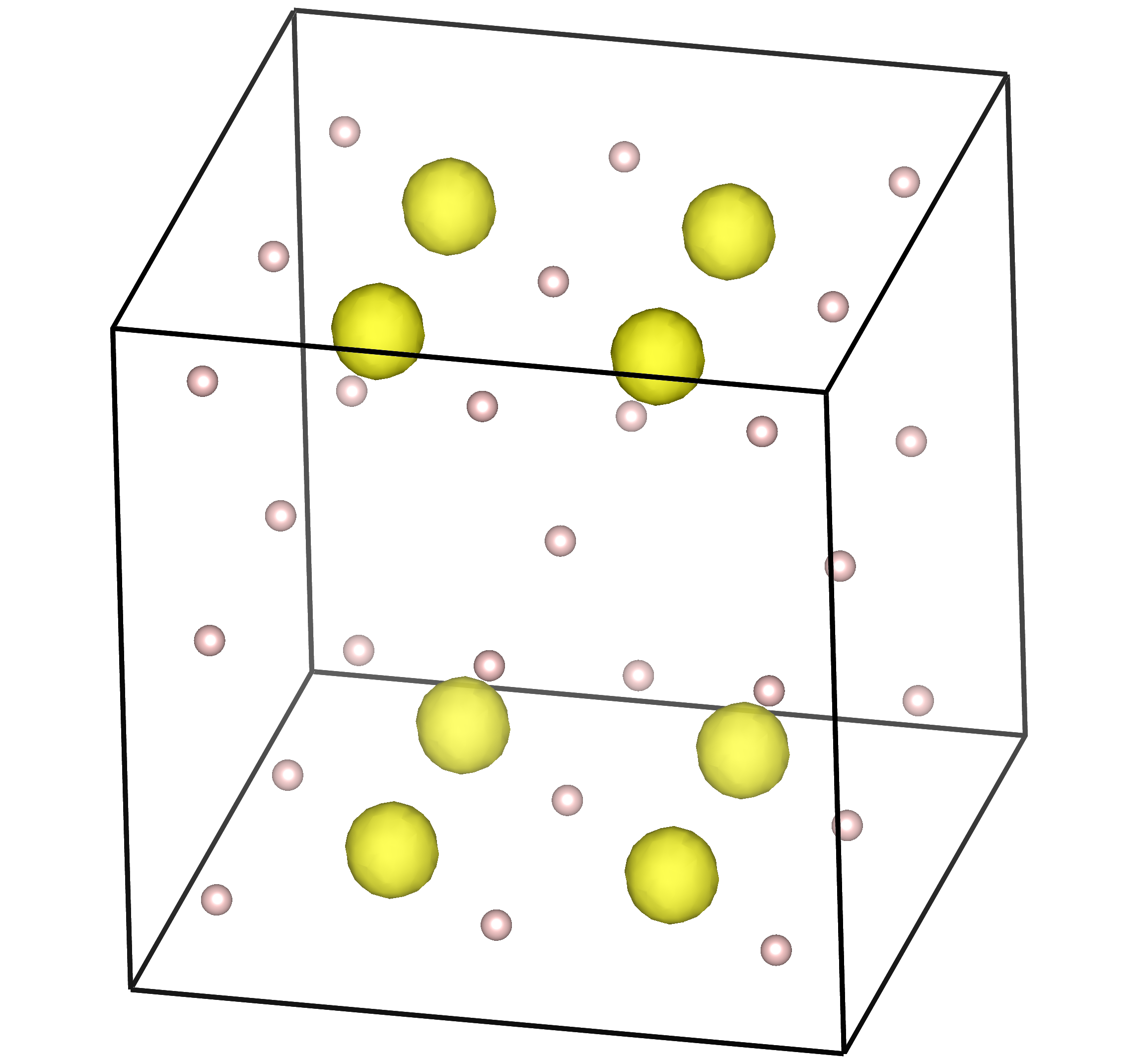
Figure 25: Idealized model for the spin distribution reached in regime IV beyond 2 ps. The non-collinear spin structure in the ab-plane of the Pbnm setting is shown on the left. Shown is the grid of Mn sites with the orientation of the $\rm{t_{2g}}$ spins. Planes are stacked antiferromagnetically in the c-direction. On the right, the corresponding magnetic diffraction pattern is shown. The diffraction pattern is nearly indistinguishable from the one shown in Fig. 24, which is obtained in regime IV at 6.2 ps after the light pulse. The a-axis points right, the b-axis towards the back and the c-axis up. The small spheres indicate points with integer $hkl$ in the Pbnm setting. Reciprocal space is shown for $h,k,l\in[-1.25,1.25]$. (color online)

The diffraction patterns calculated for characteristic times along the trajectory are shown in Fig. 24. The spin structure of the final state, which emerges at approximately 1.5 ps after the light-pulse has been extracted on the basis of the real space spin-correlation function. It is shown in its idealized form in Fig. 25. All spins are perpendicular to its neighbors in the ab-plane and antiferromagnetic in the c-direction. This model produces the spin diffraction pattern of the final spin configuration of regime IV. To our knowledge this configuration has not been investigated before in the context of manganites.

The charge and orbital order is destroyed almost immediately, that is during the light pulse as shown in Fig. 26. This destruction of the orbital order excites phonons, that, however, dissipate on a picosecond time scale as seen in Fig. 27. The amplitude of the phonon vibrations is considerably larger than that in regime III.

We attribute the transition with increasing fluence from a ferromagnet in regime III to the non-collinear antiferromagnetic structure in regime IV to a mechanism analogous to that described earlier.Ono and Ishihara (2017) The double-exchange mechanism favors ferromagnetism through the increase in band width only, when a majority of electrons populate the lower half of the majority-spin $\rm{e_{g}}$ states. Thus, increasing the fluence beyond a certain point switches off the double-exchange mechanism again, so that a antiferromagnetic structure can develop. The reduction of the band width of majority-spin and minority-spin electrons opens a band gap between them, which is seen in Fig. 7. Compared to the minimal modelOno and Ishihara (2017), our system evolves into a more complicated non-collinear antiferromagnetic structure.

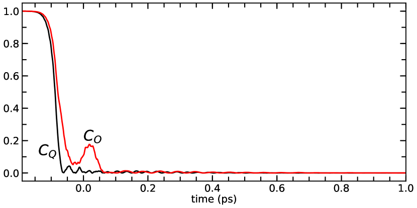
Figure 26: Charge-order correlation $C_{Q}(1,0,0)$ (black) and orbital-order correlation $C_{O}(0,\frac{1}{2},0)$ (red) as function of time for regime IV with $A_{0}=2.5$ $\rm{\hbar/(ea_{0})}$. The correlations are scaled each so that their initial value is unity. (color online)

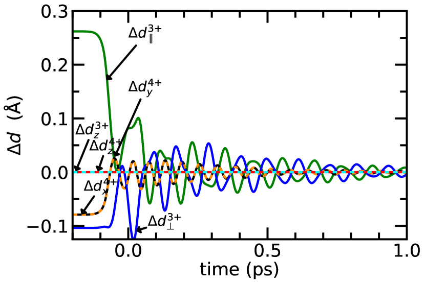
Figure 27: Phonon modes of region IV with $A_{0}=2.50$ $\rm{\hbar/(ea_{0})}$. For a description of the symbols see Fig. 12. (color online)

IV.7 Thermalization

One of the questions of interest is how thermal equilibrium is established from the excited state.

Therefore, we investigated the evolution of the temperatures of the subsystems.

Below, we consider the quasi temperatures described in appendix D.1. As shown in Fig. 28, the light pulse immediately raises the temperature of the electronic system to high temperatures, i.e. several thousands of Kelvin, while the temperatures of the phonon and spin systems remain low in comparison. Thus, a state far from equilibrium is formed. The state is analogous to that of a non-thermal (cold) plasma, where the electrons reach $10^{4}$ K, while the ions remain near room temperature.

While the temperature of the phonon system remains cold, the coherent phonons of regime I and II are strongly coupled to the electronic subsystem and reach comparable temperatures. When we attribute the complete thermal energy of the ions considered to the two phonon modes, the resulting temperature of the two modes is comparable to the electronic temperature.

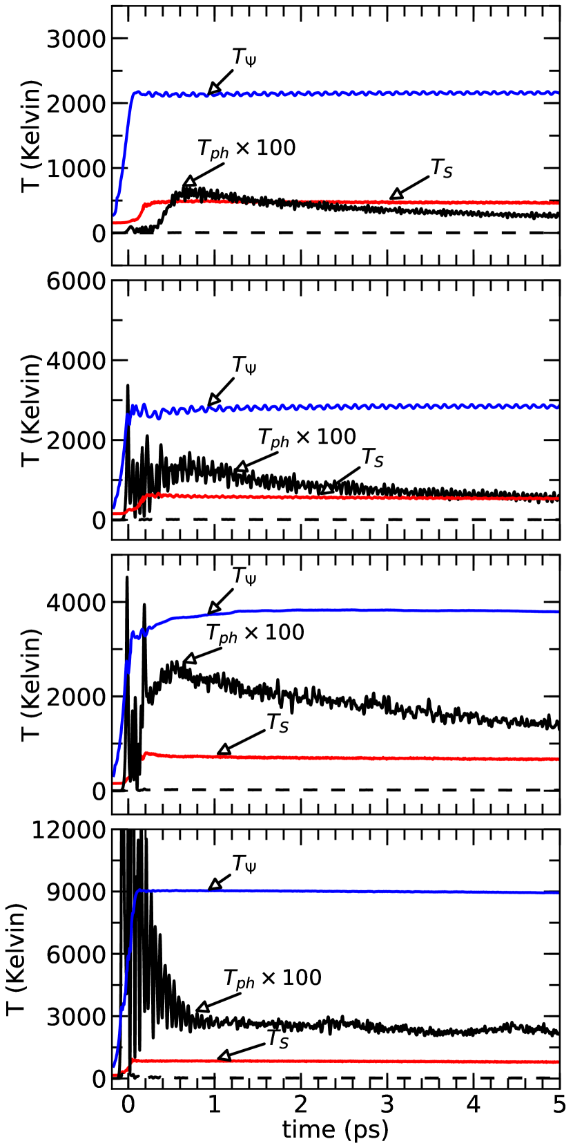
Figure 28: Temperatures of the electron (blue), spin (red)and phonon (black) subsystems as function of time. The phonon temperatures are scaled by 100. From top to bottom are the representative examples from regime I to IV, i.e. $A_{0}=0.20,0.45,0.53$ and $2.50$. (color online)

IV.7.1 Non-equilibrium distribution of the electrons

In particular, the channel of the electrons is of interest because the energy from this channel is most easily put into practical use, such as in a solar cell.

Our simulations may shed light onto the workings of the Boltzmann equation. For this purpose, we inspect the emergence of a distribution, i.e. the occupations, as function of energy and we compare the distribution obtained in our calculation with the Fermi distribution. The approach to a Fermi distribution is one of the common assumptions made for the Boltzmann equation.

In order to explore the approach to the Fermi distribution, we choose a representation of ${\rm atanh}\big{(}1-2\bar{f}_{j}\big{)}$ versus energy $\epsilon^{BO}_{j}$. In this representation, a Fermi distribution maps onto a straight line with slope $1/k_{B}T_{\psi}$ and zero $\mu_{\psi}$.

The Born-Oppenheimer energies $\epsilon^{BO}_{j}$, their occupations $\bar{f}_{j}$ and the Born-Oppenheimer wave functions $|\phi_{j}^{BO}\rangle$ are defined in appendix D.1.2.

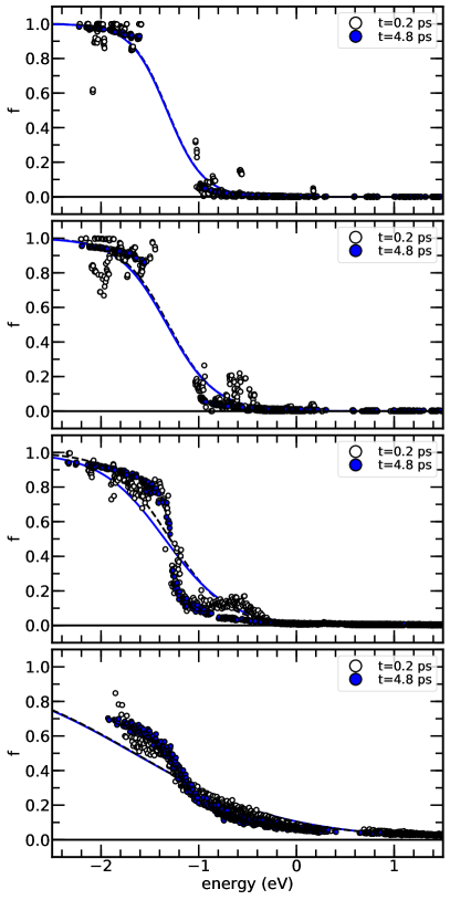
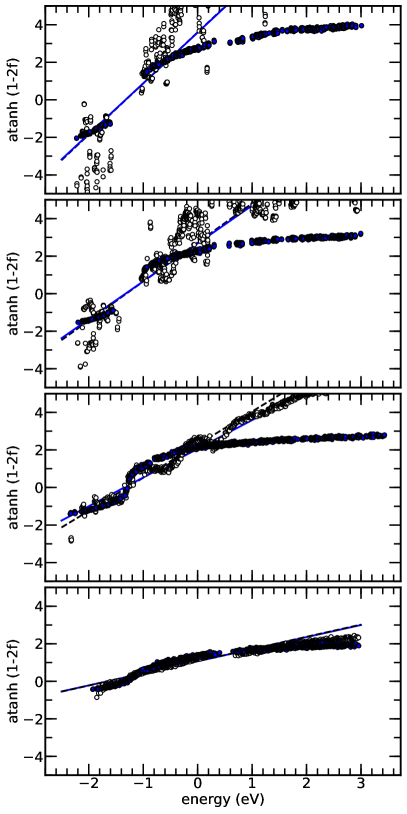
Figure 29: Distributions of electron occupations $\bar{f}$ at different times, namely t=0.2 ps (open circles) and 4.8 ps (blue-filled circles). From top to bottom are the representative examples from regime I to IV, i.e. $A_{0}=0.20,0.45,0.53$ and $2.50$ $\rm{\hbar/(ea_{0})}$. The left figure shows the occupations (circles) versus Born-Oppenheimer energy $\epsilon^{BO}_{j}$. The dashed black line is the Fermi distributions at 0.2 ps obtained from the energy and particle-number sum rules. The full blue line is the Fermi distribution at 4.8 ps. On the right, the occupations $\bar{f}$ are transformed by $\rm{arctanh}(1-2\bar{f})$ which maps a Fermi distribution to a straight line with slope $1/(k_{B}T_{\psi})$ and zero $\mu_{\psi}$. (color online)

The occupations for different time slices and for the four regimes are shown in Fig. 29.

Initially, that is 0.2 ps after the maximum of the light pulse, the occupations do not lie on a continuous function of the one-particle energies but scatter wildly. This is expected because the occupations of the electron states are dominated by the ground-state occupations, the photon energy and the dipole matrix elements.

Already after an initial period of about 0.5 ps after the pulse maximum, the occupations form a continuous function of the energy. This indicates that the thermalization between electrons of the same energy is very efficient.

This result is specific to the choice of one-particle orbitals and energies, namely the Born-Oppenheimer states.

However, on the time scale of our simulation, the system does not approach a Fermi distribution. Rather, occupations of electrons further away from the chemical potential deviate further from integral occupations than a Fermi distribution: The electrons further away from the Fermi level seem to be “hotter” than those close to the Fermi level. Surprisingly, the tails of the distribution become even flatter with time, that is they seem to deviate even further from a Fermi distribution.

We attribute this behavior to the strong coupling between different subsystems: Due to the dynamics of the spin and phonon systems, the electrons experience a time-dependent Hamiltonian, that constantly drives the electrons out of their equilibrium distribution. For the one-particle basis $|\phi^{BO}_{j}(t)\rangle$ used here, the approach to a Fermi distribution is not a requirement.

IV.7.2 Cold-plasma model

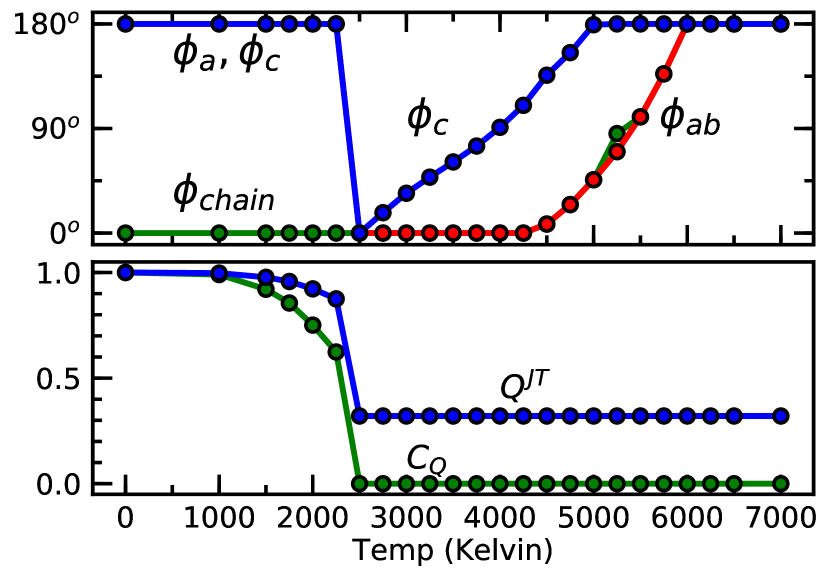
Figure 30: Non-equilibrium phase diagram with hot electrons and cold spins and phonons. Top: spin angles. $\phi_{c}$ is the spin angle between spins in the $c$ direction of the Pbnm setting. $\phi_{ab}$ is the spin angle of neighboring Mn-sites in the ab-plane. Below $T=T_{1}$, the angle $\phi_{ab}$ is replaced by one angle $\phi_{a}$ perpendicular to the zig-zag chains of the CE-magnetic structure and $\phi_{chain}$ is the angle within the zig-zag chains. Bottom figure: Charge-order correlation function $C_{Q}$ and Jahn-Teller distortion $Q^{JT}$ of the central site as function of temperature. Both are divided by their zero-temperature value. (color online)

On the picosecond time scale after an excitation, we find a large disparity between the high temperature of the electrons on the one hand and the low temperatures of spins and phonons on the other hand. This suggests that the optically accessed states are the result of thermodynamic equilibrium of the electron system alone. A quasi-equilibrium state such as this has been assumed earlierZeiger et al. (1992).

In order to test this conjecture, we investigated the phase diagram by increasing the temperature of the electrons, while spins and phonons are kept at zero temperature. That is, spins and phonons are optimized for each electron temperature. The lattice constants are kept equal to the values before excitation, because they are usually too slow on the short time scale under consideration.

As shown in Fig. 30, we find four different temperature ranges, which, however, do not directly correspond to the ranges of different excitation behavior.

• For $T<T_{1}$ with $T_{1}\approx 2500$ K, we obtain the charge-ordered phase with CE-type magnetic order. Charge-order correlations and the corresponding Jahn-Teller distortions on the central site vanish at $T_{1}$ with an approximate square-root behavior $\sim(T_{1}-T)^{\alpha}$ with $0<\alpha<1$.

• $T_{1}<T<T_{2}$ with $T_{2}=4200$ K: At $T=T_{1}$ the charge and orbital order is completely lost, and the system transforms abruptly from the CE-type antiferromagnetic structure into a ferromagnet. The system is a pure ferromagnet only at $T=T_{1}$. For $T>T_{1}$ the spin angle $\phi_{c}$ between adjacent ab-planes increases with an approximate square-root-like behavior towards increasing temperatures, i.e. $\phi_{c}\sim(T-T_{1})^{\beta}$ with $0<\beta<1$. The spin orientation alternates between two values from plane to plane.

• $T_{2}<T<T_{3}$ with $T_{3}=5000$ K: At $T=T_{2}$, the spins in the ab-planes become non-collinear. The angle $\phi_{ab}$ between adjacent spins in the ab-plane increases approximately linearly from $0^{\circ}$ to $180^{\circ}$ as the temperature is raised from $T=T_{2}$ to $T=T_{3}$.

• $T>T_{3}$: At $T=T_{3}$, both spin angles, $\phi_{ab}$ and $\phi_{c}$, are $180^{\circ}$, which corresponds to the G-type magnetic order. This is the favorable high-temperature phase for the temperature range explored.

It is important to note that the phase diagram described here has little to do with the equilibrium phase diagram of the material. The phases described above are extreme non-equilibrium states, because spins and phonons are at $T=0$.

We can identify the excitation regimes I and II with the temperature range $T<T_{1}$. The ferromagnetic state obtained in regime III can be attributed to the range $T_{1}<T<T_{2}$. A non-zero spin angle $\phi_{c}$ between the ferromagnetic planes has not been apparent in our time-dependent simulation. We expect this to be a fluctuating quantity that is averaged out.

In regime IV, we find configurations which are non-collinear in the ab-plane. Interestingly, the non-collinear state with $\phi_{ab}=90^{\circ}$ shown in Fig. 25 is a typical state obtained for a range of fluences, while in Fig. 30 it is just one point in a region with continuously changing angles $\phi_{ab}$. At even higher fluences, also the G-type structure is encountered.

V Summary

The optical excitation of half-doped $\rm{Pr_{0.5}Ca_{0.5}MnO_{3}}$ has been simulated to study the physical interplay between electronic, spin and lattice degrees of freedom in response to a femtosecond light pulse. The simulations use Ehrenfest dynamics, in which electrons and spins follow the time-dependent Schrödinger equation while the nuclei proceed on a classical trajectory.

Femtosecond excitations with various intensities and pulse lengths are studied. The pulse acts on the charge-ordered, low-temperature phase with CE-type antiferromagnetism.

Four different intensity regimes with qualitative different behavior could be identified.

• In regime I, the electron-band structure remains essentially rigid. The electron-hole distribution excitation transfers weight from the central Mn ions of the zig-zag chain to the corner sites. The dipole oscillations shuffle charge between two adjacent corner sites. Two coherent phonons with long life time are excited as result of the electron-phonon coupling.

• In regime II, the spins react and rearrange into short-lived A-type antiferromagnetic structure. The ground-state CE-type antiferromagnetic structure is recovered within a picosecond. The coherent phonons, present also in regime I, survive this transition.

• In regime III, charge and orbital orders are destroyed within few hundred femtoseconds and a ferromagnet is formed. In contrast to regime I and II, the coherent phonons are damped out rapidly. Due to spin conservation, the ferromagnet is not directly accessible. Rather, an A-type antiferromagnet is formed, which evolves over several picoseconds into a ferromagnet having domains compatible with the size of our simulation cell.

• In regime IV, charge and orbital orders are immediately destroyed as in regime III, but now a G-type antiferromagnet is formed rather than an A-type antiferromagnet. Over time, the system evolves into a new non-collinear spin structure with neighboring spins having 90^∘ angles in the ab-plane.

The transient magnetic state observed in regime II may shed light onto the thermal Néel transition of $\rm{Pr_{\nicefrac{{1}}{{2}}}Ca_{\nicefrac{{1}}{{2}}}MnO_{3}}$ at 175 K. In regime II, the system maintains the orbital and charge order, but it modifies the spin correlations of neighboring zig-zag chains of the CE-type spin structure in the ab-plane. Analogously, the Néel transition may be due to a melting of the antiferromagnetic correlations between the zig-zag chains, while maintaining the ferromagnetic order within the chains. When the ferromagnetic order within the chains melts at higher temperature, the integrity of the chains with their orbital and charge order is destroyed as in regime III and IV.

The long lifetime of the magnetic orders in regime III and IV may qualify for the concept of “hidden phases”. Hidden phasesIchikawa et al. (2011) are states with unique order which can not be accessed thermodynamically. It must be noted however, that the time scales covered in our simulations are short compared to those studied experimentally.

In order to make contact with thermodynamics, we estimated the temperatures of the individual subsystems, namely electrons, spins and phonons. The temperature of the electronic subsystem raises quickly to several thousand Kelvin, while phonon and spin degrees of freedom remain relatively “cold”. An exception are the coherent phonon modes, which initially reach the temperature of the electrons before dissipating their energy into other degrees of freedom.

Following this concept of hot electrons and cold phonons and spins, we have been able to identify the phases accessed by optical excitation with those obtained by raising only the electron temperature.

Appendix A Numerical integration of time-dependent Schrödinger equation

To solve the time-dependent Schrödinger equation for wave functions and spinors, we use the second-order differencing scheme proposed by A. Askar and Cakmak.Askar and Cakmak (1978); Kosloff (1988).

Given the wave function $|\psi(0)\rangle$ at time $t=0$ and the time-dependent Hamiltonian $\hat{H}(t)$, the wave function $|\psi(t)\rangle$ can be obtained as $|\psi(t)\rangle=\hat{U}(t,0)|\psi(0)\rangle$ using the propagator

$$\hat{U}(t^{\prime},t)=\mathcal{T}_{D}\exp\left(-\frac{i}{\hbar}\int_{t}^{t^{\prime}}d\tau\;\hat{H}(\tau)\right)\;.$$ (29)

$\mathcal{T}_{D}$ is Dyson’s time-ordering operatorDyson (1949), which rearranges all operators in a product into ascending time order from right to left.

With the time step $\Delta$, subsequent wave functions of a time sequence are related by

$$|\psi_{n}(\Delta)\rangle-|\psi_{n}(-\Delta)\rangle = \Bigl{(}\hat{U}(\Delta,0)-\hat{U}(-\Delta,0)\Bigr{)}|\psi_{n}(0)\rangle$$ (30)

$$=-\frac{2i\Delta}{\hbar}\hat{H}(0)|\psi_{n}(0)\rangle+O(\Delta^{3})\;.$$

The error is reduced by splitting off the dynamical phase using the corresponding energy expectation value $E_{n}(t):=\langle\psi_{n}(t)|\hat{H}(t)|\psi_{n}(t)\rangle$

$${\rm e}^{\frac{i\Delta}{\hbar}E_{n}(0)}|\psi_{n}(\Delta)\rangle-{\rm e}^{-\frac{i\Delta}{\hbar}E_{n}(0)}|\psi_{n}(-\Delta)\rangle$$ (31)

$$= -\frac{2i\Delta}{\hbar}\Big{(}\hat{H}(0)-E_{n}(0)\Big{)}|\psi_{n}(0)\rangle+O(\Delta^{3})\;.$$

This leads to the following iterative scheme

$$|\psi_{n}(t+\Delta)\rangle=|\psi(t-\Delta)\rangle{\rm e}^{-\frac{2i\Delta}{\hbar}E_{n}(t)}$$

$$-\frac{2i\Delta}{\hbar}\Big{(}\hat{H}(t)-E_{n}(t)\Big{)}|\psi(t)\rangle{\rm e}^{-\frac{i\Delta}{\hbar}E_{n}(t)}+O(\Delta^{3})\;.$$ (32)

These equations of motion are time-inversion symmetric per construction.

However, the equations of motion produce besides the correct solution also a spurious partial solution which changes sign in each iteration. This implies that, over time, the wave function will pick up a contribution from the spurious solution. In order to purify the solution, we interrupt the simulation at regular time intervals and perform a correction step. In the correction step, we filter out the spurious partial solution.

$$|\psi^{\prime}(t)\rangle = |\psi(t)\rangle+\frac{1}{4}\Bigl{(}|\psi(t+\Delta)\rangle{\rm e}^{\frac{i}{\hbar}E_{n}(t)\Delta}$$ (33)

$$-2|\psi(t)\rangle+|\psi(t-\Delta)\rangle{\rm e}^{-\frac{i}{\hbar}E_{n}(t)\Delta}\Bigr{)}$$

and perform a Gram-Schmidt orthonormalization on the one-particle wave functions for the two subsequent time steps used in the next iteration.

We use a time step of $\Delta\approx 10^{-3}$ fs. Correction steps are performed every 20 time steps.

The energy conservation is shown in Fig. 31 for different light amplitudes $A_{0}$.

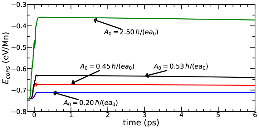
Figure 31: Energy conservation for three intensities of the excitation. The initial rise is due to the excitation. The largest violation of energy conservation is a slow dissipation of the quantum systems. (color online)

Appendix B Spin dynamics

The dynamics of the spins $\vec{S}_{R}$ describing the $\rm{t_{2g}}$ electrons requires special attention. While the spin dynamics is intrinsically of quantum nature, we want to keep all three $\rm{t_{2g}}$ electrons of a given Mn ions strictly collinear. For this purpose, we map the spin vector $\vec{S}_{i}$ onto a normalized, complex-valued, two-component spinor $\left(\begin{array}[]{c}a_{\uparrow,R}\\ a_{\downarrow,R}\\ \end{array}\right)$ such that

$$\vec{S}_{R} = \frac{3\hbar}{2}\left(\begin{array}[]{c}a_{\uparrow,R}^{*}a_{\downarrow,R}+a_{\downarrow,R}^{*}a_{\uparrow,R}\\ -ia_{\uparrow,R}^{*}a_{\downarrow,R}+ia_{\downarrow,R}^{*}a_{\uparrow,R}\\ a_{\uparrow,R}^{*}a_{\uparrow,R}-a^{*}_{\downarrow,R}a_{\downarrow,R}\end{array}\right)\;.$$ (37)

The magnetic moment $\vec{m}_{S}$ of the $\rm{t_{2g}}$ shell is anti-parallel to its spin direction, namely $\vec{m}_{S}=-m_{S}\left(\frac{3\hbar}{2}\right)^{-1}\vec{S}$. The scalar $m_{S}:=|\vec{m}_{S}|$ is defined as the absolute value of the magnetic moment.

The equation of motion is derived from the Lagrangian

$$\mathcal{L} = i\hbar\sum_{\sigma,\alpha,R,n}f_{n}\psi^{*}_{\sigma,\alpha,R,n}\dot{\psi}_{\sigma,\alpha,R,n}+i\hbar\sum_{\sigma,R}a^{*}_{\sigma,R}\dot{a}_{\sigma,R}$$ (38)

$$+\frac{1}{2}\sum_{j=1}^{N_{O}}M_{O}\dot{R}_{j}^{2}-E_{pot}[\psi,S[a],R]\;.$$

The spinors $(a_{\uparrow,R},a_{\downarrow,R})$ evolve under the time-dependent Schrödinger equation

$$i\hbar\partial_{t}\left(\begin{array}[]{c}a_{\uparrow,R}\\ a_{\downarrow,R}\end{array}\right)$$ (41)

$$= m_{S}\left(\begin{array}[]{cc}B_{z,R}&B_{x,R}-iB_{y,R}\\ B_{x,R}+iB_{y,R}&-B_{z,R}\end{array}\right)\left(\begin{array}[]{c}a_{\uparrow,R}\\ a_{\downarrow,R}\end{array}\right)$$ (46)

with

$$m_{S}\vec{B}_{R} = \left(\frac{3\hbar}{2}\right)^{-1}J_{AF}\sum_{R^{\prime}\in{NN_{R}}}\vec{S}_{R^{\prime}}$$ (51)

$$-J_{Hund}\sum\limits_{\alpha}\left(\begin{array}[]{c}\rho_{\downarrow,\alpha,R,\uparrow,\alpha,R}+\rho_{\uparrow,\alpha,R,\downarrow,\alpha,R}\\ -i\rho_{\downarrow,\alpha,R,\uparrow,\alpha,R}+i\rho_{\uparrow,\alpha,R,\downarrow,\alpha,R}\\ \rho_{\uparrow,\alpha,R,\uparrow,\alpha,R}-\rho_{\downarrow,\alpha,R,\downarrow,\alpha,R}\end{array}\right)\;.$$

The summation index $R^{\prime}\in NN_{R}$ runs over nearest-neighbor sites of site $R$. The first term in Eq. 51 describes the antiferromagnetic coupling with neighboring spins. The second term in Eq. 51 describes Hund’s coupling between $\rm{t_{2g}}$ and $\rm{e_{g}}$ electron on the same site. $J_{AF}$ is the antiferromagnetic spin-coupling parameter and $J_{Hund}$ is the Hund’s coupling parameter.

The dynamical equation Eq. LABEL:eq:6 is equivalent to

$$\partial_{t}\vec{S}_{R}=\frac{2m_{S}}{\hbar}\vec{B}_{R}\times\vec{S}_{R}$$ (52)

where $\times$ denotes the vector product.

Appendix C Strain dynamics

In the present study, the scale factors $g_{x}$, $g_{y}$ and $g_{z}$ are dynamical variables, which describe long-wave length acoustic modes that are responsible for the strain effects in manganites Esposito et al. (2018); Lim et al. (2005). We enforce $g_{x}=g_{y}$.

In order to describe the sound wave observed in experiment, we introduce a classical kinetic energy $\frac{1}{2}M_{g}\sum_{m=1}^{3}\dot{g}_{m}^{2}$, which determines the Newton’s equations of motion for the scale factors $g_{m}$.

In thin-film experiments, the wave vector of a sound wave perpendicular to the film is quantized, which results in a standing wave with a characteristic frequency. The sound wave modulates the optical density of the material, which can be detected by the optical absorption measurements.Jang et al. (2010); Zeiger et al. (1992); Thomsen et al. (1984)

We adjusted the fictitious mass $M_{g}$ to simulate this effect. In our model, a sound wave is excited in a material without $\rm{e_{g}}$ electrons with $\vec{q}=0$ and with polarization along the c-direction. $M_{g}$ is chosen so that our model material oscillates with the same frequency as the film in experimentRaiser et al. (2017), namely $\approx 25$ GHz.

Appendix D Peierls substitution

In this section, we give a brief derivation of the Peierls-substitution methodPeierls (1933); Hofstadter (1976).

The electric field $\vec{E}=-\partial_{t}\vec{A}$ of the light pulse is expressed by a vector potential

$$\vec{A}(\vec{r},t)=\frac{\vec{e}_{A}}{2}\Big{(}A_{0}{\rm e}^{i(\vec{k}\vec{r}-\omega t)}+A_{0}^{*}{\rm e}^{-i(\vec{k}\vec{r}-\omega t)}\Big{)}g(t)$$ (53)

$\vec{e}_{A}$ is the polarization direction of the vector potential and $g(t)$ is an envelope function, which is normalized so that

$$\int dt\;|g(t)|^{2}=1\;.$$ (54)

The electrons experience a Hamiltonian of the form

$$\hat{H}[\vec{A}]=\frac{1}{2m_{e}}\Big{(}\hat{\vec{p}}-q\vec{A}(\hat{\vec{r}},t)\Big{)}^{2}+V(\hat{\vec{r}})$$ (55)

where $q$ is the electron charge, $m_{e}$ its mass, and $V$ is the lattice potential.

The Hamilton matrix elements are evaluated in a basisset of local orbitals centered at positions $\vec{R}_{\alpha}$, that have the vector potential explicitly built in. From a regular basisset of local orbitals $|\chi_{\alpha}\rangle$, field-dependent basis functions

$$\langle\vec{r}|\tilde{\chi}_{\alpha}\rangle=\text{exp}\Big{[}\frac{i}{\hbar}q\int_{\vec{R}_{\alpha}}^{\vec{r}}d\vec{r^{\prime}}\vec{A}(\vec{r^{\prime}},t)\Big{]}\langle\vec{r}|\chi_{\alpha}\rangle$$ (56)

are constructedPeierls (1933); Hofstadter (1976). The integral of the vector potential is path dependent: we choose a straight line from the central atom $\vec{R_{\alpha}}$ to the position $\vec{r}$.

Substituting the above ansatz Eq. 56, we obtain

$$\langle\vec{r}|\Big{(}\hat{\vec{p}}-q\vec{A}(\hat{\vec{r}},t)\Big{)}|\tilde{\chi}_{\alpha}\rangle$$

$$=\text{exp}\Big{[}\frac{i}{\hbar}q\int_{\vec{R}_{\alpha}}^{\vec{r}}d\vec{r^{\prime}}\vec{A}(\vec{r^{\prime}},t)\Big{]}\langle\vec{r}|\hat{\vec{p}}|\chi_{\alpha}\rangle$$ (57)

From Eq. 55 and Eq. 57, we obtain

$$\langle\tilde{\chi}_{\alpha}|\hat{H}|\tilde{\chi}_{\beta}\rangle = {\rm e}^{-i\Phi_{\alpha,\beta}(t)}\langle\chi_{\alpha}|{\rm e}^{\frac{i}{\hbar}q\mathcal{F}_{\alpha,\beta}(\hat{\vec{r}},t)}\hat{H}|\chi_{\beta}\rangle$$ (58)

where

$$\Phi_{\alpha,\beta}(t):=\frac{q}{\hbar}\int_{\vec{R}_{\alpha}}^{\vec{R}_{\beta}}d\vec{r^{\prime}}\vec{A}(\vec{r^{\prime}},t)$$ (59)

is the Peierls phase. Furthermore, we define the small quantity $\mathcal{F}_{\alpha,\beta}(\vec{r},t)$, which appears in the above Eq. 58, as

$$\mathcal{F}_{\alpha,\beta}(\vec{r},t) := \int_{\vec{R}_{\alpha}}^{\vec{R}_{\beta}}d\vec{r^{\prime}}\vec{A}(\vec{r^{\prime}},t)+\int_{\vec{R}_{\beta}}^{\vec{r}}d\vec{r^{\prime}}\vec{A}(\vec{r^{\prime}},t)$$ (60)

$$+\int_{\vec{r}}^{\vec{R}_{\alpha}}d\vec{r^{\prime}}\vec{A}(\vec{r^{\prime}},t),$$

$\mathcal{F}_{\alpha,\beta}(\vec{r},t)$ is a magnetic flux through triangle with corners at $\vec{R}_{\alpha},\vec{R}_{\beta}$ and $\vec{r}$.

The time-dependent Schrödinger equation for a wave function $|\psi_{n}(t)\rangle=\sum_{\beta}|\tilde{\chi}_{\beta}(t)\rangle c_{\beta,n}(t)$ obtains the form

$$\sum_{\beta}{\rm e}^{-i\Phi_{\alpha,\beta}(t)}[\tilde{O}_{\alpha,\beta}(t)i\hbar\partial_{t}-\tilde{H}_{\alpha,\beta}(t)]c_{\beta,n}(t)=0$$ (61)

with

$$\tilde{H}_{\alpha,\beta}(t) := \langle\chi_{\alpha}|{\rm e}^{\frac{i}{\hbar}\mathcal{F}_{\alpha,\beta}(\hat{\vec{r}},t)}\Bigl{(}\hat{H}[\vec{0}]+q\int_{\vec{R}_{\beta}}^{\vec{r}}d\vec{r^{\prime}}\dot{\vec{A}}(\vec{r^{\prime}},t)\Bigr{)}|\chi_{\beta}\rangle$$

$$\tilde{O}_{\alpha,\beta}(t) := \langle\chi_{\alpha}|{\rm e}^{\frac{i}{\hbar}\mathcal{F}_{\alpha,\beta}(\hat{\vec{r}},t)}|\chi_{\beta}\rangle$$ (62)

In this form, the Peierls substitution methodPeierls (1933) is formally exact.

In practice, $\mathcal{F}_{\alpha,\beta}(\vec{r},t)$ is neglected. For this to be a good approximation, the basis set needs to be sufficiently localized.

Furthermore, the vector potential is approximated by a constant. This is equivalent to the long-wavelength limit. It also excludes dipole-forbidden, but quadrupole-allowed transitions. The latter are not considered relevant in comparison with the strong charge-transfer transitions in the present work.

With these approximations, by exploiting the orthonormality of our basisset, and after ignoring off-site terms of the dipole matrix elements, we obtain

$$i\hbar\partial_{t}c_{\alpha,n} = \sum_{\beta}{\rm e}^{\frac{-iq}{\hbar}\vec{A}(t)(\vec{R}_{\beta}-\vec{R}_{\alpha})}\langle\chi_{\alpha}|\hat{H}[\vec{0}]|\chi_{\beta}\rangle c_{\beta,n}$$

$$+ \sum_{\beta}\delta_{R_{\alpha},R_{\beta}}\biggl{(}-q\dot{A}(\vec{t})\langle\chi_{\alpha}|\vec{r}-\vec{R}_{\beta}|\chi_{\beta}\rangle\biggr{)}c_{\beta,n}$$

The first term on the right-hand side describes charge-transfer transitions, while the second term describes dipole-allowed onsite transitions. The latter vanish in our model and are included here only for the sake of completeness.

The Peierls phase only affects off-site matrix elements. In our case, these are the hopping matrix elements. Thus, the only change required to incorporate the excitation is to multiply the hopping matrix elements with the time-dependent Peierls phase.

D.1 Temperatures

D.1.1 Phonon temperature

The temperature $T_{ph}$ of the phonon degrees of freedom has been evaluated from the kinetic energy of Jahn-Teller-active and breathing phonon modes of the oxygen ions. We use the relation

$$\sum_{i=1}^{N_{\rm{O}}}\frac{1}{2}M_{O}\dot{\vec{R}}_{i}^{2}=\frac{N_{\rm{O}}}{2}k_{B}T_{ph}$$ (64)

where index $i$ runs over all $N_{\text{O}}$ oxygen ions in the unit cell and $M_{O}$ is the mass of the oxygen ion.

There is only one degree of freedom per oxygen atom in our simulation, because only three phonon modes per formula unit are considered. These are the modes with strong electron-phonon coupling, which receive the energy directly from the excited electrons and holes. Only later, these “hot” modes dissipate their energy into the other phonon modes and the spin system.

D.1.2 Electron temperature

The temperature of the electronic degrees of freedom are obtained from the occupations of the Born-Oppenheimer wave functions. For that purpose, we extract the one-particle wave functions $|\psi_{j}(t)\rangle$ and the instantaneous one-particle Hamiltonian $\hat{h}^{BO}(t)$ acting on the electrons. The Hamiltonian is the Born-Oppenheimer Hamiltonian for the instantaneous spin distribution and atomic positions.

Let $|\phi^{BO}_{j}(t)\rangle$ be the eigenstates and $\epsilon^{BO}_{j}(t)$ the eigenvalues of the one-particle Hamiltonian $\hat{h}^{BO}(t)$. The occupations $\bar{f}_{j}$ of the Born-Oppenheimer states $|\phi^{BO}_{j}(t)\rangle$ are obtained from their projections onto the occupied wave functions $|\psi_{j}(t)\rangle$ as

$$\bar{f}_{j}(t):=\sum_{n=1}^{N_{e}}\left|\langle\psi_{n}(t)|\phi^{BO}_{j}(t)\rangle\right|^{2}\;.$$ (65)

Electron temperature $T_{\psi}$ and electron chemical potential $\mu$ are determined such that energy and particle number coincide with those of a thermal distribution, i.e.

$$\sum_{j}\bar{f}_{j} = \sum_{j}\left({\rm e}^{(\epsilon^{BO}_{j}-\mu)/(k_{B}T_{\psi})}+1\right)^{-1}$$

$$\sum_{j}\bar{f}_{j}\epsilon^{BO}_{j} = \sum_{j}\left({\rm e}^{(\epsilon^{BO}_{j}-\mu)/(k_{B}T_{\psi})}+1\right)^{-1}\epsilon_{j}^{BO}$$ (66)

In order to compare the instantaneous distributions $(\bar{f}_{j},\epsilon_{j})$ to the Fermi distribution $f_{T,\mu}(\epsilon)=1/[1+\exp(\frac{1}{k_{B}T}(\epsilon-\mu))]$, we will plot

$$z(\bar{f})=\mathrm{arctanh}(1-2\bar{f})$$ (67)

because this transforms a Fermi distribution into a linear function of the energy:

$$z\big{(}f_{T,\mu}(\epsilon)\big{)}=\frac{1}{k_{B}T}(\epsilon-\mu)$$ (68)

As a result, we can read the quasi temperature from the slope and the quasi Fermi level from the zero of the interpolated line through the data points $\Big{(}z(\bar{f}_{j}),\epsilon^{BO}_{j}\Big{)}$.

D.1.3 Temperature of the spin subsystem

We extract the temperature of the spin subsystem, i.e. the spins of the $\rm{t_{2g}}$ electrons, analogously to that of the $\rm{e_{g}}$ electrons. For each time step, we extract a Born-Oppenheimer Hamiltonian

$$\mathbf{h}^{BO,S}_{R} := m_{S}\left(\begin{array}[]{cc}B_{z,R}&B_{x,R}-iB_{y,R}\\ B_{x,R}+iB_{y,R}&-B_{z,R}\end{array}\right)$$ (71)

with $\vec{B}_{R}$ defined in Eq. 51 and the absolute value $m_{S}$ of the $\rm{t_{2g}}$ magnetic moment.

The projections of the instantaneous Pauli spinors $\vec{a}_{R}(t)$ onto the eigenvectors $\vec{a}^{BO}_{j,R}(t)$ of $\mathbf{h}^{BO,S}_{R}(t)$ yield occupations

$$\tilde{f}_{j,R}(t)=\biggl{|}\sum_{\sigma\in\{\uparrow,\downarrow\}}a^{*}_{\sigma,R}(t)a^{BO}_{\sigma,j,R}(t)\biggr{|}^{2}$$ (72)

for ground state with $j=0$ and excited state with $j=1$.

The comparison with the internal energy for non-interacting spins in an external magnetic field provides a relation

$$\sum_{R}\Bigl{(}\tilde{f}_{0,R}-\tilde{f}_{1,R}\Bigr{)} = \sum_{R}\tanh\left(\frac{m_{S}|\vec{B}_{R}|}{k_{B}T_{S}}\right)$$ (73)

which is resolved for the instantaneous temperature $T_{S}(t)$ of the spin system.

A more detailed derivation of the expressions summarized here is provided in appendix E.

Appendix E Temperature of the spin subsystem

The temperature of the spin system is extracted analogously to that of the electrons. We consider a system of uncoupled spins in a magnetic-field distribution $\vec{B}_{R}$ defined by the local Born-Oppenheimer Hamiltonian for the spin system according to Eq. 71. The free energy of this system is

$$F_{T}=-k_{B}T\ln\sum_{\vec{\sigma}}{\rm e}^{-\frac{1}{k_{B}T}E_{\vec{\sigma}}}$$ (74)

where the energy of a spin distribution $\vec{\sigma}$ is

$$E_{\vec{\sigma}}=-\sum_{R}m_{S}|\vec{B}_{R}|(-1)^{\sigma_{R}}\;.$$ (75)

$\sigma_{R}\in\{0,1\}$ characterizes the ground and excited state of the local spin $\vec{S}_{R}$ of the $\rm{t_{2g}}$ electrons at site $R$. The absolute value of the magnetic moment related to the spin $\vec{S}_{R}$ of the three $\rm{t_{2g}}$ electrons at a given site is $m_{S}=|\gamma\frac{3\hbar}{2}|$.

This yields for the free energy

$$F_{T}=-k_{B}T\sum_{R}\ln\left[2\cosh\left(\frac{m_{S}|\vec{B}_{R}|}{k_{B}T}\right)\right]$$ (76)

The instantaneous temperature of the spin system is extracted by comparing the energy obtained from the instantaneous spin distribution

$$E(t)=\sum_{R}\vec{a}^{*}_{R}(t)\mathbf{h}^{BO,S}_{R}(t)\vec{a}_{R}(t)$$ (77)

with the energy $\langle E\rangle_{T}=\beta\partial_{\beta}F_{T}$ of the thermal ensemble, where $\beta=1/(k_{B}T)$.

With the eigenstates $\vec{a}^{BO}_{j,R}$ and the eigenvalues $\tilde{\epsilon}_{j,R}$ of the Born-Oppenheimer Hamiltonian $\mathbf{h}^{BO,S}_{R}$, the instantaneous energy Eq. 77 is

$$E(t)=\sum_{R}\tilde{f}_{j,R}(t)\tilde{\epsilon}_{j,R}(t)$$ (78)

with occupations

$$\tilde{f}_{j,R}(t)=\biggl{|}\vec{a}^{*}_{R}(t)\vec{a}^{BO}_{j,R}(t)\biggr{|}^{2}$$ (79)

for the local ground state with $j=0$ and the excited state with $j=1$.

The requirement

$$\sum_{R}\sum_{j=0}^{1}\tilde{f}_{j,R}\tilde{\epsilon}_{j,R} \stackrel{{\scriptstyle!}}{{=}} \beta\partial_{\beta}F_{\beta}=\left\langle E\right\rangle_{T}$$ (80)

provides an expression for the instantaneous temperature $T(t)$

$$\sum_{R}\big{(}\tilde{f}_{0,R}-\tilde{f}_{1,R}\big{)}=\sum_{R}\tanh\left(\frac{m_{S}|\vec{B}_{R}|}{k_{B}T}\right)$$ (81)

Appendix F Frequencies of the coherent phonon modes

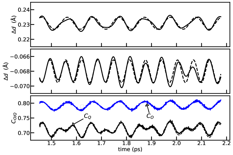
Figure 32: Fit of the phonon modes and diffraction intensities. The top figure shows $\Delta d_{||}^{3+}$ (red) and the fit (dashed). The middle graph shows $\Delta d_{y}^{4+}$ and its fit. The bottom graph are the correlation functions $C_{Q}$ for charge and $C_{O}$ for orbital order and their fits. The derived frequencies are 9.7 THz and 15.7 THz. The trajectory has been performed for a light-amplitude of $A_{0}=0.20$ $\rm{\hbar/(ea_{0})}$. (color online)

The frequencies of the coherent modes, present in regimes I and II, have been extracted by non-linear curve fitting of a superposition of a constant and two cosine functions with amplitude, frequency and phase shift as variable parameters. The quality of the fit is shown in Fig. 32. The fit gives a frequency of 9.7 THz and 15.7 THz.

The vibration of 15.7 THz is dominant in the $\Delta d^{4+}_{y}$ and can be attributed to the planar breathing mode on the corner sites of the CE-type magnetic structure, which couples to the charge transfer from the central to the corner sites.

The lower frequency with $\nu=9.7$ THz is a Jahn-Teller mode on the central site of a trimer.

In order to confirm that the oscillations of the charge- and orbital-order correlation functions are a direct consequence of the coherent phonons, the correlation functions have been fitted with same two frequencies. The perfect agreement shown in Fig. 32 supports our conjecture.

References

- Ren et al. (2008) Y. H. Ren, M. Ebrahim, H. B. Zhao, G. Lüpke, Z. A. Xu, V. Adyam, and Q. Li, Phys. Rev. B 78, 014408 (2008).
- Matsubara et al. (2007) M. Matsubara, Y. Okimoto, T. Ogasawara, Y. Tomioka, H. Okamoto, and Y. Tokura, Phys. Rev. Lett. 99, 207401 (2007).
- Ogasawara et al. (2003) T. Ogasawara, M. Matsubara, Y. Tomioka, M. Kuwata-Gonokami, H. Okamoto, and Y. Tokura, Phys. Rev. B 68, 180407(R) (2003).
- Ichikawa et al. (2011) H. Ichikawa, S. Nozawa, T. Sato, A. Tomita, K. Ichiyanagi, M. Chollet, L. Guerin, N. Dean, A. Cavalleri, S. ichi Adachi, T. hisa Arima, H. Sawa, Y. Ogimoto, M. Nakamura, R. Tamaki, K. Miyano, and S. ya Koshihara, Nature Materials 10, 101 (2011).
- Rini et al. (2007) M. Rini, R. Tobey, N. Dean, J. Itatani, Y. Tomioka, Y. Tokura, R. W. Schoenlein, and A. Cavalleri, Nature 449, 72 (2007).
- Polli et al. (2007) D. Polli, M. Rini, S. Wall, R. W. Schoenlein, Y. Tomioka, Y. Tokura, G. Cerullo, and A. Cavalleri, Nature Materials 6, 643 EP (2007).
- Raiser et al. (2017) D. Raiser, S. Mildner, B. Ifland, M. Sotoudeh, P. Blöchl, S. Techert, and C. Jooss, Advanced Energy Materials 7, 1602174 (2017).
- Prasankumar et al. (2007) R. P. Prasankumar, S. Zvyagin, K. V. Kamenev, G. Balakrishnan, D. M. Paul, A. J. Taylor, and R. D. Averitt, Phys. Rev. B 76, 020402(R) (2007).
- Averitt et al. (2001) R. D. Averitt, A. I. Lobad, C. Kwon, S. A. Trugman, V. K. Thorsmølle, and A. J. Taylor, Phys. Rev. Lett. 87, 017401 (2001).
- Wu et al. (2009) K. H. Wu, T. Y. Hsu, H. C. Shih, Y. J. Chen, C. W. Luo, T. M. Uen, J.-Y. Lin, J. Y. Juang, and T. Kobayashi, J. Appl. Phys. 105, 043901 (2009).
- Bielecki et al. (2010) J. Bielecki, R. Rauer, E. Zanghellini, R. Gunnarsson, K. Dörr, and L. Börjesson, Phys. Rev. B 81, 064434 (2010).
- Lin et al. (2018) H. Lin, H. Liu, L. Lin, S. Dong, H. Chen, Y. Bai, T. Miao, Y. Yu, W. Yu, J. Tang, Y. Zhu, Y. Kou, J. Niu, Z. Cheng, J. Xiao, W. Wang, E. Dagotto, L. Yin, and J. Shen, Phys. Rev. Lett. 120, 267202 (2018).
- Thomsen et al. (1984) C. Thomsen, J. Strait, Z. Vardeny, H. J. Maris, J. Tauc, and J. J. Hauser, Phys. Rev. Lett. 53, 989 (1984).
- Zeiger et al. (1992) H. J. Zeiger, J. Vidal, T. K. Cheng, E. P. Ippen, G. Dresselhaus, and M. S. Dresselhaus, Phys. Rev. B 45, 768 (1992).
- Jang et al. (2010) K.-J. Jang, J. Lim, J. Ahn, J.-H. Kim, K.-J. Yee, and J. S. Ahn, Phys. Rev. B 81, 214416 (2010).
- Sotoudeh et al. (2017) M. Sotoudeh, S. Rajpurohit, P. Blöchl, D. Mierwaldt, J. Norpoth, V. Roddatis, S. Mildner, B. Kressdorf, B. Ifland, and C. Jooss, Phys. Rev. B 95, 235150 (2017).
- Tully (1998) J. C. Tully, Faraday Discuss. 110, 407 (1998).
- Dagotto et al. (2001) E. Dagotto, T. Hota, and A. Moreo, Phys. Rep. 344, 1 (2001).
- Hotta and Dagotto (2002) T. Hotta and E. Dagotto, eprint arXiv:cond-mat/0212466 (2002), cond-mat/0212466 .
- Hotta (2006) T. Hotta, Rep. Prog. Phys. 69, 2061 (2006).
- Müller-Hartmann and Dagotto (1996) E. Müller-Hartmann and E. Dagotto, Phys. Rev. B 54, R6819 (1996).
- McLachlan (1964) A. McLachlan, Mol. Phys. 8, 39 (1964).
- Peierls (1933) R. Peierls, Z. Phys. 80, 763 (1933).
- Hofstadter (1976) D. R. Hofstadter, Phys. Rev. B 14, 2239 (1976).
- Feil (1977) D. Feil, Israel J. Chem. 16, 103 (1977).
- Hotta and Dagotto (2000) T. Hotta and E. Dagotto, Phys. Rev. B 61, R11879 (2000).
- Wollan and Koehler (1955) E. O. Wollan and W. C. Koehler, Phys. Rev. 100, 545 (1955).
- Goodenough (1955) J. B. Goodenough, Phys. Rev. 100, 564 (1955).
- Jirak et al. (1985) Z. Jirak, S. Krupicka, Z. Simsa, M. Dlouha, and S. Vratislav, J. Magn. Magn. Mat. 53, 153 (1985).
- Zimmermann et al. (2001) M. v. Zimmermann, C. S. Nelson, J. P. Hill, D. Gibbs, M. Blume, D. Casa, B. Keimer, Y. Murakami, C.-C. Kao, C. Venkataraman, T. Gog, Y. Tomioka, and Y. Tokura, Phys. Rev. B 64, 195133 (2001).
- García et al. (2001) J. García, M. C. Sańchez, G. Subías, and J. Blasco, J. Phys.: Condens. Matter 13, 3229 (2001).
- Grenier et al. (2004) S. Grenier, J. P. Hill, D. Gibbs, K. J. Thomas, M. v. Zimmermann, C. S. Nelson, V. Kiryukhin, Y. Tokura, Y. Tomioka, D. Casa, T. Gog, and C. Venkataraman, Phys. Rev. B 69, 134419 (2004).
- Jooss et al. (2007) C. Jooss, L. Wu, T. Beetz, R. F. Klie, M. Beleggia, M. A. Schofield, S. Schramm, J. Hoffmann, and Y. Zhu, Proc. Natl. Acad. Sci. USA 104, 13597 (2007).
- Mierwaldt et al. (2014) D. Mierwaldt, S. Mildner, R. Arrigo, A. Knop-Gericke, E. Franke, A. Blumenstein, J. Hoffmann, and C. Jooss, Catalysts 4, 129 (2014).
- McNaught and Wilkinson (1997) A. D. McNaught and A. Wilkinson, eds., IUPAC Compendium of Chemical Terminology, 2nd ed. (Blackwell Scientific Publications, Oxford, 1997).
- Mildner et al. (2015) S. Mildner, J. Hoffmann, P. E. Blöchl, S. Techert, and C. Jooss, Phys. Rev. B 92, 035145 (2015).
- Loshkareva et al. (2004) N. N. Loshkareva, L. V. Nomerovannaya, E. V. Mostovshchikova, A. A. Makhnev, Y. P. Sukhorukov, N. I. Solin, T. I. Arbuzova, S. V. Naumov, N. V. Kostromitina, A. M. Balbashov, and L. N. Rybina, Phys. Rev. B 70, 224406 (2004).
- Hartinger et al. (2006) C. Hartinger, F. Mayr, A. Loidl, and T. Kopp, Phys. Rev. B 73, 024408 (2006).
- Quijada et al. (1998) M. Quijada, J. Černe, J. R. Simpson, H. D. Drew, K. H. Ahn, A. J. Millis, R. Shreekala, R. Ramesh, M. Rajeswari, and T. Venkatesan, Phys. Rev. B 58, 16093 (1998).
- Moskvin et al. (2010) A. S. Moskvin, A. A. Makhnev, L. V. Nomerovannaya, N. N. Loshkareva, and A. M. Balbashov, Phys. Rev. B 82, 035106 (2010).
- Ifland et al. (2017) B. Ifland, J. Hoffmann, B. Kressdorf, V. Roddatis, M. Seibt, and C. Jooss, New Journal of Physics 19, 063046 (2017).
- Steck (2019) D. A. Steck, Quantum and Atomic Optics (available online at http://steck.us/teaching, revision 0.12.6, 23. Apr. 2019, 2019).
- Beaud et al. (2014) P. Beaud, A. Caviezel, S. O. Mariager, L. Rettig, G. Ingold, C. Dornes, S.-W. Huang, J. A. Johnson, M. Radovic, T. Huber, T. Kubacka, A. Ferrer, H. T. Lemke, M. Chollet, D. Zhu, J. M. Glownia, M. Sikorski, A. Robert, H. Wadati, M. Nakamura, M. Kawasaki, Y. Tokura, S. L. Johnson, and U. Staub, Nature Materials 13, 923 (2014).
- Matsuzaki et al. (2009) H. Matsuzaki, H. Uemura, M. Matsubara, T. Kimura, Y. Tokura, and H. Okamoto, Phys. Rev. B 79, 235131 (2009).
- Lim et al. (2005) D. Lim, V. K. Thorsmølle, R. D. Averitt, Q. X. Jia, K. H. Ahn, M. J. Graf, S. A. Trugman, and A. J. Taylor, Phys. Rev. B 71, 134403 (2005).
- Esposito et al. (2018) V. Esposito, L. Rettig, E. Abreu, E. M. Bothschafter, G. Ingold, M. Kawasaki, M. Kubli, G. Lantz, M. Nakamura, J. Rittman, M. Savoini, Y. Tokura, U. Staub, S. L. Johnson, and P. Beaud, Phys. Rev. B 97, 014312 (2018).
- Dewhurst et al. (2018) J. K. Dewhurst, P. Elliott, S. Shallcross, E. K. U. Gross, and S. Sharma, Nano Lett. 18, 1842 (2018).
- Zener (1951) C. Zener, Phys. Rev. 82, 403 (1951).
- Anderson and Hasegawa (1955) P. W. Anderson and H. Hasegawa, Phys. Rev. 100, 675 (1955).
- Millis et al. (1996) A. J. Millis, R. Mueller, and B. I. Shraiman, Phys. Rev. B 54, 5405 (1996).
- Li et al. (2013) T. Li, A. Patz, L. Mouchliadis, J. Yan, T. A. Lograsso, I. E. Perakis, and J. Wang, Nature 496, 69 (2013).
- Zhou et al. (2014) S. Y. Zhou, M. C. Langner, Y. Zhu, Y.-D. Chuang, M. Rini, T. E. Glover, M. P. Hertlein, A. G. C. Gonzalez, N. Tahir, Y. Tomioka, Y. Tokura, Z. Hussain, and R. W. Schoenlein, Scientific Reports 4, 4050 (2014).
- Ono and Ishihara (2017) A. Ono and S. Ishihara, Phys. Rev. Lett. 119, 207202 (2017).
- Askar and Cakmak (1978) A. Askar and A. Cakmak, J. Chem. Phys. 68, 2794 (1978).
- Kosloff (1988) R. Kosloff, J. Phys. Chem. 92, 2087 (1988).
- Dyson (1949) F. J. Dyson, Phys. Rev. 75, 486 (1949).