Multi-group connectivity structures and their implications

Abstract

We investigate the implications of different forms of multi-group connectivity. Four multi-group connectivity modalities are considered: co-memberships, edge bundles, bridges, and liaison hierarchies. We propose generative models to generate these four modalities. Our models are variants of planted partition or stochastic block models conditioned under certain topological constraints. We report findings of a comparative analysis in which we evaluate these structures, controlling for their edge densities and sizes, on mean rates of information propagation, convergence times to consensus, and steady state deviations from the consensus value in the presence of noise as network size increases.

1 Introduction

1.1 Motivation and problem description

As the size of a connected social network increases, multi-group formations that are distinguishable clusters of individuals become a characteristic and important feature of network topology. The connectivity of multi-group networks may be based on co-memberships, edge bundles that connect multiple individuals located in two disjoint groups, bridges that connect two individuals in two disjoint groups, or liaison hierarchies of nodes. Fig. 1 illustrates each form. A large-scale network may include instances of all four connectivity modalities. The work reported in this article is addressed to the implications of these different forms of intergroup connectivity. We set up populations of multiple subgroups and evaluate the implications of different forms of intergroup connectivity structures. We analyze the implications of different forms by adopting standard models of opinion formation and information propagation that allow a comparative analysis on metrics of mean rates of information propagation, convergence times to consensus, and steady state deviations from the consensus value under conditions of noise.

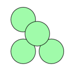
(a) Co-memberships

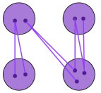
(b) Edge Bundles

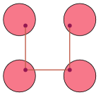
(c) Bridges

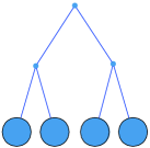
(d) Liaisons

Figure 1: Small-scale illustration of the four forms of multi-group connectivity structures

Typically, a corporation has formal hierarchical structure and additional informal communication structures Likert (1967). The authority of the large-scale organizations is subject to the well-known problem of control loss, i.e., the cumulative decay of influence of superiors over subordinates along the chain-of-command Williamson (1970), Friedkin and Johnsen (2002). Classic and fascinating work on organization cultures Crozier (1964) points to the importance of the topology of informal communication and influence networks in mitigating and exacerbating coordination and control problems. Other work has emphasized particular types of network typologies (linking-pin, bridge, ridge, co-membership, and hierarchical) that may serve as structural bases of mitigating coordination and control loss Likert (1967), Friedkin (1998), Granovetter (1973), Schwartz (1977). In this work we propose generative network models and provide a comparative analysis for these typologies, which we believe are lacking in the literature. Among the multitude of possible coordination and control structures for large groups, we study four prototypical structures and corresponding taxonomy shown in Fig. 1. Bridge connected structure, in which communication between subgroups are based on single contact edges between subgroups; the coordination and control importance of such bridges is the emphasis of the Granovetter (1973) model. According to Granovetter (Granovetter, 1973) only weak ties can be bridges and those weak ties are more likely to be sources of novel information making them surprisingly valuable. Additional references include Tortoriello and Krackhardt (2010), Stam and Elfring (2008), Granovetter (1983), Evans and Davis (2005). Ridge connected or redundant ties structure, in which multiple redundant contact edges connect pairs of groups providing a robust basis of subgroup connectivity; the coordination and control importance of such ridges is the emphasis of Friedkin (1998), Chapter 8. Additional references are Friedkin (1983), White et al. (1976), Boorman and White (1976). Co-membership intersection structures, in which subgroups have common members; the coordination and control importance of such structures is the emphasis of the linking-pin model by Likert (Likert, 1967). This structure represents an organization as a number of overlapping work units in which a member of a unit can belong to other units. Further references include Sawardecker et al. (2009), Cornwell and Harrison (2004), Borgatti and Halgin (2011). Hierarchical connected structure, in which distinct subgroups communicate through liaisons, e.g., a star configuration in which a single individual (who may or may not be in a command role) monitors and facilitates all the work by subgroups and is responsible for all communications among them. Further references are Galbraith (1974), Reynolds and Johnson (1982), Schwartz (1977), Singhal et al. (2014).

We relate the generative models for the first three connectivity structures (co-memberships, edge bundles, and bridges) to stochastic block models (SBMs), which were first introduced in statistical sociology by Holland et al. (PWH-KL-SL:83) and Fienberg & Wasserman (SEF-SSW:81). Also known as planted partition model in theoretical computer science, SBM is a generative graph model that leads to networks with clusters. Conventionally, SBMs are defined for undirected binary graphs and non-overlapping communities. Generalizations of these models to digraphs YJW-GYW:87, overlapping memberships EMA-DMB-SEF-EPX:08, weighted graphs CA-AZJ-AC:14 and arbitrary degree distributions BK-MEJN:11 have also been studied.

In the field of social network science, the four forms of subgroup connectivity illustrated in Fig. 1 are familiar constructs. Comparative research on their implications is limited. Granovetter (Granovetter, 1973) and Watts & Strogatz (Watts and Strogatz, 1998) have focused on the implications of multi-group connectivity based on bridges. Friedkin (Friedkin, 1998) focused on co-membership and edge-bundle connectivity constructs, referring to them as “ridge” structures. Reynolds & Johnson (Reynolds and Johnson, 1982) focused on the importance of liaisons. It may be that ridge structures provide a more robust basis of influence and information flows than thinly dispersed bridges and liaisons. We are unaware of any comparative analysis of all four forms of inter-group connectivity structures that employs a common set of dynamical-system behavioral metrics.

1.2 Statement of contribution

In this article, we develop generative-network models that set up sample networks for each form of multi-group connectivity topology and conduct a comparative analysis of them, which we believe is lacking in the literature. Our models, under some additional constraints, can be regarded as stochastic block models. We compare these network topologies on three metrics: (i) spectral radius, that is a metric of the rate of information propagation in a network propagation models, (ii) convergence time to consensus based on the classic French-DeGroot opinion dynamics, and (iii) steady state deviation from the French-DeGroot consensus value in the presence of noise. We perform a regression analysis to obtain an equitable comparison on the performance of these four connectivity structures and to account for the discrepancies among their structural properties. We learned that the development of generative-network models, suitable for this comparative analysis, is non-trivial. We lay out in detail the assumptions of our models. This is the methodological contribution of the article. The comparative analysis of network metrics, over samples of networks of increasing size in the class of each form of multi-group connectivity, is the article’s theoretical contribution to a better understanding of the implications of these different forms.

For network propagation processes, we refer to the classic references Lajmanovich and Yorke (1976), Hethcote (1978), Allen (1994) and to the recent review Mei et al. (2017). For opinion dynamic processes and the French-DeGroot model, we refer to the classic references French (1956), DeGroot (1974) and the books Friedkin (1998), Jackson (2010), FB:18.

1.3 Preliminaries

Graph theory

Each graph $\mathcal{G(V,E)}$ is identified with the pair $\mathcal{(V,E)}$. The set of graph nodes $\mathcal{V}\neq\emptyset$ represents actors or groups of actors in a social network. $|\mathcal{V}|=n$ is the size of the network. The set of graph links $\mathcal{E}$ represents the social interactions or ties among those actors. We denote the set of neighbors of node $i$ with $\mathcal{N}_{i}$. In a weighted graph, edge weights represent the frequency or the strength of contact between two individuals, whereas in a binary graph all edge weights are equal to one. The density of $\mathcal{G}$ is given by ratio of the number of its observed to possible edges, $\frac{\displaystyle 2|\mathcal{E}|}{\displaystyle n(n-1)}$. Graph $\mathcal{G}$ is called dense if $|\mathcal{E}|=\mathcal{O}(n^{2})$ and sparse if $|\mathcal{E}|\ll n^{2}$. A graph with density of 1 is a clique.

A walk of minimum length between two nodes is the shortest path or geodesic. Average geodesic length is defined by $L=\frac{\displaystyle 1}{\displaystyle n(n-1)}\sum_{i,j\in\mathcal{V},i\neq j}d_{ij}$, where $d_{ij}$ is the length of the geodesic from node $i$ to node $j$. A connected acyclic subgraph of $\mathcal{G}$ spanning all of its nodes is a spanning tree. A uniform spanning tree of size $n$ is a spanning tree chosen uniformly at random in the set of all possible spanning trees of size $n$. Degree or connectivity of node $i$ is defined as the number of edges incident on it. The degree distribution of a graph $P(k)$ is the number of nodes with degree $k$, or the probability that a node chosen uniformly at random has degree $k$. The clustering coefficient of node $i$ is given by the ratio of existing edges between the neighbors of node $i$ over all the possible edges among those neighbors. Letting $c_{i}=\frac{\displaystyle 2e_{jk}:v_{j},v_{k}\in\mathcal{N}_{i},e_{jk}\in\mathcal{E}}{\displaystyle k_{i}(k_{i}-1)},k_{i}=|\mathcal{N}_{i}|$, the average clustering coefficient of graph $\mathcal{G}$ is defined as $C=\frac{1}{n}\sum_{i\in\mathcal{V}}c_{i}$.

An Erdős-Rényi graph Erdős and Rényi (1959) is constructed by connecting nodes randomly. Each edge is included in the graph with a fixed probability $p$ independent from every other edge. We represent such graph as $\mathcal{G}_{ER}(n,p)$ where $p$ is the probability that each edge is included in the graph independent from every other edge. The probability distribution of $\mathcal{G}_{ER}(n,p)$ follows a binomial distribution $P(k)={\binom{n-1}{k}}p^{k}(1-p)^{n-1-k}$, and its average clustering coefficient is given as $C=p$.

Linear algebra

We denote the adjacency matrix of $\mathcal{G}$ with $A\in\mathbb{R}^{n\times n}$ whose $a_{ij}$th entry is equal to the weight of the link between nodes $i$ and $j$ when such an edge exists, and zero otherwise. Matrix $A$ is irreducible if the underlying digraph is strongly connected. If digraph $\mathcal{G}$ is aperiodic and irreducible, then $A$ is primitive. (A digraph is aperiodic if the greatest common divisor of all cycle lengths is $1$.) A cycle is a closed walk, of at least three nodes, in which no edge is repeated.

We adopt the shorthand notations $\mathbbold{1}_{n}=[1,\dots,1]^{\top}$ and $\mathbbold{0}_{n}=[0,\dots,0]^{\top}$. Given $x=[x_{1},\dots,x_{n}]^{\top}\in\mathbb{R}_{n}$, $\operatorname{diag}(x)$ denotes the diagonal matrix whose diagonal entries are $x_{1},\dots,x_{n}$. For an irreducible nonnegative matrix $A$, $\lambda_{\max}$ denotes the dominant eigenvalue of $A$ which is equal to the spectral radius of $A$, $\rho(A)$. The left positive eigenvector of $A$ associated with $\lambda_{\max}$ is called the left dominant eigenvector of $A$.

Empirical networks properties

Our generative-network models attend to three often observed properties of real networks. (i) Small average shortest path: in networks with a large number of vertices, the average shortest path lengths are relatively small due to the existence of bridges or shortcuts. (ii) Heavy tail degree distribution: in contrast to Erdős-Rényi graphs with binomial degree distribution, degree distributions of more realistic networks display a power law shape: $P(k)\sim Ak^{-\alpha}$, where typically $2<\alpha<3$. (iii) High average clustering coefficient: in most real world networks, particularly social networks, nodes tend to create tightly knit groups with relatively high clustering coefficient.

Stochastic block model (SBM)

Let $n,k\in\mathbb{Z}^{+}$ denote the number of vertices and the communities, respectively; $p=(p_{1},\dots,p_{k})$ be a probability vector (the prior) on the $k$ communities, and $W\in\{0,1\}^{k\times k}$ be a symmetric matrix of connectivity probabilities. The pair $(X,\mathcal{G})$ is drawn under the SBM$(n,p,W)$ if $X$ is an $n$-dimensional random vector with i.i.d. components distributed under $p$, and $\mathcal{G(V,E)}$ is a simple graph where vertices $v$ and $u$ are connected with probability $W_{X_{v},X_{u}}$, independently of any other pairs. We define the community sets by $\Omega_{i}=\Omega_{i}(X):=\{v\in\mathcal{V}:X_{v}=i\},i\in\{1,\dots,k\}.$

Note that edges are independently but not identically distributed. Instead, they are conditionally independent, i.e., conditioned on their groups, all edges are independent and for a given pair of groups $(i,j)$, they are i.i.d. Because each vertex in a given group connects to all other vertices in the same way, vertices in the same community are said to be stochastically equivalent. The distribution of $(X,\mathcal{G})$ for $x\in\{1,\dots,k\}^{n}$ is given by:

$$\mathbb{P}\{X=x\}:= \prod\limits_{u=1}^{n}p_{x_{u}}=\prod\limits_{i=1}^{k}p_{i}^{|\Omega_{i}(x)|},$$

$$\mathbb{P}\{\mathcal{E}=y|X=x\}:= \prod\limits_{1\leq u<v\leq n}W_{x_{u},x_{v}}^{y_{uv}}(1-W_{x_{u},x_{v}})^{(1-y_{uv})}.$$

The law of large numbers implies that, almost surely, $\dfrac{1}{n}|\Omega_{i}|\rightarrow p_{i}$.

Symmetric SBM (SSBM) If the probability vector $p$ is uniform and $W$ has all diagonal entries equal to $q_{in}$ and all non-diagonal entries equal to $q_{out}$, then the SBM is said to be symmetric. We say $(X,\mathcal{G})$ is drawn under the SSBM$(n,k,q_{in},q_{out})$, where the community prior is $p=\{1/k\}^{k}$, and $X$ is drawn uniformly at random with the constraints $|\{v\in\mathcal{V}:X_{v}=i\}|=n/k$. The case where $q_{in}>q_{out}$ is called assortative model.

2 Methods

To design our four models we first generate a sequence of group sizes, and refer to the appendix for some of the detailed algorithms involved. Secondly, we produce the community structures according to the sequence of group sizes and add the interconnections among them in the four modalities of multi-group connectivity.

2.1 Generating subgroup sizes

In this section we describe an algorithm to generate relative subgroup sizes, and introduce the resulting properties of these subgroups. We compute a normalized sequence of group sizes with a heavy tail distribution. We refer to Algorithm 1 in the appendix for a formal description based on pseudocode. Each subgroup is modeled as a connected dense Erdős-Rényi graph. For $\epsilon$ substantially smaller than 1 (we shall select it to be $10\%$), a subgroup of size $i$ is the random graph $\mathcal{G}_{ER}(i,1-\epsilon)$.

Each subgroup of size $i$ and edge probability $1-\epsilon$ has the following properties:

1. connectivity threshold of $t(i)=\dfrac{\ln(i)}{i}$, that is, for $1-\epsilon>t(i)$, $\mathcal{G}_{ER}$ is almost surely connected (almost any graph in the ensemble $\mathcal{G}_{ER}$ is connected);

2. $(1-\epsilon)\frac{\displaystyle i(i-1)}{\displaystyle 2}$ edges on average;

3. small average shortest path close to 1 and depending at most logarithmically on $i$;

4. binomial degree distribution: $P(k)=\binom{i-1}{k}(1-\epsilon)^{k}(\epsilon)^{i-1-k}$. Note that as $\epsilon$ decreases, the standard error becomes smaller and the distribution is more densely concentrated around the mean $(i-1)(1-\epsilon)$; and

5. large clustering coefficient close to 1 (conditioned on small $\epsilon$) and equal to $C=1-\epsilon$.

Given a population of $n$ individuals, Algorithm 1 generates a sequence of relative subgroup sizes, such that, when interpreted as a disconnected graph, the collection of these subgroups exhibits a heavy tail degree distribution. An example of subgroup sizes generated by Algorithm 1 is illustrated in Fig. 2.

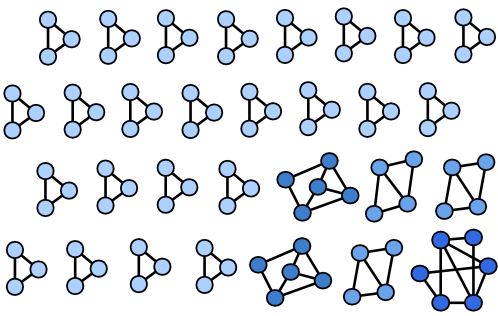
Figure 2: A collection of subgroups on 100 individuals.

As part of Algorithm 1, we design the probability distribution for the subgroup size $i$ to be proportional to $\dfrac{1}{i^{3}}$. The choice of exponent equal to $3$ is based on the following notes: first, in order for $f(i)=\dfrac{k}{i^{\alpha}}$ and its mean to be well-defined, one should have $\alpha\geq 2$; second, if one additionally requires the distribution to have a finite variance, then $\alpha\geq 3$. With exponent 3, the outcome of each realization of the algorithm is a collection of mostly small connected subgroups.

2.2 Models of multi-group connectivity

In this section we describe the algorithms that generate realizations of the four multi-group connectivity modalities.

For three of the four modalities (bridges, edge bundles, and co-members), we connect the subgroups through a minimal set of pairwise coordination problems among them. Specifically, a minimal set of pairwise coordination problems is modeled through the notion of a random spanning tree among the subgroups. To define the generative algorithms for these three structures, we apply the notion of stochastic block models.

2.2.1 Bridge connectivity model

Here we propose an algorithm to generate the bridge connected model. This structure can be modeled as a stochastic block model where the communities are connected through a uniform randomly generated spanning tree, and the interconnections are through precisely one node of each subgroup. We denote the edge set of this random tree with $\mathcal{E}_{T}$. The graph is drawn under the SBM$(n,p,W^{B})$, conditioned under connectivity, where $p$ is calculated by Algorithm 1, and $W^{B}$ is given by:

$$W^{B}_{ij}=\begin{cases}1-\epsilon,&\quad\text{if $i=j$},\\ \dfrac{1}{n^{2}p_{i}p_{j}}=\dfrac{1}{s_{i}s_{j}},&\quad\text{if $i\neq j$ and $ij\in\mathcal{E}_{T}$},\\ 0,&\quad\text{otherwise},\end{cases}$$ (1)

where $s_{i}=|\Omega_{i}|$ denotes the size of group $i$, and $W^{B}$ contains a tree structure. Note that given an SBM, a node in community $i$ has $np_{j}W_{ij}$ neighbors in expectation in community $j$. We illustrate a realization of our algorithm in Fig. 3.

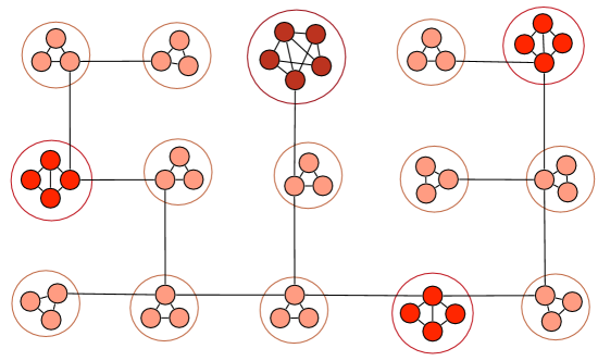
Figure 3: Example of a network of 50 individuals in subgroups connected by bridges.

2.2.2 Edge bundle connectivity model

In this section we propose an algorithm to generate the edge bundle connectivity model. Again we apply a random spanning tree as the building block of the interconnections. Here, instead of adding a single edge as the basis of intergroup connectivity, we add multiple edges whose number grows with the size of the subgroups. We illustrate an algorithm realization in Fig. 4.

We draw the graph under the SBM$(n,p,W^{EB})$, conditioned under redundant connectivity. Communities are connected through a uniform randomly generated spanning tree with edge set $\mathcal{E}_{T}$. The interconnections involve two or more nodes from neighboring subgroups. $p$ is calculated by Algorithm 1, and $W_{EB}$ is given by:

$$W^{EB}_{ij}=\begin{cases}1-\epsilon,&\quad\text{if $i=j$},\\ \dfrac{\alpha_{ij}}{n^{2}p_{i}p_{j}}=\dfrac{\alpha_{ij}}{s_{i}s_{j}},&\quad\text{if $i\neq j$ and $ij\in\mathcal{E}_{T}$},\\ 0,&\quad\text{otherwise},\end{cases}$$ (2)

where $W^{EB}$ contains a tree structure, $\alpha_{ij}=\alpha_{ji}\geq 2$ for all $i,j$, and $\alpha_{ij}$ scales with $s_{i}s_{j}$.

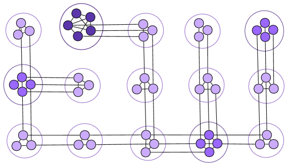
Figure 4: Example of a network of 50 individuals in subgroups connected by bundles of edges.

2.2.3 Co-membership connectivity model

In addition to the existence of a uniform random spanning tree over the subgroup, our co-membership connectivity model generation is conditioned under the following topological constraint: we consider each pair of connected subgroups, say $i$ and $j$, and select a fraction of edges in the complete bipartite graph over $i$ and $j$. For each of these selected edges, we randomly select one of the two individuals, say the individual in $i$, and we turn this individual into a member of the subgroup $j$ by adding edges from this individual to almost all members of $v$.We illustrate an algorithm realization in Fig. 5.

The co-membership model can be generated as a realization of SBM$(n,p,W^{C})$, conditioned under the edge bundles initiated from a single node in one of the corresponding subgroups. Again $\mathcal{E}_{T}$ denotes the edge set of the random tree, $p$ is calculated by Algorithm 1, and $W^{C}$ is given by:

$$W^{C}_{ij}=\begin{cases}1-\epsilon,&\quad\text{if $i=j$},\\ \dfrac{\alpha_{ij}}{n^{2}p_{i}p_{j}}=\dfrac{\alpha_{ij}}{s_{i}s_{j}},&\quad\text{if $i\neq j$ and $ij\in\mathcal{E}_{T}$},\\ 0,&\quad\text{otherwise},\end{cases}$$ (3)

where $W^{C}$ contains a tree structure, $\alpha_{ij}=\alpha_{ji}\geq 3$ for all $i,j$, and $\alpha_{ij}$ scales with either $s_{i}$ or $s_{j}$ ($\alpha_{ij}\approx s_{i}$ or $\alpha_{ij}\approx s_{j}$).

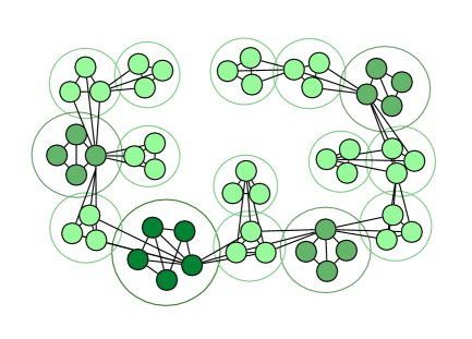
Figure 5: Example of 50 individuals in a co-membership connected network.

2.2.4 Liaison hierarchy connectivity model

Here, applying Algorithm 1 we first generate the subgroups as dense Erdős-Rényi graphs. Then we partition the subgroups into sets of 2 or 3, and (i) assign a liaison to each of sets and (ii) recursively assign a new liaison to groups of 2 or 3 liaisons until we reach the root at the top of the hierarchy. The resulting graph is a hierarchical tree structure with random branching factors of 2 and 3. A detailed description is provided in Algorithm 3 in the appendix, and Fig. 6 illustrates a realization of this model.

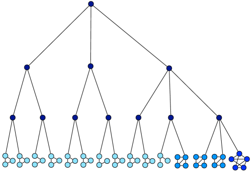
Figure 6: Example of 50 individuals in subgroups joined by a liaison hierarchy generated by Algorithm 3.

3 Results

Realistic networks are usually not exclusively based on a single modality of subgroup connectivity. Our comparative analysis of connectivity modalities is oriented to the question of the implications of a shift away from one modality toward another modality. For example, a modality shift from a liaison hierarchy toward direct bridges among subgroups, or from bridges among subgroups to intergroup edge bundles, or from intergroup edge bundles to co-memberships.

In Fig. 7 we present a comparison of the average shortest paths and average degrees of our generated networks as a function of network size for each of the four multi-group connectivity modalities. Each sample point on the curves is based on 100 realizations on networks with sizes that increase in step sizes of 50 up to 2,000 nodes. In analyses that increase the sample point size to 1,500 over a range of sizes up to 500, there is no marked change in the trajectories. In general, the confidence interval bands are narrow. Here, and elsewhere, red refers to the bridge model, purple to the edge bundle model, green to the co-membership model, and blue to the liaison hierarchy model. Fig. 7a shows that the liaison hierarchy increasingly distinguishes itself from the three modalities as network size increases. Its displayed trajectory is conditional on the liaison structure design. Average shortest paths are insensitive to redundancies. Hence, the lack of distinctions among the other three modalities is not surprising. Fig. 7b shows that the four modalities are systematically ordered with respect to their average degrees: (co-membership) $>$ (edge-bundle) $>$ (bridge) $>$ (liaison) with respect to their average degrees.

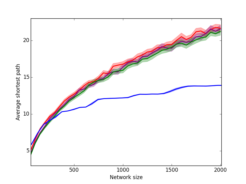
(a) Plot of average shortest path

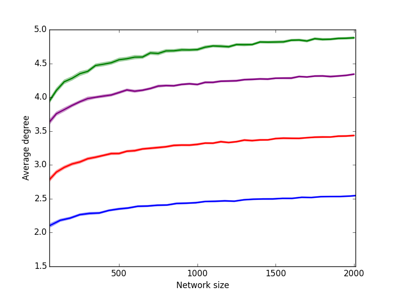
(b) Plot of average degree

Figure 7: In each plot red refers to the bridge model, purple to the edge bundle model, green to the co-membership model, and blue to the liaison hierarchy model

3.0.1 Spectral radius and propagation processes

Propagation phenomena appear in various disciplines, such as spread of infectious diseases, transmission of information, diffusion of innovations, cascading failures in power grids, and spread of wild-fires in forests. Based on the application, the objective can vary from avoiding epidemic outbreaks and eradicating the disease in a population to facilitating the spread of an ideology or product over a network in marketing campaigns. In this subsection we provide a comparison of the system behavior under the simple and well-studied epidemic models proposed in the literature for our four proposed network models.

Let $x(t)=\big{(}x_{1}(t),\dots,x_{n}(t)\big{)}^{\top}$ denote the infection probabilities of each node at time $t$ and $A\in\mathbb{R}^{n\times n}$ denote the adjacency matrix of the contact graph. Let $\beta>0$ be the infection rate, and $\gamma>0$ be the recovery rate to the susceptible state. Then the linearization of the SI (Susceptible-Infected) and SIS (Susceptible-Infected-Susceptible) network propagation models about the no-infection equilibrium point $\mathbbold{0}_{n}$ on a weighted digraph are given by, respectively,

$$\dot{x} =\beta Ax,$$ (4)

$$\dot{x} =(\beta A-\gamma I_{n})x.$$ (5)

The following results are well known (see the classic works Lajmanovich and Yorke (1976), Allen (1994), Wang et al. (2003) and the recent review Mei et al. (2017)). In the SI model the epidemic initially experiences exponential growth with rate $\beta\lambda_{\max}$. In the SIS model near the onset of an epidemic outbreak, the exponential growth rate is $\beta\lambda_{\max}-\gamma$ and the outbreak tends to align with the dominant eigenvector.

In Fig. 8 we plot the spectral radius of the networks as a function of network size 50-2,000 for the four models. In Table 1 we evaluate the differences among these curves controlling a network’s size (N), average degree (Degree), and (0,1) indicator variables for the edge-bundle, co-membership, and liaison modalities with the bridge modality taken as the baseline. Similar findings were obtained with 660K observations on a reduced range of network sizes 24-655. The average degree of a network has a positive effect on the speed of viral propagation. Controlling for network size and average degree, relative to the propagation speeds in the bridge modality, propagation speeds in the edge-bundle and liaison modalities are greater and those of the co-membership modality are less. The elevated curve for co-membership modality in Fig. 8 is based on its systematically higher average degrees.

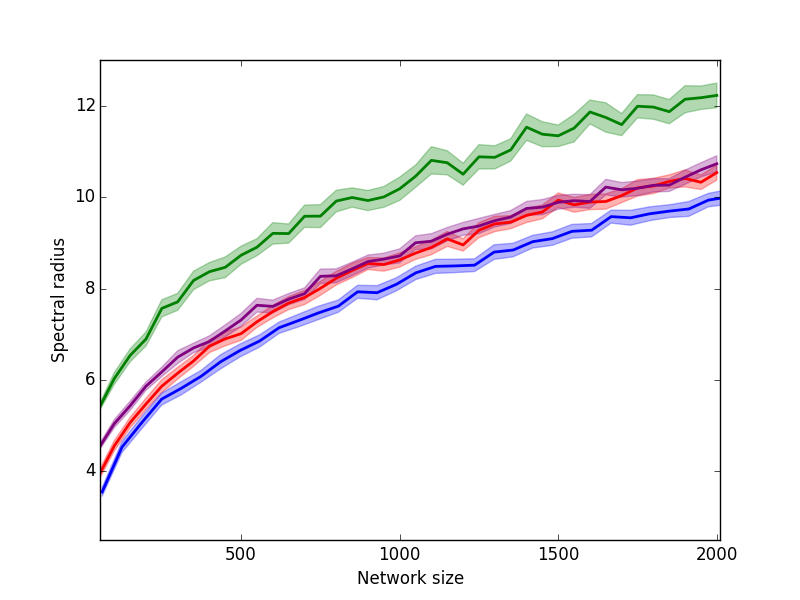
Figure 8: Plot of spectral radius

Table 1: Nonlinear regression results for spectral radius, controlling for network size and average degree, and indicator variables for the connectivity modalities with bridge modality as baseline (15,200 networks, R²= 0.833)

	coeff.	s.e.	p-value
Constant	-2.8103	0.12916	$<$.0001
N	0.0038847	5.2749e-05	$<$.0001
Degree	5.0734	0.088421	$<$.0001
Edge-bundle	0.2012	0.019035	$<$.0001
Co-membership	-1.8589	0.062881	$<$.0001
Liaison	0.24287	0.023229	$<$.0001
N2	-8.3082e-07	2.1709e-08	$<$.0001

3.0.2 Time to convergence in influence processes generating consensus with distributed linear averaging

Consensus algorithms play an important role in many multi-agent systems. They are usually defined as in French-DeGroot discrete-time averaging recursion

$$x(t+1)=Wx(t).$$ (6)

where $W$ is row stochastic and $x(t)\in\mathbb{R}^{n}$ is the vector of individuals’ opinions at time $t$. For primitive stochastic matrices the solution to (6) satisfies

$$\lim_{k\rightarrow\infty}x(k)=\big{(}v^{T}x(0)\big{)}\mathbbold{1}_{n}$$ (7)

where $v$ is the left dominant eigenvector of $W$ satisfying $v_{1}+\dots+v_{n}=1$. Convergence time to consensus may be defined as $\tau_{\textup{asym}}=\frac{\displaystyle 1}{\displaystyle\log(1/r_{\textup{asym}})}$ and it gives the asymptotic number of steps for the error to decrease by the factor $1/e$, where $r_{\textup{asym}}$ denotes the asymptotic convergence factor. It is well known, e.g., see FB:18, Chapter 10, that convergence to consensus is exponentially fast as $\rho_{2}^{t}$, where $\rho_{2}$ is the second largest eigenvalue of $W$ in magnitude. We construct $W$ from $A$ as follows:

$$W=(D+I_{n})^{-1}(A+I_{n}),$$ (8)

where $D=\operatorname{diag}(A\mathbbold{1}_{n})$ denotes the diagonal matrix of all the nodes’ out-degrees, with $d_{ii}=\sum_{j=1}^{n}a_{ij}$ $\forall i$. Equation 8 gives positive weights $w_{ii}$ that are equal to the $w_{ij}$ weights of $i$’s neighbors in $A$.

In Fig. 9, we plot the average convergence-times of the networks as a function of network size 50-2,000 for the four models. In Table 2 we evaluate the differences among these curves controlling a network’s size (N), average degree (Degree), and (0,1) indicator variables for the edge-bundle, co-membership, and liaison modalities with the bridge modality taken as the baseline. Similar findings were obtained with 660K observations on a reduced range of network sizes 24-655. The convergence times of the bridge modality are larger than those of the three other modalities, and the liaison modality has the fastest convergence times. Higher average degrees lower times to convergence. Controlling for network size and average degree, the convergence times of the edge-bundle modality are faster than those of the co-membership modality.

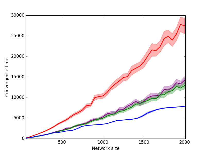
Figure 9: Plot of convergence time for the four network models with equal neighboring weights

Table 2: Nonlinear regression results for convergence time, controlling for network size and average degree, and indicator variables for the connectivity modalities with bridge modality as baseline (15,200 networks, R²= 0.637)

	coeff.	s.e.	p-value
Constant	6991.1	590.12	$<$.0001
N	11.558	0.241	$<$.0001
Degree	-3300.9	403.98	$<$.0001
Edge-bundle	-4652.9	86.969	$<$.0001
Co-membership	-2993.9	287.29	$<$.0001
Liaison	-7790.3	106.13	$<$.0001
N2	-0.0018372	9.9184e-05	$<$.0001

3.0.3 Consensus processes subject to white Gaussian noise

The general form of a French-DeGroot influence process with white Gaussian noise is:

$$x(t+1)=Wx(t)+e(t)$$ (9)

where $e(t)$ is a random vector with zero mean and covariance $\Sigma_{e}$ having independent entries. In the presence of noise, the states of the agents will be brought close to each other, but will not fully align to exact consensus. The resulting noisy consensus is referred to as persistent disagreement. For strongly connected and aperiodic graphs, the consensus dynamics (6) correspond to an irreducible and aperiodic Markov chain. The matrix $W$ then corresponds to the transition probability matrix and its normalized left dominant eigenvector $\pi$ corresponds to the stationary distribution vector of the chain. The results on the steady-state disagreement by Jadbabaie & Olshevsky (Jadbabaie and Olshevsky, 2015) apply to reversible Markov chains which with the choice of weights on our adjacency matrix will be met. For the Markov chain with reversible transition matrix $W$ and with uncorrelated noise, the mean square asymptotic error $\delta_{ss}$ can be measured by:

$$\delta_{ss}=\pi^{T}HD_{\pi}\Sigma_{e}D_{\pi}\mathbbold{1}_{n},$$ (10)

where $D_{\pi}=\operatorname{diag}(\pi)$, and $H$ is the matrix of hitting times for the Markov chain. The algorithm by Kemeny & Snell (Kemeny and Snell, 1976) is applied to compute $H$.

In Fig. 10, we plot the steady-state mean deviation from consensus, given by (10), on the networks as a function of network size 50-2,000 for the four models. In Table 3 we evaluate the differences among these curves controlling a network’s size (N), average degree (Degree), and (0,1) indicator variables for the edge-bundle, co-membership, and liaison modalities with the bridge modality taken as the baseline. Similar findings were obtained with 660K observations on a reduced range of network sizes 24-655. The steady-state mean deviations for the bridge modality are larger than those of the three other modalities. Higher average degrees lower steady-state mean deviations from consensus. Although the modalities have distinguishable effects, again we note that average degree differences are “boiled into” the modality models, so that when average degree is controlled, the relative ordering of modalities is altered. The edge-bundle and liaison modalities have greater noise reduction properties than the co-membership modality.

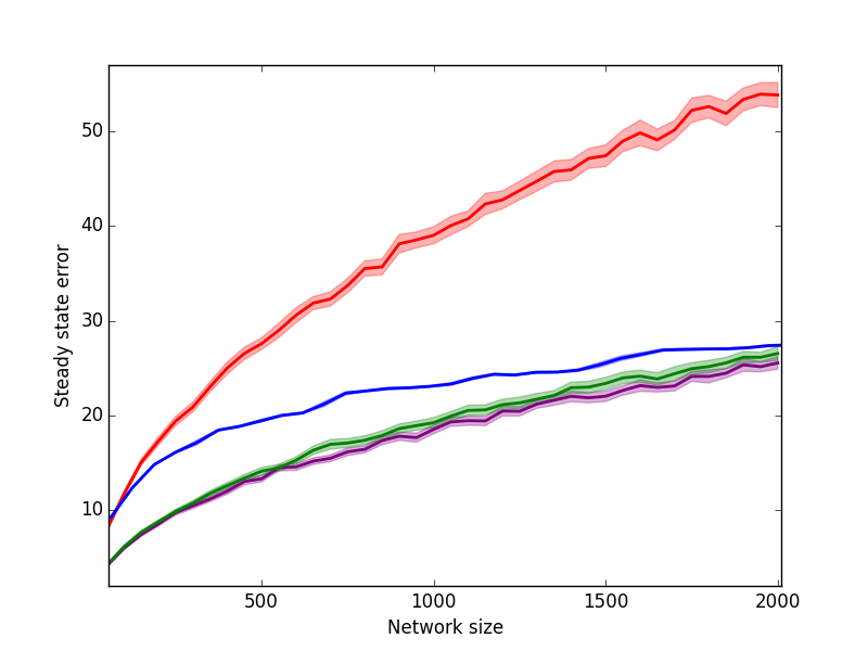
Figure 10: Plot of $\delta_{ss}$ of graph $A$ for the four network models with equal neighboring weights

Table 3: Nonlinear regression results for steady-state mean deviation from consensus, controlling for network size and average degree, and indicator variables for the connectivity modalities with bridge modality as baseline (15200 networks, R²= 0.768)

	coeff.	s.e.	p-value
Constant	30.894	0.84085	$<$.0001
N	0.031003	0.0003434	$<$.0001
Degree	-9.1312	0.57562	$<$.0001
Edge-bundle	-16.807	0.12392	$<$.0001
Co-membership	-10.502	0.40935	$<$.0001
Liaison	-14.052	0.15122	$<$.0001
N2	-9.1291e-06	1.4133e-07	$<$.0001

4 Discussion

In this article, we have proposed simple, synergistic, and stochastic algorithms to generate four modalities of multi-group connectivity and have compared their implications. These algorithms are a variant of what is known as planted partition or stochastic block models, under some further topological constraints including that the intergroup connectivity is shaped by an underlying tree. Models 1-3 are nested in the following sense: for appropriate parameters, 1) graphs generated by the bridge connectivity structure are subgraphs of those generated by the edge bundles, and 2) graphs generated by the edge bundle connectivity structure could be subgraphs of those generated by the co-membership. However, moving from the edge bundles to co-memberships, we introduce an additional constraint, that is, edge bundles of the spanning tree are initiated from the same node in one of neighboring subgroups in the co-membership model. The work touches on two central traditions in network analysis: models of network structure and models of dynamical processes that unfold on networks composed of multiple small groups with dense within-group edges. In a connected network, any two such groups might be intersecting (with one or more individuals who are members of both) or disjoint. Two disjoint subgroups may be linked by a bridge, or by multiple edges, or by individuals who are not members of any dense group. We consider networks that can be strictly characterized in terms of one of these types of inter-group connectivity. The touchstone for our analysis is the work that has been conducted on multiple-group connectivity based on bridges. Here we elaborate the analysis with a comparison of implications of group-connectivity based on (i) a minimal set of bridges, (ii) a minimal block-model structure in which pairs of groups are linked by multiple edges, (iii) a minimal set of group membership intersections, and (iv) a hierarchical tree of group-independent agents (intermediary liaisons.) No doubt there are many ways to construct realizations of each type of connectivity. No doubt there are many process metrics that might be examined. We compare structures in terms of network process metrics. We focus on metrics of two processes—epidemic propagation and consensus formation. These metrics are sensitive to network topology. We emphasize that the results of these comparative analyses are not merely due to the different numbers of links being added to isolated clusters. The regression results controlling for the network sizes and average node degrees affirm this claim. We constrain topology to four broad classes of markedly non-random clustered networks. Our contribution is to show the feasibility of a principled approach to a comparative analysis that we believe is currently lacking with respect to these distinguishable topological classes.

Our findings on the speed of viral propagation show that the speeds differ depending on the form of multi-group connectivity. The average degree of a network has a positive effect on the speed of viral propagation. If the average degrees differences, shown in Fig. 7b, are characteristic features of the modalities, then Fig. 8 shows the net effect of each modality. Controlling for network size and average degree, our regression analysis in Table 1 evaluates the independent contributions of average degree and modality type. If it were possible to construct modality types with identical average degrees, then the regression results suggest that the bridge, edge-bundle, and liaison modalities do not substantially differ in their speeds of viral propagation, and that the co-membership modality dampens the speed of viral propagation.

Our findings on the times to convergence to consensus show that convergence times differ depending on the form of multi-group connectivity. The average degree of a network has a negative effect on convergence times, that is, higher average degrees are associated with faster convergence to consensus. If the average degrees differences, shown in Fig. 7b, are characteristic features of the modalities, then Fig. 9 shows the net effect of each modality. The bridge modality has slower convergence times than all other modalities. If it were possible to construct modality types with identical average degrees, then the regression results in Table 2 suggest somewhat similar results. As in Fig. 9, the convergence times in the bridge modality are greater than all other modalities, and the liaison modality has the fastest convergence times. The regression on the edge-bundle and co-membership modalities indicates that, for a given average degree and network size, convergence is faster for edge-bundles than co-membership modalities.

Finally, our findings for levels of steady-state stochastic deviations from consensus in the presence of noise show that the mean deviations differ depending on the form of multi-group connectivity. The average degree of a network has a negative effect on steady-deviation, that is, higher average degrees are associated with smaller deviations (more reduction of noise). If the average degrees differences, shown in Fig. 7b, are characteristic features of the modalities, then Fig.  10 shows the net effect of each modality. The bridge modality has greater deviations (less reduction of noise) than all other modalities. If it were possible to construct modality types with identical average degrees, then the regression results in Table 3 suggest somewhat similar results. As in Fig. 9, the levels of noise reduction in the bridge modality are less than in all other modalities. The regression on the edge-bundle, co-membership and liaison modalities indicate that edge-bundles are associated with the greatest reduction of noise.

The important caveat on our findings is that they are conditional on positions taken in the models with which we generated realizations of each modality; see Algorithms 1-2 in the appendix. In addition, although it is reasonable that differences of average degree are associated with different modalities, we have not derived bounds on average degree for each modality (this may be an intractable problem). Furthermore, our analysis of multi-group connectivity modalities involves a uniform modality, whereas real networks with multiple subgroups are likely to be connected with mixed modalities including instances of bridges, edge-bundles, co-memberships, and liaison nodes who are not members of any group. We believe that these obvious limitations are out-weighted by the insights obtained from an analysis of artificial network topologies with controllable features. In the set of findings of this paper, we were particularly struck by (1) the implications on network process metrics of the social cohesion entailed in edge-bundle and co-membership modalities of multi-group connectivity, and (2) by the strong effects on process metrics of network differences of average degree arising from the multiple modalities.

An interesting future research direction is to propose sufficiently predictive indicators that enable one to categorize an arbitrary graph into any of the four connectivity structures discussed in this paper. In other words, we are interested in the following question: “given an empirically observed graph, can one provide a computationally efficient algorithm to identify subgroups and classify them into these different connectivity structures?” We find the results on the following literature relevant: recovery of the communities in the prolific community detection literature MEJN-MG:04, SF:10, graph clustering SES:07, and graph modularity MEJN:06. Stochastic block models are widely recognized generative models for community detection and clustering in graphs and they provide a ground truth for identifying subgroups. EA:17 surveys recent developments for necessary and sufficient conditions for community recovery and community detection in SBMs.

5 Acknowledgments

The authors thank professor Ambuj K. Singh for his valuable comments and suggestions. This material is based upon work supported by, or in part by, the U.S. Army Research Laboratory and the U.S. Army Research Office under grant numbers W911NF-15-1-0577.

Appendix: Algorithm specifications

In this appendix we present a detailed pseudocode description for three relevant algorithms. Specifically, we present pseudocode for generating relative subgroup sizes, for the sub-problem of generating a sequence of realizations of a random variable subject to a fixed sum, and for the liaison generative model.

Input: $n=$ number of nodes

1 $\alpha=3$ exponent of power law

Output: sequence of relative subgroup sizes $p$

2 define a random variable $X$ taking values over $\{3,4,\dots,n\}$, with probability mass function $P[X=x]\propto{1/x^{3}}$ to denote the random size of the subgroups

3invoke Algorithm 2 to incrementally and greedily generate a sequence of realizations for $X$, denoted by $\{S_{1},\dots,S_{k}\}$, satisfying the constraint $S_{1}+\dots+S_{k}=n$

4for $i=1:k$ do

5      $p_{i}\leftarrow S_{i}/n$

6      end for

7     

return p

Algorithm 1 Generating sequence of relative subgroup sizes

Input: a discrete variable $X$ taking values in $\{x_{\min},\dots,x_{\max}\}$ with given pmf, number: $n$

1

Output: $S=\{S_{1},\dots,S_{k}\}$ a sequence of realizations of $X$, adjusted in a greedy incremental way such that $S_{0}+\dots+S_{k}=n$

2 $S\leftarrow\{\},n_{\textup{tmp}}\leftarrow n$

3while $n_{\textup{tmp}}\geq x_{\min}$ do

4      $\bar{x}\leftarrow$ realization of $X$

5     if $\bar{x}\leq n_{\textup{tmp}}$ then

6           $S\leftarrow S\cup\{\bar{x}\}$,

7          $n_{\textup{tmp}}\leftarrow n_{\textup{tmp}}-\bar{x}$

8           end if

9          

10           end while

11          

12          for $i=1:n_{\textup{tmp}}$ do

13                randomly select an number $S^{*}$ in the sequence $S$ satisfying $S^{*}<x_{\max}$

14               $S^{*}\leftarrow S^{*}+1$

15                end for

16               

return S

Algorithm 2 Generating a sequence of realizations of a given random variable with fixed sum

Input: collection of subgroups generated using Algorithm 1

branching factor of each liaison = 2 or 3 Output: graph composed of subgroups plus hierarchy interconnections

1 define a random variable $L$ taking values over $\{2,3\}$, with pmf $P[L=l]\propto{1/l^{3}}$ to denote the random branching factor of liaisons

2$n_{l}\leftarrow$ no. of subgroups

3while $n_{l}>1$ do

4      invoke Algorithm 2 to generate a sequence of realizations for $L$, denoted by $\{S_{1},\dots,S_{k}\}$, satisfying the constraint $S_{1}+\dots+S_{k}=n_{l}$

5     for $i=1:k$ do

6           generate a liaison with branching factor $S_{i}$

7          incrementally connect the liaison to $S_{i}$ unattended subgroups, if any exist, or unattended liaisons, after attending to all subgroups

8           end for

9          

10          $n_{l}\leftarrow k$

11           end while

12          assign one liaison to the top of the hierarchy

13          return hierarchical tree with the subgroups as the leaves

Algorithm 3 Liaison hierarchy connectivity

References

References

- Allen (1994) L. J. S. Allen. Some discrete-time SI, SIR, and SIS epidemic models. Mathematical Biosciences, 124(1):83–105, 1994. doi:10.1016/0025-5564(94)90025-6.
- Boorman and White (1976) S. A. Boorman and H. C. White. Social structure from multiple networks. II. Role structures. American Journal of Sociology, 81(6):1384–1446, 1976. doi:10.1086/226228.
- Borgatti and Halgin (2011) S. P. Borgatti and D. S. Halgin. Analyzing affiliation networks. The Sage Handbook of Social Network Analysis, pages 417–433, 2011. doi:10.4135/9781446294413.n28.
- Cornwell and Harrison (2004) B. Cornwell and J. A. Harrison. Union members and voluntary associations: Membership overlap as a case of organizational embeddedness. American Sociological Review, 69(6):862–881, 2004. doi:10.1177/000312240406900606.
- Crozier (1964) M. Crozier. The Bureaucratic Phenomenon. University of Chicago Press, Chicago, 1964.
- DeGroot (1974) M. H. DeGroot. Reaching a consensus. Journal of the American Statistical Association, 69(345):118–121, 1974. doi:10.1080/01621459.1974.10480137.
- Erdős and Rényi (1959) P. Erdős and A. Rényi. On Random Graphs, I. Publicationes Mathematicae (Debrecen), 6:290–297, 1959.
- Evans and Davis (2005) W. R. Evans and W. D. Davis. High-performance work systems and organizational performance: The mediating role of internal social structure. Journal of Management, 31(5):758–775, 2005. doi:10.1177/0149206305279370.
- French (1956) J. R. P. French. A formal theory of social power. Psychological Review, 63(3):181–194, 1956. doi:10.1037/h0046123.
- Friedkin (1983) N. E. Friedkin. Horizons of observability and limits of informal control in organizations. Social Forces, 62(1):54–77, 1983. doi:10.1093/sf/62.1.54.
- Friedkin (1998) N. E. Friedkin. A Structural Theory of Social Influence. Structural Analysis in the Social Sciences. Cambridge University Press, 1998. ISBN 9780521454827.
- Friedkin and Johnsen (2002) N. E. Friedkin and E. C. Johnsen. Control loss and Fayol’s gangplanks. Social Networks, 24(4):395–406, 2002. doi:10.1016/s0378-8733(02)00012-6.
- Galbraith (1974) J. R. Galbraith. Organization design: An information processing view. Interfaces, 4(3):28–36, 1974. doi:10.1287/inte.4.3.28. Reprinted in ”Army Organizational Effectiveness Journal”, Volume 8, Number 1, 1984, available at http://www.armyoe.com/uploads/1984_vol8_number1.pdf.
- Granovetter (1983) M. Granovetter. The strength of weak ties: A network theory revisited. Sociological Theory, 1(1):201–233, 1983.
- Granovetter (1973) M. S. Granovetter. The strength of weak ties. American Journal of Sociology, 78(6):1360–1380, 1973.
- Hethcote (1978) H. W. Hethcote. An immunization model for a heterogeneous population. Theoretical Population Biology, 14(3):338–349, 1978. doi:10.1016/0040-5809(78)90011-4.
- Jackson (2010) M. O. Jackson. Social and Economic Networks. Princeton University Press, 2010. ISBN 0691148201.
- Jadbabaie and Olshevsky (2015) A. Jadbabaie and A. Olshevsky. On performance of consensus protocols subject to noise: Role of hitting times and network structure, 2015. URL https://arxiv.org/pdf/1508.00036.
- Kemeny and Snell (1976) J. G. Kemeny and J. L. Snell. Finite Markov Chains. Springer, 1976.
- Lajmanovich and Yorke (1976) A. Lajmanovich and J. A. Yorke. A deterministic model for gonorrhea in a nonhomogeneous population. Mathematical Biosciences, 28(3):221–236, 1976. doi:10.1016/0025-5564(76)90125-5.
- Likert (1967) R. Likert. The Human Organization: Its Management and Values. McGraw-Hill, 1967.
- Mei et al. (2017) W. Mei, S. Mohagheghi, S. Zampieri, and F. Bullo. On the dynamics of deterministic epidemic propagation over networks. Annual Reviews in Control, January 2017. doi:10.1016/j.arcontrol.2017.09.002. To appear.
- Reynolds and Johnson (1982) E. V. Reynolds and J. D. Johnson. Liaison emergence: Relating theoretical perspectives. Academy of Management Review, 7(4):551–559, 1982. doi:10.2307/257221.
- Sawardecker et al. (2009) E. N. Sawardecker, M. Sales-Pardo, and L. A. N. Amaral. Detection of node group membership in networks with group overlap. The European Physical Journal B, 67(3):277–284, 2009. doi:10.1140/epjb/e2008-00418-0.
- Schwartz (1977) D. F. Schwartz. Organizational communication network analysis: The liaison communication role. Organizational Behavior and Human Performance, 18(1):158–174, 1977. doi:10.1016/0030-5073(77)90026-5.
- Singhal et al. (2014) A. V. Singhal, A. Jha, and A. Gairola. A networking solution for disaster management to address liaison failures in emergency response. Risk Analysis IX, 47:401, 2014. doi:10.2495/risk140341.
- Stam and Elfring (2008) W. Stam and T. Elfring. Entrepreneurial orientation and new venture performance: The moderating role of intra-and extraindustry social capital. Academy of Management Journal, 51(1):97–111, 2008. doi:10.5465/AMJ.2008.30744031.
- Tortoriello and Krackhardt (2010) M. Tortoriello and D. Krackhardt. Activating cross-boundary knowledge: The role of simmelian ties in the generation of innovations. Academy of Management Journal, 53(1):167–181, 2010. doi:10.5465/amj.2010.48037420.
- Wang et al. (2003) Y. Wang, D. Chakrabarti, C. Wang, and C. Faloutsos. Epidemic spreading in real networks: An eigenvalue viewpoint. In IEEE Int. Symposium on Reliable Distributed Systems, pages 25–34, Florence, Italy, October 2003. doi:10.1109/RELDIS.2003.1238052.
- Watts and Strogatz (1998) D. J. Watts and S. H. Strogatz. Collective dynamics of ‘small-world’ networks. Nature, 393:440–442, 1998. doi:10.1038/30918.
- White et al. (1976) H. C. White, S. A. Boorman, and R. L. Breiger. Social structure from multiple networks. I. Blockmodels of roles and positions. American Journal of Sociology, 81(4):730–780, 1976. doi:10.1086/226141.
- Williamson (1970) O. E. Williamson. Corporate Control and Business Behavior: An Inquiry into the Effects of Organization Form on Enterprise Behavior. Prentice Hall, 1970.