Shape deformation of nanoresonator: a quasinormal-mode perturbation theory

Abstract

When material parameters are fixed, optical responses of nanoresonators are dictated by their shapes and dimensions. Therefore, both designing nanoresonators and understanding their underlying physics would benefit from a theory that predicts the evolutions of resonance modes of open systems—the so-called quasinormal modes (QNMs)—as the nanoresonator shape changes. QNM perturbation theories (PTs) are one ideal choice. However, existing theories developed for material changes are unable to provide accurate perturbation corrections for shape deformations. By introducing a novel extrapolation technique, we develop a rigorous QNM PT that faithfully represents the electromagnetic fields in perturbed domain. Numerical tests performed on the eigenfrequencies, eigenmodes and optical responses of deformed nanoresonators evidence the predictive force of the present PT, even for large deformations. This opens new avenues for inverse design, as we exemplify by designing super-cavity modes and exceptional points with remarkable ease and physical insight.

Plasmonc and Mie nanoresonators that confine light in tiny volumes play an essential role in nanophotonics Novotny (2012). Their modelling requires full-wave simulations Lalanne et al. (2018), and accordingly their design is computationally expensive, even with advanced inverse design algorithms Jensen and Sigmund (2011); Molesky et al. (2018) that smartly explore parameter space for repeated wave-excitation instances. Complementary approaches, with a better balance between physics and numerics, are desirable.

Here lies the worth of cavity perturbation theory (PT), a well-known principle permeating various branches of physics, which predicts resonances of new (perturbed) problems from resonances of an initial (unperturbed) one Kato (1972). For tiny perturbations, accurate predictions of frequency shifts of individual modes are delivered with single-mode first-order PTs. For large perturbations, if a complete set of unperturbed modes is known, exact solutions can be, in principle, obtained with the modal superposition method. Initial contributions on cavity PTs rely on Hermitian formalisms (normal modes), along with a crucial technique, hereafter called as the local-field correction (LFC), which increases the accuracy of unknown (perturbed) modal fields by incorporating quasi-static depolarization fields in perturbation region Harrington (1961); Johnson et al. (2002). However, these initial Hermitian formalisms are strictly valid only for closed systems, hardly legitimate for high-$Q$ dielectric resonators and largely inconsistent for low-$Q$ nanoresonators, see Yang et al. (2015) and Sec. S2 of See . They have to be replaced by non-Hermitian formalisms based on resonance modes of open systems, the so-called quasinormal modes (QNMs) .

Owing to issues on the basis completeness, non-Hermitian cavity PTs have been mainly devoted to permittivity changes inside resonator in seminal works Leung et al. (1994); Lee et al. (1999) and more recent ones Muljarov and Langbein (2016a), or to minute permittivity changes outside the resonator Weiss et al. (2016). The important case of shape deformations—of great practical interest for design—involving both inward and outward perturbations has received comparatively minimal attention. Only tiny deformations have been considered so far in the restricted case of single-mode PTs Lai et al. (1990); Yang et al. (2015).

In this letter, capitalizing on these earlier works, we address this shortcoming and propose a rigorous non-Hermitian PT framework for shape deformations. The framework is established on an advanced modal basis that combines a restricted set of dominant QNMs with additional numerical modes Vial et al. (2014); Yan et al. (2018). This physically preserves the insight of QNM expansions and mathematically guaranties the completeness of the modal expansion in the interior and exterior of the resonator. The framework additionally benefits from a completely novel extrapolation technique that provides a faithful representation of the perturbed modes in the perturbed region and naturally implements the LFC at arbitrary perturbation order. The extrapolation technique enables the derivation of exact formulas for both first- and high-order perturbation corrections and plays an essential role in the reported superior performance. As shown by numerical tests, large deformations, with volume changes of typically 30%-50% and high metal-dielectric permittivity contrasts, can be accurately handled with a modest number of modes. As outlined in the last part, our results open new perspectives for inverse design in nanophotonics, a topic wherein brute-force computation is insufficient and supplemental theoretical insights are needed Miller et al. (2014); Wu et al. (2020).

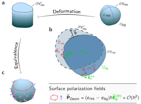
Figure 1: Overview of the PT framework and notations. a. A body (nanoresonator) is deformed with boundary changing from $\partial V_{\rm res}$ to $\partial V_{\rm res}^{\prime}$. b. Geometrical deformation is parameterized by $h(\mathbf{r}_{\scriptscriptstyle\partial V_{\rm res}})\hat{\mathbf{n}}$. c. The perturbed body is modeled as the unperturbed body dressed (augmented) by a surface-polarization distribution, $\widetilde{\mathbf{P}}_{\rm Geom}$ given by Eq. (1b). In b-c, $\widetilde{\mathbf{E}}^{\pm\scriptscriptstyle\delta[h]}\equiv\widetilde{\mathbf{E}}(\mathbf{r}_{\scriptscriptstyle\partial V_{\rm res}}\pm\delta[h])$ with $\delta[h]\equiv 0^{-}$ for $h>0$ and otherwise $\delta[h]\equiv 0^{+}$.

Figure 1 shows our notations. A body (nanoresonator) is deformed into a perturbed one with its boundary changing from $\partial V_{\rm res}$ to $\partial V{{}^{\prime}}_{\rm res}$. The deformation is parameterized by $h(\mathbf{r}_{\scriptscriptstyle\partial V_{\rm res}})\hat{\mathbf{n}}$ measuring perpendicular shift from $\partial V_{\rm res}$ to $\partial V_{\rm res}^{\prime}$, where $\hat{\mathbf{n}}$ denotes unit outward normal vector of $\partial V_{\rm res}$ and $\mathbf{r}_{\scriptscriptstyle\partial V_{\rm res}}$ denotes coordinates on $\partial V_{\rm res}$. The permittivity tensors of the nanoresonator and background are denoted by $\bm{\varepsilon}_{\rm res}$ and $\bm{\varepsilon}_{\rm bg}$, respectively. Outward ($h>0$) and inward ($h<0$) deformations result in material changes $\Delta\bm{\varepsilon}\equiv\bm{\varepsilon}_{\rm res}-\bm{\varepsilon}_{\rm bg}$ and $-\Delta\bm{\varepsilon}$, respectively, in perturbed domains denoted by ${\mathbb{P}}_{\rm res}$ and ${\mathbb{P}}_{\rm bg}$, respectively. The remaining unperturbed domain is denoted by ${\mathbb{U}}_{\rm res,bg}$ belonging either to the resonator (res) or background (bg).

Field Extrapolation in Perturbed Domains: We start from the Lippman–Schwinger integral equation expressing the electric fields of the perturbed modes, $\widetilde{\mathbf{E}}_{\rm p}$, with the Green’s tensor of the unperturbed system, ${\bf{\sf\displaystyle G}}_{\rm u}$: $\widetilde{\mathbf{E}}_{\rm p}(\mathbf{r})=\omega^{2}\int{\bf{\sf\displaystyle G}}_{\rm u}(\mathbf{r},\mathbf{r}^{\prime};\omega)f(\mathbf{r}^{\prime})\Delta\bm{\varepsilon}(\omega)\widetilde{\mathbf{E}}_{\rm p}(\mathbf{r}^{\prime})d^{3}\mathbf{r}^{\prime}$ See , where $f(\mathbf{r})$ is a filling function with values of $1$ and $\textnormal{-}1$ for $\mathbf{r}\in{\mathbb{P}}_{\rm res}$ and ${\mathbb{P}}_{\rm bg}$, respectively, and $0$ elsewhere.

To expand the perturbed modes $\widetilde{\mathbf{E}}_{{\rm p}}$ with a complete basis for both inward and outward deformations, we consider a set of unperturbed modes $\widetilde{\mathbf{E}}_{{\rm u}}$ composed of a subset of dominant QNMs and additional numerical modes Vial et al. (2014). Highly accurate reconstructions in this modal basis have been recently obtained for complex problems, involving noncompact shapes (e.g. resonator dimers) and nonuniform environments (e.g. metallic substrates) Yan et al. (2018), as well as gratings with their many inevitable branch cuts in the complex-frequency plane Gras et al. (2019). However, for shape deformations, directly expanding $\widetilde{\mathbf{E}}_{{\rm p}}$ into the $\widetilde{\mathbf{E}}_{{\rm u}}$ basis would lead to nonuniform convergence owing to field discontinuity across $\partial V_{\rm es}$, see Lai et al. (1990); Johnson et al. (2002). To bypass this issue in a systematic way, we here develop a novel extrapolation technique that allows us to consider large deformations. First, disregarding ${\mathbb{P}}_{\rm res,bg}$ domains, we perform the modal expansion in the ${\mathbb{U}}_{\rm res,bg}$ domains only, $\widetilde{\mathbf{E}}_{\rm p}(\mathbf{r})=\sum_{n}\alpha_{n}\widetilde{\mathbf{E}}_{{\rm u};n}(\mathbf{r})$, $\alpha_{n}$ being the expansion coefficient. Then, we take a key step and extrapolate $\widetilde{\mathbf{E}}_{\rm p}$ in $\mathbb{P}_{\rm res,bg}$ from fields in $\mathbb{U}_{\rm res,bg}$ with a Taylor expansion of $\widetilde{\mathbf{E}}_{\rm p}$ about $\partial V_{\rm res}$: $\widetilde{\mathbf{E}}_{\rm p}(\mathbf{r})=\sum_{j=0}^{\infty}(l^{j}/j!){\overrightarrow{\partial}}_{\hat{\mathbf{n}}}^{j}\widetilde{\mathbf{E}}_{\rm p}(\mathbf{r}_{\scriptscriptstyle\partial V_{\rm res}}+\delta[h]\hat{\mathbf{n}})$. Here $\delta[h]\equiv 0^{-}$ for $h>0$ and otherwise $\delta[h]\equiv 0^{+}$; $\mathbf{r}=l\hat{\mathbf{n}}+\mathbf{r}_{\scriptscriptstyle\partial V_{\rm res}}$ with $l\in[0,\,h]$; ${\overrightarrow{\partial}}_{\hat{\mathbf{n}}}^{j}f(\mathbf{r}_{\scriptscriptstyle\partial V_{\rm res}})\equiv(\hat{\mathbf{n}}\cdot{\bm{\nabla}})^{j}f(\mathbf{r}_{\scriptscriptstyle\partial V_{\rm res}})$. The Taylor expansion is justified because the materials in ${\mathbb{P}_{\rm res,bg}}$ are the same as in ${\mathbb{U}_{\rm res,bg}}$ and electric fields in uniform domains (without permittivity discontinuities) are analytic.

The volume-integral Lippman–Schwinger equation is then reformulated as a surface-integral equation over $\partial V_{\rm res}$ See :

$$\widetilde{\mathbf{E}}_{\rm p}(\mathbf{r}){=}{\oint_{\partial V_{\rm res}}}{\bf{\sf\displaystyle G}}_{\rm u}(\mathbf{r},\mathbf{r}_{\scriptscriptstyle\partial V_{\rm res}}{-}{\delta[h]}\hat{\mathbf{n}};\omega)\widetilde{\mathbf{P}}_{\rm Geom}(\mathbf{r}_{\scriptscriptstyle\partial V_{\rm res}})d^{2}\mathbf{r}_{\scriptscriptstyle\partial V_{\rm res}},$$ (1a)

with surface polarization $${\mathbf{P}}_{\rm Geom}$$ given by

$$\widetilde{\mathbf{P}}_{\rm Geom}(\mathbf{r}_{\scriptscriptstyle\partial V_{\rm res}})=\sum_{k=0}^{\infty}\sum_{j=0}^{\infty}{\overleftarrow{\partial}}_{\hat{\mathbf{n}}}^{\,\,k}\Delta\bm{\varepsilon}\,{\rm c}_{\scriptscriptstyle jk}{\overrightarrow{\partial}}_{\hat{\mathbf{n}}}^{j}\widetilde{\mathbf{E}}_{\rm p}(\mathbf{r}_{\scriptscriptstyle\partial V_{\rm res}}{+}{\delta[h]\hat{\mathbf{n}}}).$$ (1b)

Here $${\rm c}_{\scriptscriptstyle jk}=\frac{h^{k+j+1}}{k!j!}\left(\frac{1}{k+j+1}+\kappa_{\rm m}\frac{2h}{k+j+2}+\kappa_{\rm g}\frac{h^{2}}{k+j+3}\right) \kappa_{\rm m,g} \partial V_{\rm res} f(\mathbf{r}_{\scriptscriptstyle\partial V_{\rm res}}){\overleftarrow{\partial}}_{\hat{\mathbf{n}}}^{\,\,k}\equiv(\hat{\mathbf{n}}\cdot{\bm{\nabla}})^{k}f(\mathbf{r}_{\scriptscriptstyle\partial V_{\rm res}})$$ with denoting the mean and Gaussian curvatures of , respectively; .

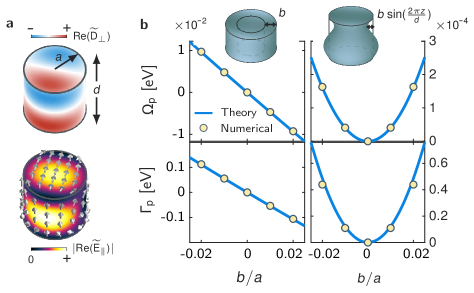
Figure 2: Validation of the perturbation theory for a silicon rod (radius $a=200\,\rm nm$, height $d=400\,\rm nm$ and permittivity $\varepsilon_{\rm si}=12.96$) in air. a. Field distribution of a (1,1,1) Mie’s mode on the rod surface. The QNM frequency is $\widetilde{\omega}_{\rm u}=0.74-0.034{\rm i}\,\rm eV$. (Top) Real part of perpendicular normalized displacement field; (bottom) amplitude of real part of (vectorial) parallel normalized electric fields. The arrows specify the field direction. b. Modal eigenfrequency shifts, $\Delta\widetilde{\omega}\equiv\Delta\widetilde{\Omega}-{\rm i}\Delta\widetilde{\Gamma}/2$, as the nanorod radius varies either uniformly (left, $h=b$) or sinusoidally [right, $h=b\sin(2\pi z/d)$]. The (left) linear and (right) quadratic dependencies of $\Delta\widetilde{\omega}$ on deformation parameter $b$ are accurately predicted using the first-order and second-order PTs, respectively.

Equations (1) are the cornerstone of our lately developed PT. They define a new integral formulation for electric fields of perturbed modes, which shall allow us to conveniently derive PT formulae to arbitrary orders.

Perturbation Theory: Injection the modal expansions of $\widetilde{\mathbf{E}}_{\rm p}$ and ${\bf{\sf\displaystyle G}}_{\rm u}$ Lalanne et al. (2018) in Eqs. (1), we obtain a linear eigenvalue equation for perturbed modes $\left\{\widetilde{\omega}_{\rm p},\ket{\bm{\alpha}}\equiv[\alpha_{1};\alpha_{2};\cdots]\right\}$ (Sec. S5 of  See ):

$${\bf\mathcal{H}}_{0}\ket{\bm{\alpha}}=\widetilde{\omega}_{\rm p}\left[{\bf{\sf\displaystyle I}}+{\bf\mathcal{H}}_{\rm p}\right]\ket{\bm{\alpha}}.$$ (2a)

Here $${\bf\mathcal{H}}_{0} {\bf{\sf\displaystyle I}} {\bf\mathcal{H}}_{\rm p}$$ is a diagonal matrix with diagonal elements being frequencies of unperturbed modes; denotes the identity matrix. accounts for the perturbation contribution, for which we make the first-order approximation

$${\mathcal{H}_{{\rm p};nm}\simeq\matrixelement{\left(\widetilde{\mathbf{E}}_{{\rm u};n}^{\rm bg}\right)^{*}}{h\Delta\bm{\varepsilon}(\widetilde{\omega}_{{\rm u};m})}{\widetilde{\mathbf{E}}_{{\rm u};m}^{\rm res}}_{\partial V_{\rm res}}},$$ (2b)

where $$\matrixelement{\left(\widetilde{\mathbf{E}}_{{\rm u};n}^{\rm bg}\right)^{*}}{h\Delta\bm{\varepsilon}(\widetilde{\omega}_{{\rm u};m})}{\widetilde{\mathbf{E}}_{{\rm u};m}^{\rm res}}_{\partial V_{\rm res}}{\equiv}\oint_{\partial V_{\rm res}}\widetilde{\mathbf{E}}_{{\rm u};n}(\mathbf{r}_{\scriptscriptstyle\partial V_{\rm res}}{+}{0^{+}}\hat{\mathbf{n}})\cdot{h(\mathbf{r}_{\scriptscriptstyle\partial V_{\rm res}})\Delta\bm{\varepsilon}(\widetilde{\omega}_{{\rm u};m})}\cdot\widetilde{\mathbf{E}}_{{\rm u};m}(\mathbf{r}_{\scriptscriptstyle\partial V_{\rm res}}{+}{0^{-}}\hat{\mathbf{n}})d^{2}\mathbf{r}_{\scriptscriptstyle\partial V_{\rm res}} \widetilde{\mathbf{E}}_{{\rm u};n}^{\rm bg} \widetilde{\mathbf{E}}_{{\rm u};n}^{\rm res} \widetilde{\mathbf{E}}_{{\rm u};n} \partial V_{\rm res}$$, and and denote at the outer and inner sides of , respectively.

Equations (2) constitute our first important result, a rigorous first-order PT for deformation problems of open systems. The essential difference with earlier works Muljarov and Langbein (2016a); Weiss et al. (2016) is the interplay of the inner and outer fields at the resonator boundary in the perturbation matrix ${\bf\mathcal{H}}_{\rm p}$. The interplay guaranties that for vanishing $h$, $\widetilde{\mathbf{E}}_{{\rm p};n}$ uniformly converges towards $\widetilde{\mathbf{E}}_{{\rm u};n}$ for all $n$—whereas earlier formalisms do so only nonuniformly, see Sec. S2 of See —, thereby allowing us to obtain accurate predictions for large deformations with a small number of retained QNMs. Accordingly, it is unnecessary to include numerical modes practically (at least for the first-order PT corrections). For small deformations, the first-order single-mode frequency shift, $\Delta\widetilde{\omega}_{n}\equiv\widetilde{\omega}_{{\rm p};n}-\widetilde{\omega}_{{\rm u};n}$, is given by

$$\Delta\widetilde{\omega}_{n}\simeq-\widetilde{\omega}_{{\rm u};n}\matrixelement{\left(\widetilde{\mathbf{E}}_{{\rm u};n}^{\rm bg}\right)^{*}}{h\Delta\bm{\varepsilon}(\widetilde{\omega}_{{\rm u};n})}{\widetilde{\mathbf{E}}_{{\rm u};n}^{\rm res}}_{\partial V_{\rm res}},$$ (3)

which is consistent with earlier works on normal-mode PTs Johnson et al. (2002)—in the limit of ${\rm Im}(\widetilde{\omega}_{{\rm u};n})\to 0$ and ${\rm Im}(\widetilde{\mathbf{E}}_{{\rm u};n})\to 0$— and QNM PTs using the LFC for tiny deformations Lai et al. (1990); Yang et al. (2015).

Validation: We consider a silicon rod in air that supports Mie’s resonances indexed by $(q,n,l)$—the azimuthal, radial and longitudinal numbers. Figure 2a shows the field distribution of a $(1,1,1)$ mode, which is selected for the following study. In this initial study aiming at the validation of the first-order PT of Eq. (2), the rod is only slightly deformed by a uniform radial change $h=b$. The left panel in Fig. 2b compares the values of $\Delta\widetilde{\omega}$ predicted from Eq. (3) with exact numerical data obtained with the QNMEig solver of the freeware MAN (Modal Analysis of Nanoresonators) Yan et al. (2018); Lalanne (2020) implemented with COMSOL Multiphysics. The quantitative agreement, along with similar observations in Figs. S2-S3 See , evidences the soundness of Eq. (3) in the limit of vanishing perturbations.

The first-order PT can be generalized to high-order ones by retaining high-order terms in ${\bf\mathcal{H}}_{\rm p}$ when solving the eigenvalue problem of Eq. (2a). As an example to validate our theory at high order, we consider another radial deformation $h=b\sin(2\pi z/d)$, where $z$ denotes the longitudinal coordinate. In this case, the first-order correction vanishes since $h$ is odd with respect to $z$, and the second-order correction is dominant. As evidenced in the right panel of Fig. 2b and also in Figs. S4 and S5 See , the second-order PT accurately predicts the quadratic frequency shift $\Delta\widetilde{\omega}$ of the $(1,1,1)$ mode, with a residual error due to modal truncation . Compared to first-order results, the accuracy improvement is obvious. However, the second-order PT requires a much larger number of modes to reach the accuracy. Balancing between accuracy and effectiveness suggests us to use the first-order PT for the following studies.

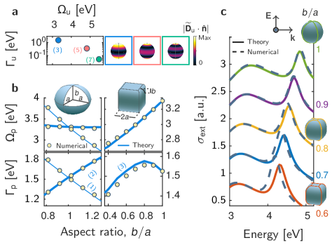
Figure 3: Test for large deformations of a silver sphere (50-nm radius) in air. Two deformations, into spheroids or cuboids, are considered. Silver is modelled by a Drude permittivity $\varepsilon_{\rm Ag}=1-\omega_{p}^{2}/(\omega^{2}+i\omega\gamma)$ with $\hbar\omega_{p}=9$ eV and $\hbar\gamma=0.021$ eV. a. (Left) Eigenfrequencies $\widetilde{\omega}_{\rm u}\equiv\Omega_{\rm u}-i\Gamma_{\rm u}/2$ of dipole (blue) and quadrupole (red) QNMs. Degeneracy factors are given in parenthesis. (Right) Amplitudes of perpendicular normalized electric displacement fields for dipole, quadrupole and hexapole QNMs with azimuthal order $m=0$. b. Eigenfrequencies $\widetilde{\omega}_{\rm p}\equiv\Omega_{\rm p}-i\Gamma_{\rm p}/2$ of perturbed dipole QNMs for spheroids and cuboids as aspect ratios $b/a$ vary (for small deformations, $b/a\simeq 1$). c. Extinction-cross-section spectra of cuboids for several values of $b/a$. $2\times 15$ QNMs are used in b-c; additional static QNMs at zero frequency are taken into account in $\bf c$.

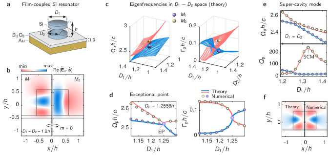
Figure 4: Application of the PT for designing exceptional point (EP) and high-$Q$ super-cavity mode (SCM). a. A Si dumbbell-shaped nanoresonator sits on an Au substrate coated with a 50-nm-thick $\text{SiO}_{2}$ layer. The dumbbell consists of three equal-high cylinders (total height $h=500\,\rm nm$) with diameters $D_{1}$, $D_{2}$ and $D_{1}$ (from top to bottom). The Au permittivity is approximated by the Lorentz-Drude model $\varepsilon_{\rm Au}(\omega)=\varepsilon_{\infty}-\omega_{p,1}^{2}/(\omega^{2}+i\gamma_{1}\omega)-\omega_{p,2}^{2}/(\omega^{2}-\omega_{0}^{2}+i\gamma_{2}\omega)$ with $\varepsilon_{\infty}=6$, $\hbar\omega_{p,1}=8.67\,\rm eV$, $\hbar\gamma_{1}=0.1\,\rm eV$, $\hbar\omega_{p,2}=3.65\,\rm eV$, $\hbar\gamma_{2}=2.15\,\rm eV$, $\hbar\omega_{0}=7.38\,\rm eV$. b. Field distributions of azimuthal-component electric fields, ${\rm Re}\left(\widetilde{E}_{\rm u;\phi}\right)$, of two modes $M_{1}$ and $M_{2}$ with azimuthal order $m=0$ obtained for $D_{1}=D_{2}=1.2h$. c. Eigenfrequencies calculated with Eqs. (2) for perturbed QNMs resulting from $M_{1}-M_{2}$ coupling as the parameter space ($D_{1}-D_{2}$) is spanned. d. Eigenfrequencies for $D_{2}=1.2558h$. The EP is labelled. e. Resonance frequencies and quality factors for $D_{1}=D_{2}$. The SCM with $Q_{\rm p}\simeq 240$ is labelled in the lower panel. f. SCM-field distribution ${\rm Re}\left(\widetilde{E}_{\rm p;\phi}\right)$.

Reconstruction of scattered fields: The use of the frequency shift formula of Eqs. (2) or  (3) for designing nanoresonators with tailored resonance wavelengths or quality factors will be discussed later. In inverse design, the possibility of predicting the nanoresonator response with unperturbed modes is equally useful Jensen and Sigmund (2011); Molesky et al. (2018); Miller (2012). Thus we consider a perturbed nanoresonator driven by an incident field ${\mathbf{E}}_{\rm in}$ and denote by ${\mathbf{E}}_{\rm sca}$ the scattered field. By taking into account volume polarization $\Delta\bm{\varepsilon}{\mathbf{E}}_{\rm in}$ due to the incident field, Eqs. (1) is generalized: ${\mathbf{E}}_{\rm sca}(\mathbf{r})=\int_{V_{\rm res}}{\bf{\sf\displaystyle G}}_{\rm u}(\mathbf{r},\mathbf{r}^{\prime};\omega)\Delta\bm{\varepsilon}(\omega){\mathbf{E}}_{\rm in}(\mathbf{r}^{\prime})d^{3}\mathbf{r}^{\prime}+\oint_{\partial V_{\rm res}}{\bf{\sf\displaystyle G}}_{\rm u}(\mathbf{r},\mathbf{r}_{\scriptscriptstyle\partial V_{\rm res}}^{\prime}-\delta\hat{\mathbf{n}};\omega){\mathbf{P}}_{\rm Geom}(\mathbf{r}_{\scriptscriptstyle\partial V_{\rm res}}^{\prime})d^{2}\mathbf{r}_{\scriptscriptstyle\partial V_{\rm res}}^{\prime}$ (see Sec. S8 of  See ) where ${\mathbf{P}}_{\rm Geom}$ is expressed with Eq. (1b) using the total field ${\mathbf{E}}_{\rm in}+{\mathbf{E}}_{\rm sca}$. By expanding ${\mathbf{E}}_{\rm sca}$ with unperturbed modes, ${\mathbf{E}}_{\rm sca}=\sum_{n}\beta_{n}\widetilde{\mathbf{E}}_{{\rm u};n}$, and performing the modal expansion for ${\bf{\sf\displaystyle G}}_{\rm u}$, we obtain a linear equation for $\ket{\bm{\beta}}\equiv[\beta_{1};\beta_{2};\cdots]$:

$${\bf\mathcal{H}}_{0}\ket{\bm{\beta}}=\omega\left[{\bf{\sf\displaystyle I}}+{\bf\mathcal{H}}_{\rm p}\right]\ket{\bm{\beta}}+\omega\left[\ket{\bm{B}}+\ket{\bm{S}}\right],$$ (4)

where the source terms $\ket{\bm{B}}\equiv[B_{1};B_{2};\cdots]$ and $\ket{\bm{S}}\equiv[S_{1};S_{2};\cdots]$ with $B_{n}=\int_{V_{\rm res}}\widetilde{\mathbf{E}}_{{\rm u};n}(\mathbf{r})\Delta\bm{\varepsilon}(\widetilde{\omega}_{n}){\mathbf{E}}_{\rm in}(\mathbf{r})d^{3}\mathbf{r}$ and $S_{n}=\matrixelement{\left(\widetilde{\mathbf{E}}_{{\rm u};n}^{\rm bg}\right)^{*}}{h\bm{\Delta}\varepsilon(\widetilde{\omega}_{n})}{{\mathbf{E}}_{\rm in}}_{\scriptscriptstyle\partial V_{\rm res}}$. Note that, for ${\mathbf{E}}_{\rm in}=0$ ($\ket{\bm{S}}=\ket{\bm{B}}=0$), Eq. (4) reduces to the eigenvalue equation for perturbed modes; when the perturbation vanishes (${\bf\mathcal{H}}_{\rm p}=0$ and $\ket{\bm{S}}=0$), $\ket{\bm{\beta}}$’s become modal excitation coefficients of the unperturbed nanoresonator. Equation (4) allows us to reconstruct optical responses of perturbed nanoresonators and constitutes the second main result of this letter.

Application: When performing inverse design of a photonic device, one explores a large parameter space to optimize several electromagnetic observables with typically gradient based algorithms through repeated simulations of Maxwell’s equations. The developed PT offers new opportunities for geometrical optimization. First, QNM expansions make the physics transparent, thereby helping the interpretation of optimized results. Second, the computational cost of problems involving broad bandwidth, multi-frequency bands or multi-illumination instances can be dramatically reduced Lalanne et al. (2018), benefiting from the analyticity of objective functions. Third, since nanoresonator responses are generally driven by a few QNMs, the optimization problem in large parameter space becomes more tractable Molesky et al. (2018); Wu et al. (2020), and the expensive task of computing gradients, with either finite schemes or the adjoint method, is simplified due to small-dimensional matrix problems of Eqs. (2) or (4). How far these equations may allow us to accurately explore parameter space—before being obliged to locally restabilize the optimization by computing again a few dominant QNMs—decisively impact the effectiveness of the present PT.

To quantify the exploration capability of Eqs. (2) that take into account deformation-induced couplings between different modes, we consider large spheroidal and cuboidal deformations of a silver sphere. The results are summarized in Fig. 3. For solving Eq. (2), 15 modes—whose frequencies and modal profiles are shown in Fig. 3a—plus their 15 complex conjugated counterparts $\left\{-\widetilde{\omega}_{{\rm u};n}^{*},\widetilde{\mathbf{E}}_{{\rm u};n}^{*}\right\}$ are considered, thereby giving a $30\times 30$ ${\bf\mathcal{H}}_{\rm p}$ matrix. Figure 3b compares the theoretical predictions of the fundamental-dipole-QNM frequencies of the deformed geometries with the numerical data. Note that, for spheroids, the original dipole triplet is split into a doublet and a singlet. An overall quantitative agreement, up to deformations with 30%-50% volume changes, is achieved. This level of accuracy for large deformations, using a few QNMs, is largely unattainable with available cavity QNM Muljarov et al. (2010); Weiss et al. (2016) or normal-mode PTs  Johnson et al. (2002) (see the comparisons in Fig. S1 See ). In Fig. 3c, we additionally compare the theoretical predictions of Eq. (4) for the extinction-cross-section spectra of cuboids with exact numerical results obtained with the boundary element method, showing again quantitative agreement. More numerical evidences are shown in Figs. S6-9 See .

We further exemplify the potential of the present PT for inverse design by designing super-cavity modes (SCMs) and exceptional points (EPs) (a general workflow of employing the PT for inverse design is detailed in Sec. S9 of  See ). SCMs, the analogues of bound states in the continuum for finite-size structures, offer high $Q$’s owing to destructive radiation interferences Rybin et al. (2017), while EPs with two or more coalescing states have implications for lasing Wong et al. (2014) and sensing Chen et al. (2017) applications. Hereafter, we consider a complex geometry, a Si dumbbell-shaped resonator deposited on an Au substrate coated with a thin ${\rm Si}{\rm O}_{2}$ film. Since SCMs and EPs can be constructed with a bi-mode coupled system by carefully tuning modal coupling constants, we restrict the parameter space to two diameters, $D_{1}$ and $D_{2}$ (see Fig. 4a). The design begins with a guessed geometry, $D_{1}=D_{2}=600\,\rm nm$ and $h=500\,\rm nm$ (height), for which we compute the QNMs with the solver QNMEig Yan et al. (2018). We further select two QNMs, denoted by $M_{1}$ and $M_{2}$—that are frequency-protected from others, i.e., $|\widetilde{\omega}_{{\rm u};n}-\widetilde{\omega}_{{\rm u};M_{i}}|\gg|{\bf\mathcal{H}}_{{\rm p};nM_{i}}|$ for $n\notin\left\{M_{1},M_{2}\right\}$—, thereby defining an isolated bi-mode coupled system. Figure 4b shows the modal profiles of $M_{1,2}$ with azimuthal order $m=0$. Now, the calculation of the perturbed QNMs with Eqs. (2) amounts to solve a simple $2\times 2$ eigenmatrix. As shown with Fig. 4c, we can directly and straightforwardly explore the entire parameter space with Eqs. (2), without requiring any further time-consuming full-wave computations of the QNMs.

An EP is obtained for $D_{2}=1.2558\,h$ when the two eigenvalues coalesce as $D_{1}$ is varied, see details in Fig. 4d. On the other hand, the design of SCMs, revealed by their high-$Q$ values, does not necessitate a shape optimization as precise as that for EPs. For instance, constraining $D_{1}=D_{2}$, we observe in Fig. 4e that $Q_{\rm p}$ of one mode is significantly increased for $D_{1}=650\,\rm nm$, identifying a SCM with a 20-fold $Q$ enhancement (see Fig. 4f for the mode profiles). Again, no need for further iterative full-wave computations; the SCM is directly found by exploring the parameter space with Eq. (2). Additionally note the quantitative agreement between the theoretical predictions and full-wave numerical data; and, accordingly, further optimization iterations are thus unnecessary.

Conclusions: The present PT establishes a general and rigorous framework for predicting the optical responses of largely deformed resonators from the sole knowledge of the initial unperturbed modes. There is, in principle, no restriction on the resonator geometry and constitutive materials. It offers unprecedented numerical efficiency and physical transparency, making it a good tool for nanoresonator design.

Acknowledgements—This project was supported by the National Key Research and Development Program of China (2017YFA0205700), the National Natural Science Foundation of China (61927820).

References

- Novotny (2012) L. Novotny, Principles of Nano-Optics (Cambridge University Press, Cambridge, 2012).
- Lalanne et al. (2018) P. Lalanne, W. Yan, V. Kevin, C. Sauvan, and J.-P. Hugonin, Laser Photonics Rev. 4, 1700113 (2018).
- Jensen and Sigmund (2011) J. S. Jensen and O. Sigmund, Laser Photon. Rev. 5, 308 (2011).
- Molesky et al. (2018) S. Molesky, Z. Lin, A. Y. Piggott, W. Jin, J. Vucković, and A. W. Rodriguez, Nat. Photonics 12, 659 (2018).
- Kato (1972) T. Kato, Perturbation theory for linear operators (Springer Science & Business Media, Berlin, 1972).
- Harrington (1961) R. F. Harrington, Time Harmonic Electromagnetic Fields (McGraw-Hill, New York, 1961).
- Johnson et al. (2002) S. G. Johnson, M. Ibanescu, M. A. Skorobogatiy, O. Weisberg, and J. Joannopoulos, Phys. Rev. E 65, 066611 (2002).
- Yang et al. (2015) J. Yang, H. Giessen, and P. Lalanne, Nano Lett. 15, 3439 (2015).
- (9) See Supplemental Material for comparisons with other existing PTs, derivation details of the first- and second- order PTs and reconstructing optical responses under external stimuli, and further discussions of exploiting the PT in inverse design, which includes Refs. Harrington (1961); Klein et al. (1993); Yang et al. (2015); Weiss et al. (2016); Cognée et al. (2019); Leung et al. (1994); Lee et al. (1999); Muljarov et al. (2010); Muljarov and Langbein (2016a); Lalanne et al. (2018); Johnson et al. (2002); Vial et al. (2014); Yan et al. (2018); Muljarov and Langbein (2016b).
- Note (1) For a review of the impact of non-Hermiticity on first-order cavity PT and other related physical phenomena, e.g. Purcell effects, please refer to Lalanne et al. (2018).
- Leung et al. (1994) P. Leung, S. Liu, and K. Young, Phys. Rev. A 49, 3982 (1994).
- Lee et al. (1999) K. Lee, P. Leung, and K. Pang, J. Opt. Soc. Am. B 16, 1418 (1999).
- Muljarov and Langbein (2016a) E. A. Muljarov and W. Langbein, Phys. Rev. B 93, 075417 (2016a).
- Weiss et al. (2016) T. Weiss, M. Mesch, M. Schäferling, H. Giessen, W. Langbein, and E. A. Mulfarov, Phys. Rev. Lett. 116, 237401 (2016).
- Lai et al. (1990) H. Lai, P. Leung, K. Young, P. Barber, and S. Hill, Phys. Rev. A 41, 5187 (1990).
- Vial et al. (2014) B. Vial, A. Nicolet, F. Zolla, and M. Commandré, Phys. Rev. A 89, 023829 (2014).
- Yan et al. (2018) W. Yan, R. Faggiani, and P. Lalanne, Phys. Rev. B 97, 205422 (2018).
- Miller et al. (2014) O. Miller, C. Hsu, M. T. H. Reid, W. Qiu, B. Delacy, J. Joannopoulos, M. Soljačić, and S. Johnson, Phys. Rev. Lett. 112, 123903 (2014).
- Wu et al. (2020) T. Wu, A. Baron, P. Lalanne, and K. Vynck, Phys. Rev. A 101, 011803(R) (2020).
- Gras et al. (2019) A. Gras, W. Yan, and P. Lalanne, Opt. Lett. 44, 3494 (2019).
- Lalanne (2020) P. Lalanne, Man (modal analysis of nanoresonators), https://zenodo.org/record/3631242#.XqD5CMgzY2x (2020).
- Note (2) The computation of with the second-order PT includes modes with .
- Miller (2012) O. D. Miller, Photonic design: from fundamental solar cell physics to computational inverse deisgn (2012), ph.D. thesis.
- Muljarov et al. (2010) E. A. Muljarov, W. Langbein, and R. Zimmermann, Europhys. Lett. 92, 50010 (2010).
- Rybin et al. (2017) M. Rybin, K. Koshelev, Z. Sadrieva, K. Samusev, A. Bogdanov, M. Limonov, and Y. Kivshar, Phys. Rev. Lett. 119, 243901 (2017).
- Wong et al. (2014) F. Wong, Z. Ma, R. Wang, and X. Zhang, Science 346, 972–975 (2014).
- Chen et al. (2017) W. Chen, S. Özdemir, G. Zhao, J. Wiersig, and L. Yang, Nature 448, 192–196 (2017).
- Klein et al. (1993) O. Klein, D. Dressel, and G. Gr’́uner, Int. J. Infrared Milli. Waves 14, 2423 (1993).
- Cognée et al. (2019) K. G. Cognée, W. Yan, F. L. China, D. Balestri, F. Intonti, M. Gurioli, A. F. Koenderink, and P. Lalanne, Optica 6, 269 (2019).
- Muljarov and Langbein (2016b) E. A. Muljarov and W. Langbein, Phys. Rev. B 94, 235438 (2016b).