Form Factors and Decay of $\bar{B}_{s}^{0}\to J/\psi\phi$ From QCD Sum Rule

Abstract

We calculate $\bar{B}_{s}^{0}\to\phi$ translation form factors $V$, $A_{0}$, $A_{1}$, $A_{2}$ based on QCD sum rule and study the nonleptonic two-body decay of $\bar{B}_{s}^{0}\to J/\psi\phi$ with the form factors obtained. We calculate the time-integrated branching ratio of $\bar{B}_{s}^{0}\to J/\psi\phi$ decay. The results for both the total branching ratio and the cases for the final vectors in longitudinal and transverse polarizations are consistent with experimental data.

I Introduction

$CP$ asymmetry arises due to the non-vanishing complex phase of the Cabibbo-Kobayashi-Maskawa (CKM) matrix elements KM ; Cabibbo in the standard model (SM). The requirement of unitarity of the CKM matrix results in a set of triangles in the complex plane. $\bar{B}_{s}^{0}(t)\to J/\psi\phi$ is a golden decay mode to measure the angle $\beta_{s}$, one of the angles of the triangle in the $bs$ sector: $V_{us}V_{ub}^{*}+V_{cs}V_{cb}^{*}+V_{ts}V_{tb}^{*}=0$. The angle $\beta_{s}$ is related to the sides of unitarity triangle by $\beta_{s}=arg[-V_{ts}V_{tb}^{*}/(V_{cs}V_{cb}^{*})$ R17 . $\bar{B}_{s}(t)\to J/\psi\phi$ decay stimulate wide interest in both theory and experiment MA2016 ; CMS1 ; Lei2010 ; Colan2011 ; Liu2014 . This decay mode is not only interesting for analysis of $CP$ violation, but also useful for studying strong interaction in the decay process. Factorization is a basic method to calculate non-leptonic $B$ meson decays, where it is assumed that the hadronic decay amplitude can be factorized as a product of matrix elements of two local quark-antiquark currents Fak1978 ; Cab1978-1 . The QCD non-factorizable corrections to the factorization result can be calculated systematically in perturbation theory, which is called QCD factorization Ben1999 ; Ben2000 . The hadronic matrix element of the quark-antiquark current in $B$ decays can be decomposed as polynomials of form factors. The form factors are in general non-perturbative quantities in QCD, which can be calculated with non-perturbative method, such as Lattice QCD, QCD sum rule, QCD light-cone sum rule, and quark model, etc. The $\bar{B}^{0}_{s}\to\phi$ transition form factors involved in $\bar{B}_{s}^{0}\to J/\psi\phi$ decay have been calculated by QCD light-cone sum rule (LCSR) Ball1998 ; R11 , Quark model (QM) R12 , and QCD sum rule R15 in literature. Some form factors obtained by QCD sum rule in Ref. R15 are different from other results calculated in Refs. R11 ; R12 by a sign. Here in this work, we revisit the $\bar{B}^{0}_{s}\to\phi$ transition form factors with QCD sum rule method. Then the from factors obtained in this work are used to study the nonleptonic decay of $\bar{B}_{s}^{0}\to J/\psi\phi$. The the transverse, longitudinal and total time-dependent decay widths $\Gamma_{L}(t)$, $\Gamma_{T}(t)$ and $\Gamma(t)$ are calculated respectively. The results are consistent with experimental data within experimental and theoretical uncertainties.

The remainder of this paper is organized as follows: In sec. II, we present the method to calculate the form factors in QCD sum rule method. Section III is for the numerical analysis, and Section IV for the application of the form factors in the decay mode $\bar{B}_{s}^{0}\to J/\psi\phi$. Section V is a brief summary.

II Theoretical Framework

1. The method

In the factorization approach, one ingredient of the amplitude of the decay mode $\bar{B}_{s}^{0}\to J/\psi\phi$ is the hadronic matrix element $\langle\phi|\bar{s}\gamma_{\nu}(1-\gamma_{5})b|\bar{B}_{s}^{0}\rangle$, which can be decomposed as

$$\langle\phi(\varepsilon,p_{2})|\bar{s}\gamma_{\nu}(1-\gamma_{5})b|\bar{B}_{s}^{0}(p_{1})\rangle = \varepsilon_{\nu\rho\alpha\beta}\varepsilon^{*\rho}p_{1}^{\alpha}p_{2}^{\beta}\frac{2V(q^{2})}{m_{B_{s}}+m_{\phi}}$$

$$-i(\varepsilon^{*}_{\nu}-\frac{\varepsilon^{*}\cdot q}{q^{2}}q_{\nu})(m_{B_{s}}+m_{\phi})A_{1}(q^{2})$$

$$+i[(p_{1}+p_{2})_{\nu}-\frac{m_{B_{s}}^{2}-m_{\phi}^{2}}{q^{2}}q_{\nu}]\varepsilon^{*}\cdot q\frac{A_{2}(q^{2})}{m_{B_{s}}+m_{\phi}}$$

$$-i\frac{2m_{\phi}\varepsilon^{*}\cdot q}{q^{2}}q_{\nu}A_{0}(q^{2}),$$

where the parameters $V$, $A_{0}$, $A_{1}$, $A_{2}$ are the transition form factors, and $q=p_{1}-p_{2}$.

The QCD sum rule method was originally developed by Shifman, Vainshtein and Zakharov in the late 1970s SVZ1 ; SVZ2 , which was widely used in hadronic process, see Ref. Colan2000 for a review. In order to calculate the transition form factors of $\bar{B}^{0}_{s}$ to $\phi$ in QCD, we consider the three-point correlation function defined by

$$\Pi_{\mu\nu}=i^{2}\int d^{4}xd^{4}ye^{ip_{2}\cdot x-ip_{1}\cdot y}\langle 0|T\{j^{\phi}_{\mu}(x)j_{\nu}(0)j_{5}(y)\}|0\rangle,$$ (2)

where the three currents are: (1) $j_{5}(y)=\bar{b}(y)i\gamma_{5}s(y)$, the current of $\bar{B}_{s}^{0}$ channel; (2) $j_{\nu}(0)=\bar{s}\gamma_{\nu}(1-\gamma_{5})b$, the current of weak transition; (3) $j_{\mu}^{\phi}(x)=\bar{s}(x)\gamma_{\mu}s(x)$, the current of $\phi$ channel.

One can use the double dispersion relation to express the correlation function as

$$\Pi_{\mu\nu}=\int ds_{1}ds_{2}\frac{\rho(s_{1},s_{2},q^{2})}{(s_{1}-p_{1}^{2})(s_{2}-p_{2}^{2})},$$ (3)

where $\rho(s_{1},s_{2},q^{2})$ is the spectral density. By inserting a full set of intermediate hadronic states into the time-ordered product in the correlation function, one can obtain the spectral density function as

$$\rho(s_{1},s_{2},q^{2})=\sum_{X}\sum_{Y}\langle 0|j_{\mu}^{\phi}|X\rangle\langle X|j_{\nu}|Y\rangle\langle Y|j_{5}|0\rangle\delta(s_{1}-m_{Y}^{2})\delta(s_{2}-m_{X}^{2})\theta(p_{X}^{0})\theta(p_{Y}^{0}),$$ (4)

where $X$ and $Y$ denote the full set of hadronic states of $\phi$ and $\bar{B}^{0}_{s}$ channels, respectively. Substituting the spectral density $\rho(s_{1},s_{2},q^{2})$ in Eq. (4) into Eq. (3) and integrating over $s_{1}$ and $s_{2}$, then we can get

$$\Pi_{\mu\nu}=\sum_{X}\sum_{Y}\frac{\langle 0|j_{\mu}^{\phi}|X\rangle\langle X|j_{\nu}|Y\rangle\langle Y|j_{5}|0\rangle}{(m_{Y}^{2}-p_{1}^{2})(m_{X}^{2}-p_{2}^{2})}+\mbox{\small{continuum states}}.$$ (5)

The result of the correlation function in the above equation can be also expressed as a sum of the ground states, excited states and continuum states

$$\Pi_{\mu\nu}=\frac{\langle 0|j_{\mu}^{\phi}|\phi\rangle\langle\phi|j_{\nu}|\bar{B}_{s}^{0}\rangle\langle\bar{B}_{s}^{0}|j_{5}|0\rangle}{(m_{B_{s}}^{2}-p_{1}^{2})(m_{\phi}^{2}-p_{2}^{2})}+\mbox{\small{excited states~{}+~{}continuum states}}.$$ (6)

Using the definition of decay constants in the following

$$\langle 0|\bar{s}\gamma_{\mu}s|\phi\rangle=m_{\phi}f_{\phi}\varepsilon_{\mu}^{(\lambda)},$$

$$\langle 0|\bar{s}\gamma_{\mu}\gamma_{5}s|\phi\rangle=0,$$

$$\langle 0|\bar{s}i\gamma_{5}b|\bar{B}_{s}^{0}\rangle=\frac{f_{B_{s}}m_{B_{s}}^{2}}{m_{b}+m_{s}},$$ (7)

where $f_{\phi}$ and $f_{B_{s}}$ are decay constants of the relevant mesons, the correlation function is changed to be

$$\Pi_{\mu\nu}=\frac{m_{\phi}f_{\phi}\varepsilon_{\mu}^{(\lambda)}\langle\phi(\varepsilon_{\mu}^{(\lambda)},p_{2})|j_{\nu}|\bar{B}_{s}^{0}(p_{1})\rangle f_{B_{s}}m_{B_{s}}^{2}}{(m_{B_{s}}^{2}-p_{1}^{2})(m_{\phi}^{2}-p_{2}^{2})(m_{b}+m_{s})}$$

$$+\mbox{\small{excited and continuum states}}.$$ (8)

Meanwhile the time-ordered current operator in the correlation function in Eq. (2) can be expanded in terms of a series of local operators with increasing dimensions in QCD

$$i^{2}\int d^{4}xd^{4}ye^{ip_{2}\cdot x-ip_{1}\cdot y}T\{j^{\phi}_{\mu}(x)j_{\nu}(0)j_{5}(y)\}$$ (9)

$$= C_{0\mu\nu}I+C_{3\mu\nu}\bar{\Psi}\Psi+C_{4\mu\nu}G^{a}_{\alpha\beta}G^{a\alpha\beta}+C_{5\mu\nu}\bar{\Psi}\sigma_{\alpha\beta}T^{a}G^{a\alpha\beta}\Psi$$

$$~{}+ C_{6\mu\nu}\bar{\Psi}\Gamma\Psi\bar{\Psi}\Gamma^{\prime}\Psi+\cdots,$$

where $C_{i\mu\nu}$ are Wilson coefficients, $I$ the unit operator, $\bar{\Psi}\Psi$ the local fermion field operator of light quarks, $G^{a}_{\alpha\beta}$ gluon strength tensor, $\Gamma$ and $\Gamma^{\prime}$ the matrices appearing in the procedure of calculating the Wilson coefficients. At deep negative values of $p_{1}^{2}$ and $p_{2}^{2}$, the Wilson coefficients can be calculated reliably in perturbative QCD, and the operator-product expansion (OPE) in Eq. (9) can converge quickly.

Considering the non-vanishing vacuum-expectation-value of the operators in Eq. (9), we can get the correlation function in terms of Wilson coefficients and condensates of local operators

$$\Pi_{\mu\nu} = i^{2}\int d^{4}xd^{4}ye^{ip_{2}\cdot x-ip_{1}\cdot y}\langle 0|T\{j^{\phi}_{\mu}(x)j_{\nu}(0)j_{5}(y)\}|0\rangle$$ (10)

$$= C_{0\mu\nu}I+C_{3\mu\nu}\langle 0|\bar{\Psi}\Psi|0\rangle+C_{4\mu\nu}\langle 0|G^{a}_{\alpha\beta}G^{a\alpha\beta}|0\rangle+C_{5\mu\nu}\langle 0|\bar{\Psi}\sigma_{\alpha\beta}T^{a}G^{a\alpha\beta}\Psi|0\rangle$$

$$~{}+ C_{6\mu\nu}\langle 0|\bar{\Psi}\Gamma\Psi\bar{\Psi}\Gamma^{\prime}\Psi|0\rangle+\cdots,$$

According to the Lorentz structure of the correlation function, Eq. (10) can be re-expressed by six parts

$$\Pi_{\mu\nu}=f_{0}\varepsilon_{\mu\nu\alpha\beta}p_{1}^{\alpha}p_{2}^{\beta}-i(f_{1}p_{1\mu}p_{1\nu}+f_{2}p_{2\mu}p_{2\nu}+f_{3}p_{1\mu}p_{2\nu}+f_{4}p_{1\nu}p_{2\mu}+f_{5}g_{\mu\nu}).$$ (11)

The coefficients $f_{i}$’s are consisted of perturbative and condensate contributions,

$$f_{i}=f_{i}^{pert}+f_{i}^{(3)}+f_{i}^{(4)}+f_{i}^{(5)}+f_{i}^{(6)}+\cdots,$$ (12)

where $f_{i}^{pert}$ is the perturbative contribution of the unit operator, and $f_{i}^{(3)}$, $f_{i}^{(4)}$, $f_{i}^{(5)}$, $f_{i}^{(6)}$, $\cdots$, are contributions of condensates of operators with increasing dimension in OPE.

In next section we shall know that perturbative contribution and gluon-condensate contribution can be written in the form of dispersion integration

$$f_{i}^{pert} = \int ds_{1}ds_{2}\frac{\rho^{pert}_{i}(s_{1},s_{2},q^{2})}{(s_{1}-p_{1}^{2})(s_{2}-p_{2}^{2})},$$

$$f_{i}^{(4)} = \int ds_{1}ds_{2}\frac{\rho^{(4)}_{i}(s_{1},s_{2},q^{2})}{(s_{1}-p_{1}^{2})(s_{2}-p_{2}^{2})}.$$

We can approximate the contribution of excited states and continuum states as integrations over some thresholds $s_{1}^{0}$ and $s_{2}^{0}$ in the above two equations. Then equating the two expressions of the correlation function in Eq. (8) and (11), we can get an equation for extracting the form factors. But such an equation may heavily depend on the approximation for the contribution of excited states and the contributions of higher dimensional operators in OPE. To improve such an equation and make the contribution of higher dimensional operator small, one can make Borel transformation over $p_{1}^{2}$ and $p_{2}^{2}$ in both sides, which can suppress the contributions of excited states and condensate of higher dimensional operators. The definition of Borel transformation to any function $f(x^{2})$ is

$$\hat{B}_{\left|\frac{}{}\right.x^{2},M^{2}}f(x^{2})=\lim_{\small\begin{array}[]{ll}&k\to\infty,x^{2}\to-\infty\\ &-x^{2}/k=M^{2}\end{array}}\frac{(-x^{2})^{k}}{(k-1)!}\frac{\partial^{k}}{\partial(x^{2})^{k}}f(x^{2}).$$

Matching these two expressions of the correlation function in Eq. (8) and (11), and performing Borel transformation for both variables $p_{1}^{2}$ and $p_{2}^{2}$, the sum rules for the form factors can be obtained

$$V(q^{2}) = -\frac{(m_{b}+m_{s})(m_{B_{s}}+m_{\phi})}{2m_{\phi}f_{\phi}f_{B_{s}}m_{B_{s}}^{2}}e^{m_{B_{s}}^{2}/M_{1}^{2}}e^{m_{\phi}^{2}/M_{2}^{2}}M_{1}^{2}M_{2}^{2}\hat{B}f_{0},$$

$$A_{1}(q^{2}) = -\frac{(m_{b}+m_{s})}{m_{\phi}f_{\phi}f_{B_{s}}m_{B_{s}}^{2}(m_{B_{s}}+m_{\phi})}e^{m_{B_{s}}^{2}/M_{1}^{2}}e^{m_{\phi}^{2}/M_{2}^{2}}M_{1}^{2}M_{2}^{2}\hat{B}f_{5},$$

$$A_{2}(q^{2}) = \frac{(m_{b}+m_{s})(m_{B_{s}}+m_{\phi})}{m_{\phi}f_{\phi}f_{B_{s}}m_{B_{s}}^{2}}e^{m_{B_{s}}^{2}/M_{1}^{2}}e^{m_{\phi}^{2}/M_{2}^{2}}M_{1}^{2}M_{2}^{2}\frac{1}{2}\hat{B}(f_{1}+f_{3}),$$ (13)

$$A_{0}(q^{2}) = -\frac{(m_{b}+m_{s})}{2m_{\phi}^{2}f_{\phi}f_{B_{s}}m_{B_{s}}^{2}}e^{m_{B_{s}}^{2}/M_{1}^{2}}e^{m_{\phi}^{2}/M_{2}^{2}}M_{1}^{2}M_{2}^{2}[\hat{B}(f_{1}+f_{3})\frac{m_{B_{s}}^{2}-m_{\phi}^{2}}{2}$$

$$+\hat{B}(f_{1}-f_{3})\frac{q^{2}}{2}+\hat{B}f_{5}],$$

where $\hat{B}f_{i}$ denotes Borel transformation of $f_{i}$ for both variables $p_{1}^{2}$ and $p_{2}^{2}$. $M_{1}$ and $M_{2}$ are Borel parameters. After subtracting the contribution of the excited states and continuum states, the dispersion integration for perturbative and gluon condensate contribution should be performed under the threshold

$$f_{i}^{pert} = \int^{s_{1}^{0}}ds_{1}\int^{s_{2}^{0}}ds_{2}\frac{\rho^{pert}_{i}(s_{1},s_{2},q^{2})}{(s_{1}-p_{1}^{2})(s_{2}-p_{2}^{2})},$$

$$f_{i}^{(4)} = \int^{s_{1}^{0}}ds_{1}\int^{s_{2}^{0}}ds_{2}\frac{\rho^{(4)}_{i}(s_{1},s_{2},q^{2})}{(s_{1}-p_{1}^{2})(s_{2}-p_{2}^{2})}.$$

2. The Calculation of the Wilson Coefficients

In this section, we calculate the Wilson coefficients in the operator-product expansion, then extract the relevant coefficients $f_{i}$ for the sum rules of the form factors in Eq. (13). The method of the calculation is very similar to that used in our previous work in Ref. R13 , where the form factors in $D_{s}^{+}\to\phi\bar{\ell}\nu$ decay were studied in QCD sum rule method. So we will not give the details of the calculation in the present paper. But for the completeness of this paper we shall give some main points of the calculation in this section.

All of the Feynman diagrams for calculating the Wilson coefficients in OPE in Eq. (9) are shown below. They are: diagram for perturbative contribution in Fig.1, diagrams for contributions of operators $\bar{\Psi}(x)\Psi(y)$ and $\bar{\Psi}(0)\Psi(x)$ in Fig.2, diagrams for contributions of gluon-gluon operator in Fig.3, diagrams for mixed quark-gluon operators in Fig.4 and diagrams for contributions of four-quark operators in Fig.5.

Figure 1: Diagram for perturbative contribution.

Figure 2: Diagrams for the contributions of operators $\bar{\Psi}(x)\Psi(y)$ and $\bar{\Psi}(0)\Psi(x)$.

Figure 3: Diagrams for contributions of gluon-gluon operator.

Figure 4: Diagrams for mixed quark-gluon operators.

Figure 5: Diagrams for four-quark contributions.

2.1 The perturbation contribution

For perturbative contribution shown in Fig.1, only the leading order in $\alpha_{s}$ expansion is considered here. This contribution is relevant to the Wilson coefficient $C_{0}$ in OPE of the correlation function in Eq. (10). The amplitude can be written as

$$C_{0} = i^{2}\int\frac{d^{4}k}{(2\pi)^{4}}(-1)Tr\left[i\gamma_{5}\frac{i(\not{k}+m_{s})}{k^{2}-m_{s}^{2}+i\varepsilon}\gamma_{\mu}\frac{i(\not{k}+\not{p}_{2}+m_{s})}{(k+p_{2})^{2}-m_{s}^{2}+i\varepsilon}\gamma_{\nu}(1-\gamma_{5})\right.$$ (14)

$$\left.\frac{i(\not{k}+\not{p}_{1}+m_{s})}{(k+p_{1})^{2}-m_{b}^{2}+i\varepsilon}\right].$$

We can re-write the integration of Eq. (14) in the form of dispersion integration

$$C_{0}=\int ds_{1}ds_{2}\frac{\rho(s_{1},s_{2},q^{2})}{(s_{1}-p_{1}^{2})(s_{2}-p_{2}^{2})}.$$ (15)

The spectral density $\rho(s_{1},s_{2},q^{2})$ can be calculated according to Cutkosky’s rule Cutkosky , i.e., replacing the denominators of the quark propagators with $\delta$ functions and putting all the quark lines on-mass-shell, $1/(k^{2}-m^{2}+i\varepsilon)\to-2\pi i\delta(k^{2}-m^{2})$. Then the spectral density can be calculated from

$$\rho(s_{1},s_{2},q^{2}) = \frac{(-2\pi i)^{3}}{-4{\pi}^{2}}\int\frac{d^{4}k}{(2\pi)^{4}}Tr[\gamma_{5}(\not{k}+m_{s})\gamma_{\mu}(\not{k}+\not{p}_{2}+m_{s})\gamma_{\nu}(1-\gamma_{5})$$ (17)

$$\times(\not{k}+\not{p}_{1}+m_{b})]\delta(k^{2}-m_{0}^{2})\delta[(k+p_{1})^{2}-m_{1}^{2}]$$

$$\times\delta[(k+p_{2})^{2}-m_{2}^{2}]_{\left|\small{\begin{array}[]{ll}p_{1}^{2}\to s_{1},p_{2}^{2}\to s_{2}\end{array}}\right.}.$$

Some basic formulas are needed to perform the integration in Eq. (17), which have been obtained in Refs. R6 ; R13 . They are given in Appendix A. With results of $I$, $I_{\mu}$ and $I_{\mu\nu}$ given in Eqs. (A1) $\sim$ (A3), the integration in Eq. (17) can be performed without difficulty.

2.2 Contributions of the non-local quark-quark operator

The diagrams for the contribution of non-local “quark-quark” operator are shown in Fig.2. The contribution of Fig.2 (b) is zero after the double Borel transformation for both variables $p_{1}^{2}$ and $p_{2}^{2}$, because only one variable left in the denominator $1/(p_{2}^{2}-m_{s}^{2})$. So Fig.2 (b) can be ignored.

The contribution of Fig.2(a) is

$$\Pi_{\mu\nu}^{2a}=i^{2}\int d^{4}xd^{4}ye^{ip_{2}\cdot x-ip_{1}\cdot y}\langle 0|\bar{\Psi}(x)\gamma_{\mu}S_{F}^{s}(x)\gamma_{\nu}(1-\gamma_{5})S_{F}^{b}(-y)i\gamma_{5}\Psi(y)|0\rangle,$$ (18)

where

$$S_{F}^{s}(x)=\int\frac{d^{4}k_{2}}{(2\pi)^{4}}\frac{i}{\not{k_{2}}-m_{s}}e^{-ik_{2}x},~{}S_{F}^{b}(-y)=\int\frac{d^{4}k_{1}}{(2\pi)^{4}}\frac{i}{\not{k_{1}}-m_{b}}e^{ik_{1}y}$$

are the propagators of $s$ and $b$ quarks, respectively. Moving the quark field operators $\bar{\Psi}(x)$ and $\Psi(y)$ together then we can obtain

$$\Pi_{\mu\nu}^{2a}=i^{2}\int d^{4}xd^{4}ye^{ip_{2}\cdot x-ip_{1}\cdot y}\langle 0|\bar{\Psi}_{\alpha}(x)\Psi_{\beta}(y)|0\rangle[\gamma_{\mu}S_{F}^{s}(x)\gamma_{\nu}(1-\gamma_{5})S_{F}^{b}(-y)i\gamma_{5}]_{\alpha\beta},$$ (19)

where $\alpha$ and $\beta$ are Dirac spinor indices. The matrix element $\langle 0|\bar{\Psi}_{\beta}(x)\Psi_{\alpha}(y)|0\rangle$ can be treated in the fixed-point gauge Schwinger1973 ; Shif1980 ; Dub1981 , the result of which up to the order of $x^{3}$ and $y^{3}$ has been given in Ref. R13

$$\langle 0|\bar{\Psi}^{a}_{\alpha}(x)\Psi^{b}_{\beta}(y)|0\rangle=\delta_{ab}\left[\langle\bar{\Psi}\Psi\rangle\left(\frac{1}{12}\delta_{\beta\alpha}+i\frac{m}{48}(\not{x}-\not{y})_{\beta\alpha}-\frac{m^{2}}{96}(x-y)^{2}\delta_{\beta\alpha}\right.\right.$$

$$\left.\left.-\frac{i}{3!}\frac{m^{3}}{96}(x-y)^{2}(\not{x}-\not{y})_{\beta\alpha}\right)+g\langle\bar{\Psi}\sigma TG\Psi\rangle\left(\frac{1}{192}(x-y)^{2}\delta_{\beta\alpha}\right.\right.$$

$$\left.\left.+\frac{i}{3!}\frac{m}{192}(x-y)^{2}(\not{x}-\not{y})_{\beta\alpha}\right)-\frac{i}{3!}\frac{g^{2}}{3^{4}\times 2^{4}}\langle\bar{\Psi}\Psi\rangle^{2}(x-y)^{2}(\not{x}-\not{y})_{\beta\alpha}\right.$$

$$\left.\frac{}{}+\cdots\right],$$ (20)

where $a$ and $b$ in the above equation are the color indices, $m$ is the quark mass. From Eq. (20) one can see that Fig.2 (a) contributes not only to the coefficients of quark condensate $\langle\bar{\Psi}\Psi\rangle$, but also to mixed quark-gluon condensate $g\langle\bar{\Psi}\sigma TG\Psi\rangle$ and the four-quark condensate $\langle\bar{\Psi}\Psi\rangle^{2}$.

2.3 Contributions of the non-local gluon-gluon operator

The diagrams for the contribution of non-local gluon-gluon operator are shown in Fig.3. It is convenient to calculate these diagrams in the fixed-point gauge, in which the gauge fixing condition is taken as $z^{\mu}A^{a}_{\mu}(z)=0$ Schwinger1973 ; Shif1980 ; Dub1981 . Then the external color field can be expressed in terms of its strength tensor Shif1980 ,

$$A^{a}_{\mu}(z)=\int^{1}_{0}d\beta\beta z^{\rho}G^{a}_{\rho\mu}(\beta z).$$ (21)

Expanding the above expression to the first order of $z$, one can get

$$A^{a}_{\mu}(z)=\frac{1}{2}z^{\rho}G^{a}_{\rho\mu}(0)+\cdots.$$ (22)

Another equation useful for the calculation of the contributions of the diagrams depicted in Fig.3 is

$$\langle 0|G^{a}_{\alpha\sigma}G^{b}_{\beta\rho}|0\rangle=\frac{1}{96}\langle GG\rangle\delta_{ab}(g_{\alpha\beta}g_{\sigma\rho}-g_{\alpha\rho}g_{\sigma\beta}),$$ (23)

where $\langle GG\rangle$ is the abbreviation of $\langle 0|G^{a}_{\mu\nu}G^{a\mu\nu}|0\rangle$. Using this equation we can decompose the matrix element $\langle 0|G^{a}_{\alpha\sigma}G^{b}_{\beta\rho}|0\rangle$ to obtain the gluon-gluon condensate.

It has been shown that the sum of the contributions of the diagrams in Fig.3 cancel in $D_{S}\to\phi$ transitions in Ref. R13 . Similar case occurs in the calculation for $\bar{B}^{0}_{s}\to\phi$ transitions. Therefore there are still no contributions of gluon-gluon condensate in $\bar{B}^{0}_{s}\to\phi$ transition.

2.4 Contributions of the non-local quark-gluon mixing and four-quark operators

The diagrams for the contribution of non-local quark-gluon mixing and four-quark operators are shown in Figs.4 and 5, respectively. The methods to calculate the contributions of these diagrams are similar to that for other diagrams. Two different vacuum-expectation values of the non-local quark-gluon mixing operators should be used. They are:

(1) The vacuum expectation value of quark-gluon mixing operator $\bar{\Psi}(x)\Psi(y)G^{a}_{\mu\nu}$, which is expanded to be R13

$$\langle 0|\bar{\Psi}^{i}_{\alpha}(x)\Psi^{j}_{\beta}(y)G^{a}_{\mu\nu}|0\rangle$$ (24)

$$= \frac{1}{192}\langle\bar{\Psi}\sigma TG\Psi\rangle(\sigma_{\mu\nu})_{\beta\alpha}T^{a}_{ji}+\left[-\frac{g}{96\times 9}\langle\bar{\Psi}\Psi\rangle^{2}(g_{\rho\mu}\gamma_{\nu}-g_{\rho\nu}\gamma_{\mu})(x+y)^{\rho}\right.$$

$$\left.+i(y-x)^{\rho}\left(\frac{g}{96\times 9}\langle\bar{\Psi}\Psi\rangle^{2}+\frac{m}{96\times 4}\langle\bar{\Psi}\sigma TG\Psi\rangle\right)\varepsilon_{\rho\mu\nu\sigma}\gamma_{5}\gamma^{\sigma}\right]_{\beta\alpha}T^{a}_{ji},$$

where $\langle\bar{\Psi}\sigma TG\Psi\rangle$ and $\langle\bar{\Psi}\Psi\rangle^{2}$ are the abbreviations of $\langle 0|\bar{\Psi}\sigma_{\mu\nu}T^{a}G^{a\mu\nu}\Psi|0\rangle$ and $\langle 0|\bar{\Psi}\Psi|0\rangle^{2}$ respectively, and $g$ is the strong coupling constant.

(2) The other matrix element needed is R6

$$\langle 0|\bar{\Psi}^{i}_{\alpha}\Psi^{j}_{\beta}\hat{D}_{\xi}G^{a}_{\sigma\rho}|0\rangle=-\frac{g}{3^{3}\times 2^{4}}\langle\bar{\Psi}\Psi\rangle^{2}(g_{\xi\rho}\gamma_{\sigma}-g_{\xi\sigma}\gamma_{\rho})_{\beta\alpha}T^{a}_{ji}~{},$$ (25)

and the external color field in fix-point gauge expanded up to the second order is used

$$A^{a}_{\mu}(z) = \int^{1}_{0}d\beta\beta z^{\rho}G^{a}_{\rho\mu}(\beta z)$$ (26)

$$= \frac{1}{2}z^{\rho}G^{a}_{\rho\mu}(0)+\frac{1}{3}z^{\alpha}z^{\rho}\hat{D}_{\alpha}G^{a}_{\rho\mu}(0)+\cdots~{},$$

here $\hat{D}_{\alpha}$ is the covariant derivative in the adjoint representation, $(\hat{D}_{\alpha})^{mn}=\partial_{\alpha}\delta^{mn}-gf^{amn}A^{a}_{\alpha}$.

After calculating all of the diagrams in Figs.4 and 5, we find that the contributions of Fig.4 (c), (d) and Fig.5 (c), (d) are vanishes after double Borel transformation for both variables $p_{1}^{2}$ and $p_{2}^{2}$, because only one variable appearing in the denominator. For example, $1/{q^{2}(p_{1}^{2}-m_{1}^{2})}$. The Borel transformation for $p_{2}^{2}$ will eliminate such terms.

Using the above method, we get the coefficients $\hat{B}f_{0}$, $\hat{B}(f_{1}+f_{3})$, $\hat{B}(f_{1}-f_{3})$ and $\hat{B}f_{5}$ needed in Eq. (13), which are given in the Appendix B.

III Numerical Calculation of the Form Factors

For the numerical calculation, the standard values of the condensates at the renormalization point $\mu=1\mbox{GeV}$ are used SVZ1 ; SVZ2 ; Colan2000 ,

$$\langle\bar{q}q\rangle=-(0.24\pm 0.01\mbox{GeV})^{3},~{}~{}~{}~{}\langle\bar{s}s\rangle=(0.8\pm 0.2)\langle\bar{q}q\rangle,$$

$$g\langle\bar{\Psi}\sigma TG\Psi\rangle=m_{0}^{2}\langle\bar{\Psi}\Psi\rangle,~{}~{}~{}~{}\alpha_{s}\langle\bar{\Psi}\Psi\rangle^{2}=6.0\times 10^{-5}\mbox{GeV}^{6},$$ (27)

$$m_{0}^{2}=0.8\pm 0.2\mbox{GeV}^{2}.$$

The quark masses are $m_{s}=95~{}\mbox{MeV}$, $m_{b}=4.18~{}\mbox{GeV}$ R17 , the meson masses are $m_{\phi}=1.02~{}\mbox{GeV}$, $m_{J/\psi}=3.097~{}\mbox{GeV}$, $m_{B_{s}}=5.367~{}\mbox{GeV}$ R17 . The decay constants for $\phi$ and $J/\psi$ mesons are extracted from the experimental measurement of the branching ratios of $\phi\to\ell^{+}\ell$ and $J/\psi\to\ell^{+}\ell$ R17 , which are $f_{\phi}=0.228~{}\mbox{GeV}$ and $f_{J/\psi}=0.416~{}\mbox{GeV}$. For the decay constant of $B_{s}$ meson we take $f_{B_{s}}=0.266\pm 0.019\mbox{GeV}$ R16 ; fBs . The threshold parameters $s_{1}^{0}$ and $s_{2}^{0}$ for $B_{s}$ and $\phi$ mesons are taken to be $s_{1}^{0}=34.9-35.9\mbox{GeV}^{2}$, $s_{2}^{0}=1.9-2.1\mbox{GeV}^{2}$, respectively.

The physical result should not depend on the Borel parameters $M_{1}$ and $M_{2}$ if the OPE were calculated up to infinite order. However, in practice OPE can only be calculated up to finite orders. So Borel parameters have to be selected in some “windows” to get the best stability of the physical results. The criterion to choose the region for $M_{1}$ and $M_{2}$ is: (1) The contributions of the excited and continuum states should be effectively suppressed to make sure that the sum rule does not depend on the approximation for the excited and continuum states sensitively. This requires that the Borel parameters should not be too large; (2) The contribution of the condensates of higher dimensional operators should be small to make sure the truncated OPE is effective. The series in OPE generally depends on Borel parameters in the denominator $1/M^{n}_{1,2}$, where $n$ is positive integer. The higher the dimension of the operator, the larger the integer $n$. This requires that the Borel parameters should not be too small.

After numerical analysis, we find the optimal stability in accord with the requirements shown in Table 1. The three-dimensional diagrams of form factors changing with $M_{1}^{2}$ and $M_{2}^{2}$ are depicted in Fig.6. The stability regions relevant to the requirements in Table 1 are shown in Fig.7 as two-dimensional diagram of $M_{1}^{2}$ and $M_{2}^{2}$. Combining Fig.6 and Fig.7, we can find good stabilities for the form factors within these regions.

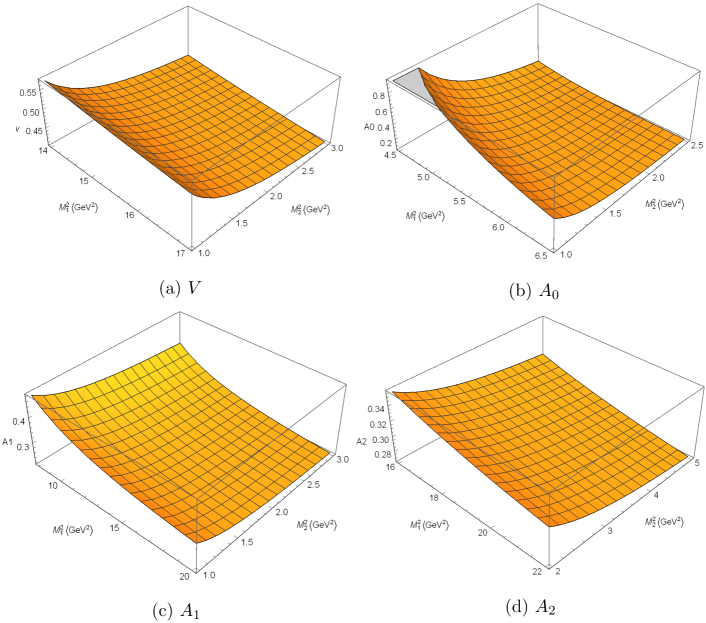
Figure 6: Form factors changing with $M_{1}^{2}$ and $M_{2}^{2}$.

Table 1: Requirements to select Borel Parameters $M_{1}^{2}$ and $M_{2}^{2}$ for each form factors $V(0)$, $A_{0}(0)$, $A_{1}(0)$ and $A_{2}(0)$

Form Factors	contribution	continuum of	continuum of
	of condensate	$B_{s}$ channel	$\phi$ channel
$V(0)$	$\leq 56.7\%$	$\leq 11\%$	$\leq 56\%$
$A_{0}(0)$	$\leq 14\%$	$\leq 10\%$	$\leq 50\%$
$A_{1}(0)$	$\leq 56\%$	$\leq 17.5\%$	$\leq 50\%$
$A_{2}(0)$	$\leq 5.2\%$	$\leq 17.2\%$	$\leq 54\%$

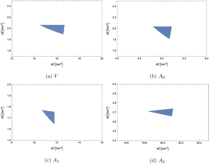
Figure 7: Selected regions of $M_{1}^{2}$ and $M_{2}^{2}$.

The final results for the form factors at $q^{2}=0$ are

$$V(0) = 0.45\pm 0.10,~{}~{}~{}~{}~{}~{}~{}~{}A_{0}(0)~{}=~{}0.30\pm 0.25,$$

$$A_{1}(0) = 0.32\pm 0.07,~{}~{}~{}~{}~{}~{}~{}A_{2}(0)~{}=~{}0.30\pm 0.07.$$ (28)

The uncertainties are obtained by varying the input parameters and Borel parameters in the stability regions.

We compare our results with other nonperturbative approaches such as LCSR R11 and CQM R12 in Table 2. The form factors for semileptonic decays of $B^{0}_{s}$ to $\phi$ meson have also been calculated by QCD sum rule in Ref. R15 . We do not list the value of $A^{\star}_{2}(0)=-0.44$ of Ref. R15 in Table 2, because the form factor $A^{\star}_{2}(0)$ defined in R15 does not directly correspond to the defination in our work. The relations of the form factors defined in Ref.R15 and ours are

$$V^{\star}(q^{2})=(-i)V(q^{2}),~{}~{}{A^{\star}_{0}}(q^{2})=(-i){A_{1}}(q^{2}),~{}~{}{A^{\star}_{1}}(q^{2})=(-i){A_{2}}(q^{2}),$$

$${A^{\star}_{2}}(q^{2})=\frac{(-i)(m_{B_{s}}+m_{\phi})}{q^{2}}\left[(m_{B_{s}}-m_{\phi})A_{2}(q^{2})-(m_{B_{s}}+m_{\phi})A_{1}(q^{2})+2m_{\phi}A_{1}(q^{2})\right],$$ (29)

where $V^{\star}(q^{2})$, ${A^{\star}_{0}}(q^{2})$, ${A^{\star}_{1}}(q^{2})$ and ${A^{\star}_{2}}(q^{2})$ denote the form factors defined in R15 .

Table 2: Comparison of our results of form factors with other work

	$A_{0}(0)$	$A_{1}(0)$	$A_{2}(0)$	$V(0)$
LCSR	$0.474$	$0.311$	$0.234$	$0.434$
CQM	$0.42$	$0.34$	$0.31$	$0.44$
SR	$A^{\star}_{2}(0)$	$-0.34$	$0.35$	$-0.47$
This work	$0.30\pm 0.25$	$0.32\pm 0.07$	$0.30\pm 0.07$	$0.45\pm 0.10$

Table 2 shows that our results for $A_{1}$, $A_{2}$ and $V$ are more consistent with the results of LCSR in Ref. R11 and CQM in Ref. R12 . Only $A_{0}$ is slightly smaller than theirs. The difference between the results of the form factors in Ref. R15 and ours is large. The reason is checked, that is: for the contribution of the condensate of the operator of dimension 3, the leading contribution is at the order of $(m_{s}/M_{i})^{0}$ in our calculation, which comes from the first term $\frac{1}{12}\delta_{\beta\alpha}$ of Eq. (20). But there are no such terms in the result of Ref. R15 , only terms like $(m_{b}m_{s}/M_{i}^{2})^{n}$ or $(m_{s}^{2}/M_{i}^{2})^{n}$ with $n\geq 1$ exist. The contributions of the operators of dimension 5 are also different.

In the next section we can see that the branching ratios of $B_{s}\to J\psi\phi$ calculated with the form factors obtained in this work are consistent with experimental data.

For the $q^{2}$-dependence of the form factors, we varied the value of $q^{2}$ by keeping it slightly larger than 0. We find that the $q^{2}$-dependence of $V(q^{2})$, $A_{0}(q^{2})$ and $A_{2}(q^{2})$ are well compatible with the pole-model R1 , which can be expressed as

$$V(q^{2})~{}= \frac{V(0)}{1-q^{2}/(m_{pole}^{V})^{2}},$$

$$A_{0}(q^{2})~{}= \frac{A_{0}(0)}{1-q^{2}/(m_{pole}^{A_{0}})^{2}},$$

$$A_{2}(q^{2})~{}= \frac{A_{2}(0)}{1-q^{2}/(m_{pole}^{A_{2}})^{2}},$$ (30)

while the $q^{2}$ dependence of $A_{1}(q^{2})$ is very weak.

We fit $V(q^{2})$, $A_{0}(q^{2})$ and $A_{2}(q^{2})$ with the pole model to our numerical results calculated from QCD sum rule. Then the relevant fitted pole masses are

$$m^{V}_{pole}~{}= 5.59\pm 0.27~{}\mbox{GeV},$$

$$m^{A_{0}}_{pole}~{}= 5.62\pm 2.38~{}\mbox{GeV},$$

$$m^{A_{2}}_{pole}~{}= 9.20\pm 0.40~{}\mbox{GeV}.$$ (31)

The fitted pole mass $m^{A_{2}}_{pole}$ is apparently larger than the other two pole masses, which means that the dependence of $A_{2}(q^{2})$ on $q^{2}$ is also weak, and it is almost as weak as $A_{1}(q^{2})$. This result implies that the dependence of the form factors on $q^{2}$ can not always be described by a real physical resonance pole that is associated with the transition current, because the mass of such resonance is usually far beyond the physical region of $q^{2}$ in the realistic decay process.

IV The Application of the Form Factors to the Branching Ratios

We use the form factors obtained in this work to calculate the time-dependent decay width and branching ratio of $\bar{B}^{0}_{s}\to J\psi\phi$ mode. For simplicity in checking whether the form factors obtained in this work can give predictions consistent with experiment, we only calculate the branching ratio in naive factorization approach here. The Feynman diagrams for $\bar{B}_{s}^{0}\to J/\psi\phi$ decay are shown in Fig.8.

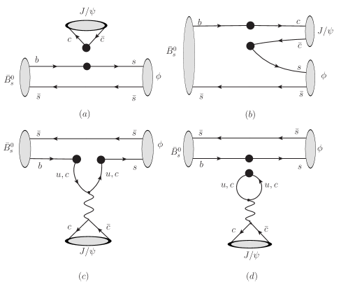
Figure 8: The Feynman diagrams for the decay of $\bar{B}_{s}^{0}\to J/\psi\phi$, “$\bullet$” denotes the effective vertex for the operator insertion.

The effective amplitude of $\bar{B}_{s}^{0}\to J/\psi\phi$ is

$$\mathcal{\bar{A}}_{eff}=\langle J/\psi\phi|\mathcal{H}_{eff}|\bar{B}_{s}^{0}\rangle,$$ (32)

where the effective Hamiltonian is

$$\mathcal{H}_{eff}=\frac{G_{F}}{\sqrt{2}}\left[V_{cb}V_{cs}^{*}(C_{1}O_{1}+C_{2}O_{2})-V_{tb}V_{ts}^{*}(\sum_{j=3}^{10}{C_{j}O_{j}})\right],$$

with

$$O_{1}=(\bar{c}_{i}b_{j})_{V-A}(\bar{s}_{j}c_{i})_{V-A},~{}~{}O_{2}=(\bar{c}_{i}b_{i})_{V-A}(\bar{s}_{j}c_{j})_{V-A},$$

$$O_{3}=(\bar{s}_{i}b_{i})_{V-A}(\bar{c}_{j}c_{j})_{V-A},~{}~{}O_{4}=(\bar{s}_{i}b_{j})_{V-A}(\bar{c}_{j}c_{i})_{V-A},$$

$$O_{5}=(\bar{s}_{i}b_{i})_{V-A}(\bar{c}_{j}c_{j})_{V+A},~{}~{}O_{6}=(\bar{s}_{i}b_{j})_{V-A}(\bar{c}_{j}c_{i})_{V+A},$$

$$O_{7}=\frac{3}{2}(\bar{s}_{i}b_{i})_{V-A}\frac{2}{3}(\bar{c}_{j}c_{j})_{V+A},~{}~{}O_{8}=\frac{3}{2}(\bar{s}_{i}b_{j})_{V-A}\frac{2}{3}(\bar{c}_{j}c_{i})_{V+A},$$

$$O_{9}=\frac{3}{2}(\bar{s}_{i}b_{i})_{V-A}\frac{2}{3}(\bar{c}_{j}c_{j})_{V-A},~{}~{}O_{10}=\frac{3}{2}(\bar{s}_{i}b_{j})_{V-A}\frac{2}{3}(\bar{c}_{j}c_{i})_{V-A}.$$

For Wilson coefficient $C_{i}(\mu)$, we take the value calculated by naive dimensional regularization(NDR) scheme up to the next-to-leading-order at renormalization scale $\mu=m_{b}$ as R10

$$C_{1}=-0.176;~{}C_{2}=1.078;~{}C_{3}=0.014;$$

$$C_{4}=-0.034;~{}C_{5}=0.008;~{}C_{6}=-0.039;$$

$$C_{7}=-0.011\alpha;~{}C_{8}=0.055\alpha;~{}C_{9}=-1.341\alpha;~{}C_{10}=0.264\alpha$$

where $\alpha$ is the electromagnetic coupling constant, which takes $\alpha=7.297\times 10^{-3}$.

We can divide the total effective amplitude into three parts

$$\mathcal{\bar{A}}_{eff}=\mathcal{\bar{A}}_{1}+\mathcal{\bar{A}}_{2}+\mathcal{\bar{A}}_{3},$$ (33)

where $\mathcal{\bar{A}}_{1}$ denotes the contribution of the two tree diagrams of Fig.8 (a) and (b), $\mathcal{\bar{A}}_{2}$ the contribution of Fig.8 (c), and $\mathcal{\bar{A}}_{3}$ the contribution of Fig.8 (d).

The amplitude of the two tree diagrams is

$$\begin{split}\mathcal{\bar{A}}_{1}=&\frac{G_{F}}{\sqrt{2}}\left[V_{cb}V_{cs}^{*}(C_{1}+\frac{C_{2}}{N_{c}})-V_{tb}V_{ts}^{*}(C_{3}+\frac{C_{4}}{N_{c}}+C_{5}+\frac{C_{6}}{N_{c}}+C_{7}+\frac{C_{8}}{N_{c}}+C_{9}+\frac{C_{10}}{N_{c}})\right]\\ &\langle J/\psi|\bar{c}\gamma^{\nu}(1-\gamma_{5})c|0\rangle\langle\phi|\bar{s}\gamma_{\nu}(1-\gamma_{5})b|\bar{B}_{s}^{0}\rangle,\end{split}$$ (34)

while the amplitudes of the two penguin diagrams are

$$\begin{split}\mathcal{\bar{A}}_{2}=&\frac{G_{F}}{\sqrt{2}}C_{1}\left[V_{ub}V_{us}^{*}\frac{Q_{u}^{2}\alpha}{\pi}\int_{0}^{1}{2\bar{x}x(1+\ln{\frac{a^{2}}{\mu^{2}}})}dx+V_{cb}V_{cs}^{*}\frac{Q_{c}^{2}\alpha}{\pi}\int_{0}^{1}{2\bar{x}x(1+\ln{\frac{b^{2}}{\mu^{2}}})}dx\right]\\ &\langle J/\psi|\bar{c}\gamma^{\nu}(1-\gamma_{5})c|0\rangle\langle\phi|\bar{s}\gamma_{\nu}(1-\gamma_{5})b|\bar{B}_{s}^{0}\rangle,\end{split}$$ (35)

and

$$\begin{split}\mathcal{\bar{A}}_{3}=&\frac{G_{F}}{\sqrt{2}}C_{1}\left[V_{ub}V_{us}^{*}\frac{Q_{u}^{2}\alpha}{\pi}\int_{0}^{1}{2\bar{x}x\ln{\frac{a^{2}}{\mu^{2}}}}dx+V_{cb}V_{cs}^{*}\frac{Q_{c}^{2}\alpha}{\pi}\int_{0}^{1}{2\bar{x}x\ln{\frac{b^{2}}{\mu^{2}}}}dx\right]\\ &\langle J/\psi|\bar{c}\gamma^{\nu}(1-\gamma_{5})c|0\rangle\langle\phi|\bar{s}\gamma_{\nu}(1-\gamma_{5})b|\bar{B}_{s}^{0}\rangle.\end{split}$$ (36)

Because of $\bar{B}_{s}^{0}-B_{s}^{0}$ mixing, we should consider the decay amplitude of $B_{s}^{0}\to J/\psi\phi$ in the analysis of time-dependent decays. Similarly we denote $\mathcal{A}_{eff}=\langle J/\psi\phi|\mathcal{H}_{eff}|B_{s}^{0}\rangle$ and

$$\mathcal{A}_{eff}=\mathcal{A}_{1}+\mathcal{A}_{2}+\mathcal{A}_{3},$$ (37)

with

$$\begin{split}\mathcal{A}_{1}=&\frac{G_{F}}{\sqrt{2}}\left[V_{cb}^{*}V_{cs}(C_{1}+\frac{C_{2}}{N_{c}})-V_{tb}^{*}V_{ts}(C_{3}+\frac{C_{4}}{N_{c}}+C_{5}+\frac{C_{6}}{N_{c}}+C_{7}+\frac{C_{8}}{N_{c}}+C_{9}+\frac{C_{10}}{N_{c}})\right]\\ &\langle J/\psi|\bar{c}\gamma^{\nu}(1-\gamma_{5})c|0\rangle\langle\phi|\bar{b}\gamma_{\nu}(1-\gamma_{5})s|B_{s}^{0}\rangle,\end{split}$$ (38)

$$\begin{split}\mathcal{A}_{2}=&\frac{G_{F}}{\sqrt{2}}C_{1}\left[V_{ub}^{*}V_{us}\frac{Q_{u}^{2}\alpha}{\pi}\int_{0}^{1}{2\bar{x}x(1+\ln{\frac{a^{2}}{\mu^{2}}})}dx+V_{cb}^{*}V_{cs}\frac{Q_{c}^{2}\alpha}{\pi}\int_{0}^{1}{2\bar{x}x(1+\ln{\frac{b^{2}}{\mu^{2}}})}dx\right]\\ &\langle J/\psi|\bar{c}\gamma^{\nu}(1-\gamma_{5})c|0\rangle\langle\phi|\bar{b}\gamma_{\nu}(1-\gamma_{5})s|B_{s}^{0}\rangle,\end{split}$$ (39)

$$\begin{split}\mathcal{A}_{3}=&\frac{G_{F}}{\sqrt{2}}C_{1}\left[V_{ub}^{*}V_{us}\frac{Q_{u}^{2}\alpha}{\pi}\int_{0}^{1}{2\bar{x}x\ln{\frac{a^{2}}{\mu^{2}}}}dx+V_{cb}^{*}V_{cs}\frac{Q_{c}^{2}\alpha}{\pi}\int_{0}^{1}{2\bar{x}x\ln{\frac{b^{2}}{\mu^{2}}}}dx\right]\\ &\langle J/\psi|\bar{c}\gamma^{\nu}(1-\gamma_{5})c|0\rangle\langle\phi|\bar{b}\gamma_{\nu}(1-\gamma_{5})s|B_{s}^{0}\rangle,\end{split}$$ (40)

where $\bar{x}=1-x$, $a^{2}=m_{u}^{2}-x(1-x)q^{2}$, $b^{2}=m_{c}^{2}-x(1-x)q^{2}$, and $q$ is the transition momentum. $G_{F}$ is the Fermi constant, $N_{c}=3$ the color quantum number of quarks, $Q_{q}(q=u,c)$ the charge of relevant quarks, $C_{i}(i=1,2,...,10.)$ the Wilson coefficients, and $V_{qb},V_{qs}\;(q=u,c,t)$ the relevant CKM matrix elements, respectively.

There are three polarization states for $\phi$ meson: one longitudinal state and two transverse polarization states (right-handed and left-handed). We define

$$h_{\lambda}~{}\equiv\langle J/\psi|\bar{c}\gamma^{\nu}(1-\gamma_{5})c|0\rangle\langle\phi|\bar{s}\gamma_{\nu}(1-\gamma_{5})b|\bar{B}_{s}^{0}\rangle,$$ (41)

then using Eq. (II) and the following matrix elements for $J/\psi$ meson

$$\langle 0|\bar{c}\gamma_{\mu}c|{J/\psi}\rangle=m_{J/\psi}f_{J/\psi}\varepsilon_{\mu}^{(\lambda)},$$

$$\langle 0|\bar{c}\gamma_{\mu}\gamma_{5}c|J/\psi\rangle=0,$$ (42)

we can obtain, for the longitudinal polarization states of the vector mesons

$$h_{0}~{}=\frac{if_{J/\psi}}{2m_{\phi}}\left[(m_{B_{s}}^{2}-m_{\phi}^{2}-{m_{J/\psi}}^{2})(m_{B_{s}}+m_{\phi})A_{1}(q^{2})-\frac{4{m_{B_{s}}}^{2}{p_{\phi}}^{2}}{m_{B_{s}}+m_{\phi}}A_{2}(q^{2})\right],$$ (43)

and for the transverse polarization states

$$h_{\pm}~{}=i{f_{J/\psi}}{m_{J/\psi}}\left[(m_{B_{s}}+m_{\phi})A_{1}(q^{2})\mp\frac{2m_{B_{s}}p_{\phi}V(q^{2})}{m_{B_{s}}+m_{\phi}}\right].$$ (44)

where ${p_{\phi}}=\frac{1}{2m_{B_{s}}}\sqrt{\left[m_{B_{s}}^{2}-(m_{\phi}+m_{J/\psi}^{2})\right]\left[m_{B_{s}}^{2}-(m_{\phi}-m_{J/\psi}^{2})\right]}$ is the momentum of $\phi$ meson in the rest frame of $B_{s}$.

We can write $|\mathcal{\bar{A}}_{eff}|^{2}$ in terms of the sum of one longitudinal and two transverse polarization amplitudes squared

$$|\mathcal{\bar{A}}_{eff}|^{2}=|(\mathcal{\bar{A}}_{eff})_{L}|^{2}+|(\mathcal{\bar{A}}_{eff})_{+}|^{2}+|(\mathcal{\bar{A}}_{eff})_{-}|^{2},$$ (45)

where

$$\begin{split}|(\mathcal{\bar{A}}_{eff})_{L}|^{2}=|(\mathcal{\bar{A}}_{1})_{L}|^{2}+|(\mathcal{\bar{A}}_{2})_{L}|^{2}+|(\mathcal{\bar{A}}_{3})_{L}|^{2},\\ |(\mathcal{\bar{A}}_{eff})_{\pm}|^{2}=|(\mathcal{\bar{A}}_{1})_{\pm}|^{2}+|(\mathcal{\bar{A}}_{2})_{\pm}|^{2}+|(\mathcal{\bar{A}}_{3})_{\pm}|^{2}.\end{split}$$ (46)

In the same way, $|\mathcal{A}_{eff}|^{2}$ can be written as

$$|\mathcal{A}_{eff}|^{2}=|(\mathcal{A}_{eff})_{L}|^{2}+|(\mathcal{A}_{eff})_{+}|^{2}+|(\mathcal{A}_{eff})_{-}|^{2},$$ (47)

where

$$\begin{split}|(\mathcal{A}_{eff})_{L}|^{2}=|(\mathcal{A}_{1})_{L}|^{2}+|(\mathcal{A}_{2})_{L}|^{2}+|(\mathcal{A}_{3})_{L}|^{2},\\ |(\mathcal{A}_{eff})_{\pm}|^{2}=|(\mathcal{A}_{1})_{\pm}|^{2}+|(\mathcal{A}_{2})_{\pm}|^{2}+|(\mathcal{A}_{3})_{\pm}|^{2}.\end{split}$$ (48)

The relevant expressions for the terms in the right hand of Eqs.(46) and (48) are given in the Appendix C. Then we obtain the transverse time-dependent decay width

$$\begin{split}\Gamma(\bar{B}_{s}^{0}(t)\to J/\psi\phi)_{T}^{\pm}~{}=&\frac{p_{\phi}}{8\pi m_{B_{s}}^{2}}\frac{1}{2}e^{-\Gamma_{B_{s}}t}\left[(|(\mathcal{A}_{eff})_{\pm}|^{2}+|(\mathcal{\bar{A}}_{eff})_{\pm}|^{2})\cosh{\frac{\Delta\Gamma}{2}t}\right.\\ &\left.-(|(\mathcal{A}_{eff})_{\pm}|^{2}-|(\mathcal{\bar{A}}_{eff})_{\pm}|^{2})\cos{{\Delta m}t}\right.\\ &\left.+2Re(\frac{p}{q}(\mathcal{A}_{eff})_{\pm}({\mathcal{\bar{A}}_{eff}}^{*})_{\pm})\sinh{\frac{\Delta\Gamma}{2}t}-2Im(\frac{p}{q}(\mathcal{A}_{eff})_{\pm}({\mathcal{\bar{A}}_{eff}}^{*})_{\pm})\sin{{\Delta m}t}\right],\end{split}$$ (49)

and the longitudinal time-dependent decay width

$$\begin{split}\Gamma(\bar{B}_{s}^{0}(t)\to J/\psi\phi)_{L}~{}=&\frac{p_{\phi}}{8\pi m_{B_{s}}^{2}}\frac{1}{2}e^{-\Gamma_{B_{s}}t}\left[(|(\mathcal{A}_{eff})_{L}|^{2}+|(\mathcal{\bar{A}}_{eff})_{L}|^{2})\cosh{\frac{\Delta\Gamma}{2}t}\right.\\ &\left.-(|(\mathcal{A}_{eff})_{L}|^{2}-|(\mathcal{\bar{A}}_{eff})_{L}|^{2})\cos{{\Delta m}t}\right.\\ &\left.+2Re(\frac{p}{q}(\mathcal{A}_{eff})_{L}({\mathcal{\bar{A}}_{eff}}^{*})_{L})\sinh{\frac{\Delta\Gamma}{2}t}-2Im(\frac{p}{q}(\mathcal{A}_{eff})_{L}({\mathcal{\bar{A}}_{eff}}^{*})_{L})\sin{{\Delta m}t}\right].\end{split}$$ (50)

We take $\frac{p}{q}=\frac{V_{tb}V_{ts}^{*}}{V_{tb}^{*}V_{ts}}=e^{-i2\beta_{s}}$, $\beta_{s}=0.0185$, $\frac{\Delta\Gamma}{\Gamma_{B_{s}}}=0.122$, $\frac{\Delta m}{\Gamma_{B_{s}}}=26.79$ and the total decay width of $B_{s}$ meson is $\Gamma_{B_{s}}=4.362\times 10^{-13}\;\mbox{GeV}$ R17 . Finally, the combined transverse and total time-dependent decay widths are

$$\begin{split}\Gamma(\bar{B}_{s}^{0}(t)\to J/\psi\phi)_{T}=\Gamma(\bar{B}_{s}^{0}(t)\to J/\psi\phi)_{T}^{+}+\Gamma(\bar{B}_{s}^{0}(t)\to J/\psi\phi)_{T}^{-},\\ \Gamma(\bar{B}_{s}^{0}(t)\to J/\psi\phi)=\Gamma(\bar{B}_{s}^{0}(t)\to J/\psi\phi)_{L}+\Gamma(\bar{B}_{s}^{0}(t)\to J/\psi\phi)_{T}.\end{split}$$ (51)

And the total time-dependent decay width is R17

$$\begin{split}\Gamma(\bar{B}_{s}^{0}(t)\to J/\psi\phi)~{}=&\frac{p_{\phi}}{8\pi m_{B_{s}}^{2}}\frac{1}{2}e^{-\Gamma_{B_{s}}t}\left[(|\mathcal{A}_{eff}|^{2}+|\mathcal{\bar{A}}_{eff}|^{2})\cosh{\frac{\Delta\Gamma}{2}t}\right.\\ &\left.-(|\mathcal{A}_{eff}|^{2}-|\mathcal{\bar{A}}_{eff}|^{2})\cos{{\Delta m}t}+2Re(\frac{p}{q}\mathcal{A}_{eff}{\mathcal{\bar{A}}_{eff}}^{*})\sinh{\frac{\Delta\Gamma}{2}t}\right.\\ &\left.-2Im(\frac{p}{q}\mathcal{A}_{eff}{\mathcal{\bar{A}}_{eff}}^{*})\sin{{\Delta m}t}\right].\end{split}$$ (52)

Similarly, we can also obtain the total time-dependent decay width of $B_{s}^{0}(t)\to J/\psi\phi$, which is R17

$$\begin{split}\Gamma(B_{s}^{0}(t)\to J/\psi\phi)~{}=&\frac{p_{\phi}}{8\pi m_{B_{s}}^{2}}\frac{1}{2}e^{-\Gamma_{B_{s}}t}\left[(|\mathcal{A}_{eff}|^{2}+|\mathcal{\bar{A}}_{eff}|^{2})\cosh{\frac{\Delta\Gamma}{2}t}\right.\\ &\left.+(|\mathcal{A}_{eff}|^{2}-|\mathcal{\bar{A}}_{eff}|^{2})\cos{{\Delta m}t}+2Re(\frac{q}{p}{\mathcal{A}_{eff}}^{*}\mathcal{\bar{A}}_{eff})\sinh{\frac{\Delta\Gamma}{2}t}\right.\\ &\left.-2Im(\frac{q}{p}{\mathcal{A}_{eff}}^{*}\mathcal{\bar{A}}_{eff})\sin{{\Delta m}t}\right].\end{split}$$ (53)

Integrating the above time-dependent decay widths over $t$ from zero to infinity, we can get the relevant branching ratios Duni2001 ; Bruyn2012

$$\begin{split}Br(B_{s}\to J/\psi\phi)_{T}=\frac{1}{2}\int_{0}^{\infty}\left[{\Gamma(\bar{B}_{s}^{0}(t)\to J/\psi\phi)_{T}}+\Gamma(B_{s}^{0}(t)\to J/\psi\phi)_{T}\right]dt,\\ Br(B_{s}\to J/\psi\phi)_{L}=\frac{1}{2}\int_{0}^{\infty}\left[{\Gamma(\bar{B}_{s}^{0}(t)\to J/\psi\phi)_{L}}+\Gamma(B_{s}^{0}(t)\to J/\psi\phi)_{L}\right]dt,\\ Br(B_{s}\to J/\psi\phi)_{total}=\frac{1}{2}\int_{0}^{\infty}\left[{\Gamma(\bar{B}_{s}^{0}(t)\to J/\psi\phi)}+\Gamma(B_{s}^{0}(t)\to J/\psi\phi)\right]dt.\end{split}$$ (54)

Substituting the values for the relevant parameters and quantities into the above equation we can get

$$\begin{split}Br(B_{s}\to J/\psi\phi)_{L}=(0.42\pm 0.17)\times 10^{-3},\\ Br(B_{s}\to J/\psi\phi)_{T}=(0.50\pm 0.09)\times 10^{-3},\end{split}$$ (55)

and the total total decay branching ratio is

$$Br(B_{s}\to J/\psi\phi)=(0.92\pm 0.26)\times 10^{-3},$$ (56)

which are in good agreement with experimental data within uncertainties R17 :

$$Br(B_{s}\to J/\psi\phi)_{L}^{exp}=(0.56\pm 0.04)\times 10^{-3},$$

$$Br(B_{s}\to J/\psi\phi)_{T}^{exp}=(0.52\pm 0.04)\times 10^{-3},$$

$$Br(B_{s}\to J/\psi\phi)^{exp}=(1.08\pm 0.08)\times 10^{-3}.$$

V Summary

We calculate the $\bar{B}^{0}_{s}\to\phi$ transition form factors by QCD sum rule method. The form factors are expressed in terms of two Borel parameters $M_{1}^{2}$, $M_{2}^{2}$ and relevant Borel transformation coefficients. We take the two Borel parameters $M_{1}^{2}$, $M_{2}^{2}$ as independent parameters and find the “stable windows” in the two-dimensional area of $M_{1}^{2}$ and $M_{2}^{2}$ for the transition form factors $V$, $A_{0}$, $A_{1}$ and $A_{2}$. Our results are compatible with that obtained by LCSR and CQM methods in the literature. Finally, we apply the results of the transition form factors $V$, $A_{0}$, $A_{1}$ and $A_{2}$ to the nonleptonic decay process of $\bar{B}_{s}^{0}\to J/\psi\phi$. We calculate the branching ratios for all the possible polarization states of the vector mesons. The branching ratios we obtained are well consistent with experimental data.

$$\begin{array}[]{ll}I=\int d^{4}k\delta(k^{2}-m_{0}^{2})\delta[(k+p_{1})^{2}-m_{1}^{2}]\delta[(k+p_{2})^{2}-m_{2}^{2}]=\frac{\pi}{2\sqrt{\lambda}},\end{array}$$

$$\begin{array}[]{ll}I_{\mu}=\int d^{4}kk_{\mu}\delta(k^{2}-m_{0}^{2})\delta[(k+p_{1})^{2}-m_{1}^{2}]\delta\ [(k+p_{2})^{2}-m_{2}^{2}]\\ \equiv a_{1}p_{1\mu}+b_{1}p_{2\mu},\\[11.38109pt] \left\{\begin{array}[]{ll}a_{1}~{}=&-\frac{\pi}{2\lambda^{3/2}}[s_{2}(-s_{1}+s_{2}-q^{2})+(s_{1}+s_{2}-q^{2})(m_{0}^{2}-m_{2}^{2})\\[8.53581pt] &~{}-2s_{2}(m_{0}^{2}-m_{1}^{2})],\\[8.53581pt] b_{1}~{}=&-\frac{\pi}{2\lambda^{3/2}}[s_{1}(-s_{2}+s_{1}-q^{2})+(s_{1}+s_{2}-q^{2})(m_{0}^{2}-m_{1}^{2})\\[8.53581pt] &~{}-2s_{1}(m_{0}^{2}-m_{2}^{2})],\end{array}\right.\end{array}$$

$$\begin{array}[]{ll}I_{\mu\nu}=\int d^{4}kk_{\mu}k_{\nu}\delta(k^{2}-m_{0}^{2})\delta[(k+p_{1})^{2}-m_{1}^{2}]\delta\ [(k+p_{2})^{2}-m_{2}^{2}]\\ \equiv a_{2}p_{1\mu}p_{1\nu}+b_{2}p_{2\mu\nu}+c_{2}(p_{1\mu}p_{2\nu}+p_{1\nu}p_{2\mu})+d_{2}g_{\mu\nu},\\[11.38109pt] \left\{\begin{array}[]{ll}D_{1}~{}\equiv&s_{1}-m_{1}^{2}+m_{0}^{2},~{}~{}~{}~{}~{}D_{2}\equiv s_{2}-m_{2}^{2}+m_{0}^{2},\\[8.53581pt] a_{2}~{}=&\frac{\pi}{\lambda^{3/2}}m_{0}^{2}s_{2}+\frac{1}{\lambda}[3s_{2}D_{1}a_{1}-(s_{1}+s_{2}-q^{2})D_{2}b_{1}+s_{2}D_{2}b_{1}],\\[8.53581pt] b_{2}~{}=&\frac{\pi}{\lambda^{3/2}}m_{0}^{2}s_{1}+\frac{1}{\lambda}[s_{1}D_{1}a_{1}-(s_{1}+s_{2}-q^{2})D_{1}b_{1}+3s_{1}D_{2}b_{1}],\\[8.53581pt] c_{2}~{}=&-\frac{\pi}{\lambda^{3/2}}m_{0}^{2}\frac{1}{2}(s_{1}+s_{2}-q^{2})\\[8.53581pt] &-\frac{1}{\lambda}[\frac{1}{2}(s_{1}+s_{2}-q^{2})D_{1}a_{1}-2s_{2}D_{1}b_{1}+\frac{3}{2}(s_{1}+s_{2}-q^{2})D_{2}b_{1}],\\[8.53581pt] d_{2}~{}=&\frac{\pi}{4\sqrt{\lambda}}+\frac{1}{4}[D_{1}a_{1}+D_{2}b_{1}].\end{array}\right.\end{array}$$

where $\lambda(s_{1},s_{2},q^{2})=(s_{1}+s_{2}-q^{2})^{2}-4s_{1}s_{2}$.

Appendix B

The results of relevant Borel transformed Coefficients for the transition form factors in Eq. (13) are given here.

1) Borel transformed $f_{0}$:

$$\hat{B}f_{0}=\hat{B}f_{0}^{pert}+\hat{B}f_{0}^{(3)}+\hat{B}f_{0}^{(5)}+\hat{B}f_{0}^{(6)}\;,$$

where,

$$\begin{array}[]{ll}\hat{B}f_{0}^{pert}~{}=&\int^{s_{2}^{0}}_{4m_{s}^{2}}ds_{2}\int^{s_{1}^{0}}_{s_{1}^{L}}ds_{1}\displaystyle\frac{3e^{-s_{1}/M_{1}^{2}-s_{2}/M_{2}^{2}}}{4M_{1}^{2}M_{2}^{2}\pi^{2}\lambda^{3/2}}[-{s_{2}}m_{b}(2m_{s}^{2}+q^{2}\\ &+{s_{1}}-{s_{2}})-2{s_{2}}m_{b}^{2}m_{s}+2{s_{2}}m_{b}^{3}+m_{s}(\lambda+2{s_{2}}m_{s}^{2}\\ &+q^{2}{s_{2}}+{s_{1}}{s_{2}}-{s_{2}}^{2})],\end{array}$$

where $\lambda=(s_{1}+s_{2}-q^{2})^{2}-4s_{1}s_{2}$. The lower limit of the integration $s_{1}^{L}$ is determined by requiring that all internal quarks are on their mass shell R1

$$s_{1}^{L}=\frac{m_{b}^{2}}{m_{b}^{2}-q^{2}}s_{2}+m_{b}^{2}\;,$$

and

$$\begin{array}[]{ll}\hat{B}f_{0}^{(3)}~{}=&-\displaystyle\frac{e^{-m_{b}^{2}/M_{1}^{2}-m_{s}^{2}/M_{2}^{2}}}{6M_{1}^{8}M_{2}^{8}}[{M_{1}}^{2}{M_{2}}^{2}m_{b}^{2}m_{s}^{2}({M_{1}}^{2}+{M_{2}}^{2})(3{M_{2}}^{2}-m_{s}^{2})\\ &+{M_{1}}^{2}{M_{2}}^{2}m_{b}m_{s}({M_{2}}^{2}m_{s}^{2}({M_{1}}^{2}+{M_{2}}^{2}+q^{2})-m_{s}^{4}({M_{1}}^{2}+{M_{2}}^{2})\\ &-3{M_{1}}^{2}{M_{2}}^{4})-{M_{2}}^{4}m_{b}^{3}m_{s}^{3}({M_{1}}^{2}+{M_{2}}^{2})+{M_{1}}^{4}(-3{M_{2}}^{4}m_{s}^{2}({M_{1}}^{2}\\ &+q^{2})+{M_{2}}^{2}m_{s}^{4}(4{M_{1}}^{2}+4{M_{2}}^{2}+q^{2})-m_{s}^{6}({M_{1}}^{2}+{M_{2}}^{2})\\ &+6{M_{1}}^{2}{M_{2}}^{6})]\times\langle\bar{s}s\rangle\;,\end{array}$$

$$\begin{array}[]{ll}\hat{B}f_{0}^{(5)}~{}=&-\displaystyle\frac{e^{-m_{b}^{2}/M_{1}^{2}-m_{s}^{2}/M_{2}^{2}}}{12M_{1}^{8}M_{2}^{8}}[{M_{1}}^{2}{M_{2}}^{2}m_{b}m_{s}(m_{s}^{2}({M_{1}}^{2}+{M_{2}}^{2})\\ &+{M_{2}}^{2}(-2{M_{1}}^{2}+2{M_{2}}^{2}-q^{2}))-{M_{1}}^{2}{M_{2}}^{2}m_{b}^{2}({M_{1}}^{2}\\ &+{M_{2}}^{2})(3{M_{2}}^{2}-m_{s}^{2})+{M_{2}}^{4}m_{b}^{3}m_{s}({M_{1}}^{2}+{M_{2}}^{2})\\ &+{M_{1}}^{4}(-{M_{2}}^{2}m_{s}^{2}(5{M_{1}}^{2}+3{M_{2}}^{2}+q^{2})+m_{s}^{4}({M_{1}}^{2}+{M_{2}}^{2})\\ &+{M_{2}}^{4}(3({M_{2}}^{2}+q^{2})-{M_{1}}^{2}))]\times g\langle\bar{s}\sigma TGs\rangle\;,\end{array}$$

$$\begin{array}[]{ll}\hat{B}f_{0}^{(6)}~{}=&\displaystyle\frac{e^{-m_{b}^{2}/M_{1}^{2}-m_{s}^{2}/M_{2}^{2}}}{81M_{1}^{8}M_{2}^{8}(m_{b}^{2}-q^{2})m_{s}^{3}}[{M_{1}}^{2}{M_{2}}^{2}m_{b}^{4}m_{s}^{4}({M_{1}}^{2}+{M_{2}}^{2})\\ &+{M_{2}}^{4}m_{b}^{5}m_{s}^{3}({M_{1}}^{2}+{M_{2}}^{2})+{M_{2}}^{2}m_{b}^{3}m_{s}^{3}({M_{1}}^{2}m_{s}^{2}({M_{1}}^{2}+{M_{2}}^{2})\\ &-{M_{2}}^{2}(-2{M_{1}}^{4}+{M_{1}}^{2}(13{M_{2}}^{2}+2q^{2})+{M_{2}}^{2}q^{2}))\\ &+{M_{1}}^{2}{M_{2}}^{2}m_{b}m_{s}(36{M_{1}}^{4}{M_{2}}^{4}(e^{\frac{m_{s}^{2}}{{M_{2}}^{2}}}-1)+{M_{2}}^{2}q^{2}m_{s}^{2}(-2{M_{1}}^{2}\\ &+13{M_{2}}^{2}+q^{2})-q^{2}m_{s}^{4}({M_{1}}^{2}+{M_{2}}^{2}))+m_{b}^{2}(54{M_{1}}^{6}{M_{2}}^{4}m_{s}^{2}\\ &-54{M_{1}}^{6}{M_{2}}^{6}(e^{\frac{m_{s}^{2}}{{M_{2}}^{2}}}-1)-{M_{1}}^{2}{M_{2}}^{2}m_{s}^{4}({M_{1}}^{4}+2{M_{1}}^{2}(5{M_{2}}^{2}+q^{2})\\ &+{M_{2}}^{2}q^{2}){M_{1}}^{4}m_{s}^{6}({M_{1}}^{2}+{M_{2}}^{2}))+{M_{1}}^{4}({M_{2}}^{2}q^{2}m_{s}^{4}({M_{1}}^{2}+10{M_{2}}^{2}\\ &+q^{2})-q^{2}m_{s}^{6}({M_{1}}^{2}+{M_{2}}^{2})+54{M_{1}}^{2}{M_{2}}^{6}q^{2}(e^{\frac{m_{s}^{2}}{{M_{2}}^{2}}}-1)\\ &-18{M_{1}}^{2}{M_{2}}^{4}m_{s}^{2}({M_{2}}^{2}(e^{\frac{m_{s}^{2}}{{M_{2}}^{2}}}-1)+3q^{2})]\times g^{2}\langle\bar{s}s\rangle^{2}\;.\end{array}$$

2) Borel transformed result for $f_{1}+f_{3}$ :

$$\hat{B}(f_{1}+f_{3})=\hat{B}f_{+}^{pert}+\hat{B}f_{+}^{(3)}+\hat{B}f_{+}^{(5)}+\hat{B}f_{+}^{(6)}\;,$$

where

$$\begin{array}[]{ll}\hat{B}f_{+}^{pert}~{}=&\int^{s_{2}^{0}}_{4m_{s}^{2}}ds_{2}\int^{s_{1}^{0}}_{s_{1}^{L}}ds_{1}\displaystyle\frac{3e^{-s_{1}/M_{1}^{2}-s_{2}/M_{2}^{2}}}{4M_{1}^{2}M_{2}^{2}\pi^{2}\lambda^{5/2}}\{2{s_{2}}m_{b}^{3}(2q^{2}(3m_{s}^{2}+{s_{1}}+{s_{2}})+2q^{4}\\ &+\lambda-6m_{s}^{2}({s_{1}}-{s_{2}})-4{s_{1}}^{2}+8{s_{1}}{s_{2}}-4{s_{2}}^{2})+2{s_{2}}m_{b}^{2}m_{s}(-2q^{2}(3m_{s}^{2}+{s_{1}}+{s_{2}})\\ &-2q^{4}-3\lambda+6m_{s}^{2}({s_{1}}-{s_{2}})+4{s_{1}}^{2}-8{s_{1}}{s_{2}}+4{s_{2}}^{2})+m_{b}(q^{2}(-2m_{s}^{2}(\lambda+2{s_{1}}{s_{2}}+2{s_{2}}^{2})\\ &-6{s_{2}}m_{s}^{4}+{s_{2}}(-\lambda+2{s_{1}}^{2}-6{s_{1}}{s_{2}}+4{s_{2}}^{2}))-2{s_{2}}q^{4}(2m_{s}^{2}+2{s_{1}}+{s_{2}})+2m_{s}^{2}(4{s_{1}}^{2}{s_{2}}\\ &+\lambda{s_{1}}-8{s_{1}}{s_{2}}^{2}+4{s_{2}}^{3}-2\lambda{s_{2}})+6{s_{2}}m_{s}^{4}({s_{1}}-{s_{2}})+{s_{2}}({s_{1}}-{s_{2}})(-\lambda+2{s_{1}}^{2}\\ &-4{s_{1}}{s_{2}}+2{s_{2}}^{2}))+6{s_{2}}m_{b}^{4}m_{s}(q^{2}-{s_{1}}+{s_{2}})-6{s_{2}}m_{b}^{5}(q^{2}-{s_{1}}+{s_{2}})\\ &+m_{s}(q^{2}(2m_{s}^{2}(\lambda+2{s_{1}}{s_{2}}+2{s_{2}}^{2})+6{s_{2}}m_{s}^{4}+{s_{2}}(3\lambda-2{s_{1}}^{2}+6{s_{1}}{s_{2}}-4{s_{2}}^{2}))\\ &+2{s_{2}}q^{4}(2m_{s}^{2}+2{s_{1}}+{s_{2}})+\lambda^{2}-2m_{s}^{2}(4{s_{1}}^{2}{s_{2}}+\lambda{s_{1}}-8{s_{1}}{s_{2}}^{2}+4{s_{2}}^{3}-4\lambda{s_{2}})\\ &+6{s_{2}}m_{s}^{4}({s_{2}}-{s_{1}})-2{s_{1}}^{3}{s_{2}}+6{s_{1}}^{2}{s_{2}}^{2}-6{s_{1}}{s_{2}}^{3}+3\lambda{s_{1}}{s_{2}}+2{s_{2}}^{4}-3\lambda{s_{2}}^{2})\}\;,\end{array}$$

$$\begin{array}[]{ll}\hat{B}f_{+}^{(3)}~{}=&-\displaystyle\frac{e^{-m_{b}^{2}/M_{1}^{2}-m_{s}^{2}/M_{2}^{2}}}{6M_{1}^{8}M_{2}^{8}}\{-{M_{1}}^{2}{M_{2}}^{2}m_{b}m_{s}({M_{2}}^{2}m_{s}^{2}(-q^{2}+{M_{1}}^{2}+{M_{2}}^{2})\\ &+m_{s}^{4}({M_{1}}^{2}+{M_{2}}^{2})+3{M_{1}}^{2}{M_{2}}^{4})+{M_{1}}^{4}({M_{2}}^{2}m_{s}^{4}(q^{2}+4({M_{1}}^{2}+{M_{2}}^{2}))\\ &-3{M_{2}}^{4}m_{s}^{2}(q^{2}+{M_{1}}^{2}-2{M_{2}}^{2})-m_{s}^{6}({M_{1}}^{2}+{M_{2}}^{2})+6{M_{1}}^{2}{M_{2}}^{6})\\ &+{M_{1}}^{2}{M_{2}}^{2}m_{b}^{2}m_{s}^{2}({M_{1}}^{2}+{M_{2}}^{2})(3{M_{2}}^{2}-m_{s}^{2})-{M_{2}}^{4}m_{b}^{3}m_{s}^{3}({M_{1}}^{2}\\ &+{M_{2}}^{2})\}\times\langle\bar{s}s\rangle\;,\end{array}$$

$$\begin{array}[]{ll}\hat{B}f_{+}^{(5)}~{}=&\displaystyle\frac{e^{-m_{b}^{2}/M_{1}^{2}-m_{s}^{2}/M_{2}^{2}}}{12M_{1}^{8}M_{2}^{8}}\{q^{2}({M_{1}}^{2}{M_{2}}^{4}m_{b}m_{s}+{M_{1}}^{4}{M_{2}}^{2}(m_{s}^{2}-3{M_{2}}^{2}))\\ &-{M_{1}}^{2}{M_{2}}^{2}m_{b}m_{s}(m_{s}^{2}({M_{1}}^{2}+{M_{2}}^{2})+2{M_{2}}^{2}({M_{1}}^{2}+2{M_{2}}^{2}))\\ &+{M_{1}}^{2}{M_{2}}^{2}m_{b}^{2}({M_{1}}^{2}+{M_{2}}^{2})(3{M_{2}}^{2}-m_{s}^{2})-{M_{2}}^{4}m_{b}^{3}m_{s}({M_{1}}^{2}+{M_{2}}^{2})\\ &+{M_{1}}^{4}(-m_{s}^{4}({M_{1}}^{2}+{M_{2}}^{2})+m_{s}^{2}(5{M_{1}}^{2}{M_{2}}^{2}+7{M_{2}}^{4})\\ &+{M_{2}}^{4}({M_{1}}^{2}+3{M_{2}}^{2}))\}\times g\langle\bar{s}\sigma TGs\rangle\;,\end{array}$$

$$\begin{array}[]{ll}\hat{B}f_{+}^{(6)}~{}=&\displaystyle\frac{e^{-m_{b}^{2}/M_{1}^{2}-m_{s}^{2}/M_{2}^{2}}}{81M_{1}^{8}M_{2}^{8}(m_{b}^{2}-q^{2})m_{s}^{3}}\{{M_{1}}^{2}{M_{2}}^{2}q^{4}m_{s}^{3}({M_{2}}^{2}m_{b}+{M_{1}}^{2}m_{s})\\ &+q^{2}(-{M_{1}}^{2}{M_{2}}^{2}m_{b}m_{s}^{5}({M_{1}}^{2}+{M_{2}}^{2})+{M_{1}}^{2}{M_{2}}^{2}m_{s}^{4}(-m_{b}^{2}(2{M_{1}}^{2}+{M_{2}}^{2})\\ &+{M_{1}}^{4}+10{M_{1}}^{2}{M_{2}}^{2})-{M_{2}}^{4}m_{b}m_{s}^{3}(m_{b}^{2}(2{M_{1}}^{2}+{M_{2}}^{2})+4{M_{1}}^{4}-11{M_{1}}^{2}{M_{2}}^{2})\\ &-54{M_{1}}^{6}{M_{2}}^{4}m_{s}^{2}+54{M_{1}}^{6}{M_{2}}^{6}(e^{\frac{m_{s}^{2}}{{M_{2}}^{2}}}-1)-{M_{1}}^{4}m_{s}^{6}({M_{1}}^{2}+{M_{2}}^{2}))\\ &+{M_{1}}^{2}{M_{2}}^{2}m_{b}^{4}m_{s}^{4}({M_{1}}^{2}+{M_{2}}^{2})+{M_{2}}^{4}m_{b}^{5}m_{s}^{3}({M_{1}}^{2}+{M_{2}}^{2})\\ &+{M_{1}}^{2}{M_{2}}^{2}m_{b}^{3}m_{s}^{3}(m_{s}^{2}({M_{1}}^{2}+{M_{2}}^{2})+4{M_{1}}^{2}{M_{2}}^{2}-11{M_{2}}^{4})\\ &+{M_{1}}^{4}m_{b}^{2}(54{M_{1}}^{2}{M_{2}}^{4}m_{s}^{2}-{M_{2}}^{2}m_{s}^{4}({M_{1}}^{2}+10{M_{2}}^{2})+m_{s}^{6}({M_{1}}^{2}+{M_{2}}^{2})\\ &-54{M_{1}}^{2}{M_{2}}^{6}(e^{\frac{m_{s}^{2}}{{M_{2}}^{2}}}-1))-18{M_{1}}^{6}{M_{2}}^{6}m_{s}^{2}(e^{\frac{m_{s}^{2}}{{M_{2}}^{2}}}-1)\}\times g^{2}\langle\bar{s}s\rangle^{2}\;.\end{array}$$

3) Borel transformed result for $f_{1}-f_{3}$ :

$$\hat{B}(f_{1}-f_{3})=\hat{B}f_{-}^{pert}+\hat{B}f_{-}^{(3)}+\hat{B}f_{-}^{(5)}+\hat{B}f_{-}^{(6)}\;,$$

where

$$\begin{array}[]{ll}\hat{B}f_{-}^{pert}~{}=&\int^{s_{2}^{0}}_{4m_{s}^{2}}ds_{2}\int^{s_{1}^{0}}_{s_{1}^{L}}ds_{1}\displaystyle\frac{-3e^{-s_{1}/M_{1}^{2}-s_{2}/M_{2}^{2}}}{4M_{1}^{2}M_{2}^{2}\pi^{2}\lambda^{5/2}}\{2{s_{2}}m_{b}^{3}(2q^{2}(3m_{s}^{2}+{s_{1}}-5{s_{2}})+2q^{4}\\ &+\lambda-6m_{s}^{2}({s_{1}}+3{s_{2}})-4{s_{1}}^{2}-4{s_{1}}{s_{2}}+8{s_{2}}^{2})+2{s_{2}}m_{b}^{2}m_{s}(-2q^{2}(3m_{s}^{2}\\ &+{s_{1}}-5{s_{2}})-2q^{4}+\lambda+6m_{s}^{2}({s_{1}}+3{s_{2}})+4{s_{1}}^{2}+4{s_{1}}{s_{2}}-8{s_{2}}^{2})\\ &+m_{b}(q^{2}(-2m_{s}^{2}(\lambda+2{s_{1}}{s_{2}}-10{s_{2}}^{2})-6{s_{2}}m_{s}^{4}-{s_{2}}(\lambda-2{s_{1}}^{2}-10{s_{1}}{s_{2}}\\ &+4{s_{2}}^{2}))+2{s_{2}}q^{4}(-2m_{s}^{2}-2{s_{1}}+{s_{2}})+2m_{s}^{2}({s_{1}}+2{s_{2}})(\lambda+4{s_{1}}{s_{2}}-4{s_{2}}^{2})\\ &+6{s_{2}}m_{s}^{4}({s_{1}}+3{s_{2}})+{s_{2}}({s_{1}}-{s_{2}})(-\lambda+2{s_{1}}^{2}-2{s_{2}}^{2}))-6{s_{2}}m_{b}^{4}m_{s}(-q^{2}\\ &+{s_{1}}+3{s_{2}})+6{s_{2}}m_{b}^{5}(-q^{2}+{s_{1}}+3{s_{2}})-m_{s}(q^{2}(-2m_{s}^{2}(\lambda+2{s_{1}}{s_{2}}-10{s_{2}}^{2})\\ &-6{s_{2}}m_{s}^{4}+{s_{2}}(\lambda+2{s_{1}}^{2}+10{s_{1}}{s_{2}}-4{s_{2}}^{2}))+2{s_{2}}q^{4}(-2m_{s}^{2}-2{s_{1}}+{s_{2}})-\lambda^{2}\\ &+2m_{s}^{2}(4{s_{1}}^{2}{s_{2}}+\lambda{s_{1}}+4{s_{1}}{s_{2}}^{2}-8{s_{2}}^{3}+4\lambda{s_{2}})+6{s_{2}}m_{s}^{4}({s_{1}}+3{s_{2}})+2{s_{1}}^{3}{s_{2}}\\ &-2{s_{1}}^{2}{s_{2}}^{2}-2{s_{1}}{s_{2}}^{3}+\lambda{s_{1}}{s_{2}}+2{s_{2}}^{4}-\lambda{s_{2}}^{2})\}\;,\end{array}$$

$$\begin{array}[]{ll}\hat{B}f_{-}^{(3)}~{}=&\displaystyle\frac{e^{-m_{b}^{2}/M_{1}^{2}-m_{s}^{2}/M_{2}^{2}}}{6M_{1}^{8}M_{2}^{8}}\{-{M_{1}}^{2}{M_{2}}^{2}m_{b}m_{s}({M_{2}}^{2}m_{s}^{2}(-q^{2}+{M_{1}}^{2}-3{M_{2}}^{2})\\ &+m_{s}^{4}({M_{1}}^{2}+{M_{2}}^{2})+3{M_{1}}^{2}{M_{2}}^{4})+{M_{1}}^{4}({M_{2}}^{2}m_{s}^{4}(q^{2}+4({M_{1}}^{2}+{M_{2}}^{2}))\\ &-3{M_{2}}^{4}m_{s}^{2}(q^{2}+{M_{1}}^{2}+2{M_{2}}^{2})-m_{s}^{6}({M_{1}}^{2}+{M_{2}}^{2})+6{M_{1}}^{2}{M_{2}}^{6})\\ &+{M_{1}}^{2}{M_{2}}^{2}m_{b}^{2}m_{s}^{2}({M_{1}}^{2}+{M_{2}}^{2})(3{M_{2}}^{2}-m_{s}^{2})-{M_{2}}^{4}m_{b}^{3}m_{s}^{3}({M_{1}}^{2}\\ &+{M_{2}}^{2})\}\times\langle\bar{s}s\rangle\;,\end{array}$$

$$\begin{array}[]{ll}\hat{B}f_{-}^{(5)}~{}=&-\displaystyle\frac{e^{-m_{b}^{2}/M_{1}^{2}-m_{s}^{2}/M_{2}^{2}}}{12M_{1}^{8}M_{2}^{8}}\{q^{2}({M_{1}}^{2}{M_{2}}^{4}m_{b}m_{s}+{M_{1}}^{4}{M_{2}}^{2}(m_{s}^{2}-3{M_{2}}^{2}))\\ &+{M_{1}}^{2}{M_{2}}^{2}m_{b}^{2}({M_{1}}^{2}+{M_{2}}^{2})(3{M_{2}}^{2}-m_{s}^{2})-{M_{2}}^{4}m_{b}^{3}m_{s}({M_{1}}^{2}+{M_{2}}^{2})\\ &-m_{b}(2{M_{1}}^{4}{M_{2}}^{4}m_{s}+{M_{1}}^{2}{M_{2}}^{2}m_{s}^{3}({M_{1}}^{2}+{M_{2}}^{2}))+{M_{1}}^{4}(-m_{s}^{4}({M_{1}}^{2}\\ &+{M_{2}}^{2})+m_{s}^{2}(5{M_{1}}^{2}{M_{2}}^{2}-{M_{2}}^{4})+{M_{2}}^{4}({M_{1}}^{2}-9{M_{2}}^{2}))\}\\ &\times g\langle\bar{s}\sigma TGs\rangle\;,\end{array}$$

$$\begin{array}[]{ll}\hat{B}f_{-}^{(6)}~{}=&-\displaystyle\frac{e^{-m_{b}^{2}/M_{1}^{2}-m_{s}^{2}/M_{2}^{2}}}{81M_{1}^{8}M_{2}^{8}(m_{b}^{2}-q^{2})m_{s}^{3}}\{{M_{1}}^{2}{M_{2}}^{2}q^{4}m_{s}^{3}({M_{2}}^{2}m_{b}+{M_{1}}^{2}m_{s})\\ &+q^{2}(-{M_{1}}^{2}{M_{2}}^{2}m_{b}m_{s}^{5}({M_{1}}^{2}+{M_{2}}^{2})+{M_{1}}^{2}{M_{2}}^{2}m_{s}^{4}(-m_{b}^{2}(2{M_{1}}^{2}+{M_{2}}^{2})\\ &+{M_{1}}^{4}+10{M_{1}}^{2}{M_{2}}^{2})-{M_{2}}^{4}m_{b}m_{s}^{3}(m_{b}^{2}(2{M_{1}}^{2}+{M_{2}}^{2})+4{M1}^{4}\\ &-15{M_{1}}^{2}{M_{2}}^{2})-54{M_{1}}^{6}{M_{2}}^{4}m_{s}^{2}+54{M_{1}}^{6}{M_{2}}^{6}(e^{\frac{m_{s}^{2}}{{M_{2}}^{2}}}-1)-{M_{1}}^{4}m_{s}^{6}({M_{1}}^{2}\\ &+{M_{2}}^{2}))+{M_{1}}^{2}{M_{2}}^{2}m_{b}^{4}m_{s}^{4}({M_{1}}^{2}+{M_{2}}^{2})+{M_{2}}^{4}m_{b}^{5}m_{s}^{3}({M_{1}}^{2}+{M_{2}}^{2})\\ &+{M_{1}}^{2}{M_{2}}^{2}m_{b}^{3}m_{s}^{3}(m_{s}^{2}({M_{1}}^{2}+{M_{2}}^{2})+4{M_{1}}^{2}{M_{2}}^{2}-15{M_{2}}^{4})\\ &+{M_{1}}^{4}m_{b}^{2}(54{M_{1}}^{2}{M_{2}}^{4}m_{s}^{2}-{M_{2}}^{2}m_{s}^{4}({M_{1}}^{2}+10{M_{2}}^{2})+m_{s}^{6}({M_{1}}^{2}\\ &+{M_{2}}^{2})-54{M_{1}}^{2}{M_{2}}^{6}(e^{\frac{m_{s}^{2}}{{M_{2}}^{2}}}-1))+54{M_{1}}^{6}{M_{2}}^{6}m_{s}^{2}(e^{\frac{m_{s}^{2}}{{M_{2}}^{2}}}-1)\}\\ &\times g^{2}\langle\bar{s}s\rangle^{2}\;.\end{array}$$

4) Borel transformed result for $f_{5}$ :

$$\hat{B}(f_{5})=\hat{B}f_{5}^{pert}+\hat{B}f_{5}^{(3)}+\hat{B}f_{5}^{(5)}+\hat{B}f_{5}^{(6)}\;,$$

where,

$$\begin{array}[]{ll}\hat{B}f_{5}^{pert}~{}=&\int^{s_{2}^{0}}_{4m_{s}^{2}}ds_{2}\int^{s_{1}^{0}}_{s_{1}^{L}}ds_{1}\displaystyle\frac{-3e^{-s_{1}/M_{1}^{2}-s_{2}/M_{2}^{2}}}{8M_{1}^{2}M_{2}^{2}\pi^{2}\lambda^{3/2}}\{m_{b}(2{s_{2}}q^{2}(m_{s}^{2}+{s_{1}})+2m_{s}^{2}(\lambda\\ &+{s_{1}}{s_{2}}-{s_{2}}^{2})+2{s_{2}}m_{s}^{4}+\lambda{s_{2}})-2{s_{2}}m_{b}^{3}(q^{2}+2m_{s}^{2}+{s_{1}}-{s_{2}})\\ &+2{s_{2}}m_{b}^{2}m_{s}(q^{2}+2m_{s}^{2}+{s_{1}}-{s_{2}})-m_{s}(q^{2}(\lambda+2{s_{2}}m_{s}^{2}+2{s_{1}}{s_{2}})\\ &+2m_{s}^{2}(\lambda+{s_{1}}{s_{2}}-{s_{2}}^{2})+2{s_{2}}m_{s}^{4}-\lambda{s_{1}})-2{s_{2}}m_{b}^{4}m_{s}+2{s_{2}}m_{b}^{5}\}\;,\end{array}$$

$$\begin{array}[]{ll}\hat{B}f_{5}^{(3)}~{}=&-\displaystyle\frac{e^{-m_{b}^{2}/M_{1}^{2}-m_{s}^{2}/M_{2}^{2}}}{12M_{1}^{8}M_{2}^{8}}\{{M_{1}}^{2}{M_{2}}^{2}q^{4}m_{s}^{2}({M_{2}}^{2}m_{b}m_{s}+{M_{1}}^{2}(m_{s}^{2}-3{M_{2}}^{2}))\\ &+q^{2}({M_{1}}^{2}{M_{2}}^{2}m_{b}^{2}m_{s}^{2}(3{M_{2}}^{2}(2{M_{1}}^{2}+{M_{2}}^{2})-m_{s}^{2}(2{M_{1}}^{2}+3{M_{2}}^{2}))\\ &+{M_{1}}^{2}{M_{2}}^{2}m_{b}m_{s}(-m_{s}^{4}(3{M_{1}}^{2}+2{M_{2}}^{2})+m_{s}^{2}(9{M_{1}}^{2}{M_{2}}^{2}+2{M_{2}}^{4})\\ &-3{M_{1}}^{2}{M_{2}}^{4})-{M_{2}}^{4}m_{b}^{3}m_{s}^{3}(2{M_{1}}^{2}+{M_{2}}^{2})+{M_{1}}^{4}(-m_{s}^{6}({M_{1}}^{2}+2{M_{2}}^{2})\\ &-3m_{s}^{2}(2{M_{1}}^{2}{M_{2}}^{4}+{M_{2}}^{6})+m_{s}^{4}(5{M_{1}}^{2}{M_{2}}^{2}+7{M_{2}}^{4})+6{M_{1}}^{2}{M_{2}}^{6}))\\ &-{M_{2}}^{2}m_{b}^{4}m_{s}^{2}({M_{1}}^{2}+{M_{2}}^{2})(3{M_{1}}^{2}{M_{2}}^{2}-m_{s}^{2}({M_{1}}^{2}+2{M_{2}}^{2}))\\ &+{M_{2}}^{4}m_{b}^{5}m_{s}^{3}({M_{1}}^{2}+{M_{2}}^{2})+m_{b}^{3}(3{M_{1}}^{4}{M_{2}}^{6}m_{s}-9{M_{1}}^{2}{M_{2}}^{4}m_{s}^{3}({M_{1}}^{2}\\ &+{M_{2}}^{2})+m_{s}^{5}(3{M_{1}}^{4}{M_{2}}^{2}+4{M_{1}}^{2}{M_{2}}^{4}+{M_{2}}^{6}))+{M_{1}}^{2}m_{b}^{2}(m_{s}^{2}(6{M_{1}}^{4}{M_{2}}^{4}\\ &+9{M_{1}}^{2}{M_{2}}^{6})+m_{s}^{6}({M_{1}}^{4}+4{M_{1}}^{2}{M_{2}}^{2}+3{M_{2}}^{4})-m_{s}^{4}(5{M_{1}}^{4}{M_{2}}^{2}\\ &+11{M_{1}}^{2}{M_{2}}^{4}+6{M_{2}}^{6})-6{M_{1}}^{4}{M_{2}}^{6})+{M_{1}}^{2}m_{b}m_{s}(m_{s}^{2}(11{M_{1}}^{4}{M_{2}}^{4}\\ &+8{M_{1}}^{2}{M_{2}}^{6})+m_{s}^{6}(2{M_{1}}^{4}+3{M_{1}}^{2}{M_{2}}^{2}+{M_{2}}^{4})-m_{s}^{4}(11{M_{1}}^{4}{M_{2}}^{2}\\ &+13{M_{1}}^{2}{M_{2}}^{4}+2{M_{2}}^{6})-15{M_{1}}^{4}{M_{2}}^{6})+{M_{1}}^{4}m_{s}^{2}(-4{M_{2}}^{2}m_{s}^{4}({M_{1}}^{2}\\ &+{M_{2}}^{2})+m_{s}^{6}({M_{1}}^{2}+{M_{2}}^{2})+m_{s}^{2}(5{M_{1}}^{2}{M_{2}}^{4}+2{M_{2}}^{6})+3{M_{1}}^{2}{M_{2}}^{6})\}\\ &\times\langle\bar{s}s\rangle\;,\end{array}$$

$$\begin{array}[]{ll}\hat{B}f_{5}^{(5)}~{}=&\displaystyle\frac{e^{-m_{b}^{2}/M_{1}^{2}-m_{s}^{2}/M_{2}^{2}}}{24M_{1}^{8}M_{2}^{8}}\{q^{4}({M_{1}}^{2}{M_{2}}^{4}m_{b}m_{s}+{M_{1}}^{4}{M_{2}}^{2}(m_{s}^{2}-3{M_{2}}^{2}))\\ &-q^{2}({M_{1}}^{2}{M_{2}}^{2}m_{b}^{2}(m_{s}^{2}(2{M_{1}}^{2}+3{M_{2}}^{2})-3(2{M_{1}}^{2}{M_{2}}^{2}+{M_{2}}^{4}))\\ &+{M_{1}}^{2}{M_{2}}^{2}m_{b}m_{s}(m_{s}^{2}(3{M_{1}}^{2}+2{M_{2}}^{2})-10{M_{1}}^{2}{M_{2}}^{2}+{M_{2}}^{4})\\ &+{M_{2}}^{4}m_{b}^{3}m_{s}(2{M_{1}}^{2}+{M_{2}}^{2})+{M_{1}}^{4}(m_{s}^{4}({M_{1}}^{2}+2{M_{2}}^{2})-2m_{s}^{2}(3{M_{1}}^{2}{M_{2}}^{2}\\ &+2{M_{2}}^{4})+2{M_{2}}^{4}({M_{1}}^{2}+3{M_{2}}^{2})))-{M_{2}}^{2}m_{b}^{4}({M_{1}}^{2}+{M_{2}}^{2})(3{M_{1}}^{2}{M_{2}}^{2}\\ &-m_{s}^{2}({M_{1}}^{2}+2{M_{2}}^{2}))+{M_{2}}^{4}m_{b}^{5}m_{s}({M_{1}}^{2}+{M_{2}}^{2})+{M_{2}}^{2}m_{b}^{3}m_{s}(m_{s}^{2}(3{M_{1}}^{4}\\ &+4{M_{1}}^{2}{M_{2}}^{2}+{M_{2}}^{4})-2{M_{1}}^{2}{M_{2}}^{2}(5{M_{1}}^{2}+3{M_{2}}^{2}))+{M_{1}}^{2}m_{b}m_{s}(m_{s}^{4}(2{M_{1}}^{4}\\ &+3{M_{1}}^{2}{M_{2}}^{2}+{M_{2}}^{4})+m_{s}^{2}(-13{M_{1}}^{4}{M_{2}}^{2}-8{M_{1}}^{2}{M_{2}}^{4}+{M_{2}}^{6})\\ &+4{M_{1}}^{2}{M_{2}}^{4}({M_{1}}^{2}+3{M_{2}}^{2}))+m_{b}^{2}(-2m_{s}^{2}(3{M_{1}}^{6}{M_{2}}^{2}+5{M_{1}}^{4}{M_{2}}^{4})\\ &+m_{s}^{4}({M_{1}}^{6}+4{M_{1}}^{4}{M_{2}}^{2}+3{M_{1}}^{2}{M_{2}}^{4})+2{M_{1}}^{4}{M_{2}}^{4}({M_{1}}^{2}+3{M_{2}}^{2}))\\ &+{M_{1}}^{4}(m_{s}^{6}({M_{1}}^{2}+{M_{2}}^{2})+2{M_{2}}^{4}m_{s}^{2}({M_{1}}^{2}+{M_{2}}^{2})-m_{s}^{4}(5{M_{1}}^{2}{M_{2}}^{2}\\ &+{M_{2}}^{4})+4{M_{1}}^{2}{M_{2}}^{6})\}\times\langle\bar{s}s\rangle\;,\end{array}$$

$$\begin{array}[]{ll}\hat{B}f_{5}^{(6)}~{}=&-\displaystyle\frac{e^{-m_{b}^{2}/M_{1}^{2}-m_{s}^{2}/M_{2}^{2}}}{162M_{1}^{8}M_{2}^{8}(m_{b}^{2}-q^{2})m_{s}^{3}}\{{M_{2}}^{4}({M_{1}}^{2}+{M_{2}}^{2})m_{s}^{3}m_{b}^{7}+{M_{2}}^{2}({M_{1}}^{4}\\ &+3{M_{2}}^{2}{M_{1}}^{2}+2{M_{2}}^{4})m_{s}^{4}m_{b}^{6}+(({M_{2}}^{6}+4{M_{1}}^{2}{M_{2}}^{4}+3{M_{1}}^{4}{M_{2}}^{2})m_{s}^{5}\\ &-15{M_{1}}^{2}{M_{2}}^{6}m_{s}^{3})m_{b}^{5}+{M_{1}}^{2}(-54(-1+e^{\frac{m_{s}^{2}}{{M_{2}}^{2}}}){M_{1}}^{4}{M_{2}}^{6}+54{M_{1}}^{4}m_{s}^{2}{M_{2}}^{4}\\ &+({M_{1}}^{4}+4{M_{2}}^{2}{M_{1}}^{2}+3{M_{2}}^{4})m_{s}^{6}-(33{M_{2}}^{6}+14{M_{1}}^{2}{M_{2}}^{4}\\ &+2{M_{1}}^{4}{M_{2}}^{2})m_{s}^{4})m_{b}^{4}+{M_{1}}^{2}m_{s}(-36(-1+e^{\frac{m_{s}^{2}}{{M_{2}}^{2}}}){M_{1}}^{4}{M_{2}}^{6}+(2{M_{1}}^{4}\\ &+3{M_{2}}^{2}{M_{1}}^{2}+{M_{2}}^{4})m_{s}^{6}-(14{M_{2}}^{6}+40{M_{1}}^{2}{M_{2}}^{4}+7{M_{1}}^{4}{M_{2}}^{2})m_{s}^{4}\\ &+2(10{M_{1}}^{2}{M_{2}}^{6}+51{M_{1}}^{4}{M_{2}}^{4})m_{s}^{2})m_{b}^{3}+{M_{1}}^{4}m_{s}^{2}(18(-1+e^{\frac{m_{s}^{2}}{{M_{2}}^{2}}}){M_{1}}^{2}{M_{2}}^{6}\\ &-({M_{1}}^{2}+10{M_{2}}^{2})m_{s}^{4}{M_{2}}^{2}+({M_{1}}^{2}+{M_{2}}^{2})m_{s}^{6}+2(31{M_{1}}^{2}{M_{2}}^{4}\\ &-8{M_{2}}^{6})m_{s}^{2})m_{b}^{2}+72{M_{1}}^{6}{M_{2}}^{6}m_{s}^{3}m_{b}-18{M_{1}}^{6}{M_{2}}^{6}m_{s}^{4}-{M_{1}}^{2}{M_{2}}^{2}q^{6}m_{s}^{3}(m_{s}{M_{1}}^{2}\\ &+{M_{2}}^{2}m_{b})+q^{4}(-54(-1+e^{\frac{m_{s}^{2}}{{M_{2}}^{2}}}){M_{2}}^{6}{M_{1}}^{6}+54{M_{2}}^{4}m_{s}^{2}{M_{1}}^{6}+{M_{2}}^{2}(3{M_{1}}^{2}\\ &+2{M_{2}}^{2})m_{b}m_{s}^{5}{M_{1}}^{2}+(3({M_{1}}^{2}+{M_{2}}^{2})m_{b}^{2}-2({M_{1}}^{4}+5{M_{2}}^{2}{M_{1}}^{2})){M_{2}}^{2}m_{s}^{4}{M_{1}}^{2}\\ &+({M_{1}}^{6}+2{M_{2}}^{2}{M_{1}}^{4})m_{s}^{6}+(({M_{2}}^{6}+3{M_{1}}^{2}{M_{2}}^{4})m_{b}^{3}-14{M_{1}}^{2}{M_{2}}^{6}m_{b})m_{s}^{3})\\ &+q^{2}(-{M_{2}}^{4}(3{M_{1}}^{2}+2{M_{2}}^{2})m_{s}^{3}m_{b}^{5}-{M_{2}}^{2}(3{M_{1}}^{4}+6{M_{2}}^{2}{M_{1}}^{2}+2{M_{2}}^{4})m_{s}^{4}m_{b}^{4}\\ &-(({M_{2}}^{6}+6{M_{1}}^{2}{M_{2}}^{4}+6{M_{1}}^{4}{M_{2}}^{2})m_{s}^{5}-29{M_{1}}^{2}{M_{2}}^{6}m_{s}^{3})m_{b}^{3}+{M_{1}}^{2}(108(-1\\ &+e^{\frac{m_{s}^{2}}{{M_{2}}^{2}}}){M_{1}}^{4}{M_{2}}^{6}-108{M_{1}}^{4}m_{s}^{2}{M_{2}}^{4}-(2{M_{1}}^{4}+6{M_{2}}^{2}{M_{1}}^{2}+3{M_{2}}^{4})m_{s}^{6}\\ &+(33{M_{2}}^{6}+24{M_{1}}^{2}{M_{2}}^{4}+4{M_{1}}^{4}{M_{2}}^{2})m_{s}^{4})m_{b}^{2}-{M_{1}}^{2}m_{s}(-36(-1+e^{\frac{m_{s}^{2}}{{M_{2}}^{2}}}){M_{1}}^{4}{M_{2}}^{6}\\ &+(2{M_{1}}^{4}+3{M_{2}}^{2}{M_{1}}^{2}+{M_{2}}^{4})m_{s}^{6}-(14{M_{2}}^{6}+40{M_{1}}^{2}{M_{2}}^{4}+7{M_{1}}^{4}{M_{2}}^{2})m_{s}^{4}\\ &+2(10{M_{1}}^{2}{M_{2}}^{6}+51{M_{1}}^{4}{M_{2}}^{4})m_{s}^{2})m_{b}-{M_{1}}^{4}m_{s}^{2}(18(-1+e^{\frac{m_{s}^{2}}{{M_{2}}^{2}}}){M_{1}}^{2}{M_{2}}^{6}\\ &-({M_{1}}^{2}+10{M_{2}}^{2})m_{s}^{4}{M_{2}}^{2}+({M_{1}}^{2}+{M_{2}}^{2})m_{s}^{6}+2(31{M_{1}}^{2}{M_{2}}^{4}-8{M_{2}}^{6})m_{s}^{2}))\}\\ &\times g^{2}\langle\bar{s}s\rangle^{2}\;.\end{array}$$

Appendix C

The amplitudes in Eq. (46) and Eq. (48) are given here.

$$\begin{array}[]{ll}(\mathcal{\bar{A}}_{1})_{L}=&\frac{G_{F}}{\sqrt{2}}\left[V_{cb}V_{cs}^{*}(C_{1}+\frac{C_{2}}{N_{c}})-V_{tb}V_{ts}^{*}(C_{3}+\frac{C_{4}}{N_{c}}+C_{5}+\frac{C_{6}}{N_{c}}+C_{7}+\frac{C_{8}}{N_{c}}+C_{9}+\frac{C_{10}}{N_{c}})\right]h_{0}.\end{array}$$

$$\begin{array}[]{ll}(\mathcal{\bar{A}}_{1})_{\pm}=&\frac{G_{F}}{\sqrt{2}}\left[V_{cb}V_{cs}^{*}(C_{1}+\frac{C_{2}}{N_{c}})-V_{tb}V_{ts}^{*}(C_{3}+\frac{C_{4}}{N_{c}}+C_{5}+\frac{C_{6}}{N_{c}}+C_{7}+\frac{C_{8}}{N_{c}}+C_{9}+\frac{C_{10}}{N_{c}})\right]h_{\pm}.\end{array}$$

$$\begin{array}[]{ll}(\mathcal{\bar{A}}_{2})_{L}=\frac{G_{F}}{\sqrt{2}}C_{1}\left[V_{ub}V_{us}^{*}\frac{Q_{u}^{2}\alpha}{\pi}\int_{0}^{1}{2\bar{x}x(1+\ln{\frac{a^{2}}{\mu^{2}}})}dx+V_{cb}V_{cs}^{*}\frac{Q_{c}^{2}\alpha}{\pi}\int_{0}^{1}{2\bar{x}x(1+\ln{\frac{b^{2}}{\mu^{2}}})}dx\right]h_{0},\end{array}$$

$$\begin{array}[]{ll}(\mathcal{\bar{A}}_{2})_{\pm}=\frac{G_{F}}{\sqrt{2}}C_{1}\left[V_{ub}V_{us}^{*}\frac{Q_{u}^{2}\alpha}{\pi}\int_{0}^{1}{2\bar{x}x(1+\ln{\frac{a^{2}}{\mu^{2}}})}dx+V_{cb}V_{cs}^{*}\frac{Q_{c}^{2}\alpha}{\pi}\int_{0}^{1}{2\bar{x}x(1+\ln{\frac{b^{2}}{\mu^{2}}})}dx\right]h_{\pm}.\end{array}$$

$$\begin{array}[]{ll}(\mathcal{\bar{A}}_{3})_{L}=\frac{G_{F}}{\sqrt{2}}C_{1}\left[V_{ub}V_{us}^{*}\frac{Q_{u}^{2}\alpha}{\pi}\int_{0}^{1}{2\bar{x}x\ln{\frac{a^{2}}{\mu^{2}}}}dx+V_{cb}V_{cs}^{*}\frac{Q_{c}^{2}\alpha}{\pi}\int_{0}^{1}{2\bar{x}x\ln{\frac{b^{2}}{\mu^{2}}}}dx\right]h_{0},\end{array}$$

$$\begin{array}[]{ll}(\mathcal{\bar{A}}_{3})_{\pm}=\frac{G_{F}}{\sqrt{2}}C_{1}\left[V_{ub}V_{us}^{*}\frac{Q_{u}^{2}\alpha}{\pi}\int_{0}^{1}{2\bar{x}x\ln{\frac{a^{2}}{\mu^{2}}}}dx+V_{cb}V_{cs}^{*}\frac{Q_{c}^{2}\alpha}{\pi}\int_{0}^{1}{2\bar{x}x\ln{\frac{b^{2}}{\mu^{2}}}}dx\right]h_{\pm},\end{array}$$

$$\begin{array}[]{ll}(\mathcal{A}_{1})_{L}=&\frac{G_{F}}{\sqrt{2}}\left[V_{cb}^{*}V_{cs}(C_{1}+\frac{C_{2}}{N_{c}})-V_{tb}^{*}V_{ts}(C_{3}+\frac{C_{4}}{N_{c}}+C_{5}+\frac{C_{6}}{N_{c}}+C_{7}+\frac{C_{8}}{N_{c}}+C_{9}+\frac{C_{10}}{N_{c}})\right]h_{0}.\end{array}$$

$$\begin{array}[]{ll}(\mathcal{A}_{1})_{\pm}=&\frac{G_{F}}{\sqrt{2}}\left[V_{cb}^{*}V_{cs}(C_{1}+\frac{C_{2}}{N_{c}})-V_{tb}^{*}V_{ts}(C_{3}+\frac{C_{4}}{N_{c}}+C_{5}+\frac{C_{6}}{N_{c}}+C_{7}+\frac{C_{8}}{N_{c}}+C_{9}+\frac{C_{10}}{N_{c}})\right]h_{\pm}.\end{array}$$

$$\begin{array}[]{ll}(\mathcal{A}_{2})_{L}=\frac{G_{F}}{\sqrt{2}}C_{1}\left[V_{ub}^{*}V_{us}\frac{Q_{u}^{2}\alpha}{\pi}\int_{0}^{1}{2\bar{x}x(1+\ln{\frac{a^{2}}{\mu^{2}}})}dx+V_{cb}^{*}V_{cs}\frac{Q_{c}^{2}\alpha}{\pi}\int_{0}^{1}{2\bar{x}x(1+\ln{\frac{b^{2}}{\mu^{2}}})}dx\right]h_{0},\end{array}$$

$$\begin{array}[]{ll}(\mathcal{A}_{2})_{\pm}=\frac{G_{F}}{\sqrt{2}}C_{1}\left[V_{ub}^{*}V_{us}\frac{Q_{u}^{2}\alpha}{\pi}\int_{0}^{1}{2\bar{x}x(1+\ln{\frac{a^{2}}{\mu^{2}}})}dx+V_{cb}^{*}V_{cs}\frac{Q_{c}^{2}\alpha}{\pi}\int_{0}^{1}{2\bar{x}x(1+\ln{\frac{b^{2}}{\mu^{2}}})}dx\right]h_{\pm}.\end{array}$$

$$\begin{array}[]{ll}(\mathcal{A}_{3})_{L}=\frac{G_{F}}{\sqrt{2}}C_{1}\left[V_{ub}^{*}V_{us}\frac{Q_{u}^{2}\alpha}{\pi}\int_{0}^{1}{2\bar{x}x\ln{\frac{a^{2}}{\mu^{2}}}}dx+V_{cb}^{*}V_{cs}\frac{Q_{c}^{2}\alpha}{\pi}\int_{0}^{1}{2\bar{x}x\ln{\frac{b^{2}}{\mu^{2}}}}dx\right]h_{0},\end{array}$$

$$\begin{array}[]{ll}(\mathcal{A}_{3})_{\pm}=\frac{G_{F}}{\sqrt{2}}C_{1}\left[V_{ub}^{*}V_{us}\frac{Q_{u}^{2}\alpha}{\pi}\int_{0}^{1}{2\bar{x}x\ln{\frac{a^{2}}{\mu^{2}}}}dx+V_{cb}^{*}V_{cs}\frac{Q_{c}^{2}\alpha}{\pi}\int_{0}^{1}{2\bar{x}x\ln{\frac{b^{2}}{\mu^{2}}}}dx\right]h_{\pm},\end{array}$$

References

- (1) M. Koayashi and T. Maskawa, “ Violation in the Renormalizable Theory of Weak Interaction”, Prog. Theor. Phys. 49 (1973) 652.
- (2) N. Cabibbo, “Unitary Symmetry and Leptonic Decays”, Phys. Rev. Lett. 10 (1963) 531.
- (3) M. Tanabashi et al. (Particle Data Group), “Review of particle physics”, Phys. Rev. D 98 (2018) 030001.
- (4) M. Artuso, G. Borissov, A. Lenz, ” violation in the system”, Rev. Mod. Phys. 88 (2016) 045002.
- (5) CMS Collaboration, “-Violation studies at the HL-LHC with CMS using decays to ”, CMS Physics Analysis Summary CMS-PAS-FTR-18-041, 2018. http://cdsweb.cern.ch/record/2650772.
- (6) O. Leitner, J.-P. Dedonder, and B. Loiseau, B. El-Bennich, “Scalar resonance effects on the mixing angle”, Phys. Rev. D82 (2010) 076006.
- (7) P. Colangelo, F. De Fazio, and W. Wang, “Nonleptonic to charmonium decays: Analysis in pursuit of determining the weak phase ”, Phys. Rev. D83 (2011) 094027.
- (8) X. Liu, W. Wang, Y. Xie, “Penguin pollution in decays and impact on the extraction of the mixing phase”, Phys. Rev. D89 (2014) 094010.
- (9) D. Fakirov, B. Stech, “F and D Decays”, Nucl. Phys. B133 (1978) 315.
- (10) N. Cabibbo, L. Maiani, “Two-Body Decays of Charmed Mesons”, Phys. Lett. B73 (1978) 418, Erratum: Phys.Lett. B76 (1978) 663 .
- (11) M. Beneke, G. Buchalla, M. Neubert, and C.T. Sachrajda, “QCD Factorization for Decays: Strong Phases and Violation in the Heavy Quark Limit”, Phys. Rev. Lett.,83 (1999) 1914.
- (12) M. Beneke, G. Buchalla, M. Neubert, and C.T. Sachrajda, “QCD Factorization for exclusive non-leptonic -meson decays: general arguments and the case of heavy-light final states”, Nucl. Phys., B591 (2000) 313.
- (13) P. Ball, V.M. Braun, “Exclusive semileptonic and rare meson decays in QCD”, Phys. Rev. D58 (1998) 094016.
- (14) Patricia Ball, Roman Zwicky, “ decay form factors from light-cone sum rules reexamined”, Phys. Rev. D71,014029(2005).
- (15) D. Melikhov and B. Stech, “Weak form-factors for heavy meson decays: An Update”, Phys. Rev. D62, 014006(2000).
- (16) R. Khosravi, F. Falahati, “Semileptonic decays of to meson in QCD”, Phys.Rev. D88 (2013) no.5, 056002.
- (17) M.A. Shifman, A.I. Vainshtein and V.I. Zakharov, “QCD and Resonance Physics. Theoretical Foundations”, Nucl. Phys. B147 (1979) 385.
- (18) M.A. Shifman, A.I. Vainshtein and V.I. Zakharov, “QCD and Resonance Physics: Applications”, Nucl. Phys. B147 (1979) 448.
- (19) P. Colangelo, A. Khodjamirian, “QCD Sum Rules, A Moderm Perspective”, eprint hep-ph/0010175.
- (20) D.S. Du, J.W. Li, M.Z. Yang, “Form factors and semileptonic decays of from QCD sun rule”, Eur.Phys.J.C 37 (2004) 173.
- (21) R.E. Cutkosky, “Singularities and discontinuities of Feynman amplitudes”, J. Math. Phys. 1 (1960) 429.
- (22) B.L. Ioffe and A.V. Smilga, “Meson Widths and Form-Factors at Intermediate Momentum Transfer in Nonperturbative QCD”, Nucl. Phys. B216 (1983) 373.
- (23) J. Schwinger, “Particles, Sources, and Fields”, Addison-Wesley (1973).
- (24) M.A. Shifman, Wilson Loop in Vacuum Fields Nucl. Phys. B173 (1980) 13.
- (25) M.S. Dubovikov and A.V. Smilga, Analytical Properties of the Quark Polarization Operator in an External Selfdual Field”, Nucl. Phys. B185 (1981) 109.
- (26) Hao-Kai Sun, Mao-Zhi Yang, “Decay Constants and Distribution Amplitudes of B Meson in the Relativistic Potential Model”, Phys. Rev. D95 (2017)no.11, 113001.
- (27) Zhi-Gang Wang, “Analysis of the masses and decay constants of the heavy-light mesons with QCD sum rules” Eur.Phys.J. C75 (2015) 427.
- (28) L.D. Landau, “On analytic properties of vertex parts in quantum field theory”, Nucl. Phys. 13 (1959) 181.
- (29) G. Buchalla, A.J. Buras, M.E. Lautenbacher, “Weak decays beyond leading logarithms”, Rev. Mod. Phys.68 (1996) 1125-1144.
- (30) I. Dunietz, R. Fleischer, U. Nierste, “In pursuit of new physics with decays”, Phys. Rev. D63 (2001) 114015.
- (31) K. De Bruyn, R. Fleischer, R. Knegjens, P. Koppenburg, M. Merk, and N. Tuning, “Branching ratio measurements of decays”, Phys. Rev. D86 (2012) 014027.
- (32) CKM fitter Group Collaboration, ”CP violation and the CKM matrix: Assessing the impact of the asymmetric B factories”, Eur.Phys.J. C41 (2005) no.1, 1-131.