Distributed Training of Embeddings using Graph Analytics

Abstract.

Many applications today, such as natural language processing, network analysis, and code analysis, rely on semantically embedding objects into low-dimensional fixed-length vectors. Such embeddings naturally provide a way to perform useful downstream tasks, such as identifying relations among objects or predicting objects for a given context, etc. Unfortunately, the training necessary for accurate embeddings is usually computationally intensive and requires processing large amounts of data. Furthermore, distributing this training is challenging. Most embedding training uses stochastic gradient descent (SGD), an “inherently” sequential algorithm where at each step, the processing of the current example depends on the parameters learned from the previous examples. Prior approaches to parallelizing SGD do not honor these dependencies and thus potentially suffer poor convergence.

This paper presents a distributed training framework for a class of applications that use Skip-gram-like models to generate embeddings. We call this class Any2Vec and it includes Word2Vec, DeepWalk, and Node2Vec among others. We first formulate Any2Vec training algorithm as a graph application and leverage the state-of-the-art distributed graph analytics framework, D-Galois. We adapt D-Galois to support dynamic graph generation and re-partitioning, and incorporate novel communication optimizations. Finally, we introduce a novel way to combine gradients during the distributed training to prevent accuracy loss. We show that our framework, called GraphAny2Vec, matches on a cluster of 32 hosts the accuracy of the state-of-the-art shared-memory implementations of Word2Vec and Vertex2Vec on 1 host, and gives a geo-mean speedup of $12\times$ and $5\times$ respectively. Furthermore, GraphAny2Vec is on average $2\times$ faster than the state-of-the-art distributed Word2Vec implementation, DMTK, on 32 hosts. We also show the superiority of our Gradient Combiner independent of GraphAny2Vec by incorporating it in DMTK, which raises its accuracy by $>30\%$.

1. Introduction

Many applications today, such as natural language processing (word2vec1, ; word2vec2, ; doc2vec, ), network analysis (deepwalk, ; node2vec, ; lBSN2vec, ), and code analysis (Alon:2019:CLD:3302515.3290353, ; code2seq, ), rely on semantically embedding objects into low-dimensional fixed-length vectors. Such embeddings naturally provide a way to perform useful downstream tasks, such as identifying relations among objects or predicting objects for a given context, etc. Unfortunately, the training necessary for accurate embeddings is usually computationally intensive and requires processing large amounts of data.

This paper presents a distributed training framework for a class of applications that use Skip-gram-like models, like the one used in Word2Vec (word2vec1, ), to generate embeddings. We call this class Any2Vec and includes, in addition to Word2Vec (word2vec1, ), DeepWalk (deepwalk, ) and Node2Vec (node2vec, ) among others. Applications in this class maintain a large embedding matrix, where each row corresponds to the embedding for each object. Given sequences of objects (text segments for Word2Vec and graph paths in DeepWalk), the training involves looking up the embedding matrix for the objects in the sequence and updating them through stochastic gradient descent (SGD). The details of the how the sequences are generated and the cost functions used to update the embeddings varies with the application.

The key challenge in distributing Any2Vec training is that SGD is inherently sequential. Two approaches for parallelizing SGD are asynchronous SGD, where multiple nodes racily update (hogwild, ) a model that may be housed in a global parameter server (40565, ), or synchronous SGD, where nodes bulk-synchronously combine individual gradients in a mini-batch update before updating the model (JMLR:v15:agarwal14a, ). It is well known that the staleness of updates affects the scalability of the former, while the increase in mini-batch size affects the scalability of the latter. This is substantiated in our evaluation.

To improve scalability over prior methods, this paper introduces GraphAny2Vec, a distributed machine learning framework for Any2Vec. We first demonstrate that the Any2Vec class of machine learning algorithms can be formulated as a graph application and leverage the ease of programming and scalability of the state-of-the-art distributed graph analytics frameworks, such as D-Galois (gluon, ) and Gemini (gemini, ). To support this new application, we extend D-Galois to support dynamic graph generation and re-partitioning, and implement communication optimizations for reducing the communication volume, the main bottleneck for these applications at scale. Finally, we introduce a novel way to combine gradients during distributed training to prevent accuracy loss when scaling. Rather than simply averaging the gradients, as in a synchronous mini-batch SGD, our Gradient Combiner (GC) performs a weighted combination on gradients based on whether they are parallel or orthogonal to each other.

We evaluate two applications, Word2Vec and Vertex2Vec, in our GraphAny2Vec framework on a cluster of up to 32 machines with 3 different datasets each. We compare GraphAny2Vec training time and accuracy with the state-of-the-art shared-memory implementations (original C implementation (word2vec2, ) and Gensim (gensim, ) for Word2Vec and DeepWalk (deepwalk, ) for Vertex2Vec) as well as with the state-of-the-art distributed parameter-server Word2Vec implementation in Microsoft’s Distributed Machine Learning Toolkit (DMTK) (DMTK, ). We show that compared to shared-memory implementations, GraphAny2Vec can reduce the training time for Word2Vec from 21 hours to less than 2 hours on our largest dataset of Wikipedia articles while matching the SGD accuracy of shared-memory implementations, and gives a geo-mean speedup of $12\times$ and $5\times$ for Word2Vec and Vertex2Vec respectively. On 32 hosts, GraphAny2Vec is on average $2\times$ faster than DMTK. We also show the superiority of our Gradient Combiner (GC) independent of GraphAny2Vec by incorporating it in DMTK, which raises its accuracy by $>30\%$ so that it matches its own shared-memory implementation.

The rest of this paper is organized as follows. Section 2 provides a background on SGD, training of Any2Vec and graph analytics. Section 3 describes our GraphAny2Vec framework and Section 4 describes our novel way to combine gradients. Section 5 presents our evaluation of Word2Vec and Vertex2Vec using GraphAny2Vec. Related work and conclusions are presented in Sections 6 and 7.

2. Background

In this section, we first briefly describe how stochastic gradient descent is used to train machine learning models (Section 2.1), followed by how Any2Vec models are trained with Word2Vec as an example (Section 2.2). We then provide an overview of graph analytics (Section 2.3).

2.1. Stochastic Gradient Descent

We express the training task of a machine learning model as a set of multivariable loss functions $L_{i}(w):{\rm I\!R}^{n}\rightarrow{\rm I\!R}$ where $w$ is the model and each $L_{i}$ corresponds to the training sample $i$. The output of $L_{i}(w)$ is a positive value that correlates the prediction of the model $w$ to the label of sample $i$. Perfect prediction has a loss of 0. The ultimate goal is to find $w$ that minimizes the loss function across all samples: $\operatorname*{arg\,min}_{w}:\sum_{i}L_{i}(w)$.

Stochastic Gradient Descent (SGD) (bottou2012stochastic, ) is a popular algorithm for machine learning training. The model is initially set to a random guess $w_{0}$ and at iteration or sample $i$,

$$w_{i}:=w_{i-1}-\alpha\cdot\frac{\partial L_{i}}{\partial w}\bigg{|}_{w_{i-1}}$$

where $\alpha$ is the learning rate and $\frac{\partial L_{i}}{\partial w}\big{|}_{w_{i-1}}$ is the gradient of $L_{i}$ at $w_{i-1}$. Training is complete when the model reaches a desired loss or evaluation accuracy. An epoch of training is the number of updates needed to go through the whole dataset once.

The fact that SGD’s update rule for $w_{i}$ depends on $w_{i-1}$ makes SGD an inherently sequential algorithm. A well-known technique to introduce parallelism is mini-batch SGD (gdstudy, ), wherein the gradient is calculated as an average over $n$ training examples, where $n$ is the mini-batch size. When $n$ is 1 this is equivalent to normal SGD.

Hogwild! (hogwild, ) is another well-known SGD parallelization technique, wherein multiple threads compute gradients for different training examples in parallel and update the model in a racy fashion. Surprisingly, this approach works well on a shared-memory system, especially with models where gradients are sparse.

This paper uses intuitions based on the Taylor expansion of SGD to develop new techniques for parallelizing SGD. Applying the SGD update rule to a loss function $L_{i}$ and expanding with the Taylor approximation gives:

(1) $$\begin{split}L_{i}(w_{i})&=L_{i}(w_{i-1}-\alpha\cdot g_{i})\approx L_{i}(w_{i-1})-\alpha\cdot g_{i}^{T}\cdot\frac{\partial L_{i}}{\partial w}\bigg{|}_{w_{i-1}}\\ &=L_{i}(w_{i-1})-\alpha\cdot g_{i}^{T}\cdot g_{i}\\ &=L_{i}(w_{i-1})-\alpha\cdot\left\lVert g_{i}\right\rVert^{2}\end{split}$$

As it is clear from Equation 1, moving in the direction of the gradient reduces the loss. Note that the learning rate, $\alpha$, is a delicate hyper-parameter: a small $\alpha$ decays the loss insignificantly and for large $\alpha$, the Taylor expansion approximation breaks and the model diverges.

2.2. Training Any2Vec Embeddings

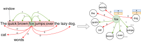
Figure 1. Viewing Word2Vec in Skip-gram model as a graph.

An embedding is a mapping from a dataset $D$ to a vector space ${\rm I\!R}^{N}$ such that elements of $D$ that are related are close to each other in the vector space. The length $N$ of the embedding vectors is typically much smaller than the dimension of $D$.

Many models have been proposed for learning word embeddings (word2vec1, ; word2vec2, ). We will focus on the popular Skip-gram model together with the negative sampling introduced in (word2vec2, ), and explain it here in a form suitable for a graph analytic understanding.

Skip-gram uses a training task where it predicts if a target word $w_{O}$ appears in the context of a center word $w_{I}$. Figure 1 (left) illustrates this for an example sentence, with “fox” as the center word. The context is then defined as the words inside a window of size $c$ (a hyper-parameter) centered on “fox”. In Figure 1 these positive samples are shown in green and have a label of 1. For each positive sample Skip-gram picks $k$ (a hyper-parameter) random words as negative samples and gives them a label of 0.

The Skip-gram model consists of two vectors of size $N$ for each word $w$ in the vocabulary: an embedding vector $e_{w}$ and a training vector $t_{w}$. For a pair of words the model predicts the label with $\sigma(e_{w_{I}}^{T}\cdot t_{w_{O}})$, which should be close to 1 for related words and close to 0 otherwise. The loss term for a sample is then $-\log(1-|y-\sigma(e_{w_{I}}^{T}\cdot t_{w_{O}})|)$, where $y$ is the true label of the sample.

We base the work in this paper on Google’s Word2Vec tool, which uses the Hogwild! parallelization technique. Each thread is given a subset of the corpus and goes through the words in it sequentially (skipping some due to sub-sampling frequent words as described in (word2vec2, )). For each pair of a central word and a target word in its context Word2Vec calculates a gradient using a sum of the loss term for the positive sample itself and loss terms for $k$ negative samples. This gradient is then applied to the model shared by all threads in a racy manner and the thread continues onto the next pair of words.

2.3. Graph Analytics

In typical graph analytics applications, each node has one or more labels, which are updated during algorithm execution until a global quiescence condition is reached. The labels are updated by iteratively applying a computation rule, known as an operator, to the nodes or edges in the graph. The order in which the operator is applied to the nodes or edges is known as the schedule. A node operator takes a node $n$ and updates labels on $n$ or its neighbors, whereas an edge operator takes an edge $e$ and updates labels on source and destination of $e$.

To execute graph applications in distributed-memory, the edges are first partitioned (cusp, ) among the hosts and for each edge on a host, proxies are created for its endpoints. As a consequence of this design, a node might have proxies (or replicas) on many hosts. One of these is chosen as the master proxy to hold the canonical value of the node. The others are known as mirror proxies. Several heuristics exist for partitioning edges and choosing master proxies (partitioningstudy, ).

Most distributed graph analytics systems (powergraph, ; gemini, ; gluon, ) use bulk-synchronous parallel (BSP) execution. Execution is done in rounds of computation followed by bulk-synchronous communication. In the computation phase, every host applies the operator inside its own partition and updates the labels of the local proxies. Thus, different proxies of the same node might have different values. Every host then participates in a global communication phase to synchronize the labels of all proxies. Different proxies of the same node are reconciled by applying a reduction operator, which depends on the algorithm being executed.

3. Distributed Any2Vec

In this section, we first describe the formulation of Any2Vec as a graph application and provide an overview of our distributed GraphAny2Vec (Section 3.1). We then describe the different phases in our approach such as dynamic graph generation and partitioning (Section 3.2), model synchronization (Section 3.3), and communication optimizations (Section 3.4).

3.1. Overview of Distributed GraphAny2Vec

We formulate Any2Vec as a graph problem and call it GraphAny2Vec. Each element in the dataset corresponds to a node in a graph, and the positive and negative samples correspond to edges in the graph with weights 1 and 0 respectively. Figure 1 (right) illustrates this for Word2Vec. Training the Skip-gram model is now a graph analytics application. Each node has two labels — $e$ and $t$ — for embedding and training vectors, respectively, of size $N$. The model corresponds to these labels for all nodes. These labels are initialized randomly and updated during training by applying an edge operator, that takes the source $src$ and destination $dst$ of an edge with weight $w$, computes $\sigma(e_{\texttt{src}}^{T}\cdot t_{\texttt{dst}})$ to predict the relation between the two nodes, and then applies the SGD update rule to $e_{\texttt{src}}$ and $t_{\texttt{dst}}$ so as to minimize the loss function $-\log(1-|w-\sigma(e_{\texttt{src}}^{T}\cdot t_{\texttt{dst}})|)$. The operator is applied to all edges once in each epoch.

Algorithm 1 Execution on each distributed host of GraphAny2Vec.

1:procedure GraphAny2Vec(Corpus $C$, Num. of epochs $R$, Num. of sync rounds $S$, Learning rate $\alpha$)

2:    Let $h$ be the host ID

3:    Stream $C$ from disk to build set of vertices $V$

4:    Read partition $h$ of $C$ that forms the work-list of vertices $W$

5:    for epoch $r$ from 1 to $R$ do

6:         for sync round $s$ from 1 to $S$ do

7:             Let $W_{s}$ be partition $s$ of $W$

8:             Build graph $G$ = ($V$, $E$) where $E$ are samples in $W_{s}$

9:             Compute($G$, $W_{s}$, $\alpha$) $\triangleright$ Updates $G$ and decays $\alpha$

10:             Synchronize($G$) $\triangleright$ Updates $G$

11:         end for

12:    end for

13:end procedure

Algorithm 1 gives a brief overview of our distributed GraphAny2Vec execution. The first step is to construct the set of vertices $V$ (unique words in case of Word2Vec) by making a pass over the training data corpus $C$ on each host in parallel. As $C$ may not fit in the memory of a single host, we stream it from disk to construct $V$. The corpus $C$ is then partitioned (logically) into roughly equal contiguous chunks among hosts. All hosts read their own partition of $C$ in parallel. The list of elements in a given host’s partition of $C$ constitutes the work-list $W$ that the host is responsible for computing Any2Vec on. We introduce a new parameter for controlling the number of synchronization rounds within an epoch. In each epoch on each host, $W$ is partitioned into roughly equal contiguous chunks among the rounds. In each round $s$, positive and negative samples from partition $s$ of $W$ are used to construct the graph. The Any2Vec operator is then applied to all edges in the graph. The operator updates the vertex labels directly and decays the learning rate continuously, as in shared-memory implementation of Any2Vec applications. Then, all hosts participate in a bulk-synchronous communication to synchronize the vertex labels.

We implement GraphAny2Vec in D-Galois (gluon, ), the state-of-the-art distributed graph analytics framework, which consists of the Galois (galois, ) multi-threaded library for computation and the Gluon (gluon, ) communication substrate for synchronization. Galois provides efficient, concurrent data structures like graphs, work-lists, dynamic bit-vectors, etc., which makes it quite straightforward to implement GraphAny2Vec. Gluon incorporates communication optimizations that enable it to scale to a large number of hosts. However, D-Galois only works with static graphs (nodes and edges must not change during algorithm execution), whereas, for Any2Vec applications, edges are sampled randomly and generated. We adapted D-Galois to handle dynamic graph generation efficiently during computation and communication, as explained in Sections 3.2 and 3.4 respectively. Our techniques can be used to modify other distributed graph analytics frameworks and implement GraphAny2Vec in them.

3.2. Graph Generation and Partitioning

As explained in Section 2.2, the Skip-gram model generates positive and negative samples using randomization. Consequently, the samples or edges generated for the same element or node in the corpus in different epochs may be different. As the same edge may not be generated again, one way to abstract this is to consider that the edges are being streamed and each edge is processed only once, even across epochs. Due to this, the graph needs to be constructed in each synchronization round, as shown in Algorithm 1.

The graph can be explicitly constructed in each round. However, this may add unnecessary overheads as each edge is processed only once before the graph is destroyed. More importantly, this does not distinguish between edges (samples) from different occurrences of the same node (element) in the corpus. Consequently, the relative ordering of the edges from different nodes is not preserved. We observed that the accuracy of the model is highly sensitive to the order in which the edges are processed because the learning rate decays after each occurrence of the node is processed. Hence, the key to our graph formulation is that on each host, the schedule of applying operators on edges in GraphAny2Vec must match the order in which samples would be processed in Any2Vec. Note that the work-list $W$ preserves the ordering of element occurrences in the corpus. Thus, GraphAny2Vec generates or streams edges on-the-fly using partition $s$ of $W$ in round $s$, instead of constructing the graph.

Each host generates edges for its own partition of the graph in each synchronization round. In other words, the graph is re-partitioned in every round. By design, each edge is assigned to a unique host. As mentioned in Section 2.3, node proxies are created for the endpoints of edges on a host. The master proxy for each node can be chosen from among its proxies thus created, but this would incur overheads in every round. We instead (logically) partition the nodes once into roughly equal contiguous chunks among the hosts and each host creates master proxies for the nodes in its partition. Proxies for other nodes on the host would be mirror proxies. Each mirror knows the host that has its master using the partitioning of nodes. Each master also needs to know the hosts with its mirrors. We provide two ways to do this: RepModel and PullModel.

In RepModel, each host has proxies for all nodes, so the entire model is replicated on each host. Thus, each host statically knows that every other host has mirror proxies for the masters on it. This allows GraphAny2Vec to assume that an edge between any two nodes can be generated on any host. In PullModel, each hosts makes an inspection pass over $W$ before computation in each round to generate edges and track the nodes that would be accessed during computation. Mirror proxies are then created for the nodes tracked. For each mirror proxy created, the host communicates to the host that has its master (bulk-synchronization).

RepModel requires the entire model to fit in the memory of a host, while PullModel enables handling larger models. On the other hand, PullModel incurs overhead for determining masters and mirrors in each round, whereas RepModel does not. Nonetheless, RepModel and PullModel require different communication to synchronize the model, so we evaluate which of them performs better in Section 5.

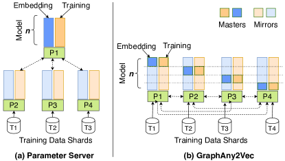
Figure 2. Synchronization of the Skip-gram Model.

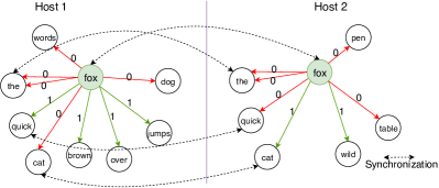
Figure 3. Synchronization of proxies in graph partitions.

3.3. Model Synchronization

Prior work for distributed Word2Vec such as Microsoft’s Distributed Machine Learning Toolkit (DMTK) (DMTK, ) (and other machine learning algorithms) use a parameter server to synchronize the model, as illustrated in Figure 2(a). One of the hosts (say $P1$) is chosen as the parameter server. At the beginning of a round (or a mini-batch), every host receives the updated model from the parameter server. The host then computes that round and sends the model updates to the parameter server. GraphAny2Vec uses a different synchronization model based on D-Galois (gluon, ), as illustrated in Figure 2(b). Abstractly, this can be viewed as a generalization of the parameter server model where each host acts as a parameter server for a partition of the model. In Figure 2(b), $P1$ has the master proxies for the first contiguous chunk or partition of the nodes, $P2$ has the master proxies for the second partition of the nodes, and so on. During synchronization in D-Galois, the mirror proxies send their updated value to the host containing the master, which reduces it and broadcasts it to the hosts containing the mirrors.

Figure 3 shows an example where proxies on two hosts need to be synchronized after computation. Consider the word "fox" that is present on both hosts. It may have different values for the embeddings on both hosts after computation. The reduction operator determines how to synchronize these values and this is a parameter to synchronization in D-Galois. As described in Section 4, averaging or adding the two values may lead to slower convergence, so we introduce a novel way to combine them called Gradient Combiner.

3.4. Communication Optimizations

RepModel-Naive: During synchronization in RepModel, all mirrors on each host can send their updates to their respective masters and the masters can reduce those values and broadcast it to their mirrors. This is similar to communication for dense matrix codes, so can be mapped quite efficiently to MPI collectives. However, in Any2Vec, not all nodes are updated in every round. Consequently, such naive communication would result in redundant communication during both reduce and broadcast phases.

RepModel-Opt: The advantage of D-Galois is that it allows the user to specify the updated nodes and it would transparently handle the sparse communication that would entail. To do this, we maintain a bit-vector that tracks the nodes that were updated in this round. During synchronization, only the updated mirrors are sent to their masters and the masters broadcast their values to the other hosts only if it was updated on any host in that round. This avoids redundant communication during the reduce phase. However, there is still some redundancy during the broadcast phase because the update sent to a mirror might not be accessed by the mirror in the next round. This information remains unknown in RepModel.

PullModel-Base: In PullModel, mirrors are created after inspection only if one of its labels will be accessed on that host. During synchronization, only the mirrors updated in this round are sent to their masters (similar to RepModel-Opt). However, we wait to broadcast after inspection of the next round when new mirrors are created (re-partitioning). During broadcast, all masters must be broadcast whether updated or not, because previous updates may not have been sent to a host if it did not have a mirror during a previous round. This is essentially pulling the model that will be accessed (like in parameter server). While this avoids sending masters to mirrors that do not access it, it may resend masters that have have been updated.

PullModel-Opt: Recall from Section 2.2 that embedding vectors $e$ are accessed only at the source and training vectors $t$ are accessed only at the destination of an edge. If a mirror proxy on a host has only outgoing (or incoming) edges, then it will not access $t$ (or $e$). This is not exploited in PullModel-Base because masters and mirrors are not label-specific in D-Galois. We modified D-Galois to maintain masters and mirrors specific to each label. We also modified our inspection phase to track sources and destinations separately, and create mirrors for $e$ and $t$ respectively. Due to this, masters will broadcast $e$ and $t$ only to those hosts that access each.

4. Gradient Combiner

Section 2 discussed how in the mini-batch approach gradients from multiple training examples are computed in parallel and they are reduced to a single vector by averaging. Although this is a widely-used practice, it does not follow the semantics of the sequential algorithm. Suppose $L_{1}(w)$ and $L_{2}(w)$ are two loss functions corresponding to two training examples. Starting from model $w_{0}$, sequential SGD calculates $w_{1}=w_{0}-\alpha\frac{\partial L_{1}}{\partial w}|_{w_{0}}$ followed by $w_{2}=w_{1}-\alpha\frac{\partial L_{2}}{\partial w}|_{w_{1}}$ where $\alpha$ is a proper learning rate. With forward substituition, $w_{2}=w_{0}-\alpha(\frac{\partial L_{2}}{\partial w}|_{w_{1}}+\frac{\partial L_{1}}{\partial w}|_{w_{0}})$. Alternatively, in a parallel setting, $\frac{\partial L_{1}}{\partial w}|_{w_{0}}$ and $\frac{\partial L_{2}}{\partial w}|_{w_{0}}$ (note that gradients are both at $w_{0}$) are computed and $w$ is updated with $w_{2}^{\prime}=w_{0}-\frac{\alpha}{2}(\frac{\partial L_{1}}{\partial w}|_{w_{0}}+\frac{\partial L_{2}}{\partial w}|_{w_{0}})$. Clearly $w_{2}^{\prime}$ and $w_{2}$ are different because of the averaging effect. (directsum, ) and (sqrtlr, ) have claimed that scaling up the learning rate by the number of parallel processors (or square root of it) closes this gap. However, if $\frac{\partial L_{1}}{\partial w}|_{w_{0}}$ and $\frac{\partial L_{2}}{\partial w}|_{w_{0}}$ are both in the same direction, scaling up the learning rate might cause divergence as we assumed $\alpha$ was properly set for the sequential algorithm. Our Gradient Combiner addresses this problem by adjusting the gradients to each other.

Following the Taylor expansion for $\frac{\partial L_{2}}{\partial w}|_{w_{0}+(w_{1}-w_{0})}$, we have:

(2) $$\begin{split}\frac{\partial L_{2}}{\partial w}\Big{|}_{w_{0}+(w_{1}-w_{0})}&\approx\frac{\partial L_{2}}{\partial w}\Big{|}_{w_{0}}+\frac{\partial^{2}L_{2}}{(\partial w)^{2}}\Big{|}_{w_{0}}\cdot(w_{1}-w_{0})\\ &=\frac{\partial L_{2}}{\partial w}\Big{|}_{w_{0}}-\alpha\frac{\partial^{2}L_{2}}{(\partial w)^{2}}\Big{|}_{w_{0}}\cdot\frac{\partial L_{1}}{\partial w}\Big{|}_{w_{0}}\end{split}$$

where the approximation error is $O(\left\lVert w_{1}-w_{0}\right\rVert^{2})$ which is alternatively $\alpha^{2}O\Big{(}\left\lVert\frac{\partial L_{1}}{\partial w}|_{w_{0}}\right\rVert^{2}\Big{)}$. As the learning rate $\alpha$ gets smaller, the error in Formula 2 shrinks quadratically. Usually as the training of a Any2Vec model progresses, the learning rate is decayed and as a result this error becomes negligible. For the rest of this section, we denote gradients $g_{1}=\frac{\partial L_{1}}{\partial w}|_{w_{0}}$, $g_{2}=\frac{\partial L_{2}}{\partial w}|_{w_{0}}$, $g_{2}^{\prime}=\frac{\partial L_{2}}{\partial w}|_{w_{1}}$ and the Hessian matrix $H_{2}=\frac{\partial^{2}L_{2}}{(\partial w)^{2}}|_{w_{0}}$. Therefore, Equation 2 can be re-written by:

(3) $$g_{2}^{\prime}\approx g_{2}-\alpha H_{2}\cdot g_{1}$$

Equation 3 lets us compute $g_{2}^{\prime}$, however, computing $H_{2}$ is expensive as it is a $n\times n$ matrix where $n$ is the number of parameters in the Any2Vec model. Luckily because Any2Vec has a log-likelihood loss function, $H_{2}$ can be expressed by the outer product of the gradient: $\lambda g_{2}\cdot g_{2}^{T}$ where $\lambda$ is a scalar which depends on $w_{0}$ (msra, ). The error for this approximation gets smaller as $w_{0}\rightarrow w^{*}$ where $w^{*}$ is the optimal model parameters (msra, ; ggt, ). By using Equation 3 and this approximation, $g_{2}^{\prime}$ can be approximated by:

(4) $$g_{2}^{\prime}\approx g_{2}-\alpha\lambda g_{2}\cdot g_{2}^{T}\cdot g_{1}$$

Although Formula 4 makes calculation of $g_{2}^{\prime}$ feasible, finding the right $\lambda$ for every iteration of SGD is overwhelmingly difficult and it is yet another hyper-parameter for the user to tune. However, if $g_{1}$ was orthogonal to $g_{2}$, then $g_{2}^{\prime}$ could have been easily estimated by $g_{2}$. This is the intuition behind Gradient Combiner .

Given that $g_{1}$ and $g_{2}$ are not always orthogonal, we project $g_{1}$ on the orthogonal space of $g_{2}$ to make $g_{1}^{O}$:

(5) $$g_{1}^{O}=g_{1}-\frac{g_{2}^{T}\cdot g_{1}}{\left\lVert g_{2}\right\rVert^{2}}g_{2}$$

$g_{1}^{O}$ has three important properties: (1) $g_{1}^{T}\cdot g_{1}^{O}\geq 0$, (2) $\left\lVert g_{1}^{O}\right\rVert\leq\left\lVert g_{1}\right\rVert$, and (3) $g_{2}^{T}\cdot g_{1}^{O}=0$. It is straight forward to check these properties (see Appendix A.2 for full proof). Suppose $w_{1}^{O}=w_{0}-\alpha g_{1}^{O}$. Then by using the Taylor expansion, we have:

(6) $$L_{1}(w_{1}^{O})=L_{1}(w_{0}-\alpha g_{1}^{O})\approx L_{1}(w_{0})-\alpha g_{1}^{T}\cdot g_{1}^{O}\leq L_{1}(w_{0})$$

where the last inequality comes from property (1). This means that moving in the direction of $g_{1}^{O}$ decays the loss of $L_{1}$. Also, because of property (2) and the fact that the same learning rate as sequential learning rate is used, the approximation in Equation 6 has the same or lower error as the one with $L_{1}(w_{1})$ if we had the Taylor expansion for it (refer to Equation 1). Property (3) and Equation 4 ensure that $\frac{\partial L_{2}}{\partial w}|_{w_{1}^{O}}\approx\frac{\partial L_{2}}{\partial w}|_{w_{0}}=g_{2}$. Let’s assume that sequential SGD uses $g_{1}^{O}$ to get to $w_{1}^{O}=w_{0}-\alpha g_{1}^{O}$ followed by computing $\frac{\partial L_{2}}{\partial w}|_{w_{1}^{O}}$ which can be approximated by $g_{2}$ to get to $w_{2}^{O}=w_{1}^{O}-\alpha g_{2}$. By forward substituition:

(7) $$w_{2}^{O}=w_{0}-\alpha(g_{2}+g_{1}^{O})=w_{0}-\alpha\Bigg{(}g_{2}+g_{1}-\frac{g_{2}^{T}\cdot g_{1}}{\left\lVert g_{2}\right\rVert^{2}}g_{2}\Bigg{)}$$

Therefore, the direction Gradient Combiner ($GC(g_{1},g_{2})$ for short) uses to move is:

(8) $$GC(g_{1},g_{2})=g_{2}+g_{1}-\frac{g_{2}^{T}\cdot g_{1}}{\left\lVert g_{2}\right\rVert^{2}}g_{2}$$

which allows computation of $g_{1}$ and $g_{2}$ in parallel. Note that our gradient combiner requires slightly more computation than averaging but as we will show in Section 5, this overhead is negligible.

The magnitude of $GC(g_{1},g_{2})$ depends on how parallel or orthogonal $g_{1}$ and $g_{2}$ are to each other. In the parallel case, $g_{1}^{O}$ becomes smaller and therefore, moving in the direction of $g_{1}^{O}$ decays the loss value of $L_{1}$ slower than $g_{1}$. However, as we will show in Section 5, the gradients all start parallel to each other in the begining of the training as they all point in the same general direction and later in the training they become more orthogonal. This means that Gradient Combiner conservatively takes small steps in the begining of the training and larger ones as the training progresses.

Gradient Combiner extends to combining $k$ gradients as well where gradients are combined sequentially manner as discussed in Section 3.3 ($GC(g_{1},\dots,g_{k})=GC(g_{k},\dots,GC(g_{3},GC(g_{2},g_{1}))\dots)$). Appendix A.3 proves the convergence of Gradient Combiner in expectation.

The effectiveness of Gradient Combiner depends on the degree to which the gradients are orthogonal. We define

(9) $$O(g_{1},g_{2})=\frac{\left\lVert GC(g_{1},g_{2})^{2}\right\rVert}{\left\lVert g_{1}\right\rVert^{2}+\left\lVert g_{2}\right\rVert^{2}}=\frac{\left\lVert g_{1}^{O}+g_{2}\right\rVert^{2}}{\left\lVert g_{1}\right\rVert^{2}+\left\lVert g_{2}\right\rVert^{2}}$$

as a notion for orthogonality of $g_{1}$ and $g_{2}$. Note that because of property (3) $g_{1}^{O}$ and $g_{2}$ are orthogonal and $\left\lVert g_{1}^{O}+g_{2}\right\rVert^{2}=\left\lVert g_{1}^{O}\right\rVert^{2}+\left\lVert g_{2}\right\rVert^{2}$ thanks to Pythagorean theorem. Therefore, $\left\lVert g_{1}^{O}+g_{2}\right\rVert^{2}=\left\lVert g_{1}^{O}\right\rVert^{2}+\left\lVert g_{2}\right\rVert^{2}\leq\left\lVert g_{1}\right\rVert^{2}+\left\lVert g_{2}\right\rVert^{2}$ which concludes that $t\leq 1$ and equality is met only when $g_{1}$ and $g_{2}$ are orthogonal. On the other hand, if $g_{1}=g_{2}$, $g_{1}^{O}$ becomes zero and $O(g_{1},g_{2})=\frac{1}{2}$. This can be similarly expanded to $k$ gradients $O(g_{1},\dots,g_{k})=\frac{GC(g_{1},\dots,g_{k})^{2}}{\sum_{i}\left\lVert g_{i}\right\rVert^{2}}$. Similarly for $k$ gradients, orthogonality is $1$ when they are all orthogonal and $\frac{1}{k}$ when they are all the same.

5. Evaluation

Table 1. Datasets and their properties.

Applications	Datasets	Vocabulary Words	Training Words	Size	Labels
Word2Vec (Text)	1-billion	399.0K	665.5M	3.7GB	N/A
	news	479.3K	714.1M	3.9GB	N/A
	wiki	2759.5K	3594.1M	21GB	N/A
Vertex2Vec (Graph)	BlogCatalog	10.3K	4.1M	0.02GB	39
	Flickr	80.5K	32.2M	0.18GB	195
	Youtube	1138.5K	455.4M	2.8GB	47

Table 2. Word2Vec training time (hours) on a single host.

Dataset	W2V	GEM	DMTK(AVG)	GW2V(GC)
1-billion	4.24	4.39	4.21	3.98
news	4.45	4.66	4.28	4.51
wiki	20.49	OOM	25.43	22.34

Table 3. Word2Vec accuracy (semantic, syntactic, and total) of different frameworks relative to W2V.

	Framework	1-billion	news	wiki
Semantic	W2V (1 Host)	75.86$\pm$0.07	70.79$\pm 0.54$	79.10$\pm 0.31$
	GEN (1 Host)	-0.22	-0.22	OOM
	DMTK (1 Host)	-13.79	-18.43	-7.46
	DMTK(AVG) (32 Hosts)	-57.36	-57.15	-34.39
	DMTK(GC) (32 Hosts)	-10.93	-17	-5.17
	GW2V (1 Host)	+0.07	-0.08	+0.26
	GW2V(AVG) (32 Hosts)	-7.00	-9.15	-4.03
	GW2V(GC) (32 Hosts)	+0.21	+0.07	-0.17
Syntactic	W2V (1 Host)	50.0$\pm 0.18$	50.0$\pm 0.26$	49.22$\pm 0.12$
	GEN (1 Host)	-0.14	-0.12	OOM
	DMTK (1 Host)	-1.89	-0.67	-3.11
	DMTK(AVG) (32 Hosts)	-24.89	-25.11	-23.11
	DMTK(GC) (32 Hosts)	-3.56	-1.78	-1.44
	GW2V (1 Host)	-0.37	0.0	-0.12
	GW2V(AVG) (32 Hosts)	-4.89	-4.11	-7.55
	GW2V(GC) (32 Hostss)	+0.10	+0.11	+0.18
Total	W2V (1 Host)	72.36$\pm 0.21$	69.21$\pm 0.42$	74.10$\pm 0.42$
	GEN (1 Host)	+0.0	-0.14	OOM
	DMTK (1 Host)	-11.65	-15.42	-3.03
	DMTK(AVG) (32 Hosts)	-51.29	-51.71	-32.03
	DMTK(GC) (32 Hosts)	-9.86	-14.78	-5.24
	GW2V (1 Host)	-0.14	-0.28	+0.1
	GW2V(AVG) (32 Hosts)	-6.79	-9.28	-5.17
	GW2V(GC) (32 Hostss)	+0.14	+0.29	-0.17

We implement distributed Word2Vec and Vertex2Vec in our GraphAny2Vec framework, and we refer to these applications as GraphWord2Vec (GW2V) and GraphVertex2Vec (GV2V) respectively. First, we compare these with the state-of-the-art third-party implementations (Section 5.1). We then analyze the impact of our Gradient Combiner (Section 5.2) and communication optimizations (Section 5.3). Our evaluation methodology is described in detail in Appendix A.1.

5.1. Comparing With The State-of-The-Art

Word2Vec: We compare GW2V with distributed-memory implementation DMTK (DMTK, ) and shared-memory implementations, W2V (word2vec2, ) and GEN (gensim, ). Table 2 compares their training time on a single host. Figure 6 shows the speedup of both GW2V and DMTK on 32 hosts over W2V on 1 host. Note that averaging (AVG) and our Gradient Combiner (GC) methods are used to combine gradients during inter-host synchronization, so they have no impact on a single host.

Performance: We observe that for all datasets on a single host, the training time of GW2V is similar to that of W2V, GEN, and DMTK. GW2V scales up to 32 hosts and speeds up the training time by $\sim 13\times$ on average over 1 host. In comparison with distributed DMTK on 32 hosts, which uses parameter servers for synchronization , GW2V is $\sim 2\times$ faster on average for all datasets. Figure 6 also shows that there is negligible performance between using AVG and using GC to combine gradients in both DMTK and GW2V. Training wiki using GW2V takes only 1.9 hours, which saves 18.6 hours and 1.5 hours compared to training using W2V and DMTK respectively.

To understand the performance differences between DMTK and GW2V better, Figure 6 shows the breakdown of their training time into 3 phases: inspection, computation, and (non-overlapped) communication. Firstly, GW2V’s inspection phase as well as serialization and de-serialization during synchronization are parallel using D-Galois (galois, ; gluon, ) parallel constructs and concurrent data-structures such as bit-vectors, work-lists, etc., whereas these phases are sequential in DMTK as it uses non-concurrent data-structures such as set and vector provided by the C++ standard template library. Moreover, in GW2V, hosts can update their masters in-place. This is not possible in DMTK as workers on each host have to fetch model parameters from servers on the same host to update, incurring overhead for additional copies. Secondly, DMTK communicates much higher volume ($\sim 3.5\times$) than GraphWord2Vec. GW2V memoizes the node IDs exchanged during inspection phase and sends only the updated values during broadcast and reduction. In contrast, DMTK sends the node IDs along with the updated values to the parameter servers during both broadcast and reduction. In addition, GraphWord2Vec inspection precisely identifies both the positive and negative samples required for the current round. DMTK, on the other hand, only identifies precise positive samples, and builds a pool for negative samples. During computation, negative samples are randomly picked from this pool. The entire pool is communicated from and to the parameter servers, although some of them may not be updated, leading to redundant communication.

Table 4. Vertex2Vec training time (sec) of DeepWalk on 1 host vs. GraphVertex2Vec (GV2V) on 16 hosts.

Dataset	DeepWalk	GV2V	Speedup
BlogCatalog	115.3	28.8	4.0x
Flickr	976.7	183.1	5.3x
Youtube	11589.2	2226.2	5.2x

Table 5. Vertex2Vec accuracy (Macro F1 and Micro F1) of GV2V on 16 hosts relative to DeepWalk on 1 host.

		% Labeled Nodes	30%	60%	90%
Micro-F1	BlogCatalog	Deepwalk	34.0	37.2	38.4
		GV2V	-0.1	+0.1	+0.7
	Flickr	Deepwalk	38.6	40.4	41.1
		GV2V	+0.1	-0.1	-0.2
Macro-F1	BlogCatalog	Deepwalk	34.1	37.2	38.4
		GV2V	-0.3	+0.1	+0.7
	Flickr	Deepwalk	26.5	28.7	29.5
		GV2V	+0.1	-0.1	+0.3

Accuracy: Table 3 compares the accuracies (semantic, syntactic, and total) for all frameworks on 1 and 32 hosts relative to the accuracies achieved by W2V. On a single host, GW2V is able to achieve accuracies (semantic, syntactic and total) comparable to W2V. DMTK on a single host is less accurate due to implementation differences in the Skip-gram model training; DMTK only updates learning rate between mini-batches, whereas others continuously degrade learning rate, and DMTK uses a different strategy to choose negative samples as described earlier. On 32 hosts, DMTK(AVG) has terrible accuracy and GW2V(AVG) has poor accuracy. GC significantly improves the accuracies over AVG for both DMTK and GW2V. DMTK(GC) improves semantic by 37.91%, syntactic by 22.09%, and total by 34.79% to match its own single host accuracy. GW2V(GC) improves all accuracies to match that of W2V.

Vertex2Vec: Table 4 compares the training time of DeepWalk (deepwalk, ) on a single host with our GV2V on 16 hosts. We observe that for all datasets, GraphVertex2Vec can train the model $\sim 4.8\times$ faster on average. Similar to GraphWord2Vec, this speedup does not come at the cost of the accuracy, as shown in Table 5, which shows the Micro-F1 and Macro-F1 score with 30$\%$, 60$\%$, and 90$\%$ labeled nodes.

Discussion: GraphAny2Vec significantly speeds up the training time for Word2Vec and Vertex2Vec applications by distributing the computation across the cluster without sacrificing the accuracy. Reduced training time also accelerates the process of improving the training algorithms as it allows application designers to make more end-to-end passes in a short duration of time.

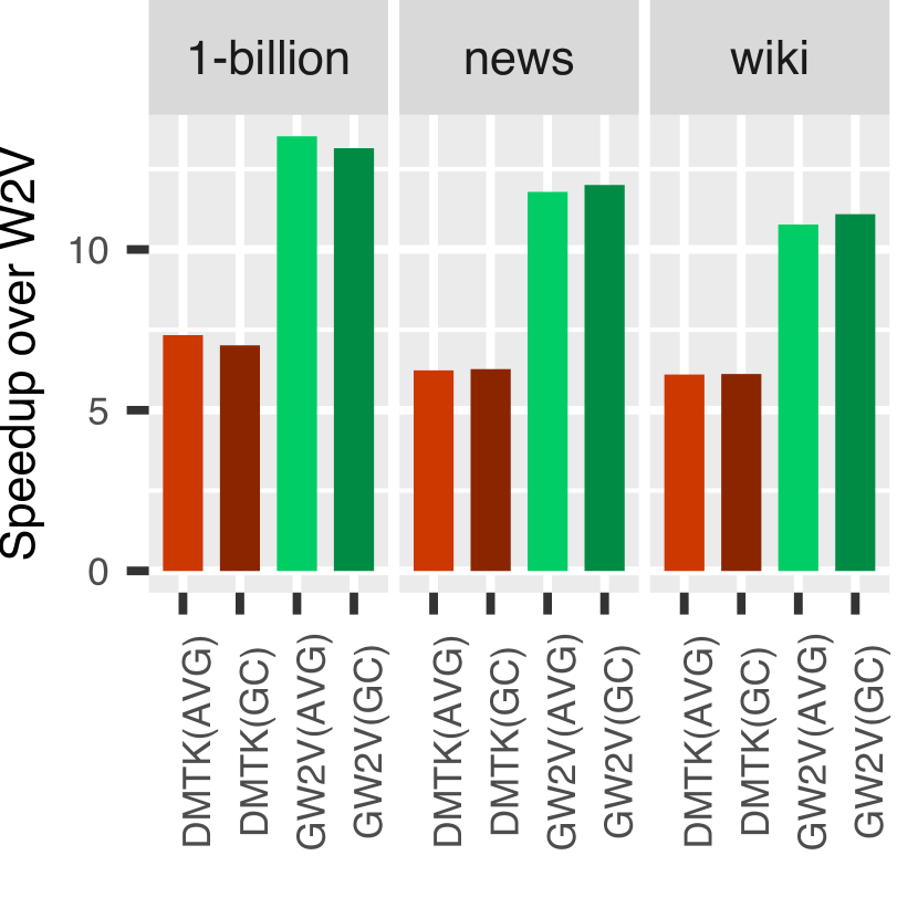
Figure 4. Speedup of DMTK and GW2V on 32 hosts over W2V on 1 host.

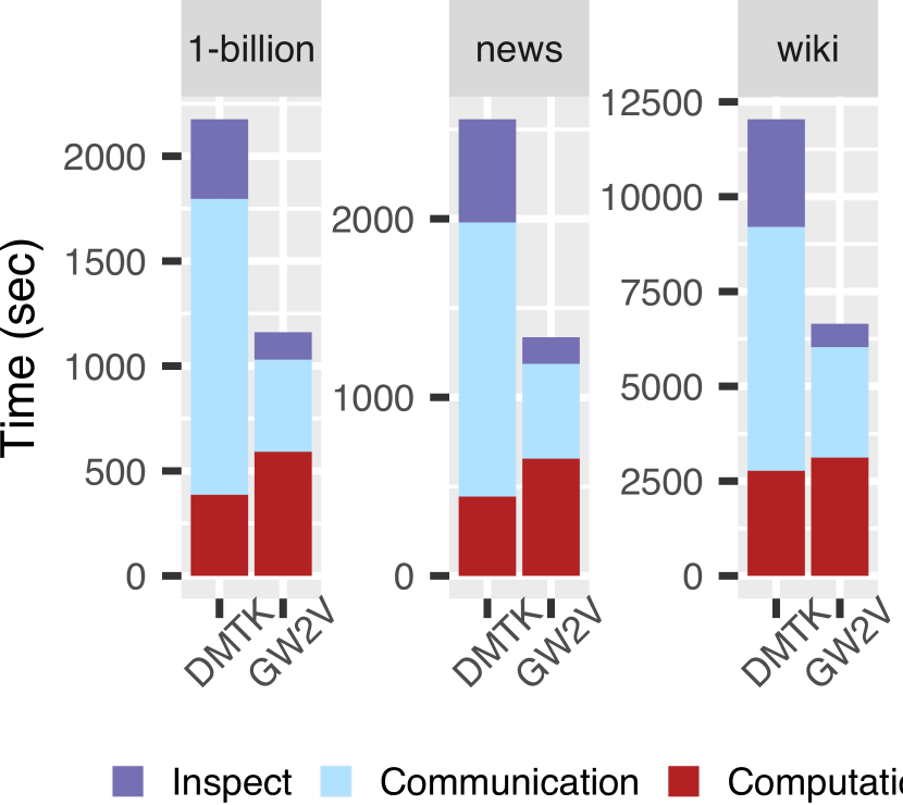
Figure 5. Breakdown of training time of DMTK(GC) and GW2V(GC) on 32 hosts.

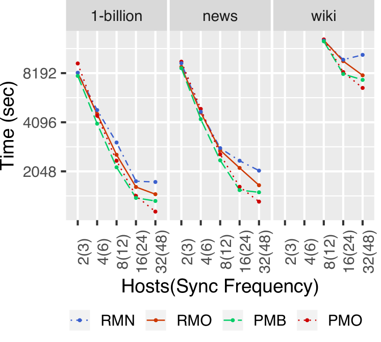
Figure 6. Strong scaling of GW2V (RMN: RepModel-Naive, RMO: RepModel-Opt, PMB: PullModel-Base, PMO: PullModel-Opt).

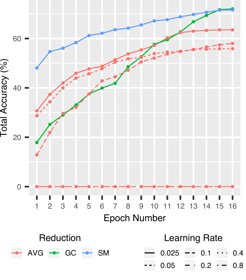
Figure 7. Accuracy of GW2V after each epoch for 1-billion dataset on 1 host (SM) and on 32 hosts using GC and AVG.

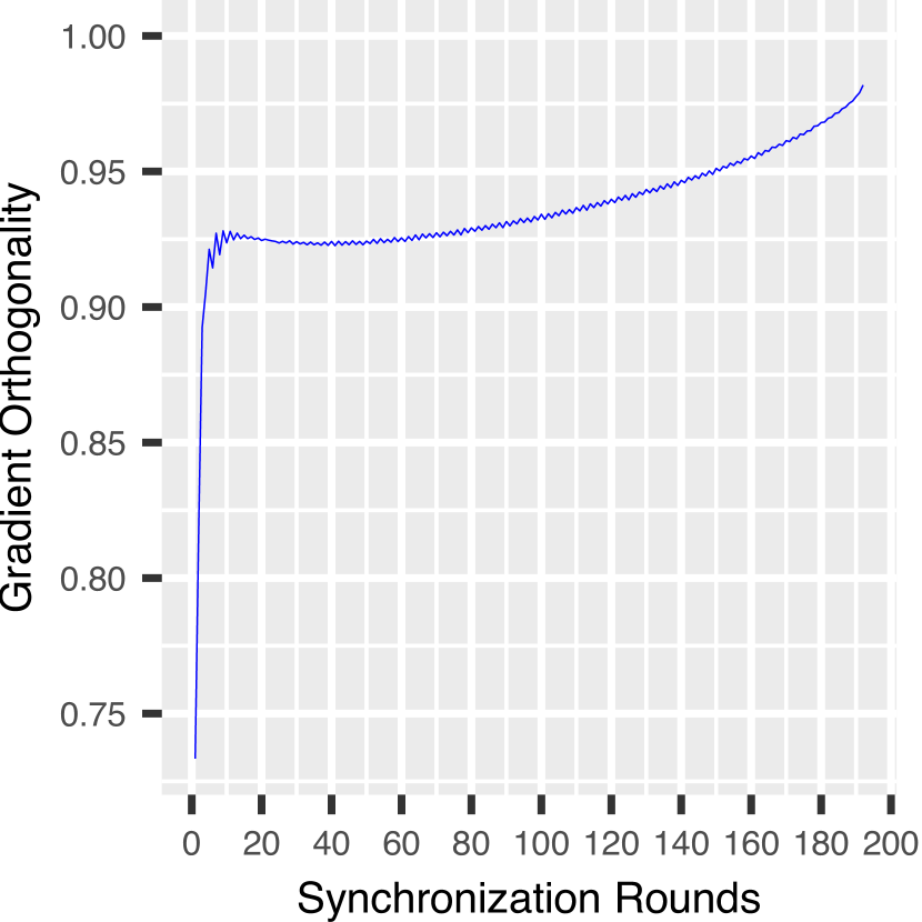
Figure 8. GW2V for 1-billion dataset on 32 hosts: % of gradients of a node that are orthogonal to each other in each epoch.

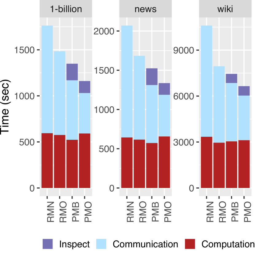
Figure 9. Breakdown of training time of GW2V with different communication schemes on 32 hosts.

5.2. Impact of Gradient Combiner (GC)

If time were not an issue, all machine learning algorithms would run sequentially. A sequential SGD is simple to tune and converges fast. Unfortunately, it is slow. A point $(x,y)$ on Figure 9 denotes the total accuracy ($y$) as a function of epoch ($x$). The blue line (SM) shows the accuracy of GW2V on a single shared-memory host. It clearly converges to a high accuracy quickly. In contrast, the red lines plot accuracy of distributed GW2V that uses averaging the gradients (AVG) with different learning rates on 32 hosts. The learning rate of 0.025 is the same as SM while the learning rate of 0.8 is 32 times larger. The former converges slowly while the latter does not converge at all (accuracy is 0) because the learning rate is too large. Finally, the green line plots accuracy of distributed GW2V that uses GC and 0.025 as the learning rate on 32 hosts. GC has no problem meeting the accuracy of the sequential algorithm. In addition to providing the same accuracy as SM, it is $12\times$ times faster on 32 hosts than SM. Not having to tune the learning rate and still getting accuracy at scale is a significant qualitative contribution of our work as tuning is a difficult task, in general.

In each round, we count the number of gradients that are being combined and the percentage of them that are orthogonal to each during combining. Figure 9 shows this percentage as function of the rounds. In later rounds, more and more gradients are orthogonal to each other. As explained in Section 4, GC is more effective when the gradients are orthogonal. This is validated by the increase in accuracy for GC in later epochs in Figure 9.

Synchronization Rounds: Gradient Combiner (GC) improves the accuracies significantly but in order to get accuracies comparable to shared-memory implementations, the number of synchronization rounds in each epoch is an important knob to tune. We observe that accuracies improve as we increase the number of synchronization rounds within an epoch for both GC and AVG. Nonetheless, accuracies show more improvement for GC (for example, semantic: 3.07%, syntactic: 3.99% and total: 3.36% when synchronization frequency is increased from 12 to 48 on 32 hosts) as opposed to AVG, which shows very little change in accuracies with synchronization rounds. In general, we have observed that in order to maintain the desired accuracy, the synchronization frequency needs to be increased (roughly) linearly with the number of hosts. We have followed this rule of thumb in all our experiments.

5.3. Impact of Communication Optimizations

Figure 6 shows the strong scaling of GraphWord2Vec with different communication optimizations (described in section 3.4): RepModel-Naive (RMN), RepModel-Opt (RMO), PullModel-Base (PMB), and PullModel-Opt (PMO). The 3 latter variants scale well up to 32 machines.

For 1-billion dataset, RepModel-Naive gives $4.7\times$ speedup on 32 hosts over 2 hosts. RepModel-Opt, which uses D-Galois to only communicate the updated values for both reduction and broadcast, gives a speedup of $5.5\times$ by reducing the communication volume. RepModel-Opt shows 16% improvement over RepModel-Naive on 32 hosts, showing that RepModel-Opt is able to exploit the sparsity in the communication. The benefits of RepModel-Opt over RepModel-Naive increases with the number of hosts for two main reasons: (a) synchronization frequency doubles with the number of hosts, thus communicating more data, and (b) as training data gets divided among hosts, sparsity in the updates increase.

PullModel-Base not only avoids replication of the model on all hosts (thus can fit bigger models), but helps reduce communication volume over RepModel-Opt by only broadcasting model parameters required by hosts for the next round. PullModel-Opt further reduces communication volume by taking into consideration the location of access as well: it only broadcasts embedding vector for sources and training vector for destinations. These benefits come with an additional overhead of inspection phase before every synchronization round, but our evaluation shows that these overheads are offset by runtime improvements due to communication volume reduction. PullModel-Opt yields an average speedup of $8.1\times$ on 32 hosts over 2 hosts and is $\sim 20.6\%$ on average faster than RepModel-Opt for all text datasets on 32 hosts.

Figure 9 shows the breakdown of the training time into inspection, computation, and communication time of the variants on 32 hosts. It is clear that all variants have similar computation time. RepModel-Opt communicates $\sim 2\times$ less communication volume on average as opposed to RepModel-Naive, thus improving the overall runtime. PullModel-Opt not only allows to train bigger models, it also further reduces communication volume by $\sim 11\%$ on average over RepModel-Opt by only broadcasting specific vectors to the proxies to be used in the next batch.

Summary: PullModel-Opt in GraphAny2Vec always performs better than the other variants by reducing the communication volume. These improvements are expected to grow as we scale to bigger datasets and number of hosts. Hence, PullModel-Opt not only allows one to train bigger models, but also gives the best performance.

6. Related Work

Many different types of models have been proposed in the past for estimating continuous representations of words, such as Latent Semantic Analysis (LSA) and Latent Dirichlet Allocation (LDA). However, distributed representations of words learned by neural networks are shown to perform significantly better than LSA (zhila2013combining, ; mikolov2013linguistic, ) and LDA is computationally very expensive on large data sets. Mikolov et al. (word2vec1, ) proposed two simpler model architectures for computing continuous vector representations of words from very large unstructured data sets, known as Continuous Bag-of-Words (CBOW) and Skip-gram (SG). These models removed the non-linear hidden layer and hence avoid dense matrix multiplications, which was responsible for most of the complexity in the previous models.

CBOW is similar to the feedforward Neural Net Language Model (NNLM) (nnlm, ), where the non-linear hidden layer is removed and the projection layer is shared for all words. All words get projected into the same position and their vectors are averaged.

SG on the other hand unlike CBOW, instead of predicting the current word based on the context, tries to maximize classification of a word based on another word within a sentence. Later Mikolov et al. (word2vec2, ) further introduced several extensions, such as using hierarchical softmax instead of full softmax, negative sampling, subsampling of frequent words, etc., to SG model that improves both the quality of the vectors and the training speed.

Our work adapts the algorithm from this later work (word2vec2, ) for distribution. This work, together with many current implementations (gensim, ) are designed to run on a single machine but utilizing multi-threaded parallelism. Our work is motivated by the fact that these popularly used implementations take days or even weeks to train on large training corpus. Prior works on distributing Word2Vec either use synchronous data-parallelism (Deeplearning4j, ; Sparkword2vec, ; pword2vec, ) or parameter-server style asynchronous data parallelism (DMTK, ). However, they perform communication after every mini-batch, which is prohibitively expensive in terms of network bandwidth. Our design was motivated by the need to use commodity machines and network available on public clouds. Our approach communicates infrequently and uses our novel Gradient Combiner to overcome the resulting staleness.

Ordentlich et al. (Ordentlich16, ) propose a different method designed for models that do not fit in the memory of a single machine. They partition the model vertically with each machine containing part of the embedding and training vector for each word. These partitions compute partial dot products locally but communicate to compute global dot products. For all the publicly available benchmarks we could find, the models fit in the memory in our machines. Nevertheless, our design allows for horizontal partitioning of large models if such a need arises in the future.

7. Conclusions

GraphAny2Vec substantially speeds up the training time for Any2Vec applications by distributing the computation across the cluster without sacrificing the accuracy. Reduced training time also accelerates the process of improving the training algorithms as it allows application designers to make more end-to-end passes in a short duration of time. GraphAny2Vec thus enables more explorations of Any2Vec applications in areas such as natural language processing, network analysis, and code analysis.

Gradient Combiner is the key to GraphAny2Vec’s accuracy. It significantly improves accuracy of SGD compared to the traditional averaging method of combining gradients, even in third-party distributed implementations. Gradient Combiner may also be useful in distributed training of other machine learning applications.

Appendix A Appendix

A.1. Experimental Methodology

Hardware: All our experiments were conducted on the Stampede2 cluster at the Texas Advanced Computing Center using up to 32 Intel Xeon Platinum 8160 (“Skylake”) nodes, each with 48 cores with clock rate 2.1Ghz, 192GB DDR4 RAM, and 32KB L1 data cache. Machines in the cluster are connected with a 100Gb/s Intel Omni-Path interconnect. Code is compiled with g++ 7.1 and MPI mvapich2/2.3.

Datasets: Table 1 lists the training datasets used for our evaluation: text datasets for Word2Vec and graph datasets for Vertex2Vec. These datasets have different vocabulary sizes (# unique words or vertices), total training corpus size (# occurrences of words or vertices), and sizes on disk. Prior Word2Vec and Vertex2Vec publications used the same datasets. The wiki (21GB) and Youtube (2.8GB) datasets are the largest text and graph datasets respectively. We used DeepWalk [23] for generating training corpus for Vertex2Vec by performing 10 random walks each of length 40 from all vertices of the graph. We limit our Word2Vec and Vertex2Vec evaluation to 32 and 16 hosts of Stampedes respectively because these datasets do not scale beyond that. We report the accuracy and the training (or execution) time for all frameworks on these datasets, excluding preprocessing time, as an average of three distinct runs.

Shared-memory third-party implementations: We evaluated the Skip-gram [19] (with negative sampling) training model for both Word2Vec and Vertex2Vec. We compared GraphWord2Vec (GW2V) with the state-of-the-art shared-memory Word2Vec implementations, the original C implementation (W2V) [19] as well as the more recent Gensim (GEN) [26] python implementation. We also compared our GraphVertex2Vec (GV2V) with the state-of-the-art shared-memory Vertex2Vec framework, DeepWalk [23] (both DeepWalk and Node2Vec [12] use Gensim’s [26] Skip-gram model).

Distributed-memory third-party implementations: We compared GraphWord2Vec with the state-of-the-art distributed-memory Word2Vec from Microsoft’s Distributed Machine Learning Toolkit (DMTK) [27], which is based on the parameter server model. The model is distributed among parameter server hosts. During execution, hosts acting as workers request the required model parameters from the servers and send model updates back to the servers. Each host in the cluster acts as both server and worker, and it is the only configuration possible. DMTK uses OpenMP for parallelization within a host (GraphWord2Vec uses Galois [21] for parallelization within a host). Both GraphWord2Vec and DMTK use MPI for communication between hosts. We modified DMTK to include a runtime option of configuring the number of synchronization rounds. DMTK uses averaging as the reduction operation to combine the gradients. We refer to this as DMTK(AVG). We also implemented our Gradient Combiner in DMTK and we call this DMTK(GC). There are no prior distributed implementations of Vertex2Vec. Unless otherwise specified, GW2V and GV2V uses GC to combine gradients and use PullModel-Opt communication optimization.

Hyper-parameters: We used the hyper-parameters suggested by [19], unless otherwise specified: window size of 5, number of negative samples of 15, sentence length of 10K, threshold of $10^{-4}$ for Word2Vec and $0$ for Vertex2Vec for down-sampling the frequent words, and vector dimensionality $N$ of 200. All models were trained for 16 epochs. For distributed frameworks, GV2V, GW2V, and DMTK, we compared 2 gradient combining methods: Averaging (AVG) (default for distributed training of Any2Vec applications) and our novel Gradient Combiner (GC) method. Unless otherwise specified, GV2V, GW2V, and DMTK use the same number of synchronization rounds: 1 for 1 host, 3 for 2 hosts, 6 for 4 hosts, 12 for 8 hosts, 24 for 16 hosts, and 48 for 32 hosts. Note that the default for DMTK is 1 synchronization round for any number of hosts, but this yields very low accuracy, so we do not report these results.

Accuracy: In order to measure the accuracy of trained models of Word2Vec on different datasets, we used the analogical reasoning task outlined by original Word2Vec [19] paper. We evaluated the accuracy using scripts and question-words.txt provided by the Word2Vec code base. Question-words.txt consists of analogies such as "Athens" : "Greece" :: "Berlin" : ?, which are predicted by finding a vector $x$ such that embedding vector($x$) is closest to embedding vector("Athens") - vector("Greece") + vector("Berlin") according to the cosine distance. For this particular example the accepted value of $x$ is "Germany". There are 14 categories of such questions, which are broadly divided into 2 main categories: (1) the syntactic analogies (such as "calm" : "calmly" :: "quick" : "quickly") and (2) the semantic analogies such as the country to capital city relationship. We report semantic, syntactic, and total accuracy averaged over all the 14 categories of questions. For Vertex2Vec , we measured Micro-F1 and Macro-F1 scores using scoring scripts provided by DeepWalk [23].

A.2. Proof of Properties of Gradient Combiner

The three properties of Gradient Combiner are (1) $g_{1}^{T}\cdot g_{1}^{O}\geq 0$, (2) $\left\lVert g_{1}^{O}\right\rVert\leq\left\lVert g_{1}\right\rVert$, and (3) $g_{2}^{T}\cdot g_{1}^{O}=0$ where $g_{1}^{O}=g_{1}-\frac{g_{2}^{T}\cdot g_{1}}{\left\lVert g_{2}\right\rVert^{2}}g_{2}$. For the proof, assume that the angle between $g_{1}$ and $g_{2}$ is $\theta$.

Property (1): $g_{1}^{T}\cdot g_{1}^{O}\geq 0$.

(10) $$\begin{split}g_{1}^{T}\cdot g_{1}^{O}&=g_{1}^{T}\cdot(g_{1}-\frac{g_{2}^{T}\cdot g_{1}}{\left\lVert g_{2}\right\rVert^{2}}g_{2})=\left\lVert g_{1}\right\rVert^{2}-\frac{g_{2}^{T}\cdot g_{1}}{\left\lVert g_{2}\right\rVert^{2}}g_{1}^{T}\cdot g_{2}\\ &=\left\lVert g_{1}\right\rVert^{2}-\frac{\left\lVert g_{1}\right\rVert^{2}\left\lVert g_{2}\right\rVert^{2}\cos^{2}\theta}{\left\lVert g_{2}\right\rVert^{2}}=\left\lVert g_{1}\right\rVert^{2}\sin^{2}\theta\geq 0\end{split}$$

Property (2): $\left\lVert g_{1}^{O}\right\rVert\leq\left\lVert g_{1}\right\rVert$.

(11) $$\begin{split}\left\lVert g_{1}^{O}\right\rVert^{2}&=\left\lVert g_{1}-\frac{g_{2}^{T}\cdot g_{1}}{\left\lVert g_{2}\right\rVert^{2}}g_{2}\right\rVert^{2}\\ &=\left\lVert g_{1}\right\rVert^{2}+\frac{(g_{2}^{T}\cdot g_{1})^{2}}{\left\lVert g_{2}\right\rVert^{4}}\left\lVert g_{2}\right\rVert^{2}-2\frac{g_{2}^{T}\cdot g_{1}}{\left\lVert g_{2}\right\rVert^{2}}g_{1}^{T}\cdot g_{2}\\ &=\left\lVert g_{1}\right\rVert^{2}+\frac{(g_{2}^{T}\cdot g_{1})^{2}}{\left\lVert g_{2}\right\rVert^{2}}-2\frac{(g_{2}^{T}\cdot g_{1})^{2}}{\left\lVert g_{2}\right\rVert^{2}}=\left\lVert g_{1}\right\rVert^{2}-\frac{(g_{2}^{T}\cdot g_{1})^{2}}{\left\lVert g_{2}\right\rVert^{2}}\\ &=\left\lVert g_{1}\right\rVert^{2}-\frac{\left\lVert g_{1}\right\rVert^{2}\left\lVert g_{2}\right\rVert^{2}\cos^{2}\theta}{\left\lVert g_{2}\right\rVert^{2}}=\left\lVert g_{1}\right\rVert^{2}-\left\lVert g_{1}\right\rVert^{2}\cos^{2}\theta\\ &=\left\lVert g_{1}\right\rVert^{2}\sin^{2}\theta\leq\left\lVert g_{1}\right\rVert^{2}\end{split}$$

Property (3): $g_{2}^{T}\cdot g_{1}^{O}=0$.

(12) $$\begin{split}g_{2}^{T}\cdot g_{1}^{O}&=g_{2}^{T}\cdot(g_{1}-\frac{g_{2}^{T}\cdot g_{1}}{\left\lVert g_{2}\right\rVert^{2}}g_{2})=g_{2}^{T}\cdot g_{1}-\frac{g_{2}^{T}\cdot g_{1}}{\left\lVert g_{2}\right\rVert^{2}}\left\lVert g_{2}\right\rVert^{2}\\ &=g_{2}^{T}\cdot g_{1}-g_{2}^{T}\cdot g_{1}=0\end{split}$$

A.3. Gradient Combiner (GC) Convergence Proof

[24] discusses the requirements for a training algorithm to converge to its optimal answer. Here we will present a simplied version of Theorem 1 and Corollary 1 from [24].

Suppose that there are $N$ training examples for a model with loss functions $L_{1}(w),\dots,L_{N}(w)$ where $w$ is the model parameter and $w_{0}$ is the initial model. Define $L(w)=\frac{1}{N}\sum_{i}L_{i}(w)$. Also assume that $w^{*}$ is the optimal model where $L(w^{*})\leq L(w)$ for all $w$s. A training algorithm is pseudogradient if:

• It is an iterative algorithm where $w_{i+1}=w_{i}-\alpha_{i}h_{i}$ where $h_{i}$ is a random vector and $\alpha_{i}$ is a scalar.

• $\forall\epsilon\exists\delta:E(h_{i})^{T}\cdot\nabla L(w)\geq\delta>0$ where $L(w)\geq L(w^{*})+\epsilon$ and $w^{*}$ is the optimal model.

• $E(\left\lVert h_{i}\right\rVert^{2})<C$ where $C$ is a constant.

• $\forall i:\alpha_{i}\geq 0$, $\sum_{i}\alpha_{i}=\inf$, and $\sum_{i}\alpha_{i}^{2}<\inf$.

The following Theorem is taken from [24].

Theorem A.1.

A pseudogradient training algorithm converges to the optimal model $w^{*}$.

As a reminder, $GC(g_{1},g_{2})=g_{2}+g_{1}-\frac{g_{2}^{T}\cdot g_{1}}{\left\lVert g_{2}\right\rVert^{2}}g_{2}$ and for $k$ gradients, $GC(g_{1},\dots,g_{k})=GC(g_{k},\dots,GC(g_{3},GC(g_{2},g_{1}))\dots)$. Suppose $G(w_{i})=\{\frac{\partial L_{1}}{\partial w}|_{w_{i}},\dots,\frac{\partial L_{N}}{\partial w}|_{w_{i}}\}$ is a random variable distribution of the gradients at $w_{i}$.

Theorem A.2.

Suppose $h_{i}=GC(g_{1},\dots,g_{k})$ where $g_{1},\dots,g_{k}$ are $k$ independently chosen gradients from $G(w_{i})$. $h_{i}$ is pseudogradient.

Proof.

To facilitate the proof of the pseudogradient properties of $h_{i}$, we rewrite GC formula as follows:

(13) $$\begin{split}GC(g_{1},g_{2})&=g_{2}+g_{1}-\frac{g_{2}^{T}\cdot g_{1}}{\left\lVert g_{2}\right\rVert^{2}}g_{2}=g_{1}+g_{2}-\frac{g_{2}\cdot g_{2}^{T}}{\left\lVert g_{2}\right\rVert^{2}}g_{1}\\ &=\Big{(}I-\frac{g_{2}\cdot g_{2}^{T}}{\left\lVert g_{2}\right\rVert^{2}}\Big{)}g_{1}+g_{2}\end{split}$$

where $\frac{g_{2}\cdot g_{2}^{T}}{\left\lVert g_{2}\right\rVert^{2}}$ is a rank-1 matrix.

First by induction, we prove that $E(GC(g_{1},\dots,g_{k}))$ and $\nabla L(w_{i})$ have a positive inner product.

Base of the induction: because $g_{1}$ and $g_{2}$ are independently chosen, $E(GC(g_{1},g_{2}))$ can be calculated by:

(14) $$\begin{split}E(GC(g_{1},g_{2}))&=E\Big{(}I-\frac{g_{2}\cdot g_{2}^{T}}{\left\lVert g_{2}\right\rVert^{2}}\Big{)}E(g_{1})+E(g_{2})\\ &=\frac{1}{N}\sum_{a\in G(w_{i})}\Big{(}I-\frac{a\cdot a^{T}}{\left\lVert a\right\rVert^{2}}\Big{)}\nabla L(w_{i})+\nabla L(w_{i})\end{split}$$

where the last equation comes from the fact that $E(g_{j})=\nabla L(w_{i})$ for any $g_{j}\in G(w_{i})$. Using the above formula, we have:

(15) $$\vspace{-10pt}\begin{split}&\nabla L(w_{i})^{T}\cdot E(GC(g_{1},g_{2}))=\nabla L(w_{i})^{T}\frac{1}{N}\sum_{a\in G(w_{i})}\Big{(}I-\frac{a\cdot a^{T}}{\left\lVert a\right\rVert^{2}}\Big{)}\nabla L(w_{i})\\ &+\nabla L(w_{i})^{T}\cdot\nabla L(w_{i})=\frac{1}{N}\sum_{a\in G(w_{i})}\Big{(}\left\lVert\nabla L(w_{i})\right\rVert^{2}\\ &-\nabla L(w_{i})^{T}\frac{a\cdot a^{T}}{\left\lVert a\right\rVert^{2}}\nabla L(w_{i})\Big{)}+\left\lVert\nabla L_{w_{i}}\right\rVert^{2}\\ &=\frac{1}{N}\sum_{a\in G(w_{i})}\Big{(}\left\lVert\nabla L(w_{i})\right\rVert^{2}-\left\lVert\nabla L(w_{i})\right\rVert^{2}\cos^{2}\theta_{a}\Big{)}+\left\lVert\nabla L_{w_{i}}\right\rVert^{2}\\ &=\frac{1}{N}\sum_{a\in G(w_{i})}\Big{(}\left\lVert\nabla L(w_{i})\right\rVert^{2}\sin^{2}\theta_{a}\Big{)}+\left\lVert\nabla L_{(}w_{i})\right\rVert^{2}\geq\left\lVert\nabla L_{(}w_{i})\right\rVert^{2}\end{split}$$

where $\theta_{a}$ is the angle between $a$ and $\nabla L(w_{i})$.

Induction step: Now assume that $\nabla L(w_{i})^{T}\cdot GC(g_{1},\dots,g_{l-1})\geq\left\lVert\nabla L_{(}w_{i})\right\rVert^{2}$. Also, assume that the random vector distribution that is generated by $GC(g_{1},\dots,g_{l-1})$ is $X$ with a size of $M$. Therefore, for the induction step, we have:

(16) $$\vspace{-10pt}\begin{split}&\nabla L(w_{i})^{T}\cdot E(GC(g_{1},\dots,g_{l-1},g_{l}))=\nabla L(w_{i})^{T}\cdot\Bigg{(}E(g_{l})\\ &+E(GC(g_{1},\dots,g_{l-1}))-\frac{1}{M}\sum_{a\in X}\frac{a\cdot a^{T}}{\left\lVert a\right\rVert^{2}}E(g_{1})\Bigg{)}=\left\lVert\nabla L(w_{i})\right\rVert^{2}\\ &+\nabla L(w_{i})^{T}\cdot E(GC(g_{1},\dots,g_{l-1}))-\frac{1}{M}\sum_{a\in X}\nabla L(w_{i})^{T}\frac{a\cdot a^{T}}{\left\lVert a\right\rVert^{2}}\nabla L(w_{i})\\ &=\nabla L(w_{i})^{T}\cdot E(GC(g_{1},\dots,g_{l-1}))+\left\lVert\nabla L(w_{i})\right\rVert^{2}\\ &-\frac{1}{M}\sum_{a\in X}\left\lVert\nabla L(w_{i})\right\rVert^{2}\cos^{2}\theta_{a}=\nabla L(w_{i})^{T}\cdot E(GC(g_{1},\dots,g_{l-1}))\\ &+\frac{1}{M}\sum_{a\in X}\left\lVert\nabla L(w_{i})\right\rVert^{2}\sin^{2}\theta_{a}\geq\left\lVert\nabla L(w_{i})\right\rVert^{2}\end{split}$$

where $\theta_{a}$ is the angle between $\nabla L(w_{i})$ and $a$ and the last inequality is implied by the induction assumption. Therefore, the inner product of GC and $\nabla L(w_{i})$ is positive in expectation as $\left\lVert\nabla L(w_{i})\right\rVert^{2}$ is only zero at the optimal point.

Now we prove that norm of GC is bounded. We assume that norm of the gradients of $G(w_{i})$ for all $w_{i}$s are bounded.

(17) $$\left\lVert GC(g_{1},g_{2})\right\rVert^{2}=\left\lVert g_{1}^{O}+g_{2}\right\rVert^{2}=\left\lVert g_{1}^{O}\right\rVert^{2}+\left\lVert g_{2}\right\rVert^{2}\leq\left\lVert g_{1}\right\rVert^{2}+\left\lVert g_{2}\right\rVert^{2}$$

where the last equality is implied by the Pythagorean theorem (property (3): $g_{1}^{O}$ and $g_{2}$ are orthogonal) and the inequality is implied by $\left\lVert g_{1}^{O}\right\rVert\leq\left\lVert g_{1}\right\rVert$ (property (2)). This can be easily extended to GC for $k$ gradients: $\left\lVert GC(g_{1},\dots,g_{k})\right\rVert^{2}\leq\sum_{j}\left\lVert g_{j}\right\rVert^{2}$. Therefore, $E(\left\lVert GC(g_{1},\dots,g_{k})\right\rVert^{2})\leq\sum_{j}E(\left\lVert g_{j}\right\rVert^{2})=kE(\left\lVert g_{1}\right\rVert)^{2}$. Therefore, norm of GC for $k$ gradients is also bounded.

Given that GC uses the same learning rate schedule as sequential SGD, the requirement for the learning rate of a pseudogradient training algorithm is already met. Thus, from Theorem A.1, the gradients computed with GC moves the model to the optimal point. ∎

References

- [1] A. Agarwal, O. Chapelle, M. Dudík, and J. Langford. A reliable effective terascale linear learning system. Journal of Machine Learning Research, 15:1111–1133, 2014.
- [2] U. Alon, O. Levy, and E. Yahav. code2seq: Generating sequences from structured representations of code. 2018.
- [3] U. Alon, M. Zilberstein, O. Levy, and E. Yahav. Code2vec: Learning distributed representations of code. Proc. ACM Program. Lang., 3(POPL):40:1–40:29, Jan. 2019.
- [4] Y. Bengio, R. Ducharme, P. Vincent, and C. Janvin. A neural probabilistic language model. J. Mach. Learn. Res., 3:1137–1155, Mar. 2003.
- [5] L. Bottou. Stochastic Gradient Descent Tricks. Lecture Notes in Computer Science (LNCS). Springer, January 2012.
- [6] L. Bottou, F. E. Curtis, and J. Nocedal. Optimization Methods for Large-Scale Machine Learning. arXiv e-prints, Jun 2016.
- [7] R. Dathathri, G. Gill, L. Hoang, H.-V. Dang, A. Brooks, N. Dryden, M. Snir, and K. Pingali. Gluon: A communication-optimizing substrate for distributed heterogeneous graph analytics. SIGPLAN Not., 53(4):752–768, June 2018.
- [8] J. Dean, G. S. Corrado, R. Monga, K. Chen, M. Devin, Q. V. Le, M. Z. Mao, M. Ranzato, A. Senior, P. Tucker, K. Yang, and A. Y. Ng. Large scale distributed deep networks. In NIPS, 2012.
- [9] G. Gill, R. Dathathri, L. Hoang, and K. Pingali. A Study of Partitioning Policies for Graph Analytics on Large-scale Distributed Platforms. PVLDB, 2018.
- [10] J. E. Gonzalez, Y. Low, H. Gu, D. Bickson, and C. Guestrin. PowerGraph: Distributed Graph-parallel Computation on Natural Graphs. OSDI’12, CA, USA.
- [11] P. Goyal, P. Dollár, R. B. Girshick, P. Noordhuis, L. Wesolowski, A. Kyrola, A. Tulloch, Y. Jia, and K. He. Accurate, large minibatch SGD: training imagenet in 1 hour. CoRR, abs/1706.02677, 2017.
- [12] A. Grover and J. Leskovec. Node2vec: Scalable feature learning for networks. KDD ’16, New York, NY, USA. ACM.
- [13] T. Hastie, R. Tibshirani, and J. Friedman. The Elements of Statistical Learning. Springer Series in Statistics. Springer New York Inc., New York, NY, USA, 2001.
- [14] L. Hoang, R. Dathathri, G. Gill, and K. Pingali. CuSP: A Customizable Streaming Edge Partitioner for Distributed Graph Analytics. IPDPS 2019, 2019.
- [15] S. Ji, N. Satish, S. Li, and P. K. Dubey. Parallelizing word2vec in shared and distributed memory. IEEE Transactions on Parallel and Distributed Systems, 2019.
- [16] A. Krizhevsky. One weird trick for parallelizing convolutional neural networks. CoRR, abs/1404.5997, 2014.
- [17] Q. Le and T. Mikolov. Distributed representations of sentences and documents. ICML’14. JMLR.org, 2014.
- [18] T. Mikolov, K. Chen, G. Corrado, and J. Dean. Efficient estimation of word representations in vector space.
- [19] T. Mikolov, I. Sutskever, K. Chen, G. Corrado, and J. Dean. Distributed representations of words and phrases and their compositionality. NIPS’13, USA.
- [20] T. Mikolov, S. W.-t. Yih, and G. Zweig. Linguistic regularities in continuous space word representations. In NAACL-HLT-2013.
- [21] D. Nguyen, A. Lenharth, and K. Pingali. A lightweight infrastructure for graph analytics. SOSP ’13, New York, NY, USA. ACM.
- [22] E. Ordentlich, L. Yang, A. Feng, P. Cnudde, M. Grbovic, N. Djuric, V. Radosavljevic, and G. Owens. Network-efficient distributed word2vec training system for large vocabularies. In CIKM 2016, Indianapolis, IN, USA.
- [23] B. Perozzi, R. Al-Rfou, and S. Skiena. Deepwalk: Online learning of social representations. KDD ’14, New York, NY, USA. ACM.
- [24] B. Polyak and Y. Tsypkin. Pseudogradient adaptation and training algorithms. Automation and Remote Control, 34:377–397, 01 1973.
- [25] B. Recht, C. Re, S. Wright, and F. Niu. Hogwild: A lock-free approach to parallelizing stochastic gradient descent. In J. Shawe-Taylor, R. S. Zemel, P. L. Bartlett, F. Pereira, and K. Q. Weinberger, editors, NeurIPS 24. 2011.
- [26] R. Řehůřek and P. Sojka. Software Framework for Topic Modelling with Large Corpora. In LREC 2010.
- [27] D. M. L. Toolkit. http://www.dmtk.io/.
- [28] word2vec in Deeplearning4j. https://deeplearning4j.org/docs/latest/deeplearning4j-nlp-word2vec.
- [29] word2vec in Spark. spark.apache.org/docs/latest/mllib-feature-extraction.html.
- [30] D. Yang, B. Qu, J. Yang, and P. Cudre-Mauroux. Revisiting user mobility and social relationships in lbsns: A hypergraph embedding approach. WWW ’19.
- [31] S. Zheng, Q. Meng, T. Wang, W. Chen, N. Yu, Z. Ma, and T. Liu. Asynchronous stochastic gradient descent with delay compensation for distributed deep learning. CoRR, abs/1609.08326, 2016.
- [32] A. Zhila, S. W.-t. Yih, G. Zweig, C. Meek, and T. Mikolov. Combining heterogeneous models for measuring relational similarity. In NAACL-HLT-2013.
- [33] X. Zhu, W. Chen, W. Zheng, and X. Ma. Gemini: A Computation-centric Distributed Graph Processing System. OSDI’16, CA, USA. USENIX Association.