Advancing the matter bispectrum estimation of large-scale structure: fast prescriptions for galaxy mock catalogues

Abstract

We investigate various phenomenological schemes for the rapid generation of 3D mock galaxy catalogues with a given power spectrum and bispectrum. We apply the fast bispectrum estimator MODAL-LSS to these mock galaxy catalogues and compare to $N$-body simulation data analysed with the halo-finder ROCKSTAR (our benchmark data). We propose an assembly bias model for populating parent halos with subhalos by using a joint lognormal-Gaussian probability distribution for the subhalo occupation number and the halo concentration. This prescription enabled us to recover the benchmark power spectrum from $N$-body simulations to within 1% and the bispectrum to within 4% across the entire range of scales of the simulation. A small further boost adding an extra galaxy to all parent halos above the mass threshold $M>2\times 10^{14}\,h^{-1}M_{\odot}$ obtained a better than 1% fit to both power spectrum and bispectrum in the range $K/3<1.1\,h\,\text{Mpc}^{-1}$, where $K=k_{1}+k_{2}+k_{3}$. This statistical model should be applicable to fast dark matter codes, allowing rapid generation of mock catalogues which simultaneously reproduce the halo power spectrum and bispectrum obtained from $N$-body simulations. We also investigate alternative schemes using the Halo Occupation Distribution (HOD) which depend only on halo mass, but these yield results deficient in both the power spectrum (2%) and the bispectrum (>4%) at $k,K/3\approx 0.2\,h\,\text{Mpc}^{-1}$, with poor scaling for the latter. Efforts to match the power spectrum by modifying the standard four-parameter HOD model result in overboosting the bispectrum (with a 10% excess). We also characterise the effect of changing the halo profile on the power spectrum and bispectrum.

Introduction

One of the most active areas of cosmological research is to understand the collapse of matter and the evolution of large scale structure (LSS) in the Universe. This goal is facilitated by upcoming large data sets offered by galaxy surveys such as the Dark Energy Survey (DES) (The Dark Energy Survey Collaboration, 2005; Diehl et al., 2014), the Large Synoptic Survey Telescope (LSST) (Ivezic et al., 2008), the ESA Euclid Satellite (Laureijs et al., 2011) and the Dark Energy Spectroscopic Instrument (DESI) (Brenna Flaugher, 2014). In particular, the bispectrum has been shown to be a crucial diagnostic in the mildly non-linear regime and, combined with the galaxy power spectrum, can constrain parameters five times better than the power spectrum alone (Karagiannis et al., 2018), potentially offering much tighter constraints for local-type primordial non-Gaussianities (PNG) than current limits from Planck. The bispectrum also has a stronger dependence on cosmological parameters so can provide tighter constraints than the power spectrum for the same signal to noise and can help break degeneracies in parameter space, notably those between $\sigma_{8}$ and bias (Planck Collaboration, 2014). For this reason, our focus in this paper is on making the galaxy bispectrum a tractable diagnostic tool for analysing future galaxy surveys by deploying our efficient bispectrum estimator MODAL-LSS on mock galaxy catalogues. Previously we have used MODAL-LSS to compare the dark matter bispectrum from $N$-body and fast dark matter codes(Hung et al., 2019), but now we apply it to the halo (or galaxy) bispectrum. This work builds on earlier efforts to estimate the full three-dimensional bispectrum from simulations (see, for example, (Wagner et al., 2010; Regan et al., 2012; Gil-Marín et al., 2012; Schmittfull et al., 2013; Lazanu et al., 2016)) and direct measurements of the galaxy bispectrum using existing galaxy survey data from the Baryon Oscillation Spectroscopic Survey (BOSS) (Eisenstein et al., 2011; Dawson et al., 2013; Gil-Marín et al., 2015a, b, 2017).

As we enter the age of precision cosmology we are ever more reliant on cosmological simulations to understand the dynamics of dark matter and baryons. Numerical simulations act as a buffer between theory and observation: we test cosmological models by matching simulation results to observational data, and hence obtain constraints on cosmological parameters. On the other hand since we only observe one universe we must turn to simulations to understand the statistical significance of our measurements. This is especially important with large galaxy data sets coming from current and near-future surveys such as DES, LSST, Euclid and DESI. While it would be ideal to use full $N$-body simulations to generate these so-called mock catalogues for statistical analysis, their huge demand for computational resources is prohibitive for generating the large number of simulations required for accurate estimates of covariances (Howlett et al., 2015). Alternatively, compression methods have also been developed to reduce the number of mocks required, see e.g. (Gualdi et al., 2019a, 2018, b; Heavens et al., 2017; Alsing and Wandelt, 2018).

Although dark matter simulations have given us a wealth of information about the clustering of matter in the universe, ultimately we need to map this information to the visible universe. Gravitational pull induces the formation of bound dark matter halos, and these virialised objects in turn create an environment in which baryons can collapse and form bound objects such as galaxies. The galaxies we observe in galaxy surveys, which live inside these halos, therefore act as biased tracers to the underlying dark matter distribution, as the spatial distribution of galaxies need not exactly mirror that of the dark matter (Kaiser, 1984). To take advantage of high resolution galaxy data from future surveys we must therefore have a robust way to extract halo and galaxy distributions from $N$-body dark matter simulations. Many techniques for this process, known as halo finding, have been developed over the years (e.g. (Gelb and Bertschinger, 1994; Klypin and Holtzman, 1997; Eisenstein and Hut, 1998; Bullock et al., 2001; Springel et al., 2001; Stadel, 2001; Aubert et al., 2004; Gill et al., 2004; Neyrinck et al., 2005; Weller et al., 2005; Diemand et al., 2006; Kim and Park, 2006; Gardner et al., 2007; Shaw et al., 2007; Habib et al., 2009; Knollmann and Knebe, 2009; Maciejewski et al., 2009; Ascasibar, 2010; Behroozi et al., 2013; Planelles and Quilis, 2010; Rasera et al., 2010; Skory et al., 2010; Sutter and Ricker, 2010; Falck et al., 2012)), but it remains a computationally intensive task, especially with the sheer number of simulations required for covariance matrix estimation. Additionally, to put constraints on cosmological parameters halo properties must be understood to percent level in order for theoretical and statistical uncertainties to be at the same level (Behroozi et al., 2013; Wu et al., 2010; Cunha and Evrard, 2010). In this paper we present fast phenomenological prescriptions for producing mock galaxy catalogues that reproduce the power spectrum and bispectrum of a reference catalogue to better than 1% accuracy. In order to do so we examine the effects of the spatial distribution of galaxies within their host halos, the halo occupation number through the Halo Occupation Distribution (HOD) model, as well as a more sophisticated assembly bias model that jointly models the occupation number and halo concentration. Previous work estimating the dark matter bispectrum has shown its power in helping benchmark fast dark matter codes (Hung et al., 2019), and here we likewise validate these methods with both the power spectrum and bispectrum.

The paper is outlined as follows: in Section II we detail our benchmark galaxy mock catalogue and the phenomenological methods we use to reproduce the statistics of this catalogue. Then in Section III we introduce the MODAL-LSS method for bispectrum estimation, as well as the phenomenological 3-shape model for the halo bispectrum. In Section IV, we then present the alternative prescriptions for generating mock catalogues as we investigate the effect of halo profiles and different HODs on the bispectrum, ultimately proposing a joint lognormal-Gaussian assembly bias model which is a key outcome of this paper. Finally, we summarise the main results and conclude the paper in Section V.

Halo catalogues

There are many techniques that have been developed to identify collapsed objects in dark matter simulations, but two methods remain a core part of the halo finding process. These are the Friends-of-Friends (FoF) algorithm (Davis et al., 1985), originally proposed in 1985, and the Spherical Overdensity (SO) algorithm (Press and Schechter, 1974), originally proposed in 1974. In its simplest form the FoF algorithm simply links together particles that are separated by a distance less than a given linking length $b$, resulting in distinct connected regions that are identified as collapsed halos. The SO algorithm on the other hand identifies peaks in the density field as the candidate halo centres, then assuming a spherical profile grows the halo until a density threshold is reached. There are shortcomings associated with naive implementations of both of these methods: the FoF algorithm is susceptible to erroneously connecting two distinct halos to each other via linking bridges, which are filaments between linked particles belonging to the 2 distinct halos; whereas the spherical assumption in the SO method does not reflect the true shape of halos. A particular difficulty of these position-based finders, yet crucial for the mapping of dark matter distribution to the galaxies we observe, is the classification of halos within halos, or subhalos, i.e. virialised objects that sit inside and orbit a larger, host halo. Many have introduced refinements to extend the capabilities of FoF and SO, for example by changing the FoF linking length or the SO density threshold as well as better taking advantage of other information given to us by cosmological simulations; for instance, see (Knebe et al., 2011) for a comprehensive review.

A relatively recent and novel approach to this old problem is the incorporation of velocity information of the particles, reducing the ambiguity in determining particle membership between overlapping halos. While this additional information is clearly useful for distinguishing subhalos from its host halos due to their relative motion, working in phase-space necessitates the creation of a metric that suitably weights the relative positions and velocities of the particles. The 6D phase-space halo finder we adopt for this paper is ROCKSTAR (Behroozi et al., 2013), which further utilises temporal data across simulation time steps to ensure consistency of halo properties. Furthermore the authors claim it to be the first grid- and orientation-independent adaptive phase-space code, and possesses the unprecedented ability to probe substructure masses down to the very centres of host halos. Here we give a brief overview of the mechanics of the ROCKSTAR algorithm.

The simulation box is first partitioned with a fast implementation of position-based FoF and a large linking length of $b=0.28$ (in units of the mean inter-particle distance). Likewise in the 3D case, an adaptive metric must be used if one is to find substructures at all levels. For each of these 3D FoF groups a hierarchy of 6D phase-space FoF subgroups is built up by adapting the phase-space linking length at every level so that only 70% of the particles are linked together in its subgroups, until the number of particles in the deepest level falls under a predefined threshold (here set to 10). The phase-space metric they adopt is weighted by the standard deviations in position, $\sigma_{x}$, and velocity $\sigma_{v}$, of the particles within a (3D or 6D) FoF group, i.e. for two particles $p_{1}$ and $p_{2}$ the metric is:

$$d(p_{1},p_{2})=\left(\frac{\left|\textbf{x}_{1}-\textbf{x}_{2}\right|^{2}}{\sigma_{x}^{2}}+\frac{\left|\textbf{v}_{1}-\textbf{v}_{2}\right|^{2}}{\sigma_{v}^{2}}\right)^{1/2}.$$ (II.1)

Once this phase-space hierarchy is built, the deepest levels in the hierarchy are identified as seed halos, and all particles in the base 3D FoF group are assigned to these seed halos from the bottom-up. If a seed halo is the only child of its parent then all the particles of the parent will be assigned to that seed halo. Otherwise if a parent has multiple subgroups then particle membership is determined by proximity in phase-space. In this instance the metric (Equation II.1) is modified to reflect halo and not particle properties; for a halo $h$ and particle $p$ the metric is

$$d(h,p)=\left(\frac{\left|\textbf{x}_{h}-\textbf{x}_{p}\right|^{2}}{r_{vir}^{2}}+\frac{\left|\textbf{v}_{h}-\textbf{v}_{p}\right|^{2}}{\sigma_{v}^{2}}\right)^{1/2},$$ (II.2)

where $r_{vir}$ is the current virial radius of the halo and now $\sigma_{v}$ is the current velocity dispersion of the halo. This procedure is repeated recursively along the hierarchical ladder until particle assignment is complete. A significant advantage of this assignment scheme is the assurance that particles that belong to the host halo will not be mis-assigned to the subhalo, or vice versa, even if the subhalo sits close to the host halo centre. This is because host halo particles and subhalo particles should have different distributions in phase-space even if they are close in position-space.

Finally, host-subhalo relationships are determined based on phase-space distances before halo masses are calculated to avoid ambiguity when multiple halos are involved. At each level the halos are first ordered by the number of assigned particles. Starting with the lowest one, each halo centre is treated as a particle, and its distance to the other halos are calculated with Equation II.2. The halo being examined is then assigned as a subhalo of the closest larger halo. These relationships are checked against the previous time-step, if available, for consistency across time-steps. After all assignments have been made, unbounded particles are removed by a modified Barnes-Hut method from the halos, and halo properties are calculated.

Benchmark galaxy mock catalogue

Description	Symbol	Value
Hubble constant	$H_{0}$	67.74 $\text{km}\,\text{s}^{-1}$
Physical baryon density	$\Omega_{b}h^{2}$	0.02230
Matter density	$\Omega_{m}$	0.3089
Dark energy density	$\Omega_{\Lambda}$	0.6911
Fluctuation amplitude at $8h^{-1}$ Mpc	$\sigma_{8}$	0.8196
Scalar spectral index	$n_{s}$	0.9667
Primordial amplitude	$10^{9}A_{s}$	2.142
Physical neutrino density	$\Omega_{\nu}h^{2}$	0.000642
Number of effective neutrino species	$N_{eff}$	3.046
Curvature density	$\Omega_{k}$	0.0000

Table II.1: Planck 2015 cosmological parameters (Tables 4 and 5 in (Planck Collaboration, 2016), rightmost columns), which we used to generate the input power spectrum from CAMB. The pivot scale for $n_{s}$ is 0.05 $\text{Mpc}^{-1}$.

Name	Description	Value
MaxRMSDisplacementFac	Timestepping criteria	0.1
ErrTolIntAccuracy		0.01
MaxSizeTimestep		0.01
ErrTolTheta	Gravitational force criteria	0.2
ErrTolForceAcc		0.002
Smoothing length		$30\,h^{-1}$ kpc
Number of particles	Mass resolution	$2048^{3}$
Mass of particles		$2.1\times 10^{10}\,h^{-1}M_{\odot}$
PM grid size		2048

Table II.2: GADGET-3 parameters chosen in reference to (McCullagh et al., 2016; Crocce et al., 2006) to ensure high numerical accuracy in our simulations.

Our benchmark dark matter simulation is a $N$-body simulation run with GADGET-3 code. We have chosen a cubical box of size $1280\,h^{-1}$ Mpc and run with $2048^{3}$ particles, obtaining a particle mass of $M_{p}=2.1\times 10^{10}\,h^{-1}M_{\odot}$. We have dark matter outputs at redshifts $z=0,0.5,1,2$. The Particle Mesh (PM) grid of the simulation is $2048^{3}$.

We have generated the Gaussian initial conditions from second-order Lagrangian Perturbation Theory (2LPT) displacements using L-PICOLA (Howlett et al., 2015; Scoccimarro et al., 2012) at redshift $z_{i}=99$ to ensure the suppression of transients in power spectra and bispectra estimates of our simulations (McCullagh et al., 2016). Our input linear power spectrum at redshift $z=0$ was produced by CAMB (Lewis et al., 2000) using a flat $\Lambda$CDM cosmology with extended Planck 2015 cosmological parameters (TT,TE,EE+lowP+lensing+ext, see Table II.1). For neutrinos we had one massive neutrino species and two massless neutrinos. The lack of radiation and neutrino evolution in L-PICOLA and GADGET-3 has led us to define the matter power spectrum to consist only of cold dark matter and baryons, which leads us to recover the input power spectrum at $z=0$ to linear order. This causes the raised value of $\sigma_{8}$ instead of the Planck value of 0.8159. Table II.2 shows a number of GADGET-3 parameter values we used guarantee high numerical precision in our simulation.

To obtain a benchmark galaxy mock catalogue we first ran ROCKSTAR on the GADGET-3 output. Since small halos are unreliable we impose a mass threshold of $M_{200b}>10^{12}\,h^{-1}M_{\odot}$ on the parent halos of the ROCKSTAR output, where $M_{200b}$ means the mass enclosed by the halo corresponds to a spherical overdensity of 200 times the background density of the Universe. This cuts all parent halos with fewer than 50 particles, which is roughly the same criterion adopted in (Eisenstein et al., 2017, 2018). The benchmark halo mock catalogue then consists of all parent halos that pass this threshold alongside all subhalos they contain, if any. In this paper we use the halos as proxies for galaxies, such that every parent halo hosts a central galaxy at its core, and all the subhalos of the parent hosts a satellite galaxy each. Our benchmark galaxy mock catalogue is therefore identical to the benchmark halo mock catalogue, and we will be using these terms interchangeably.

The purpose of this paper is to investigate phenomenological methods to reproduce the statistics of the benchmark galaxy mock catalogue without detailed information given by the simulation. We restrict ourselves to the mass, position, and halo concentration of the parent halos, and build models that inform us of the number and positions of the satellite galaxies in each parent halo. We define the benchmark catalogue as above to examine these effects rather than reproduce a realistic mock galaxy catalogue that matches observational data, e.g. in (Eisenstein et al., 2017). We are also interested in first understanding these effects in configuration space, and as such will not include observational effects such as Redshift Space Distortions (RSD). This is because the RSD signal will dominate in the bispectrum at small scales and swamp the contributions that we are interested in here. After we correctly model these effects in configuration space we shall tackle RSD effects in a future paper. Additionally, both the projected bispectrum (Padmanabhan et al., 2007) or bispectrum monopole (Scoccimarro, 2000) are rather insensitive to RSD effects, thus our methods are well suited to the study of these observables. We note here that our previous investigation of the dark matter bispectrum using these simulations have uncovered problematic transient modes that persist to late times Hung et al. (2019). However this should not interfere with our work in this paper, as these modes only distort the bispectrum signal at large scales, and their effects will cancel when we make comparisons between different phenomenological methods. When calculating statistics we follow the example of others, e.g. (Manera et al., 2013; Kitaura et al., 2016), and use the number density field where each object is weighted by 1 instead of their mass in the Cloud in Cell (CIC) assignment scheme, which is on a $1024^{3}$ grid throughout the paper.

Halo profile

We tackle the distribution of galaxies within a halo by first examining the relevance of the halo shape. It is well known in the literature, particularly from dark matter simulations, that halos are triaxial objects (Vega-Ferrero et al., 2017; Schneider et al., 2012; Vera-Ciro et al., 2011), and that their shape are complicated functions of time, halo mass, and choice of halo radius. Halo shapes have been predicted analytically as well within the ellipsoidal-collapse model in (Angrick, C. and Bartelmann, M., 2010). In principle one should take into account these effects when building a halo mock catalogue, but as we shall see in Section IV, halo triaxiality only has a small effect compared to the choice of halo profile in the power spectrum and bispectrum, and only at small scales. Consequently, in this paper we only consider radially symmetric profiles here and randomise the solid angle distribution of each halo. We leave the inclusion of halo triaxiality for future work.

There are a number of radially symmetric halo profiles in the literature that we can use to populate halos with satellite galaxies. One popular choice is the NFW profile proposed by Navarro, Frenk and White (Navarro et al., 1996), which was adopted in the generation of BOSS galaxy mock catalogues (Manera et al., 2013):

$$\rho(r|r_{s},\rho_{s})=\frac{4\rho_{s}}{\frac{r}{r_{s}}\left(1+\frac{r}{r_{s}}\right)^{2}}.$$ (II.3)

The two parameters of the model are the scale radius $r_{s}$ and the density at that radius $\rho_{s}=\rho(r_{s})$. An alternative parameterisation is with the concentration parameter $c=R_{vir}/r_{s}$, and the virial mass of the halo $M_{vir}$; in ROCKSTAR the virial radius $R_{vir}$ is defined such that the corresponding virial mass $M_{vir}$ is consistent with the virial threshold in (Bryan and Norman, 1998). Further imposing conservation of mass:

$$M_{vir}=\int^{R_{vir}}_{0}\rho(r|r_{s},\rho_{s})4\pi r^{2}\,dr,$$ (II.4)

leads to

$$\rho_{s}=\frac{M_{vir}}{16\pi R_{vir}^{3}}\frac{c^{3}}{\log(1+c)-\frac{c}{1+c}}.$$ (II.5)

This allows us to write the radial density as

$$\rho(r|M_{vir},c)=\frac{M_{vir}}{4\pi rc(R_{vir}+rc)^{2}}\frac{c^{3}}{\log(1+c)-\frac{c}{1+c}}.$$ (II.6)

To populate the halos with the NFW profile we assume the radial probability density function (PDF) of the mass distribution in a halo is proportional to $\rho(r|M_{vir},c)$, and then obtain the positions of the galaxies by inverse sampling. This first involves calculating the cumulative distribution function (CDF) from the PDF:

$$\text{CDF}_{\text{NFW}}(r|M_{vir},c) =\frac{\int^{r}_{0}\rho(r^{\prime}|M_{vir},c)4\pi r^{\prime 2}\,dr^{\prime}}{\int^{R_{vir}}_{0}\rho(r^{\prime}|M_{vir},c)4\pi r^{\prime 2}\,dr^{\prime},}$$

$$=\frac{\log(1+\frac{cr}{R_{vir}})-\frac{cr}{R_{vir}+cr}}{\log(1+c)-\frac{c}{1+c}}.$$ (II.7)

We then draw samples from the inverse of the CDF, $\text{CDF}_{\text{NFW}}^{-1}$, with a uniform distribution $u\sim U\in[0,1]$:

$$r=\text{CDF}^{-1}_{\text{NFW}}(u|M_{vir},c).$$ (II.8)

Since the inversion of the CDF is numerically expensive we instead calculate the desired $r$ by interpolating the tabulated CDF. Finally, we model the concentration $c$ with this analytical fit as proposed in (Cooray and Sheth, 2002):

$$\bar{c}(M,z)=\frac{9}{1+z}\left(\frac{M}{M_{NL}}\right)^{-0.13},$$ (II.9)

where $M_{NL}=\frac{4\pi}{3}\bar{\rho}(z)(\frac{2\pi}{k_{NL}})^{3}$ is the non-linear mass scale, and $k_{NL}$ is defined by the linear power spectrum $P_{L}$ as $k^{3}_{NL}P_{L}(k_{NL},z)=2\pi^{2}$.

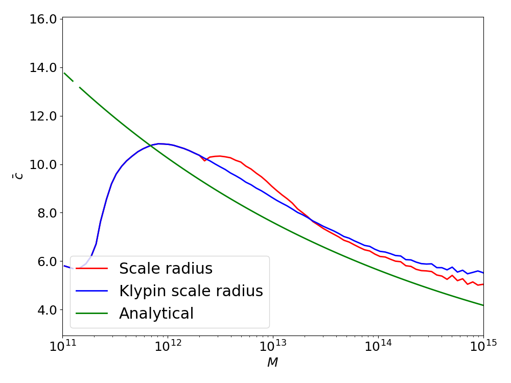
Figure II.1: Mean concentration of the benchmark ROCKSTAR halos as a function of their mass, calculated from both the scale radius and Klypin scale radius, as well as the analytical fit in (Cooray and Sheth, 2002) (Equation II.9).

To judge whether the NFW profile is a good choice for our purposes we first compared the benchmark mean concentration to the analytical fit in Equation II.9. ROCKSTAR fits an NFW profile by calculating both the scale radius $r_{s}$ and the Klypin scale radius $r_{s,K}$ (Klypin et al., 2011), which is derived from $v_{max}$, the maximum circular velocity, and $M_{vir}$. We have plotted the mean concentration computed from $r_{s}$ and $r_{s,K}$ against the analytical fit in Figure II.1. While the Klypin concentration demonstrates better numerical stability overall, it is not clear that it is more robust for halos with fewer than 100 particles as the authors of ROCKSTAR claim (Behroozi et al., 2013). We shall be using the Klypin concentration in all our methods discussed below. We note that while Equation II.9 seems to qualitatively capture the correct power law behaviour, the magnitude is too low by about 10-20%.

(a) $M=(0.62-2.2)\times 10^{13}h^{-1}\,M_{\odot}$

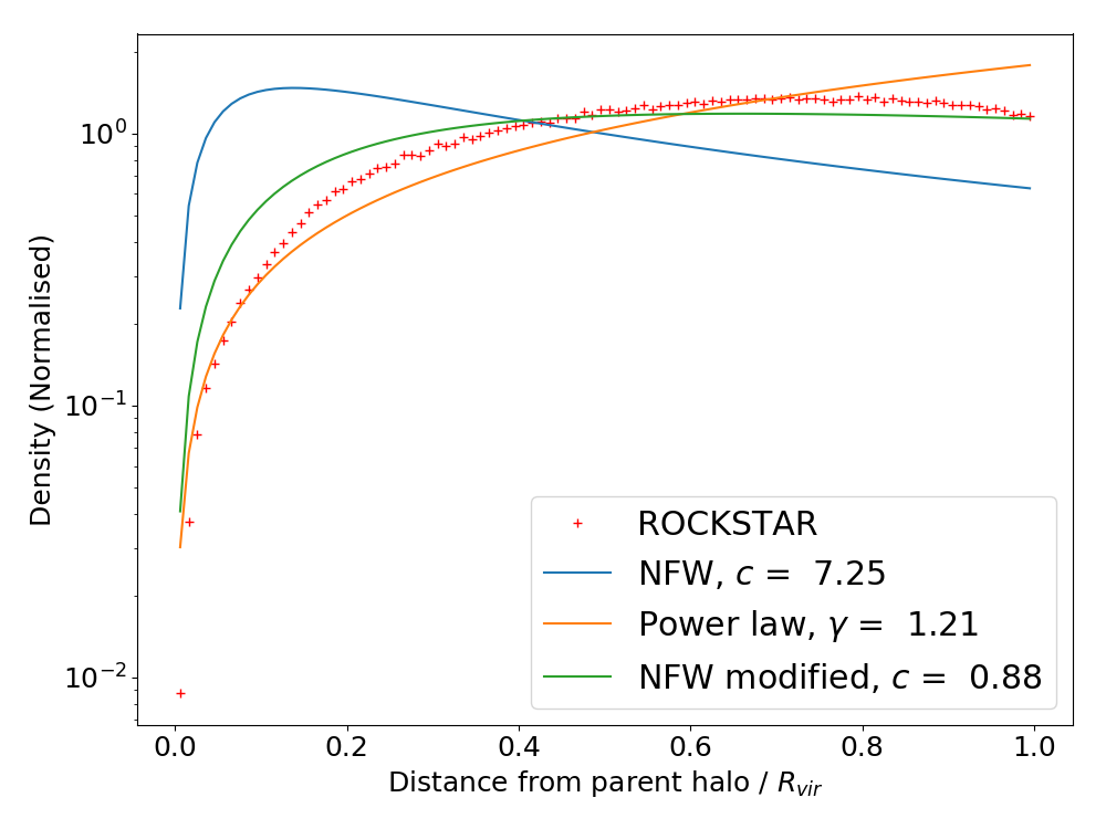
(b) $M=(2.2-7.6)\times 10^{13}h^{-1}\,M_{\odot}$

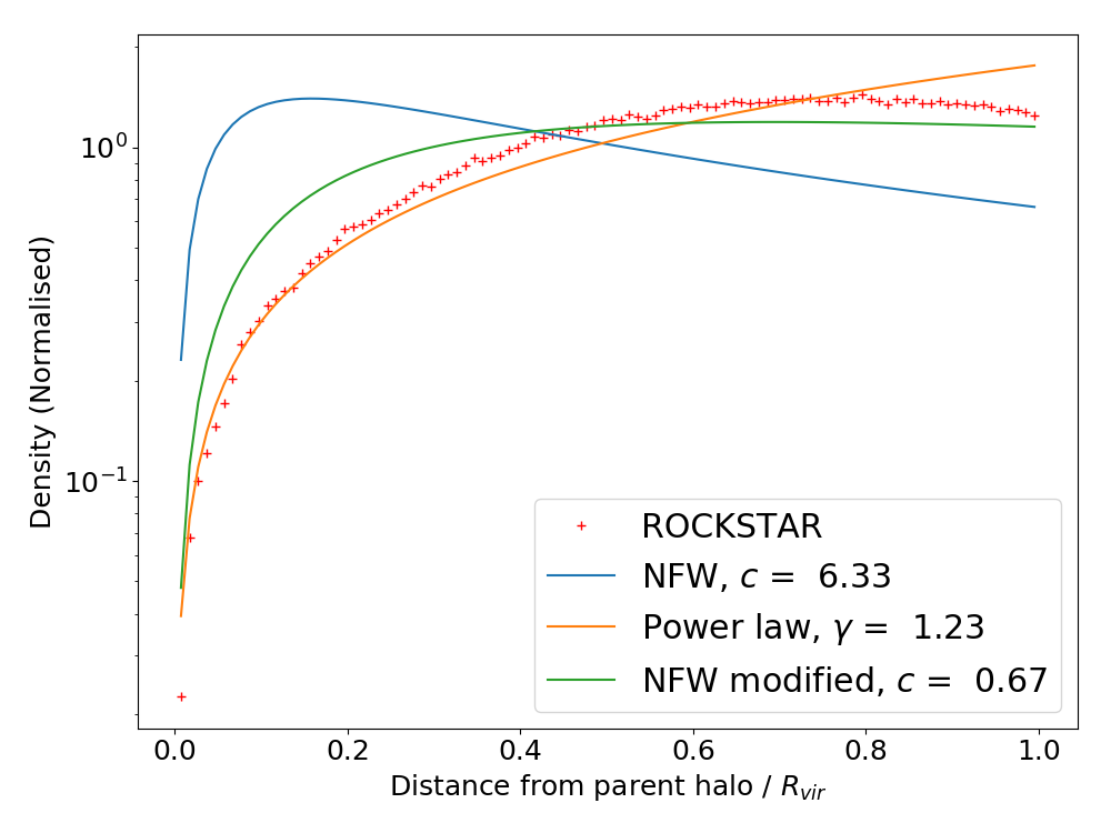
(c) $M=(0.76-2.7)\times 10^{14}h^{-1}\,M_{\odot}$

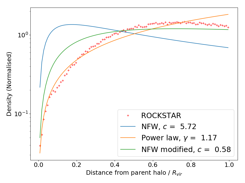
(d) $M=(2.7-9.3)\times 10^{14}h^{-1}\,M_{\odot}$

Figure II.2: The subhalo number density profile given by ROCKSTAR and NFW for parent halos in various mass bins, as well as a power law and modified NFW fits to the ROCKSTAR data. Distances are scaled by $R_{vir}$ measured by ROCKSTAR.

More importantly, while the NFW profile is used in the literature to populate halos with galaxies, it is ultimately a fit to the dark matter profile and may not reflect the subhalo density profile. Comparisons between the NFW profile and the number density profile for the ROCKSTAR benchmark catalogue at different mass bins is shown in Figure II.2. Throughout the paper we only populate subhalos to the virial radius $R_{vir}$. In these plots, the NFW profile is calculated using the average Klypin concentration given by ROCKSTAR for the mean halo mass of the bin. Additionally, distances are scaled by the virial radius $R_{vir}$, since that is the distance ROCKSTAR uses when fitting the NFW profile.

We found that the NFW profile is clearly more concentrated near the centre of the halo than the density profile of the benchmark subhalos (as observed already in, for example, (Jenkins et al., 2004; Libeskind et al., 2005; Moore et al., 2004; Gao et al., 2004)). Consequently, for a NFW profile based galaxy catalogue we expect a stronger correlation than the benchmark at small scales. We have also modified the NFW profile by keeping its functional form but changing the concentration, but this was not a good fit to the ROCKSTAR profile as shown in Figure II.2. Following (Frenk et al., 2016), we then adopted a universal power law $\rho\propto r^{-\gamma}$, where $\gamma\sim 1$ is our fiducial halo profile, such that

$$\text{CDF}_{\text{pow}}(r|M_{vir},c)=\left(\frac{r}{R_{vir}}\right)^{3-\gamma}.$$ (II.10)

We have found that $\gamma\approx 1$ is a satisfactory fit to the subhalo number distribution, as shown in Figures II.2 and II.3.

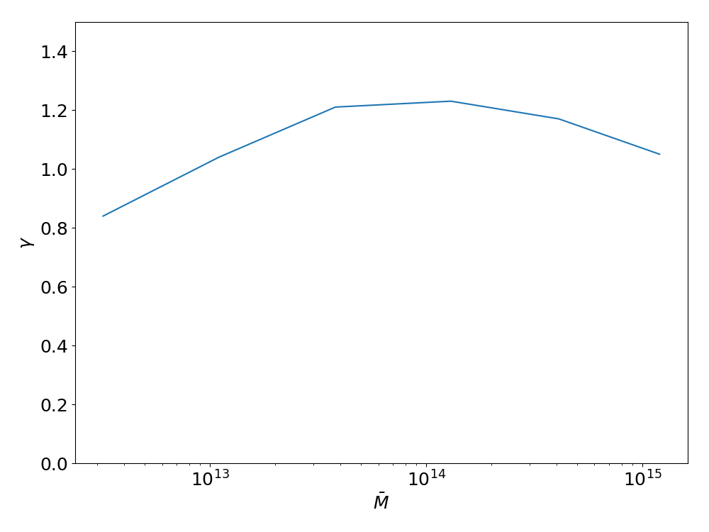
Figure II.3: Power law fit to the halo profile at different mass bins.

Halo Occupation Distribution (HOD)

Another important consideration in the population of parent halos is the halo occupation number, i.e. the number of galaxies per halo. A conventional way to phenomenologically model this is via a Halo Occupation Distribution (HOD) algorithm (Peacock and Smith, 2000; Scoccimarro et al., 2001; Berlind and Weinberg, 2002) which gives the mean occupation number as a function of the mass of the halo. A functional form for this algorithm consisting of 5 parameters is commonly used in the literature (Zheng et al., 2009; Eisenstein et al., 2017, 2018; Manera et al., 2013):

$$\bar{N}_{\text{cent}}(M) =\frac{1}{2}\operatorname{erfc}\left[-\frac{\ln M/M_{0}}{\sqrt{2}\sigma}\right],$$ (II.11)

$$\bar{N}_{\text{sat}}(M) =\left(\frac{M-\kappa M_{0}}{M_{1}}\right)^{\alpha},$$ (II.12)

where $\bar{N}_{\text{cent}}$ is the expected number of central galaxies and $\bar{N}_{\text{sat}}$ the expected number of satellite galaxies such that $\bar{N}_{g}(M)=\bar{N}_{\text{cent}}(M)+\bar{N}_{\text{sat}}(M)$. Here $M_{0}$ denotes the typical minimum mass scale for a halo to have a central galaxy, and $\sigma$ is the parameter that controls the scatter around that mass. $\kappa M_{0}$ sets the cutoff scale for a halo to host a satellite, $M_{1}$ is the typical additional mass above $\kappa M_{0}$ for a halo to have one satellite galaxy, and $\alpha$ is the exponent that controls the tail of the HOD, and therefore has a strong influence on the number of high-mass halos.

Instead of using the error function we employ a Heaviside cut for $\bar{N}_{\text{cent}}$:

$$\bar{N}_{\text{cent}}(M)=\theta(M-M_{0}),$$ (II.13)

reducing the number of parameters to 4. This is appropriate as we impose a mass cut on the parent halo when constructing the benchmark galaxy catalogue. These 4 parameters give us freedom to tweak the power spectrum and bispectrum of our galaxy mock catalogues to better reproduce those of the benchmark sample. The total number of galaxies is

$$n_{g}=\int dM\,n(M)\left(\theta(M-M_{0})+\left(\frac{M-\kappa M_{0}}{M_{1}}\right)^{\alpha}\right),$$ (II.14)

where $n(M)$ is the halo mass function that gives the number density of halos for a given mass $M$. If the variation in the parameters are small we obtain the following perturbation to the number of galaxies to first order:

$$\Delta n_{g}$$

$$={} -\int dM\,n(M)$$

$$\times\Bigg{(}\frac{\Delta M_{0}}{M_{0}}M_{0}\left(\delta(M-M_{0})+\frac{\alpha\kappa}{M_{1}}\left(\frac{M-\kappa M_{0}}{M_{1}}\right)^{\alpha-1}\right)$$

$$\qquad+\frac{\Delta\kappa}{\kappa}\kappa\frac{\alpha M_{0}}{M_{1}}\left(\frac{M-\kappa M_{0}}{M_{1}}\right)^{\alpha-1}$$

$$\qquad+\frac{\Delta M_{1}}{M_{1}}M_{1}\frac{\alpha(M-\kappa M_{0})}{M^{2}_{1}}\left(\frac{M-\kappa M_{0}}{M_{1}}\right)^{\alpha-1}$$

$$\qquad-\frac{\Delta\alpha}{\alpha}\alpha\log\left(\frac{M-\kappa M_{0}}{M_{1}}\right)\left(\frac{M-\kappa M_{0}}{M_{1}}\right)^{\alpha}\Bigg{)},$$ (II.15)

and we enforce $\Delta n_{g}=0$ to conserve particle number when changing the parameters.

In Figure II.4 we show the HOD $\bar{N}_{g}(M)$ from our benchmark ROCKSTAR catalogue (which will be referred to as the benchmark HOD model below), and the best fit for the 4-parameter HOD while keeping the total number of galaxies constant. As a comparison we also obtain an unconstrained fit to the benchmark HOD. The best fit parameters for the constrained fit are $\log(M_{0})=11.76$, $\kappa=0.89$,$\log(M_{1})=13.35$ and $\alpha=1.04$, with only a $4\times 10^{-4}\%$ deficiency in the number of galaxies.

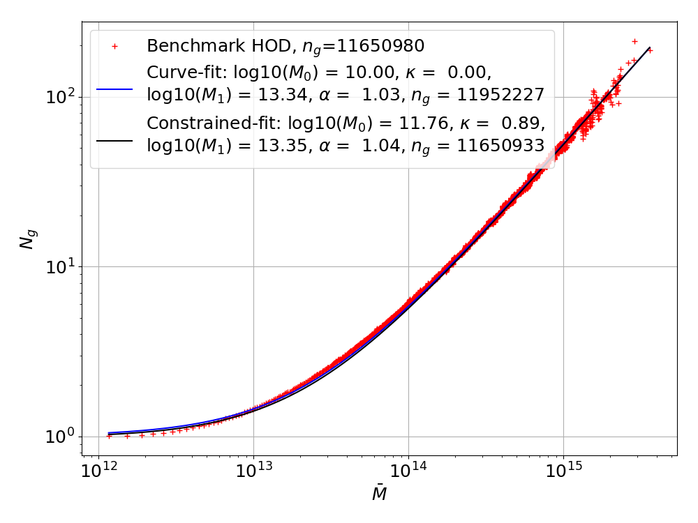
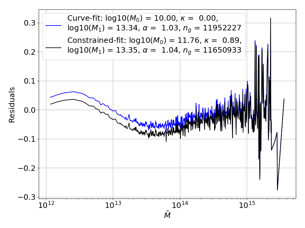
Figure II.4: Left panel: Fits to the benchmark HOD with our 4 parameters, both constraining and not constraining the total number of galaxies. Right panel: Residuals of these fits.

Halo polyspectra

Power spectrum and Bispectrum

The leading source of cosmological information, and hence the principal diagnostic of our methods, is the two-point correlator, or power spectrum $P(k)$ of an overdensity field $\delta(\mathbf{x})$:

$$\expectationvalue{\delta(\mathbf{k})\delta(\mathbf{k}^{\prime})}=(2\pi)^{3}\delta_{D}(\mathbf{k}+\mathbf{k}^{\prime})P(k),$$ (III.1)

where $\delta_{D}$ is the Dirac delta function. The power spectra of our benchmark dark matter and galaxy catalogues at redshifts $z=0,0.5,1$ are plotted in Figure III.1. Our galaxy catalogue consists of parent halos with mass in the range of $1\times 10^{12}$ and $3.2\times 10^{15}h^{-1}\,M_{\odot}$ and all their subhalos, and has a number density of $0.0056\,h^{3}\,\text{Mpc}^{-3}$, which is similar to the number density of the LOWZ galaxy sample in BOSS at low redshift (Anderson et al., 2014). It is well known in the literature that while the dark matter power spectrum grows with time, the growth of the halo power spectrum is slow (Gottlöber et al., 1999; Kravtsov and Klypin, 1999). At large scales the linear bias relationship $b_{1}=\delta_{g}/\delta$ between dark matter and galaxies tends to a constant (Mann et al., 1998), and since the dark matter power spectrum grows as $D^{2}_{1}(z)$ at these scales, where $D_{1}(z)$ is the linear growth factor, we expect $b_{1}(z)\propto 1/D_{1}(z)$. This is also shown clearly in Figure III.1, giving a value of $b_{1}\approx 1.1$.

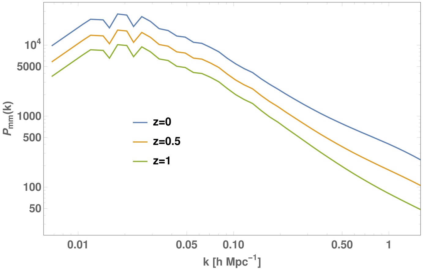
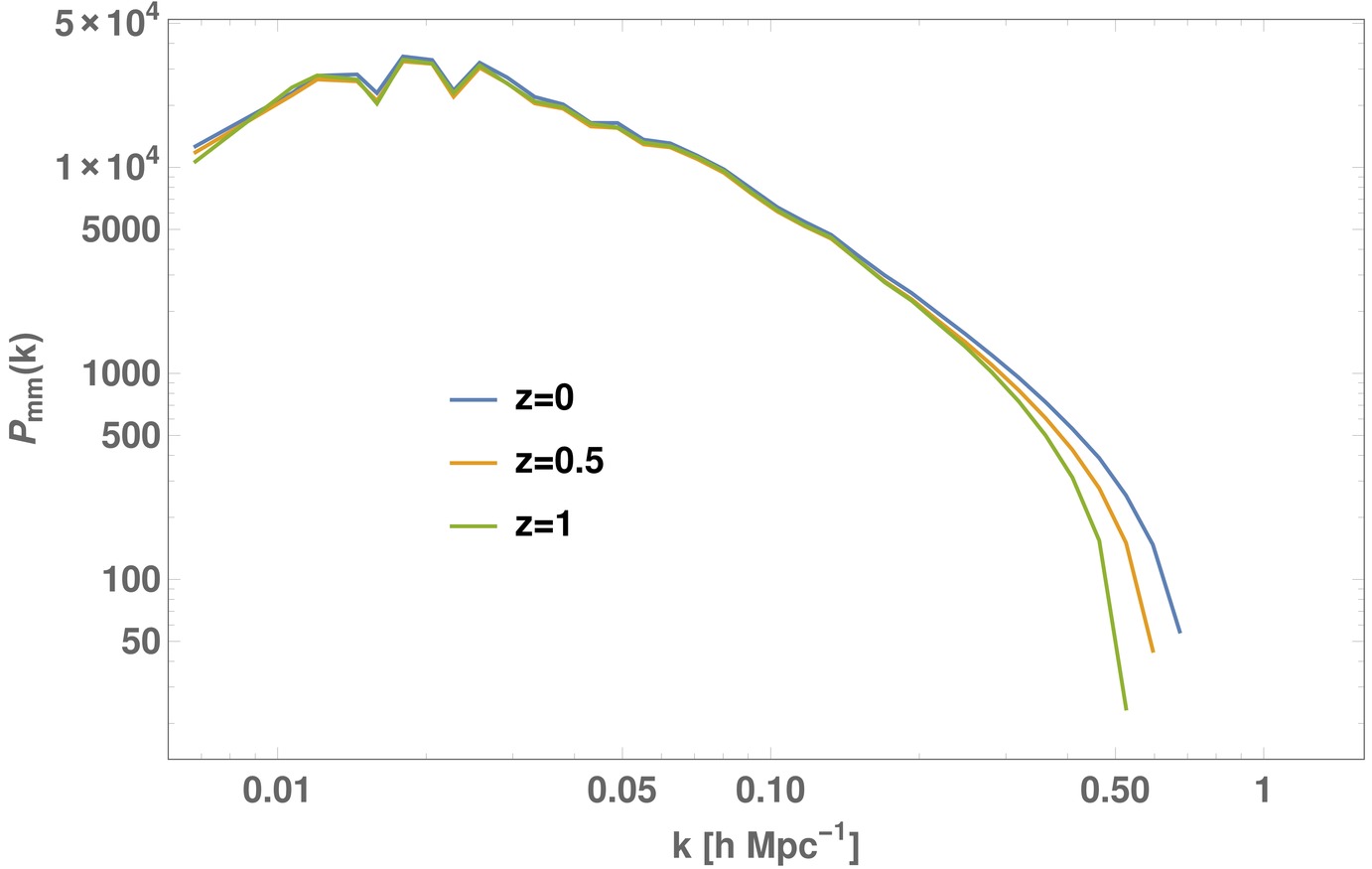
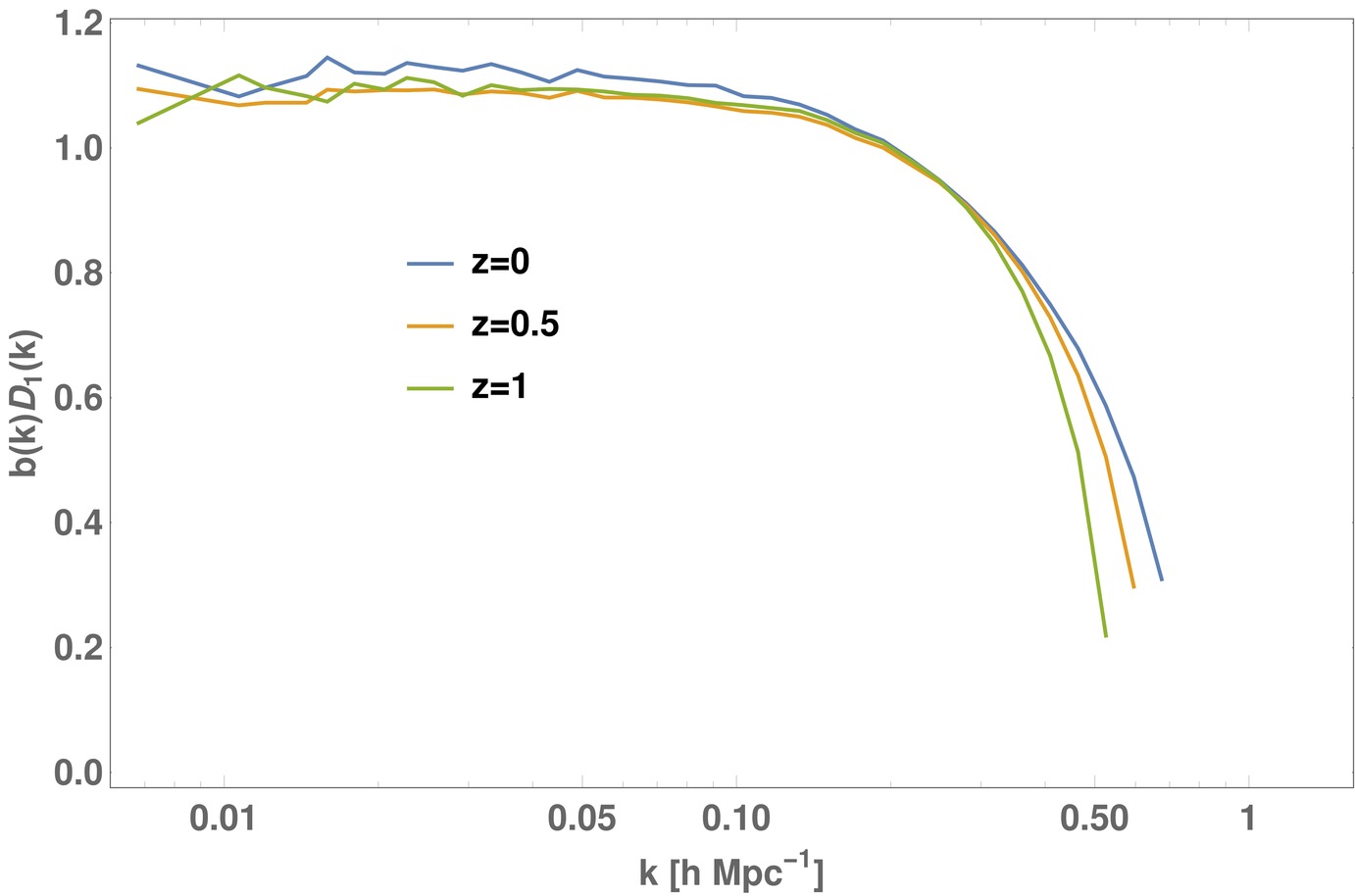
Figure III.1: Redshift evolution of the estimated power spectrum of the $1280\,h^{-1}$ Mpc benchmark GADGET-3 dark matter simulation (top left), and the benchmark galaxy mock catalogue derived from it using ROCKSTAR (after shot noise subtraction, top right), plotted up to $k_{max}=1.6\,h\,\text{Mpc}^{-1}$. The bottom panel shows the product between the bias parameter, obtained from $b=\sqrt{P_{hh}/P_{mm}}$, and the linear growth factor $D_{1}$, which tends to a constant at large scales irrespective of redshift.

For mildly non-linear scales the primary diagnostic is the three point correlation function or bispectrum $B_{\delta}(k_{1},k_{2},k_{3})$:

$$\expectationvalue{\delta(\mathbf{k}_{1})\delta(\mathbf{k}_{2})\delta(\mathbf{k}_{3})}$$

$$\qquad=(2\pi)^{3}\delta_{D}(\mathbf{k}_{1}+\mathbf{k}_{2}+\mathbf{k}_{3})B_{\delta}(k_{1},k_{2},k_{3}).$$ (III.2)

Due to statistical isotropy and homogeneity, in configuration space the bispectrum only depends on the wavenumbers $k_{i}$ in the absence of redshift space distortions. Additionally the delta function, arising from momentum conservation, imposes the triangle condition on the wavevectors so the three $k_{i}$ when taken as lengths must be able to form a triangle. Together with a parameter $k_{max}$ which defines the resolution of the data, the bispectrum occupies a tetrapydal domain $\mathcal{V}_{B}$ in $k$-space, as shown in the left panel of Figure III.2. We have found it useful to split it in half to make apparent its internal morphology as illustrated in the right panel of Figure III.2. The bispectra plots in this paper are generated with ParaView (Ahrens et al., 2005), an open source scientific visualisation tool.

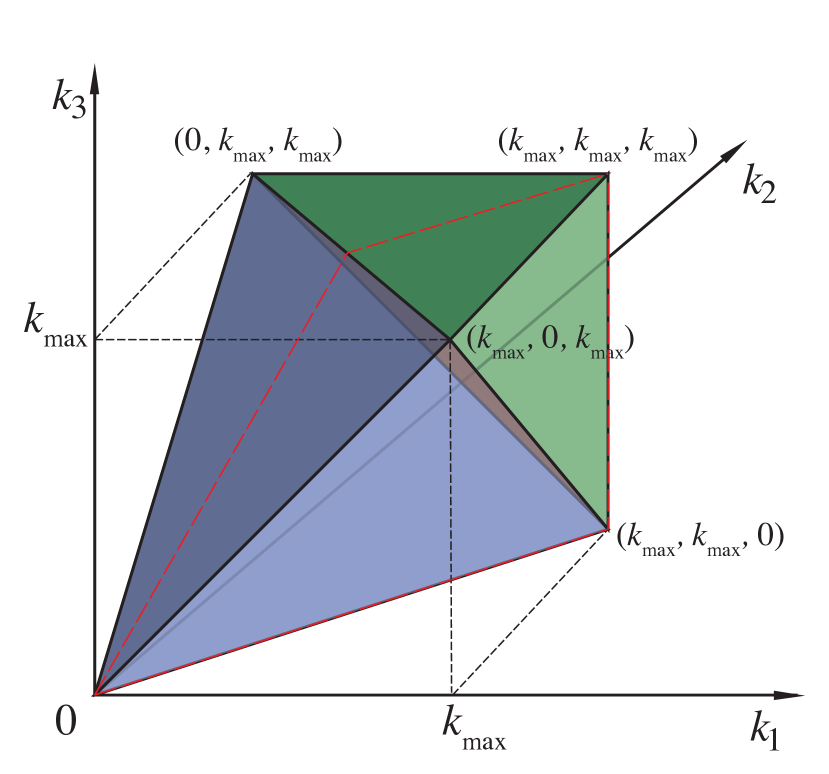
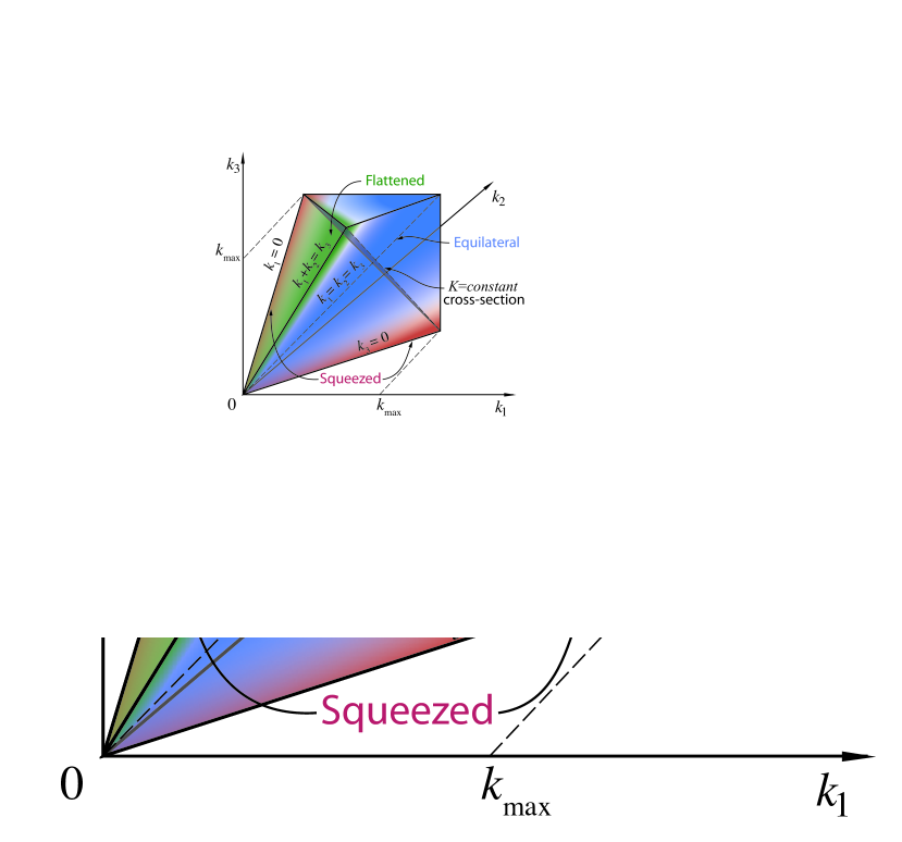
Figure III.2: Left panel: The full tetrapyd bispectrum domain $\mathcal{V}_{B}$ consists of a tetrahedral region (blue) defined by the wavevector triangle condition $\mathbf{k}_{1}+\mathbf{k}_{2}+\mathbf{k}_{3}=0$, together with a pyramidal region (green) bounded by the resolution limit $k_{\text{max}}$. Right panel: To show the internal structure of the tetrapyd we split it along the red dashed line, showing only the back half with $k_{1}<k_{2}$. Colour-coded regions show the location of the ‘squeezed’ (red), ‘flattened’ (green) and ‘equilateral’ or ‘constant’ (blue) shape signals. The scale dependence of the bispectrum is reflected by the $K\equiv k_{1}+k_{2}+k_{3}=\text{const.}$ cross sectional planes (Lazanu et al., 2016).

Due to the large number of triangle configurations, numerical estimation of the full bispectrum is computationally expensive. In this paper we use the newly rewritten MODAL-LSS method for the efficient and accurate estimation of the bispectrum for any overdensity field $\delta$ (Hung et al., 2019). The full bispectra of the benchmark catalogue at various redshifts thus obtained are shown in Figure III.3, along with the corresponding dark matter bispectra plotted for reference.

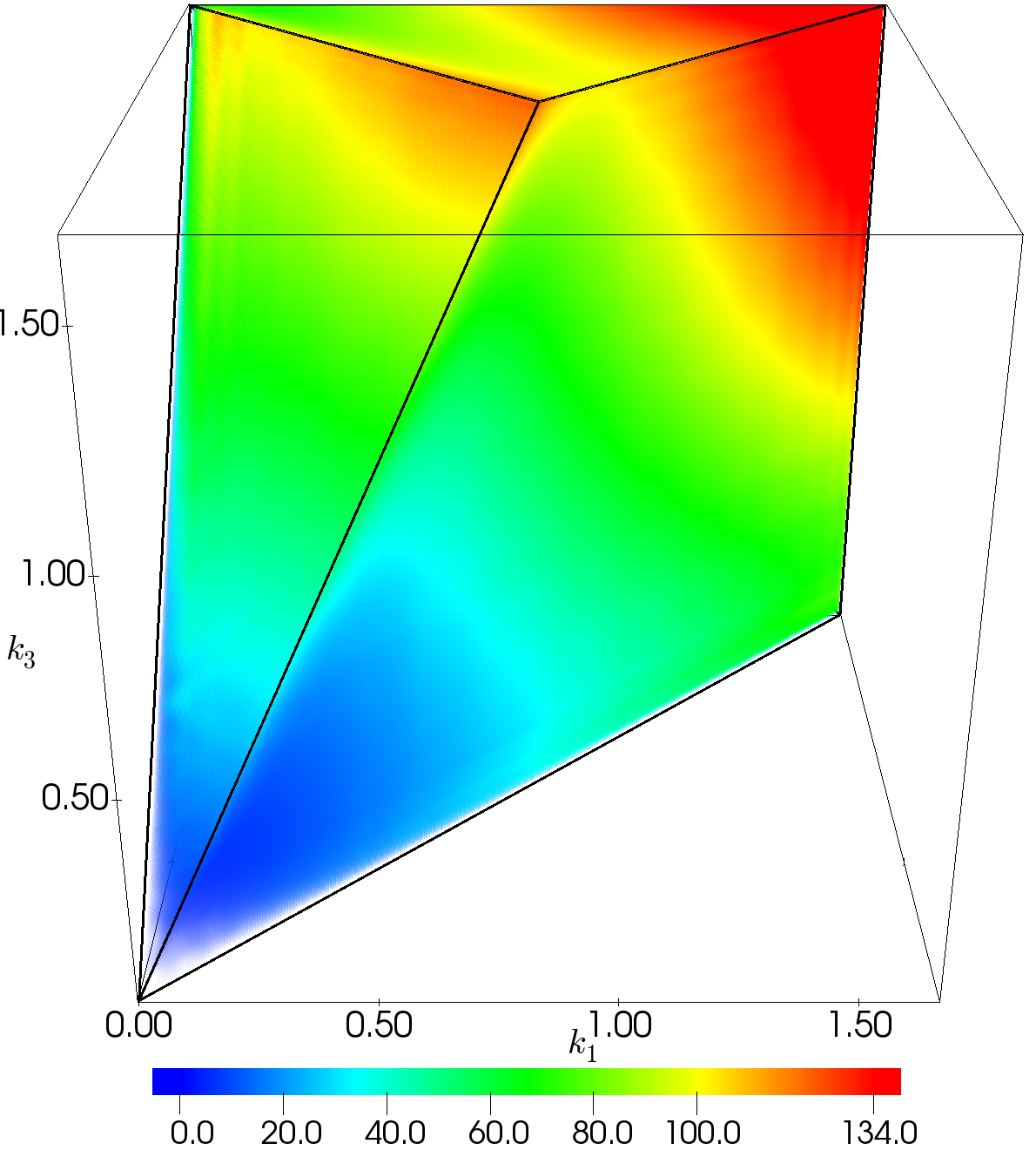
(a) Dark matter, $z=1$

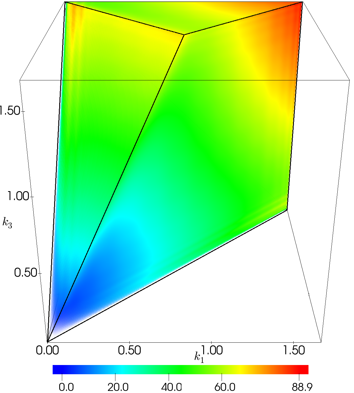
(b) Galaxies, $z=1$

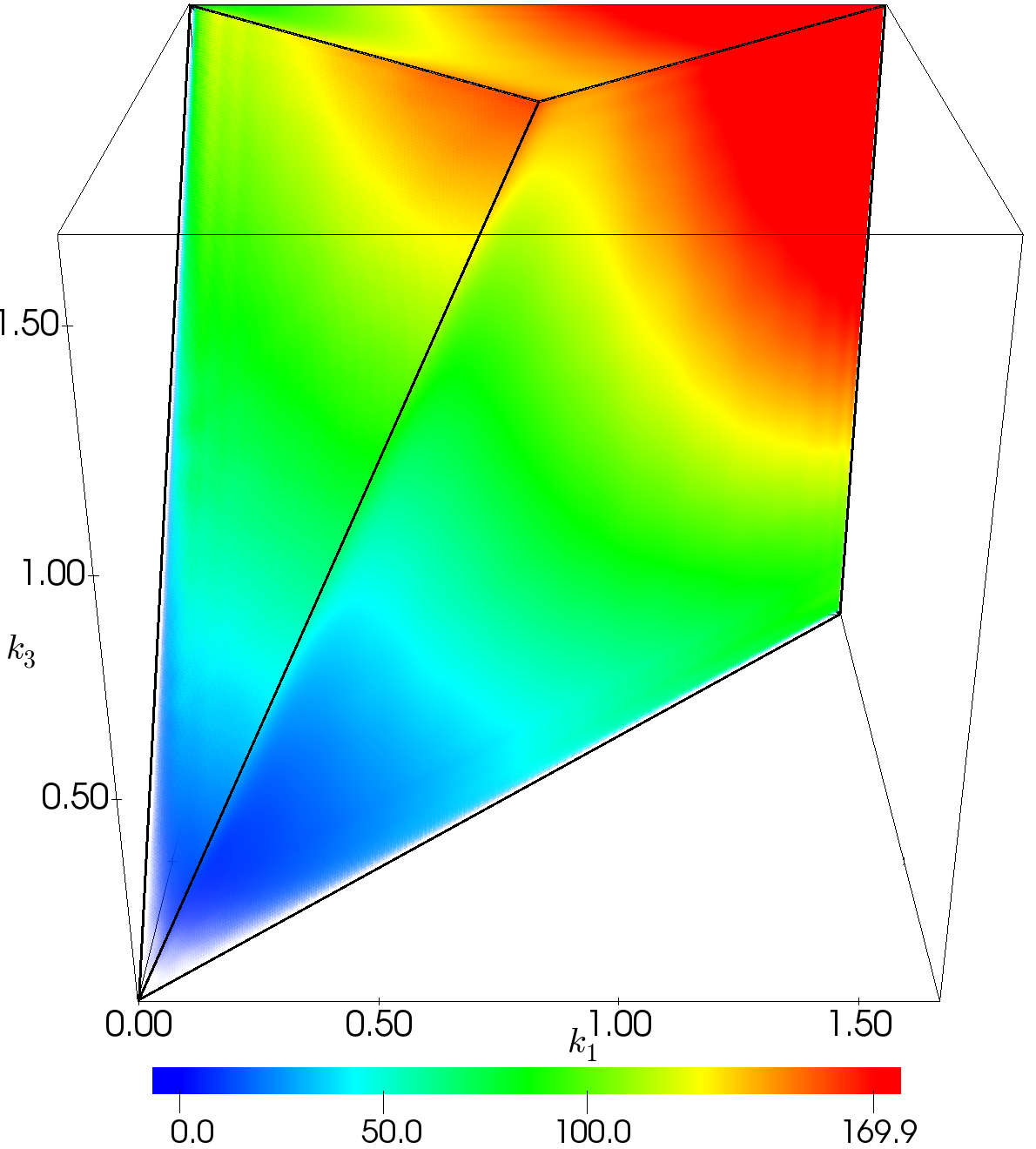
(c) Dark matter, $z=0.5$

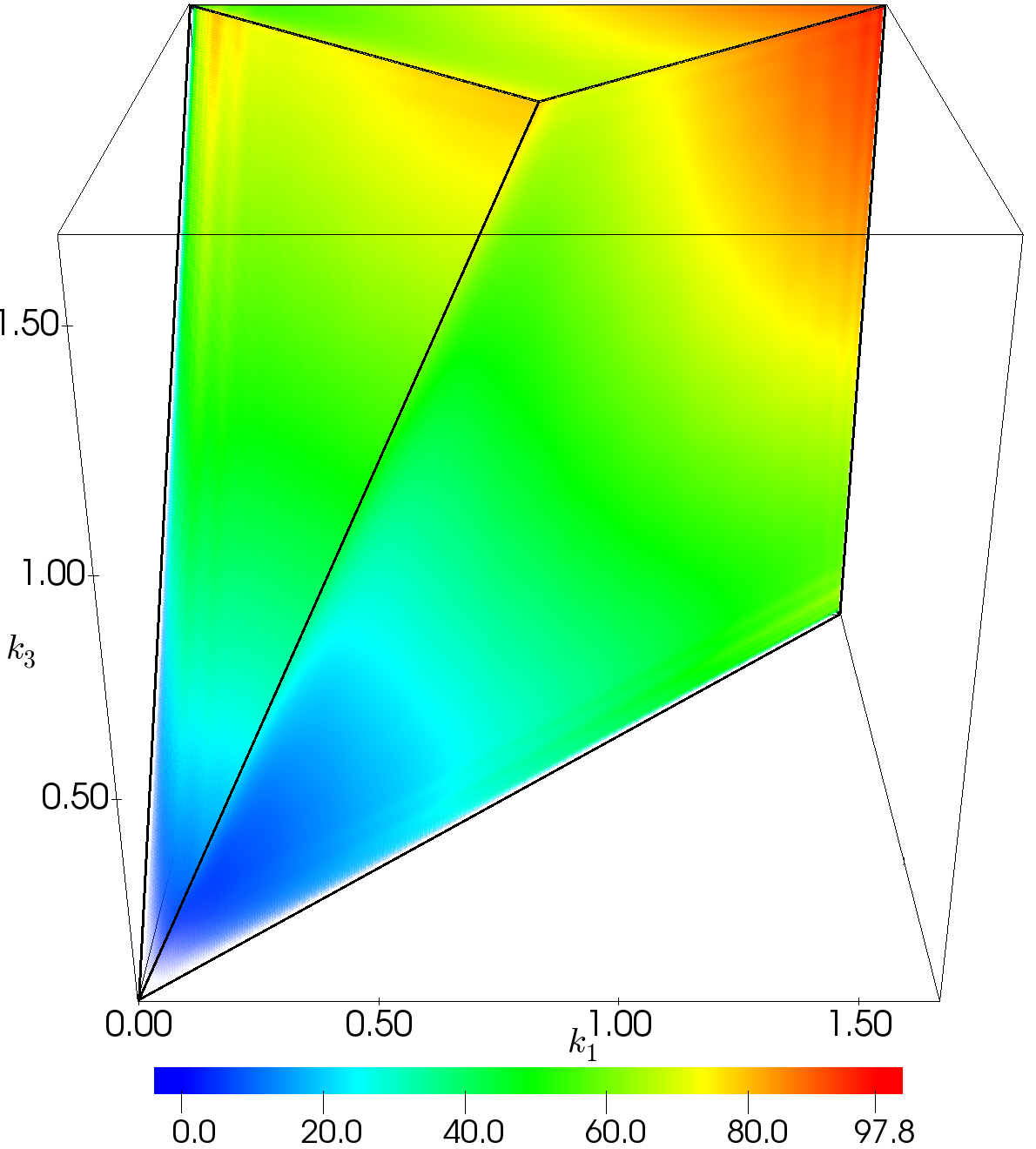
(d) Galaxies, $z=0.5$

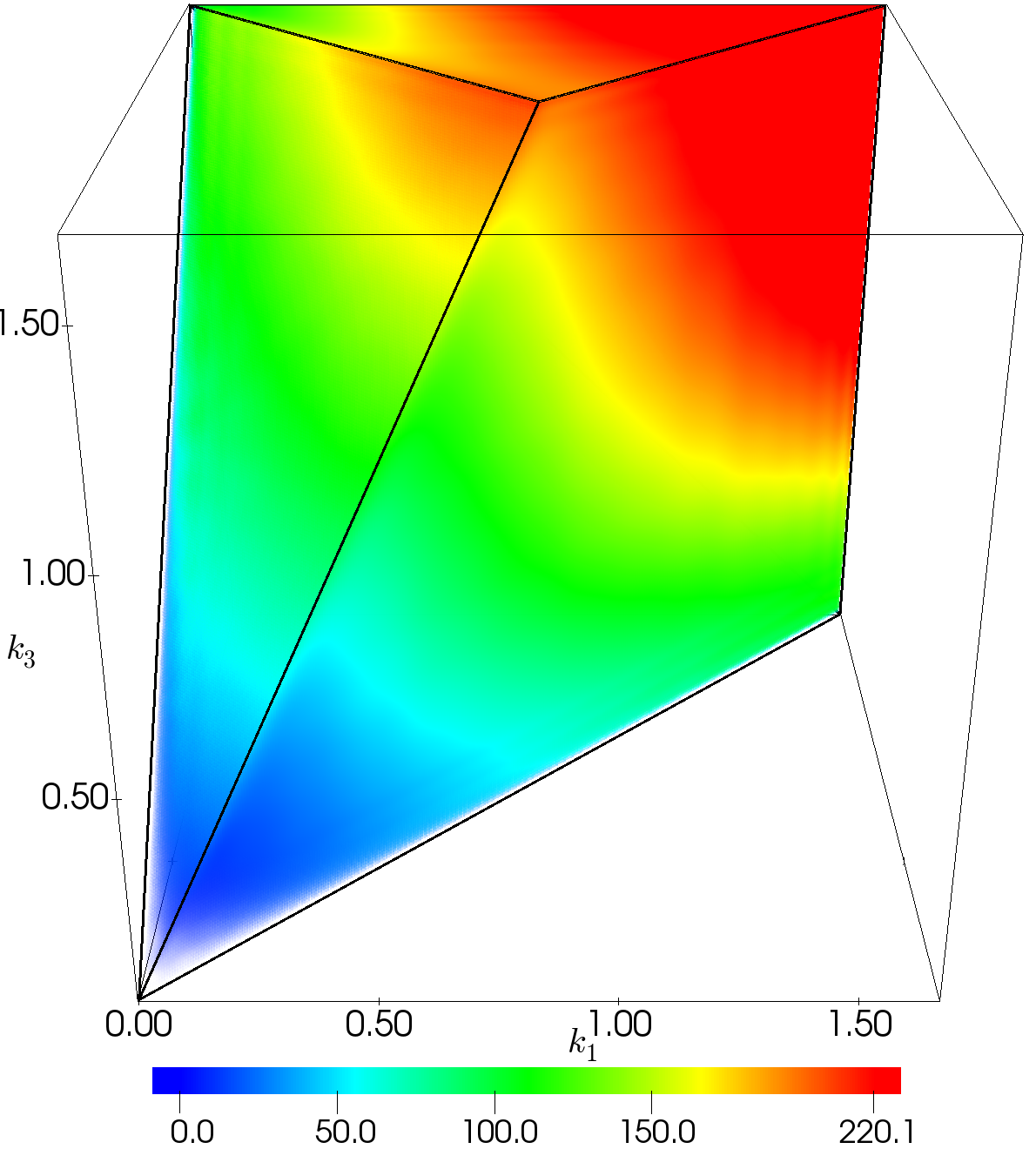
(e) Dark matter, $z=0$

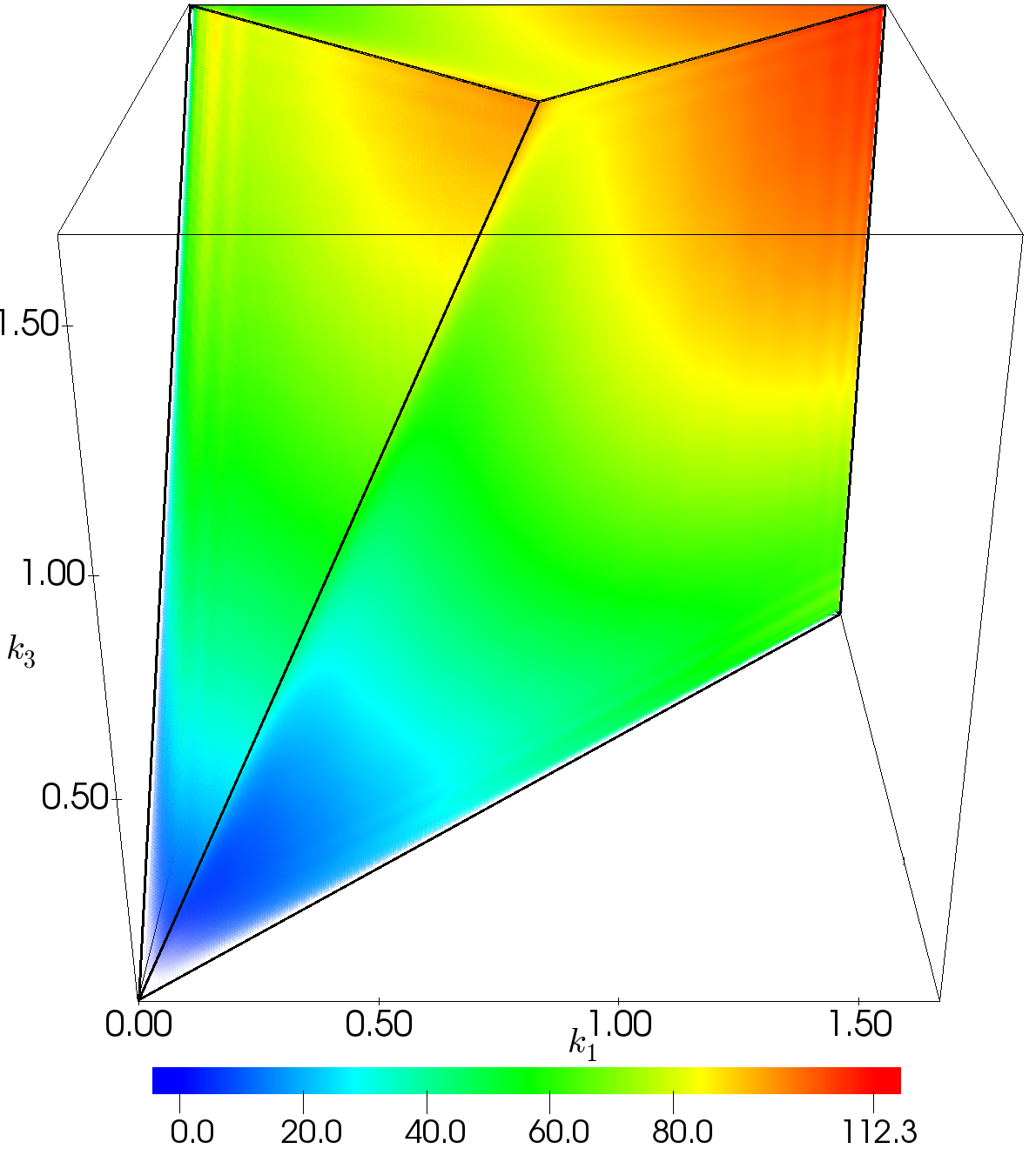
(f) Galaxies, $z=0$

Figure III.3: Redshift evolution of the estimated bispectra of the $1280\,h^{-1}$ Mpc benchmark GADGET-3 dark matter simulation, and the benchmark galaxy mock catalogue derived from it using ROCKSTAR, plotted up to $k_{max}=1.6\,h\,\text{Mpc}^{-1}$.

MODAL-LSS bispectrum methodology

Here we give a brief summary of the MODAL-LSS algorithm. We first approximate the signal-to-noise weighted estimated bispectrum of a density field, $\sqrt{\frac{k_{1}k_{2}k_{3}}{P(k_{1})P(k_{2})P(k_{3})}}\hat{B}_{\delta}(k_{1},k_{2},k_{3})$, by expanding it in a general separable basis:

$$\sqrt{\frac{k_{1}k_{2}k_{3}}{P(k_{1})P(k_{2})P(k_{3})}}\hat{B}_{\delta}(k_{1},k_{2},k_{3})$$

$$\quad\approx\sum_{mn}^{n_{max}}\gamma^{-1}_{nm}\beta^{Q}_{m}Q^{\texttt{MODAL-LSS}{}}_{n}(k_{1}/k_{max},k_{2}/k_{max},k_{3}/k_{max}),$$ (III.3)

where $P(k)$ is the power spectrum of the density field. The information in the full bispectrum is compressed into these $\mathcal{O}(1000)$ $\beta^{Q}_{m}$ coefficients, and it has been shown to be superior to other bispectrum estimators in terms of data compression (Seery et al., 2017). The basis functions $Q^{\texttt{MODAL-LSS}{}}_{n}$ are symmetrised products over one dimensional functions $q_{r}$:

$$Q^{\texttt{MODAL-LSS}{}}_{n}(x,y,z)\equiv q_{\{r}(x)q_{s}(y)q_{t\}}(z),$$ (III.4)

with $\{\dots\}$ representing symmetrisation over the indices $r,s,t$, and each $n$ corresponds to a combination of $r,s,t$. The relationship between $n$ and $r,s,t$ is ‘slice ordering’ which orders the triples by the sum $r+s+t$. $k_{max}$ is the resolution of the tetrahedral domain defined above. $\gamma_{nm}$ is the inner product between $Q^{\texttt{MODAL-LSS}{}}_{n}$ functions over the tetrapyd domain:

$$\gamma_{nm}\equiv\frac{V}{\pi}\int_{\mathcal{V}_{B}}dV_{k}Q_{n}Q_{m},$$ (III.5)

where $V=(2\pi)^{3}\delta_{D}(\mathbf{0})$ is the volume of the simulation box. There is a freedom in the choice of $q_{r}$, provided the $Q^{\texttt{MODAL-LSS}{}}_{n}$ basis is orthogonal, or can be made orthogonal. We employ shifted Legendre polynomials $\tilde{P}_{l}(x)=P_{l}(2x-1)$, such that $\tilde{P}_{l}(x)$ is orthogonal over the interval $\left[0,1\right]$ instead of the usual $\left[-1,1\right]$ for $P_{l}(x)$.

For $\hat{B}_{\delta}(k_{1},k_{2},k_{3})=\frac{1}{V}\delta(\mathbf{k}_{1})\delta(\mathbf{k}_{2})\delta(\mathbf{k}_{3})$ we multiply both sides of Equation III.3 by $Q^{\texttt{MODAL-LSS}{}}_{m}(k_{1}/k_{max},k_{2}/k_{max},k_{3}/k_{max})$ and integrate over $\mathcal{V}_{B}$ to find

$$\beta^{Q}_{n} =\frac{1}{\pi}\int_{\mathcal{V}_{B}}dV_{k}\sqrt{\frac{k_{1}k_{2}k_{3}}{P(k_{1})P(k_{2})P(k_{3})}}\delta_{\mathbf{k}_{1}}\delta_{\mathbf{k}_{2}}\delta_{\mathbf{k}_{3}}$$

$$\qquad\qquad\qquad\times q_{\{r}(\frac{k_{1}}{k_{max}})q_{s}(\frac{k_{2}}{k_{max}})q_{t\}}(\frac{k_{3}}{k_{max}})$$

$$=\int_{\mathbf{k}_{1},\mathbf{k}_{2},\mathbf{k}_{3}}(2\pi)^{6}\delta_{D}(\mathbf{k}_{1}+\mathbf{k}_{2}+\mathbf{k}_{3})$$

$$\qquad\qquad\qquad\times\frac{\delta_{\mathbf{k}_{1}}\delta_{\mathbf{k}_{2}}\delta_{\mathbf{k}_{3}}}{\sqrt{k_{1}P(k_{1})k_{2}P(k_{2})k_{3}P(k_{3})}}$$

$$\qquad\qquad\qquad\times q_{\{r}(\frac{k_{1}}{k_{max}})q_{s}(\frac{k_{2}}{k_{max}})q_{t\}}(\frac{k_{3}}{k_{max}})$$

$$=(2\pi)^{3}\int d^{3}x\int\frac{\prod_{i}d^{3}k_{i}}{(2\pi)^{9}}e^{i(\mathbf{k}_{1}+\mathbf{k}_{2}+\mathbf{k}_{3})\cdot\mathbf{x}}$$

$$\qquad\qquad\qquad\times\frac{\delta_{\mathbf{k}_{1}}\delta_{\mathbf{k}_{2}}\delta_{\mathbf{k}_{3}}}{\sqrt{k_{1}P(k_{1})k_{2}P(k_{2})k_{3}P(k_{3})}}$$

$$\qquad\qquad\qquad\times q_{\{r}(\frac{k_{1}}{k_{max}})q_{s}(\frac{k_{2}}{k_{max}})q_{t\}}(\frac{k_{3}}{k_{max}})$$

$$=(2\pi)^{3}\int d^{3}x\,M_{r}(\mathbf{x})M_{s}(\mathbf{x})M_{t}(\mathbf{x}),$$ (III.6)

where we define

$$M_{r}(\mathbf{x})\equiv\int\frac{d^{3}k}{(2\pi)^{3}}\frac{\delta_{\mathbf{k}}q_{r}(k/k_{max})}{\sqrt{kP(k)}}e^{i\mathbf{k}\cdot\mathbf{x}},$$ (III.7)

which is an inverse Fourier transform, and $\int_{\mathbf{k}_{1},\mathbf{k}_{2},\mathbf{k}_{3}}=\int\frac{d^{3}k_{1}}{(2\pi)^{3}}\frac{d^{3}k_{2}}{(2\pi)^{3}}\frac{d^{3}k_{3}}{(2\pi)^{3}}$. In the second line we used the identity

$$\int\frac{d^{3}k_{1}}{(2\pi)^{3}}\frac{d^{3}k_{2}}{(2\pi)^{3}}\frac{d^{3}k_{3}}{(2\pi)^{3}}(2\pi)^{6}\delta^{2}_{D}\left(\mathbf{k}_{1}+\mathbf{k}_{2}+\mathbf{k}_{3}\right)F$$

$$\quad=\frac{V}{8\pi^{4}}\int_{\mathcal{V}_{B}}dk_{1}dk_{2}dk_{3}\,k_{1}k_{2}k_{3}F.$$ (III.8)

In summary, we have reduced the 9-dimensional integrals involved in bispectrum estimation to a number of (inverse) Fourier transforms which can be evaluated efficiently with the fast Fourier transform (FFT) algorithm, together with an integral over the spatial extent of the data set (Section III.2) which can highly parallelised. Additionally we have compressed the full 3D bispectral information to $\mathcal{O}(1000)$ $\beta^{Q}_{n}$ coefficients, which are much easier to manipulate.

To make comparisons between bispectra $B_{i}$ and $B_{j}$ we first define inner products between them as

$$\left[B_{i},B_{j}\right]\equiv\frac{V}{\pi}\int_{\mathcal{V}_{B}}dV_{k}\,k_{1}k_{2}k_{3}\frac{B_{i}(k_{1},k_{2},k_{3})B_{j}(k_{1},k_{2},k_{3})}{P(k_{1})P(k_{2})P(k_{3})}.$$ (III.9)

We define two correlators between bispectra. The first is the total correlator $\mathcal{T}$:

$$\mathcal{T}(B_{i},B_{j}) \equiv 1-\sqrt{\frac{\left[B_{j}-B_{i},B_{j}-B_{i}\right]}{\left[B_{j},B_{j}\right]}},$$ (III.10)

which is a stringent test of correlation between bispectra, but is susceptible to degradation by statistical noise. The other one is the $f_{nl}$ correlator, named as such due to its similarity to the optimal $\langle\hat{f}_{nl}\rangle$ estimator for the amplitude of a theoretical shape (see (Hung et al., 2019)), as:

$$f_{nl}(B_{i},B_{j})\equiv\frac{\big{[}B_{i},B_{j}\big{]}}{\big{[}B_{j},B_{j}\big{]}}.$$ (III.11)

The $f_{nl}$ correlator can be thought of as proportional to the cosine between the two shapes, weighted by the magnitude of $B_{j}$. This correlator is therefore appropriate for the compression of 3D bispectral information into a one-dimensional function of $k_{max}$.

We further define a ‘sliced’ correlator between bispectra which integrates over transverse degrees of freedom $K\equiv k_{1}+k_{2}+k_{3}=\text{const.}$ on the tetrahedron:

$$\left[B_{i},B_{j}\right]^{S}_{K}\equiv\frac{V}{\pi}\int_{\Delta\mathcal{V}_{B}}dV_{k}\,k_{1}k_{2}k_{3}\frac{B_{i}(k_{1},k_{2},k_{3})B_{j}(k_{1},k_{2},k_{3})}{P(k_{1})P(k_{2})P(k_{3})}.$$ (III.12)

The new restricted integration region, $\Delta\mathcal{V}_{B}$, encompasses a range of these $K$ slices such that:

$$K<k_{1}+k_{2}+k_{3}<K+\Delta K.$$ (III.13)

Similarly we define the sliced $f_{nl}$ correlator as

$$f^{S}_{nl}(B_{i},B_{j},K)\equiv\frac{\big{[}B_{i},B_{j}\big{]}^{S}_{K}}{\big{[}B_{j},B_{j}\big{]}^{S}_{K}}.$$ (III.14)

Halo three-shape model

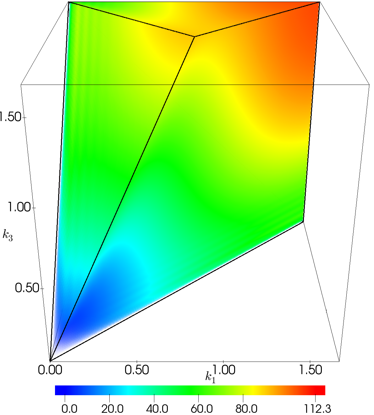
Figure III.4: Best fit three-shape model to the bispectrum of the benchmark ROCKSTAR catalogue.

Figure III.5: Sliced $f_{nl}$ correlation between the best fit three-shape model to the benchmark, and the benchmark. The feature observed at $K/3=1.1\,h\,\text{Mpc}^{-1}$ here is due to the transition from the tetrahedral region in the bottom to the pyramid at the top, causing a kink in the sliced correlator, and is not a real physical effect.

The three-shape model was proposed in (Lazanu et al., 2016, 2017) as a phenomenological model to quantitatively describe the dark matter bispectrum $B_{\rm mmm}(k_{1},k_{2},k_{3})$, consisting of a linear combination of the ‘constant’ one-halo model on small length scales, the tree-level gravitational bispectrum on the largest, and a local or ‘squeezed’ shape interpolating on intermediate scales. The combined three-shape model takes the following form:

$$B_{\text{3-shape}}(k_{1},k_{2},k_{3})$$

$$=\sum^{3}_{i=1}f_{i}(K)B^{i}(k_{1},k_{2},k_{3})$$

$$=f_{1h}(K)B^{\text{const}}(k_{1},k_{2},k_{3})+f_{2h}(K)B^{\text{squeez}}(k_{1},k_{2},k_{3})$$

$$\quad+f_{3h}(K)B^{\text{treeNL}}(k_{1},k_{2},k_{3}),$$ (III.15)

where the $f_{i}(K)$ are scale-dependent amplitudes and the constant, squeezed and tree-level shapes are respectively:

$$B^{\text{const}}(k_{1},k_{2},k_{3})=1,$$ (III.16)

$$B^{\text{squeez}}(k_{1},k_{2},k_{3})=\frac{1}{3}[P_{\text{lin}}(k_{1})P_{\text{lin}}(k_{2})$$

$$\qquad\qquad+2\,\text{perms.},$$ (III.17)

$$B^{\text{treeNL}}(k_{1},k_{2},k_{3})=2P_{\text{NL}}(k_{1})P_{\text{NL}}(k_{2})F^{(s),\Lambda}_{2}(\mathbf{k}_{1},\mathbf{k}_{2})$$

$$\qquad\qquad+2\,\text{perms.}.$$ (III.18)

Here, $P_{\text{lin}}$ denotes the linear dark matter power spectrum, $P_{\text{NL}}$ is the non-linear power spectrum obtained from simulations, and the gravitational kernel $F^{(s),\Lambda}_{2}$ is

$$F^{(s),\Lambda}_{2}(\mathbf{k}_{1},\mathbf{k}_{2}) =\frac{1}{2}(1+\epsilon)+\frac{1}{2}\frac{\mathbf{k}_{1}\cdot\mathbf{k}_{2}}{k_{1}k_{2}}\left(\frac{k_{1}}{k_{2}}+\frac{k_{2}}{k_{1}}\right)$$

$$\qquad+\frac{1}{2}(1-\epsilon)\frac{(\mathbf{k}_{1}\cdot\mathbf{k}_{2})^{2}}{k_{1}^{2}k_{2}^{2}},$$ (III.19)

where $\epsilon\approx-(3/7)\Omega_{m}^{-1/143}$ to account for non-zero vacuum energy $\Lambda$ (Bouchet et al., 1995). A successful fit into highly nonlinear scales was possible using the following physically-motivated functional forms for the amplitudes:

$$f_{1h}(K) =\frac{A}{(1+BK^{2})^{2}},$$ (III.20)

$$f_{2h}(K) =\frac{C}{(1+DK^{-1})^{3}},$$ (III.21)

$$f_{3h}(K) =F\exp(-K/E).$$ (III.22)

The parameters $A-F$ at redshift $z=0$ across the range $0.1\,h\,\text{Mpc}^{-1}<K<6\,h\,\text{Mpc}^{-1}$ take the values (Lazanu et al., 2016):

$$A=2.45\times 10^{6},\quad B=0.054,$$

$$C=140,\quad D=1.9,$$

$$E=7.5\,k_{\text{NL}},\quad F\equiv 1.0\,$$ (III.23)

with $k_{\text{NL}}=0.25\,h\,\text{Mpc}^{-1}$. We note that this approximate fit applies across a much wider set of redshifts $z<10$ (at about 10% precision) and, here, $F$ has been fixed to unity to match the tree-level gravitational bispectrum as $K\rightarrow 0$ (i.e. with unit bias). Since the dark matter simulation we currently have is of much higher resolution and precision than previously, we update the best fit parameter values to the following:

$$A=2.64\times 10^{6},\quad B=0.057,$$

$$C=95,\quad D=2.0,$$

$$E=10.1\,k_{\text{NL}},\quad F\equiv 1.0,$$ (III.24)

This yields a high total correlation at $k_{\rm max}=1.7\,h\,\text{Mpc}^{-1}$ of 98.4% with new simulation data, and 97.1% with the original three-shape model (Section III.3). We note that there are some degeneracies between the three shapes, but we leave detailed error estimation of these dark matter parameters for a future publication. We also note that there are transient grid effects that temporarily increase the tree-level gravitational bispectrum for $N$-body simulations with 2LPT initial conditions (identified in previous papers (Schmittfull et al., 2013; Lazanu et al., 2016)); even for the high redshift initial conditions used in this paper, this persists at late times leaving an offset in the dark matter bispectrum of a few percent for small $k$. This small systematic effect can be avoided with ‘glass’ initial conditions for the $N$-body simulations (Schmittfull et al., 2013; Lazanu et al., 2016) or through quantitative analysis and subtraction (but this is not the focus of the present paper, see the discussion in (Hung et al., 2019)).

We can consider using the same three shapes to fit to our benchmark halo bispectrum $B_{\rm hhh}(k_{1},k_{2},k_{3})$, but in principle we might require more than three shapes to achieve an adequate correlation. For example, bias considerations bifurcate the tree-level gravitational bispectrum (Equation III.16) into several apparently different shapes at leading order (LO) (Desjacques et al., 2018):

$$B^{\text{LO}}_{\text{hhh}}(k_{1},k_{2},k_{3})=b_{1}^{3}B^{\text{treeNL}}(k_{1},k_{2},k_{3})$$

$$+{} b_{1}^{2}\left[b_{2}+b_{K^{2}}\left((\hat{\bf k}_{1}\cdot\hat{\bf k}_{2})^{2}+\textstyle{\frac{1}{3}}\right)\right]\left(P(k_{1})P(k_{2})+2\,\text{perms}.\right)$$

$$+{} B^{\text{stoch}}_{\cal E}+b_{1}^{3}\left(P^{\text{stoch}}_{\cal E}P(k_{1})+2\,\text{perms}.\right)\,,$$ (III.25)

where $b_{1},\,b_{2}$ are the first- and second-order bias parameters, $b_{K^{2}}$ is the ‘tidal’ bias parameter, and $P^{\text{stoch}}_{\cal E}$, $B^{\text{stoch}}_{\cal E}$ are the stochastic power spectrum and bispectrum respectively. Closer examination, however, reveals that the second-order bias shape can be incorporated with appropriate scalings in the squeezed two-halo shape $B^{\text{squeez}}$ and the stochastic bispectrum $B^{\text{stoch}}_{\cal E}$ in the constant shape $B^{\text{const}}$ (if not subtracted as per usual). This leaves only the modulated ‘tidal’ bias term, but this can be expected to be relatively small and would be straightforward to include as an additionally modulated version of the squeezed shape $B^{\text{squeez}}$ (a ‘four-shape’ model).

For this reason, as a preliminary exercise we endeavour to fit the original three-shape model Equation III.16 to the measured halo bispectrum, finding the best fit parameters as:

$$A=1.55\times 10^{6},\quad B=0.042,$$

$$C=287,\quad D=3.7,$$

$$E=8.0\,k_{\text{NL}},\quad F=0.97.$$ (III.26)

Again we will leave error estimation in these parameters for future work. The three-shape bispectrum calculated with these values is shown in Figure III.4. It gives an overall total correlation of 97.4% with our benchmark bispectrum, and a 4% $f_{nl}$ correlation fit across the entire range of the data apart from the very tip of the tetrapyd where $K/3<0.2\,h\,\text{Mpc}^{-1}$ (Figure III.5). Note again there are degeneracies in the model parameters for the limited wavenumber range we have used; there are significant caveats on large length scales (discussed above), as well as small length scales because we do not probe deep enough into the nonlinear regime on small scales to specify the one-halo parameters. In principle, we could use this to specify the averaged bias parameter $b_{1}\approx 0.99$ (assuming this to be the dominant contribution) or we could estimate $b_{1},b_{2}$ jointly with the power spectrum, but we would have to investigate and calibrate transient grid effects at small $k$ much more carefully (Schmittfull et al., 2013) and we leave this for a future publication. Nevertheless, this analysis gives an initial indication that an accurate phenomenological fit to the halo (or galaxy) bispectrum is likely to be possible with a few well-motivated bispectrum shapes and a limited number of parameters.

Phenomenological halo catalogues

Having characterised the halo power spectrum and bispectrum from our benchmark ROCKSTAR catalogue (as a proxy for a galaxy catalogue), we investigate whether these polyspectra can be accurately reproduced using fast statistical prescriptions for populating halos with subhalos, that is, without using costly $N$-body simulations for individual mocks. We first consider minimal approaches by modifying the subhalo distribution using different halo profiles or altering the average occupation number as a function of halo mass. Next, we develop this further by exploiting halo concentrations, populating individual halos using typical correlations with the occupation number, that is, incorporating statistical information related to the assembly history of halos.

Halo profile

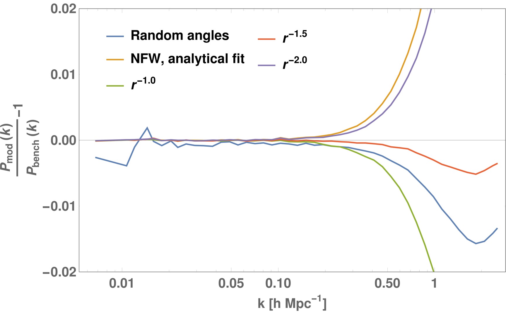
(a)

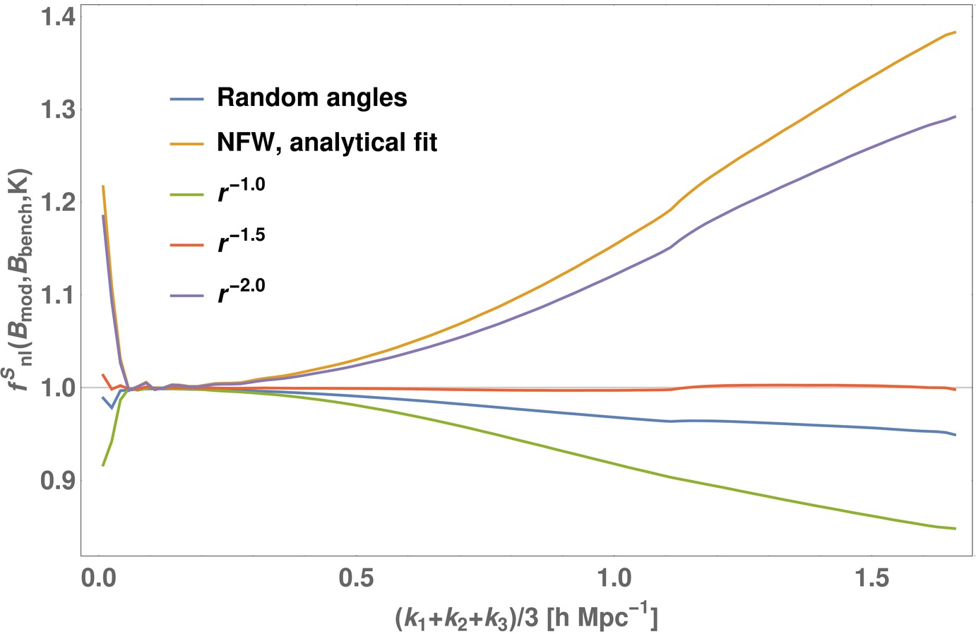
(b)

Figure IV.1: The relative power spectrum (left) and the sliced $f_{nl}$ bispectrum correlator (right) for different radial halo profile prescriptions for populating halos with subhalos. The power law profile $r^{-\gamma}$ is a much better fit to the actual subhalo distribution than the dark matter NFW profile, although the index $\gamma\approx 1$ suggested by the best fit to the true profile is power deficient. For $\gamma=1.5$ we obtain a near-perfect fit to both the power spectrum and bispectrum to high wavenumbers $k,K/3\leq 1.6\,h\,\text{Mpc}^{-1}$.

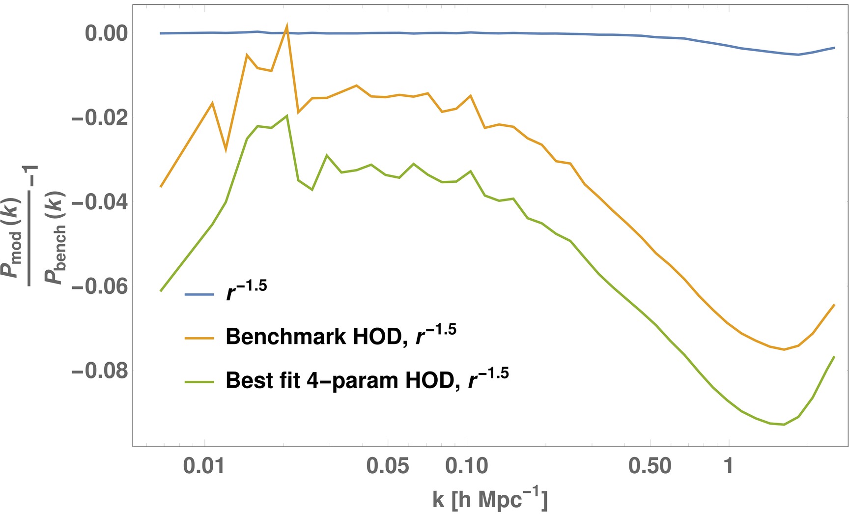
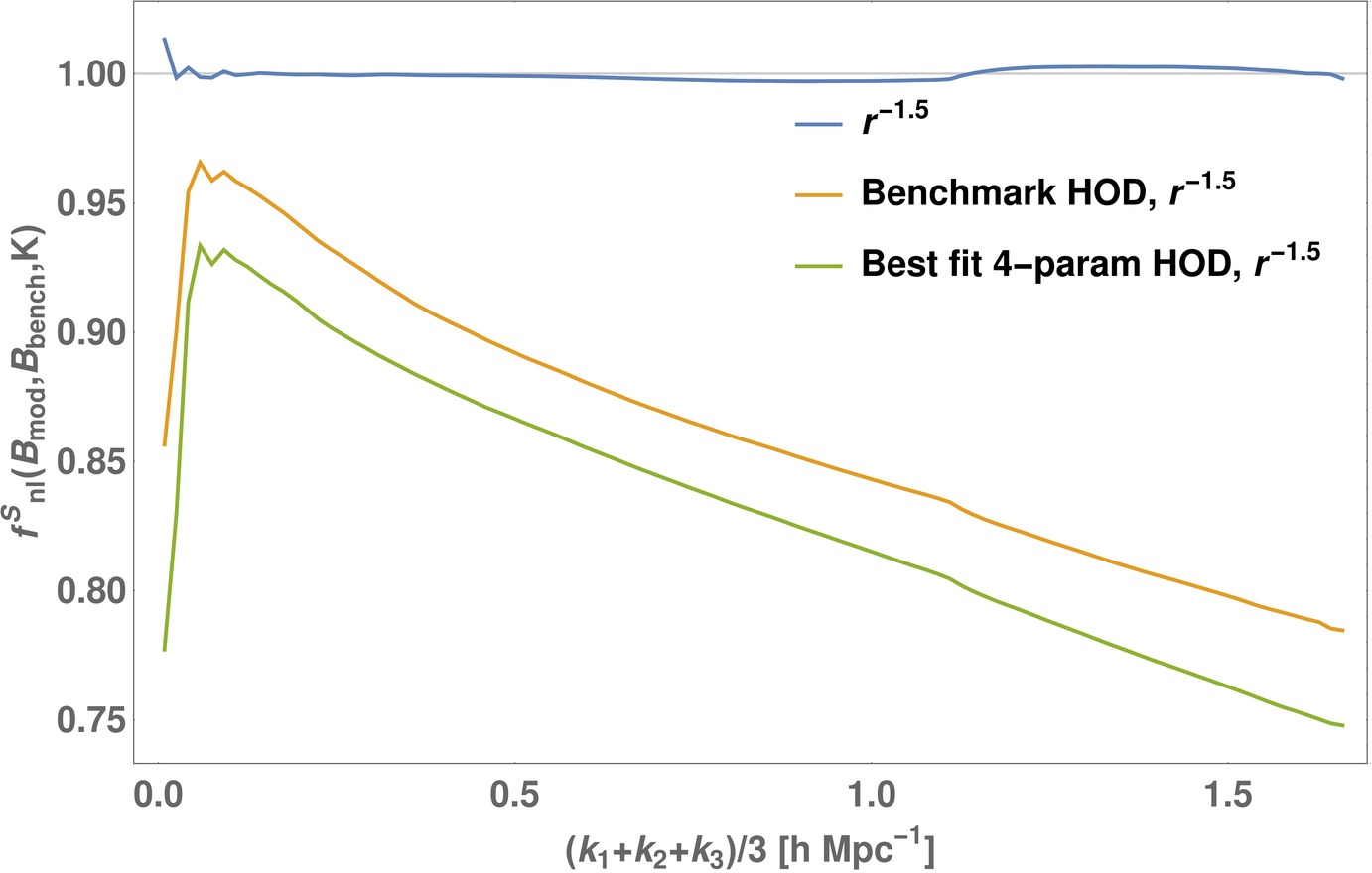
Figure IV.2: HOD prescriptions for statistically populating halos with subhalos yield a deficient power spectrum (left) and sliced bispectrum correlation (right). Neither the benchmark HOD nor the 4-parameter HOD model (using best fit parameters) can recover the benchmark power spectrum to better than 2% and the bispectrum to better than 4% at large scales, with much larger discrepancies on smaller scales.

Modifying the typical halo profile significantly impacts both the power spectrum and bispectrum, especially on small length scales. We can demonstrate (see below) this by keeping the number of subhalos fixed in each halo, while displacing their radial distribution according to a profile of our choosing (such as the popular NFW profile Equation II.3). First, however, we briefly study the importance of halo anisotropy. This was motivated by investigations of $N$-body simulations (such as that in Section II.2), which have revealed that the dark matter profiles of halos are not spherical, reflecting more complex internal substructure (Vega-Ferrero et al., 2017; Schneider et al., 2012; Vera-Ciro et al., 2011). The subhalos that live within those halos, therefore, also have a non-spherical distribution, as well as internal structure. We have quantified the importance of these effects by randomising the solid angular distribution of the subhalos within a halo, while keeping the radial distance to the parent halo seed unchanged. This effectively removes halo triaxiality, destroying the original internal structure of the halos. For the new ‘random angle’ halo catalogue, we have estimated both the power spectrum and the bispectrum (using the sliced $f_{nl}$ correlator (Equation III.12) at a given $K=k_{1}+k_{2}+k_{3}$); the relative effect is shown by the blue lines in Figure IV.1. There is a small diminution of power even at relatively high wavenumbers $k,K/3=1\,h\,\text{Mpc}^{-1}$, with less than a 1% and 4% decrease for the power spectrum and bispectrum respectively. Randomisation of the angles tends to reduce subhalo clustering but this remains a subpercent effect on the bispectrum for $K/3\leq 0.5\,h\,\text{Mpc}^{-1}$. The small effect of a randomisation process has on the matter power spectrum has also been confirmed in (Pace et al., 2015). This indicates that triaxial effects will predominantly arise from RSDs (see, for instance, (Smith et al., 2008)).

The radial halo profile can have a larger effect, notably if we populate subhalos using the NFW profile obtained from the halo dark matter distribution, as shown by the orange line in Figure IV.1. In this case, by $k,K/3=1\,h\,\text{Mpc}^{-1}$ there are large deviations of 2% and 15% from the halo power spectrum and bispectrum respectively. This is not unexpected as we have previously seen that the dark matter NFW profile does not fit the measured subhalo profile from our benchmark catalogue (given the mass resolution of our $N$-body simulation). The discrepancies would in fact have been even larger had we used the measured concentration from ROCKSTAR, instead of the analytical fit for $\expectationvalue{c}$ in Equation II.9.

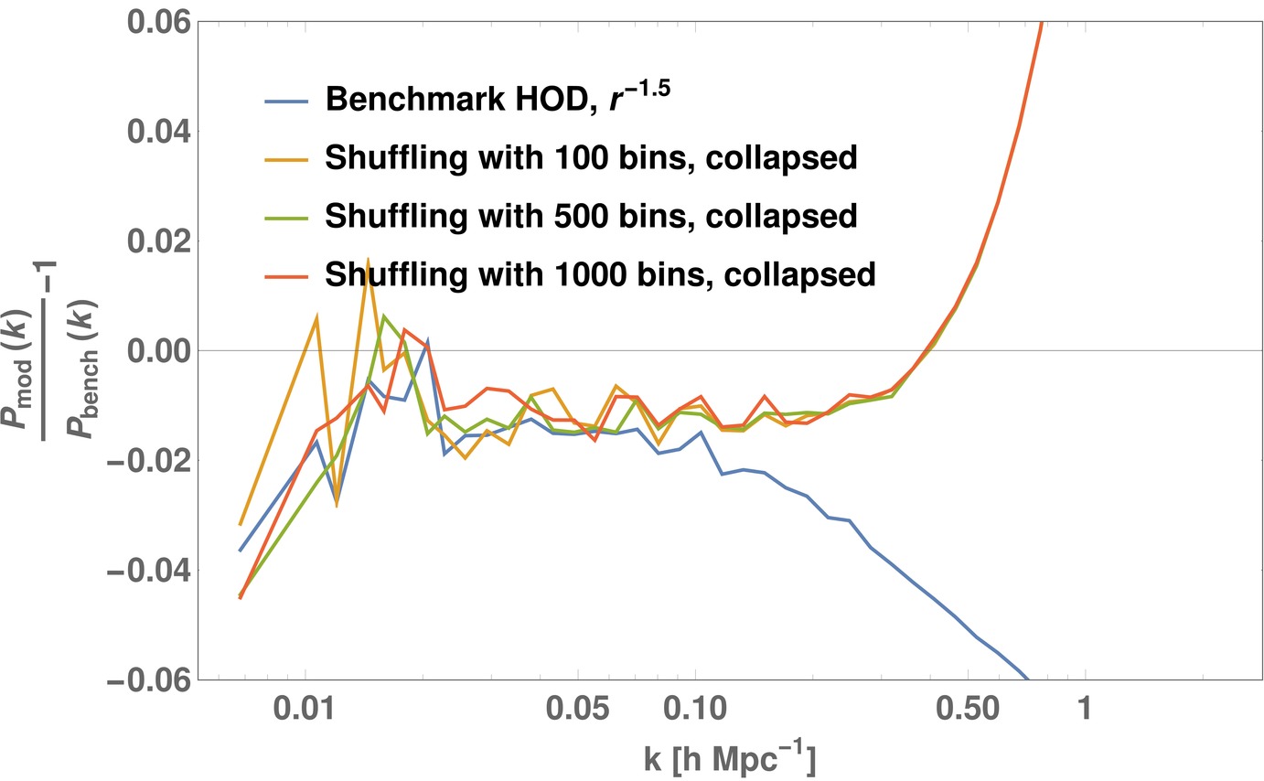
Figure IV.3: Shuffling the halo occupation number within a mass bin has the same effect as using the benchmark HOD.

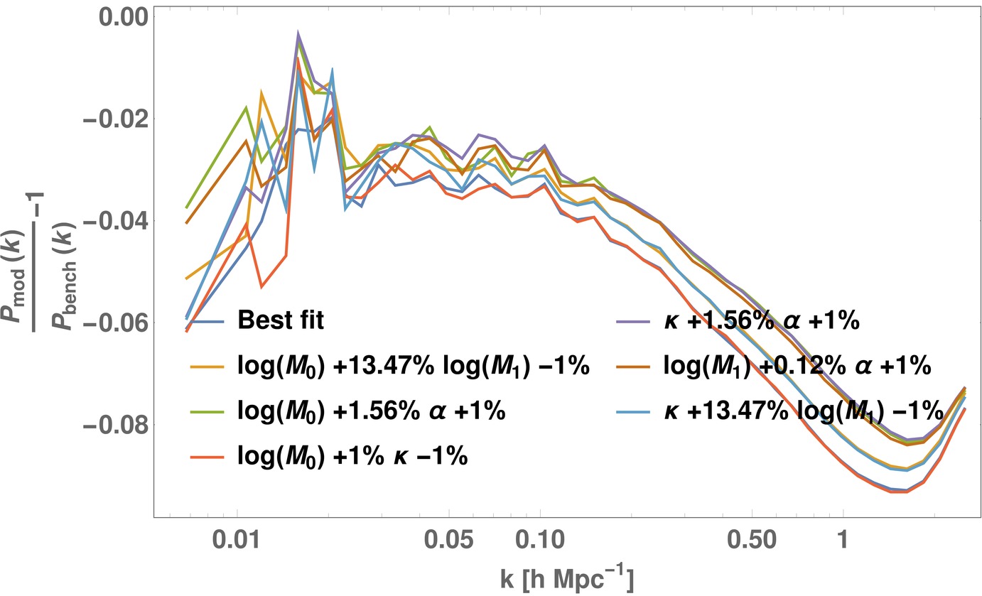
Figure IV.4: $\alpha$ has a strong influence on the power spectrum, unlike the other parameters. A radial profile $r^{-1.5}$ is used throughout.

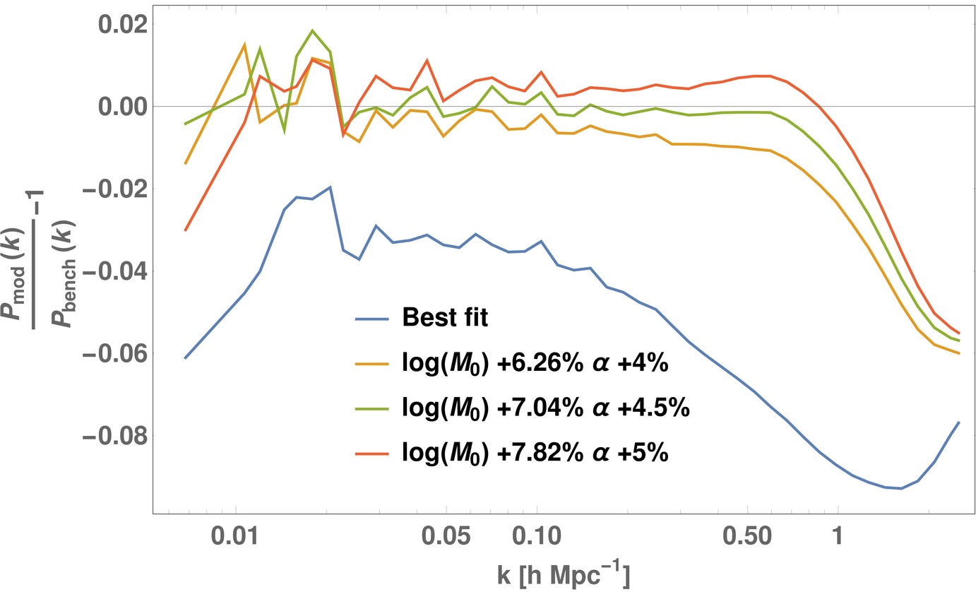
(a)

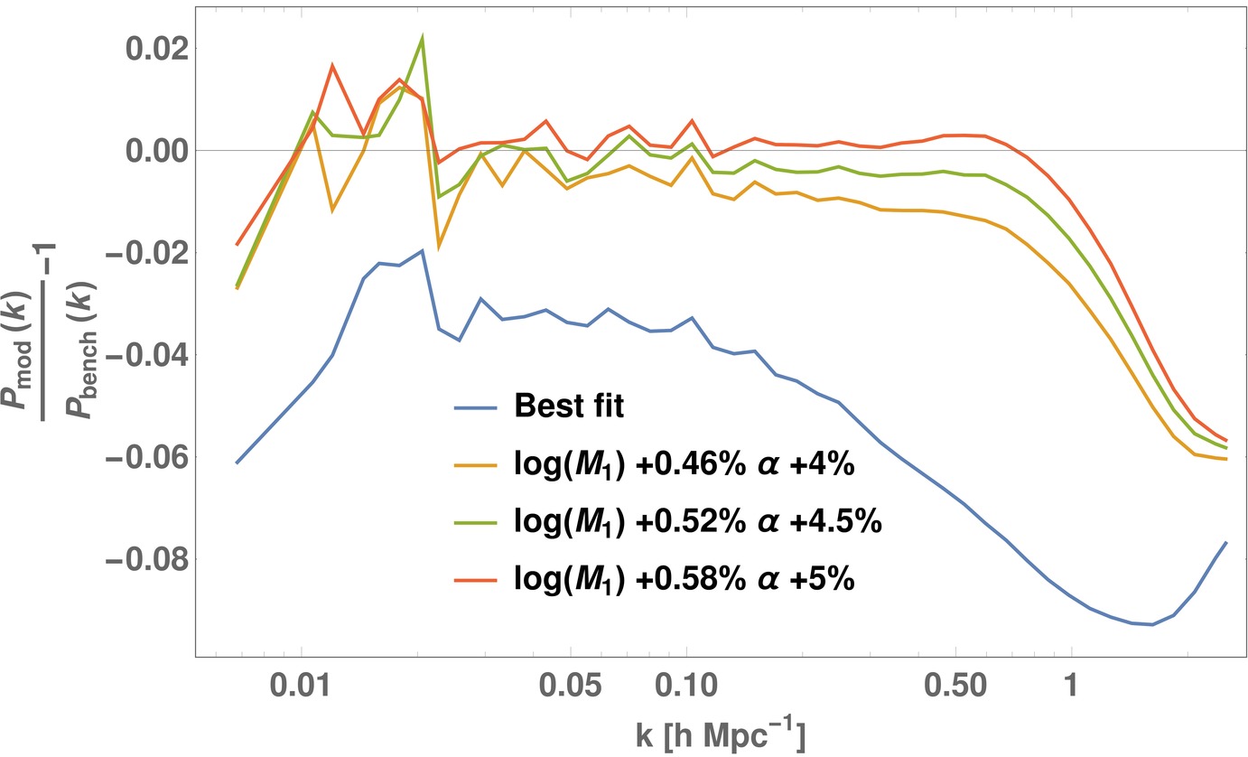
(b)

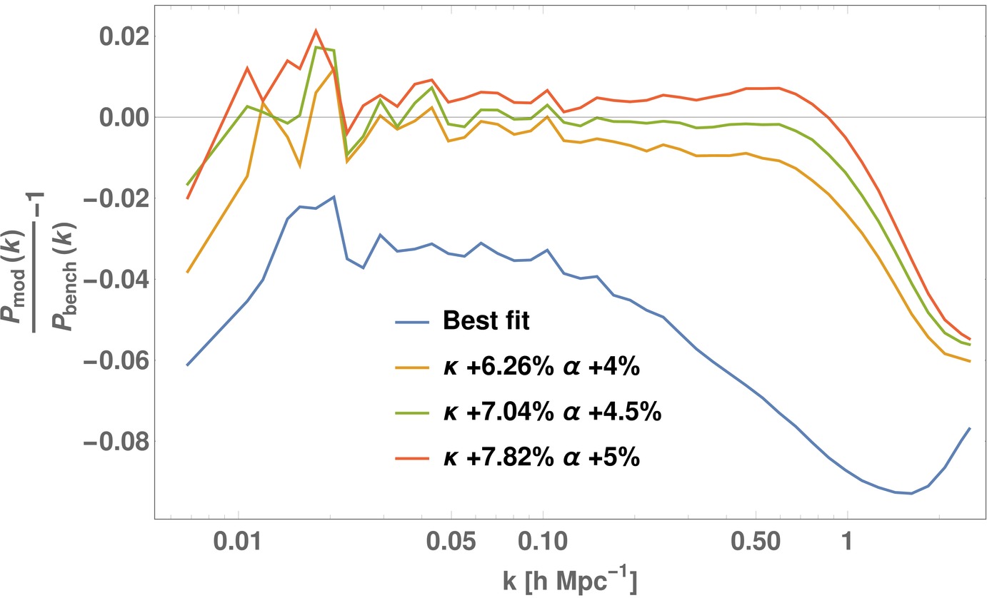
(c)

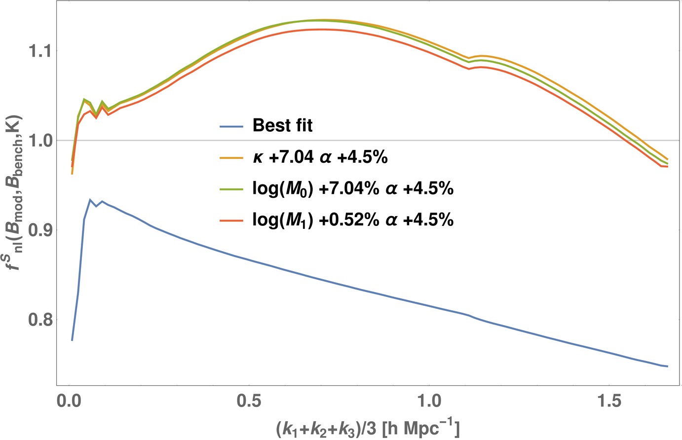
(d)

Figure IV.5: Panels (a)-(c): increasing $\alpha$ by 4.5% helps match the power spectrum to the benchmark, regardless of choice in the other parameter. Panel (d): the boost in power spectrum over-boosts the bispectrum.

We turn now to effects of modelling the halo profile with a power law. As we have seen already in Figure II.3, a power law of $0.8<\gamma<1.2$ will fit most halo profiles for the subhalo distributions found in our benchmark simulation. Modelling the halos with the best fit power law inevitably removes some signal from the power spectrum and bispectrum, as the resulting halos have a uniform solid angular distribution, unlike subhalos in an $N$-body simulation. The lack of power can be seen in the $\gamma=1$ profile shown as green line in Figure IV.1. We can phenomenologically compensate for this effect by considering spherically symmetric halo profiles with an increased power law exponent. Coincidentally, for $\gamma=1.5$ both the power spectrum and the bispectrum are very well fitted at all scales, with a difference of less than 0.5% up to $k,K/3\leq 1.6\,h\,\text{Mpc}^{-1}$. We can exploit this dual effect when populating the halos with a statistical halo occupation number rather than that measured from the $N$-body simulation.

Halo occupation number

(a) Benchmark ROCKSTAR catalogue

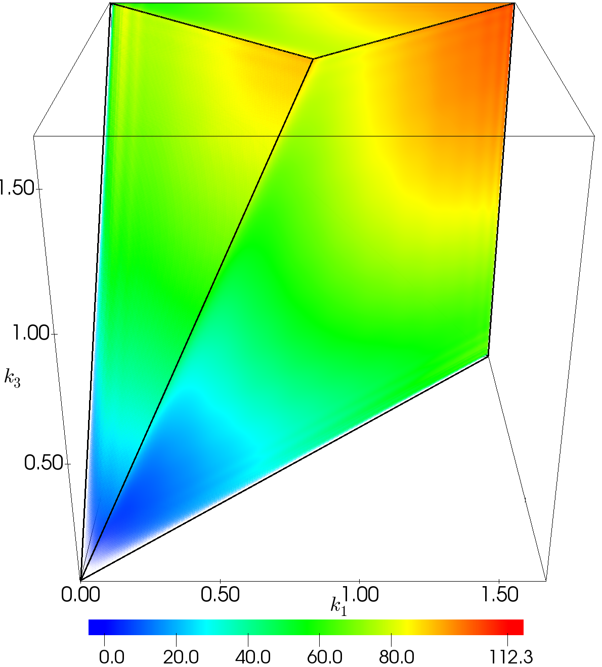
(b) Random solid angle

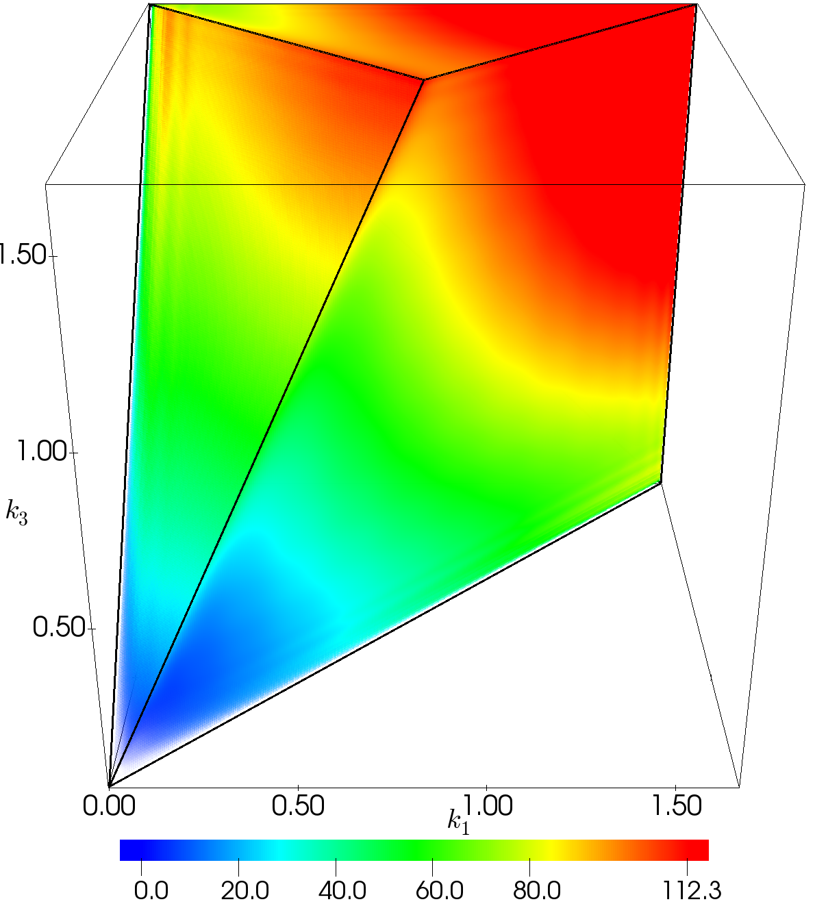
(c) NFW profile

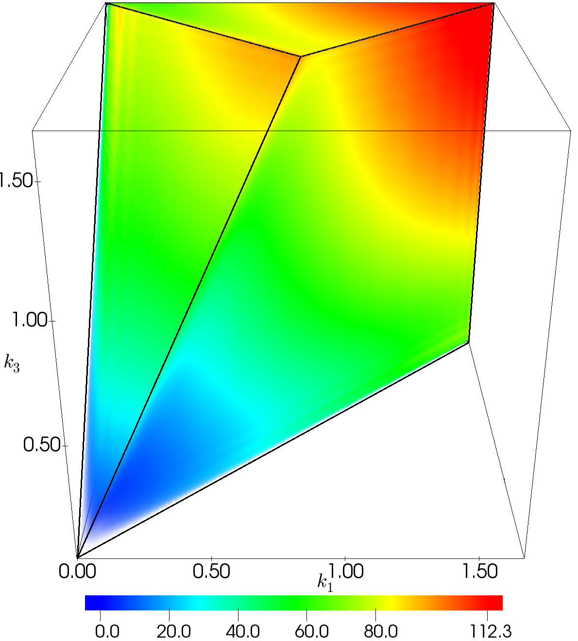
(d) Benchmark HOD and NFW profile

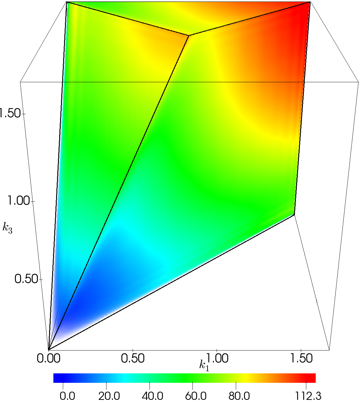
(e) Best fit 4-parameter HOD model

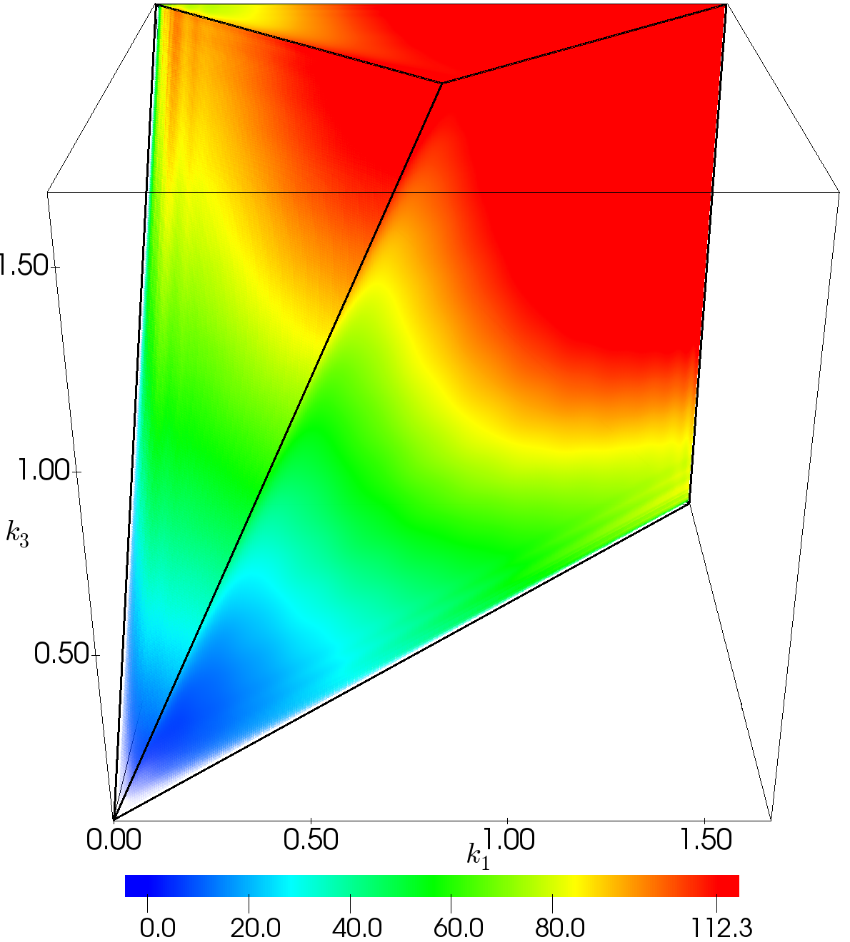
(f) 4-parameter HOD model, boost in $\alpha$ and $\kappa$

Figure IV.6: Bispectra of the simple galaxy mock catalogues.

We have also investigated the effect on the power spectrum and bispectrum of assigning subhalos using the Halo Occupation Distribution (HOD). First, we populated halos using the benchmark HOD model, i.e. we assigned to each halo the measured mean number of galaxies (subhalos) for a halo of that mass. This model is shown in Figure II.4 along with our 4-parameter fit to it. As shown in Figure IV.2, we have found that neither the benchmark HOD nor the 4-parameter HOD fit recovers the power spectrum or the bispectrum to better than 2% at large scales $k,K/3<0.1\,h\,\text{Mpc}^{-1}$. The 4-parameter fit to the benchmark HOD is 4% below the simulation power spectrum, and the difference gets rapidly worse at smaller length scales. The fit to the benchmark HOD is only accurate to 10%, indicating a better functional form should be adopted. The discrepancy in the bispectrum is considerably higher than the power spectrum, and also demonstrates much worse scaling in $k$.

To better understand the power deficiency observed in Figure IV.2 from using the HOD model we first binned the parent halos by mass, then shuffled around the halo occupation number within the halos in each mass bin. Since the halo profile plays only a marginal role on large length scales, for simplicity we collapsed all objects to the centre of the parent halo, and the power spectrum of the resulting sample is shown in Figure IV.4. The fact that this shuffling method, which preserves the statistical distribution of the halo occupation number in every mass bin, produces the same effect as the benchmark HOD strongly implies that number of subhalos in a halo depends on halo properties other than halo mass. The shuffling procedure is very similar to populating halos by using a subhalo dispersion around the mean HOD; initial experimentation indicated that including such a dispersion had no impact resolving the key bispectrum deficit.

Finally, we explored whether phenomenologically changing the parameters in our 4-parameter HOD could yield a satisfactory fit to both the power spectrum and bispectrum. As discussed in Section II.3 we enforce conservation of galaxy number $\Delta n_{g}=0$ (Section II.3) when changing the values of the parameters, which entails compensating by changing at least 2 parameters simultaneously. By exploring all 6 different ways to pair up the parameters, it was found that the index $\alpha$ in (Section II.3), i.e. the exponent of the power law, appears to make the most dramatic contribution to the power spectrum relative to the other parameters. As can be seen in panels (a)-(c) in Figure IV.5, boosting $\alpha$ by 4.5% helps match the benchmark power spectrum up to $k\leq 0.5\,h\,\text{Mpc}^{-1}$, regardless of the choice of the other compensating parameter. However, panel (d) in the same plot reveals that this boost in $\alpha$ grossly inflates the bispectrum, resulting in more than 5% difference between $0.2\,h\,\text{Mpc}^{-1}<K/3<1.3\,h\,\text{Mpc}^{-1}$. We conclude that populating halos using an HOD that depends only on mass will not simultaneously recover both the benchmark power spectrum and bispectrum (with correlation discrepancies in the latter exceeding 4%).

Assembly bias

Since using the benchmark HOD yields a suppression of power in the power spectrum and bispectrum, and tuning the 4-parameter HOD model fares no better in matching both the power spectrum and bispectrum, we considered alternative methods of modelling the halo occupation number that take into account the formation history of the halos, known as assembly bias (see, for example, (Vakili and Hahn, 2019; Gao et al., 2005; Sunayama et al., 2016; Hearin et al., 2016; Wechsler et al., 2006)). Amongst halos with the same mass those formed at higher redshifts in $N$-body simulations are known to typically have higher concentrations $c$ (Zhao et al., 2003, 2009; Villarreal et al., 2017; Wechsler et al., 2002, 2006) (although this relationship should not be over-simplified (Mao et al., 2017)). For this reason, we investigate whether incorporating halo concentration into our HOD model can simultaneously reduce the measured mock catalogue deficit in both the power spectrum and bispectrum. The probability distribution of the occupation number $N_{g}$ becomes $P(N_{g}|c,M)$, which is a function of both mass and concentration.

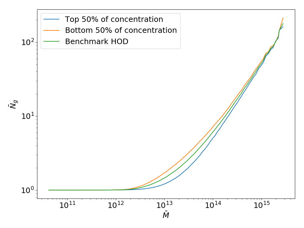
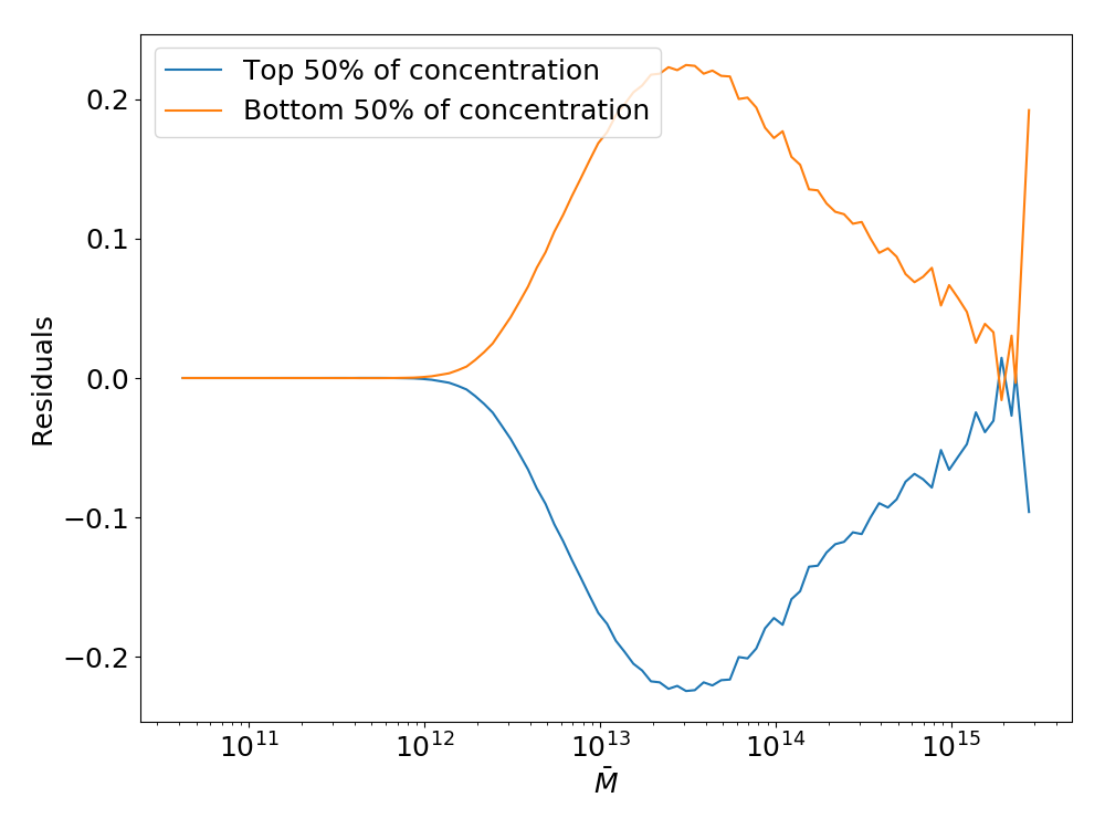
Figure IV.7: Left panel: We separate halos within a mass bin into 2 samples split by the median concentration, and calculate their average halo occupation. Right panel: Residuals of those 2 samples relative to the benchmark HOD.

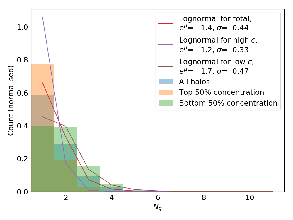
(a) $M=(0.62-2.2)\times 10^{13}h^{-1}\,M_{\odot}$

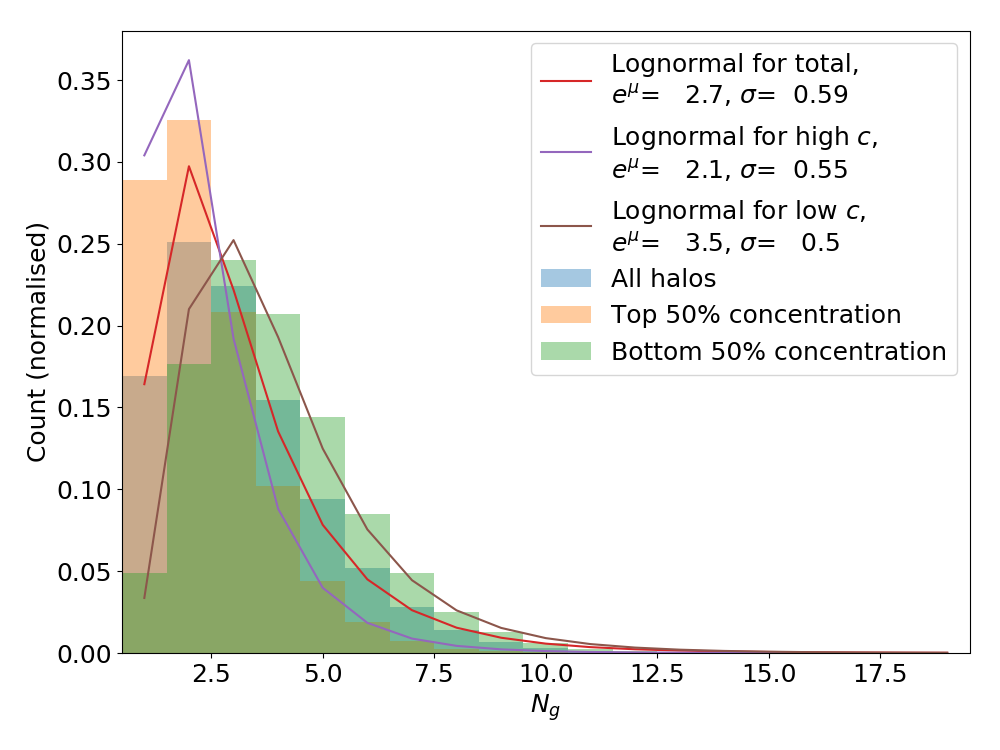
(b) $M=(2.2-7.6)\times 10^{13}h^{-1}\,M_{\odot}$

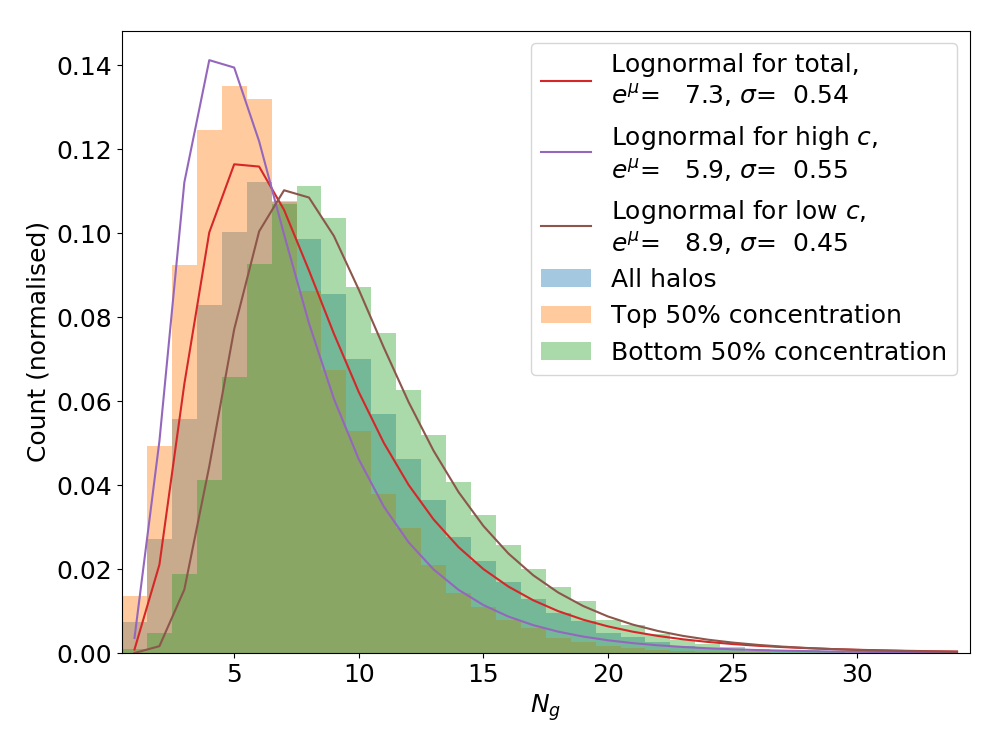
(c) $M=(0.76-2.7)\times 10^{14}h^{-1}\,M_{\odot}$

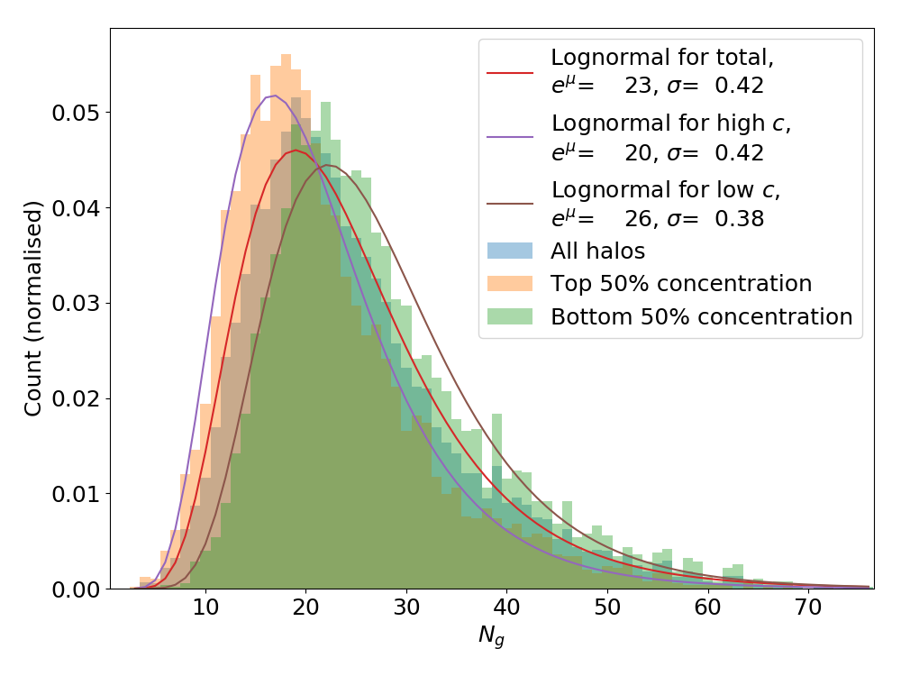
(d) $M=(2.7-9.3)\times 10^{14}h^{-1}\,M_{\odot}$

Figure IV.8: The standard lognormal distribution fitted to the total halo occupation number, as well as the occupation number for the high and low concentration bins.

To gain insight into how the concentration affects halo occupation we took inspiration from (Eisenstein et al., 2018) with a simple model that, first, bins parent halos by mass and then, secondly, divides these into two bins based on their concentration. The threshold for this split into concentration bins was the median concentration, such that both the higher and the lower concentration samples at a given mass have the same number of subhalos. For each mass bin, we calculated the mean occupation number in the high and low concentration bins (as well as the whole sample). Figure IV.7 shows that halos with lower concentration clearly have more subhalos than the average, amounting to a 20% difference in the mass range between of $10^{13}h^{-1}\,M_{\odot}$ and $10^{14}h^{-1}\,M_{\odot}$. The significant anticorrelation of the concentration with the number of subhalos may or may not be reflected in actual galaxy distributions because of resolution limitations and absent dynamical effects in our DM-only $N$-body simulations. If halos with high concentration are indeed typically those that are formed earlier, then the lower number of subhalos will be affected by merging of substructure which is, in turn, influenced by halo resolution (see, for example, (Stewart et al., 2009)).

The positive impact of accounting for concentration with this simple split bin model is illustrated in Figure IV.15 for both the power spectrum and bispectrum. Here, we have populated halos with subhalos drawn from a lognormal distribution to model the total occupation number of the two concentration bins at each mass scale (see below). These results should be compared with the benchmark HOD model in Figure II.4 where the bispectrum was very discrepant. In particular, this reduces the deficit in the bispectrum from around 6% to 3% at $K/3=0.2\,h\,\text{Mpc}^{-1}$, so assembly bias is clearly an important factor which should be taken into account when creating mock catalogues.

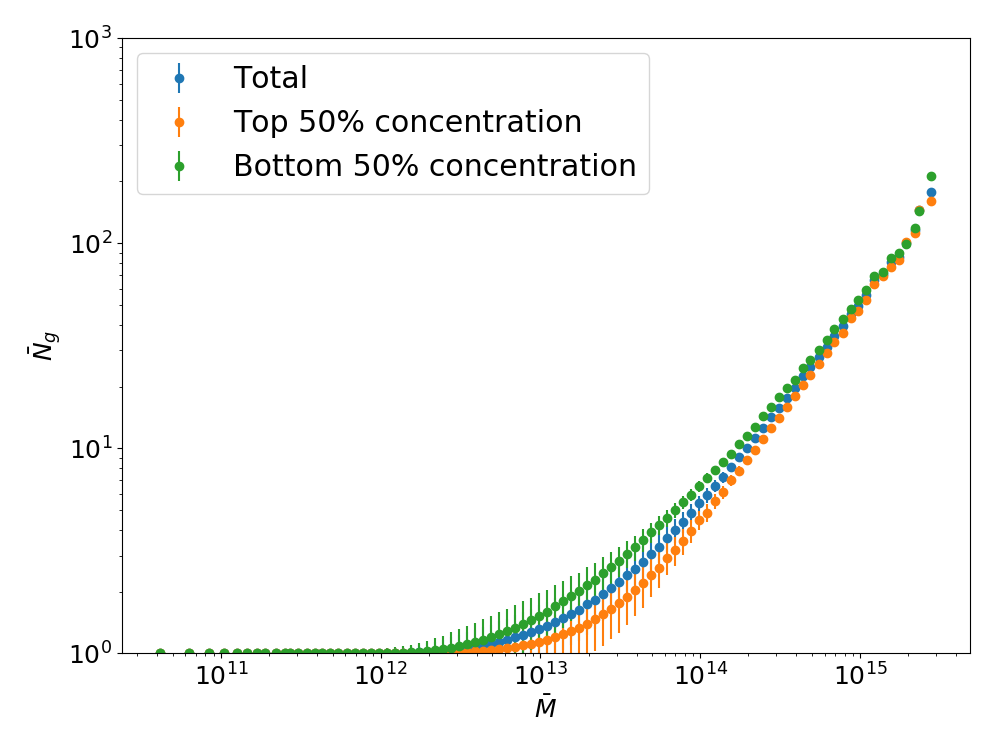
Figure IV.9: Lognormal fits to the total occupation number and the high and low concentration bins. The vertical error bars indicate the shape parameter $\sigma$ of the fits.

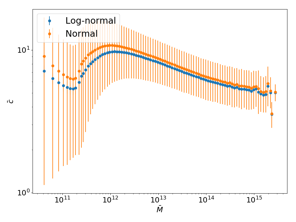
(a)

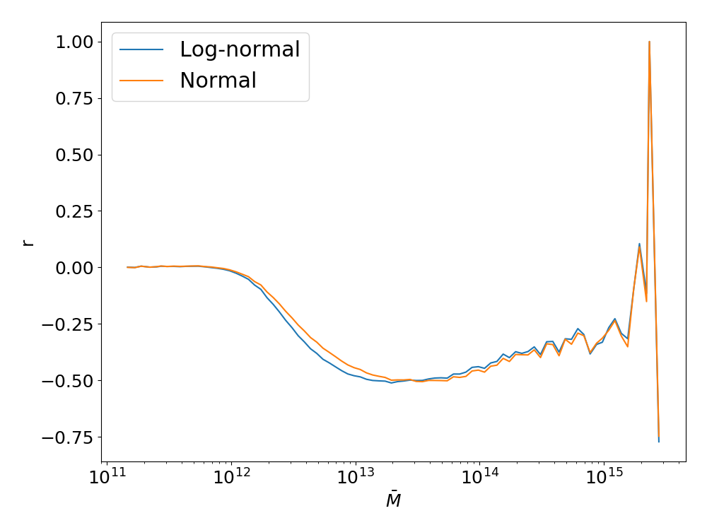
(b)

Figure IV.10: Left panel: Lognormal and Gaussian fits to $\bar{c}$. The vertical error bars indicate the shape parameter $\sigma$ of the fits. Right panel: Correlation coefficient $r$ of the bivariate Gaussian distribution between $\ln(N_{g})$ and $X$.

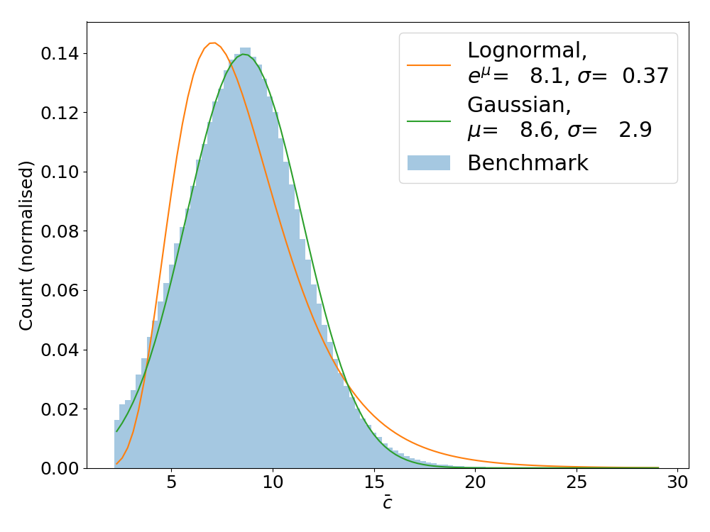
(a) $M=(0.62-2.2)\times 10^{13}h^{-1}\,M_{\odot}$

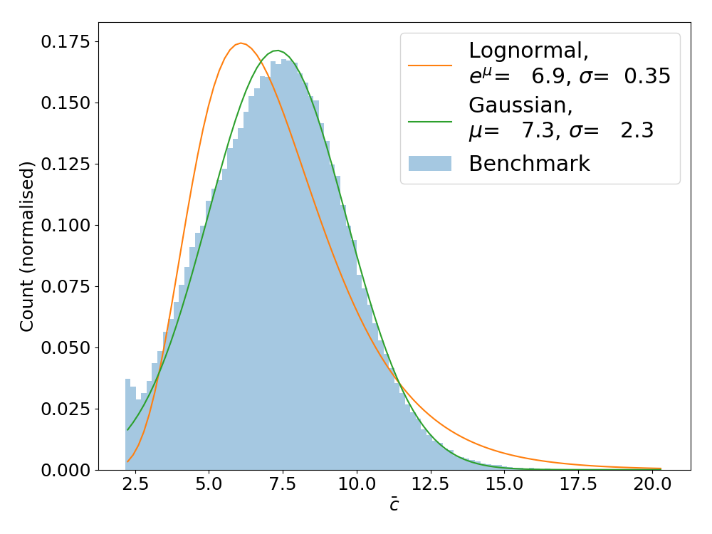
(b) $M=(2.2-7.6)\times 10^{13}h^{-1}\,M_{\odot}$

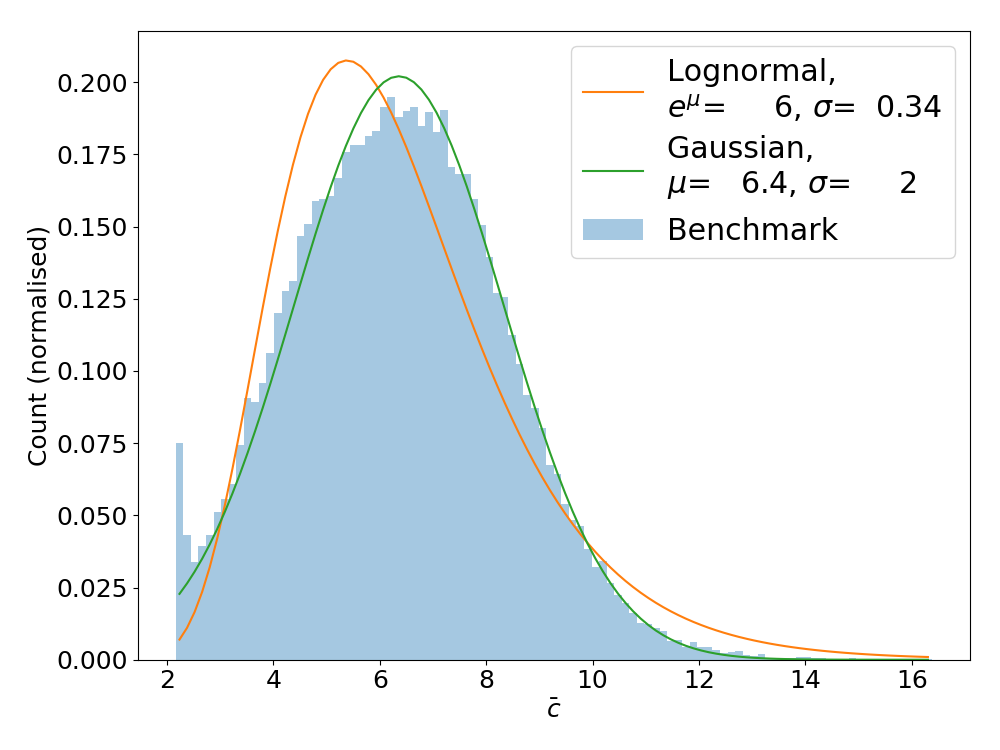
(c) $M=(0.76-2.7)\times 10^{14}h^{-1}\,M_{\odot}$

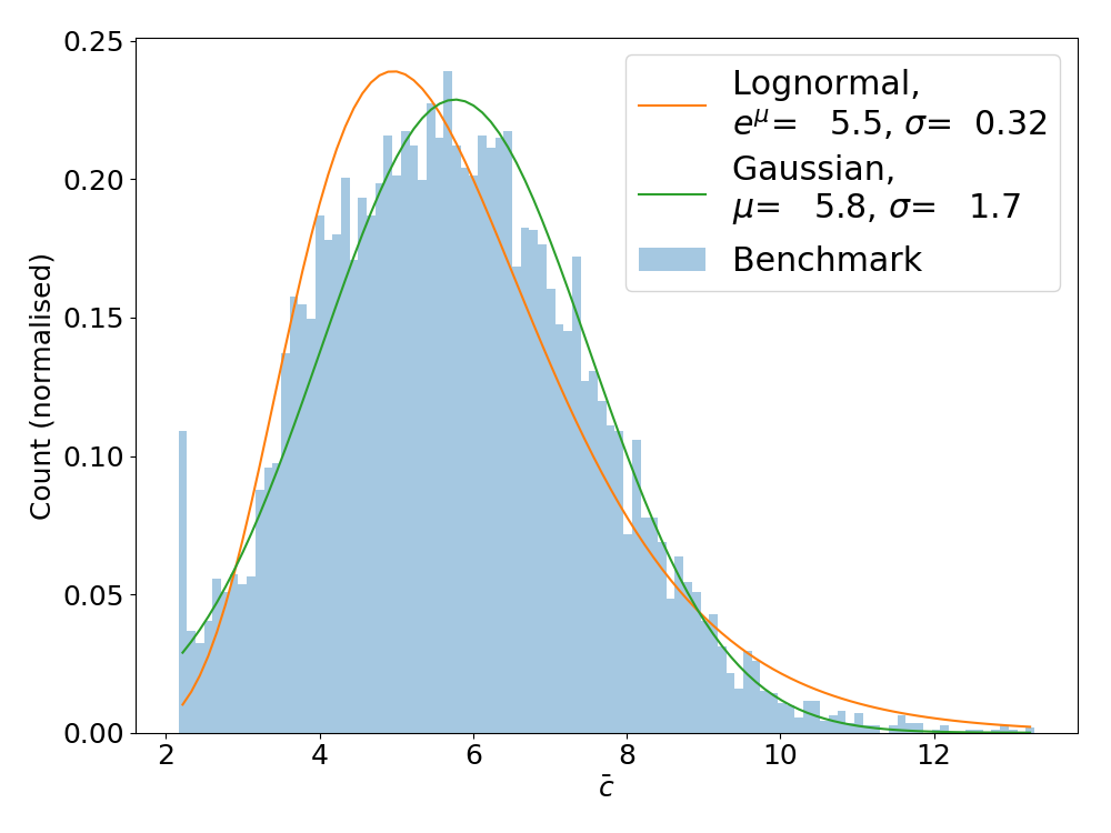
(d) $M=(2.7-9.3)\times 10^{14}h^{-1}\,M_{\odot}$

Figure IV.11: A lognormal distribution is too skewed to model the distribution of halo concentration, but a Gaussian fits very well especially at low mass.

In light of the impact of concentration on subhalo number, our goal is to develop a more sophisticated statistical model that allows us to populate individual halos of a given mass, with or without specifying the concentration from information given by the simulation. To achieve this, we require the joint probability distribution $P(N_{g}\cap c\,|M)$ as a function of subhalo number $N_{g}$ and concentration $c$, so that we can derive $P(N_{g}|c,M)$ from Bayes theorem (Bayes and Price, 1763):

$$P(N_{g}|c,M)=\frac{P(N_{g}\cap c\,|M)}{P(c|M)}.$$ (IV.1)

To find an appropriate joint distribution we first investigate the marginalised distributions for $N_{g}$ and $c$. It was found that the standard lognormal distribution with 2 parameters, $\text{Lognormal}(\mu,\sigma^{2})$ where $e^{\mu}$ is known as the scale parameter and $\sigma$ the shape parameter, provides a good fit to the marginalised halo occupation number. Figure IV.8 shows the lognormal fits to the total occupation number, and occupation number in the high and low concentration bins, for several mass bins. In Figure IV.9 we show the shape and scale parameters of these fits in 100 mass bins across the whole range of the benchmark catalogue. Note that we have adopted the total occupation number, i.e. including the central galaxy instead of just the satellites, because when the average number of satellites falls below unity the lognormal fit automatically fails.

For the marginalised concentration distribution, we found that it could be more accurately modelled with a Gaussian distribution, particularly at low masses. The lognormal distribution provides a significantly worse fit, a comparison which is shown in Figure IV.11, where we display the normalised counts in several mass bins along with the best fit values for both Gaussian and lognormal fits.

Either the Gaussian or lognormal distributions for $c$ can be easily combined with the lognormal distribution for $N_{g}$ to give a joint distribution. To do so we simply have to take the natural logarithm of $N_{g}$ and calculate the mean $\boldsymbol{\mu}$ and covariance $\boldsymbol{\Sigma}$ for this joint Gaussian distribution:

$$\begin{pmatrix}\ln(N_{g})\\ X\end{pmatrix}\sim\mathcal{N}(\boldsymbol{\mu},\boldsymbol{\Sigma}),$$ (IV.2)

where $X=c$ or $\ln(c)$ depending on whether a Gaussian or lognormal distribution for $c$ is desired, and

$$\boldsymbol{\mu}=\begin{pmatrix}\expectationvalue{\ln(N_{g})}\\ \expectationvalue{X}\end{pmatrix},\qquad\boldsymbol{\Sigma}=\begin{pmatrix}\sigma^{2}_{\ln(N_{g})}&\sigma_{\ln(N_{g}),X}\\ \sigma_{\ln(N_{g}),X}&\sigma^{2}_{X}\end{pmatrix}.$$ (IV.3)

$\sigma^{2}_{\ln(N_{g})}$ and $\sigma^{2}_{X}$ are the usual variances for $\ln(N_{g})$ and $X$, and $\sigma_{\ln(N_{g}),X}=\expectationvalue{(\ln(N_{g})-\expectationvalue{\ln(N_{g})})(X-\expectationvalue{X})}$ is the covariance between them.

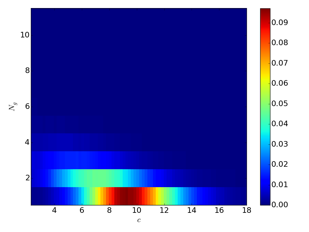
(a) $M=(0.62-2.2)\times 10^{13}h^{-1}\,M_{\odot}$

(b) $M=(2.2-7.6)\times 10^{13}h^{-1}\,M_{\odot}$

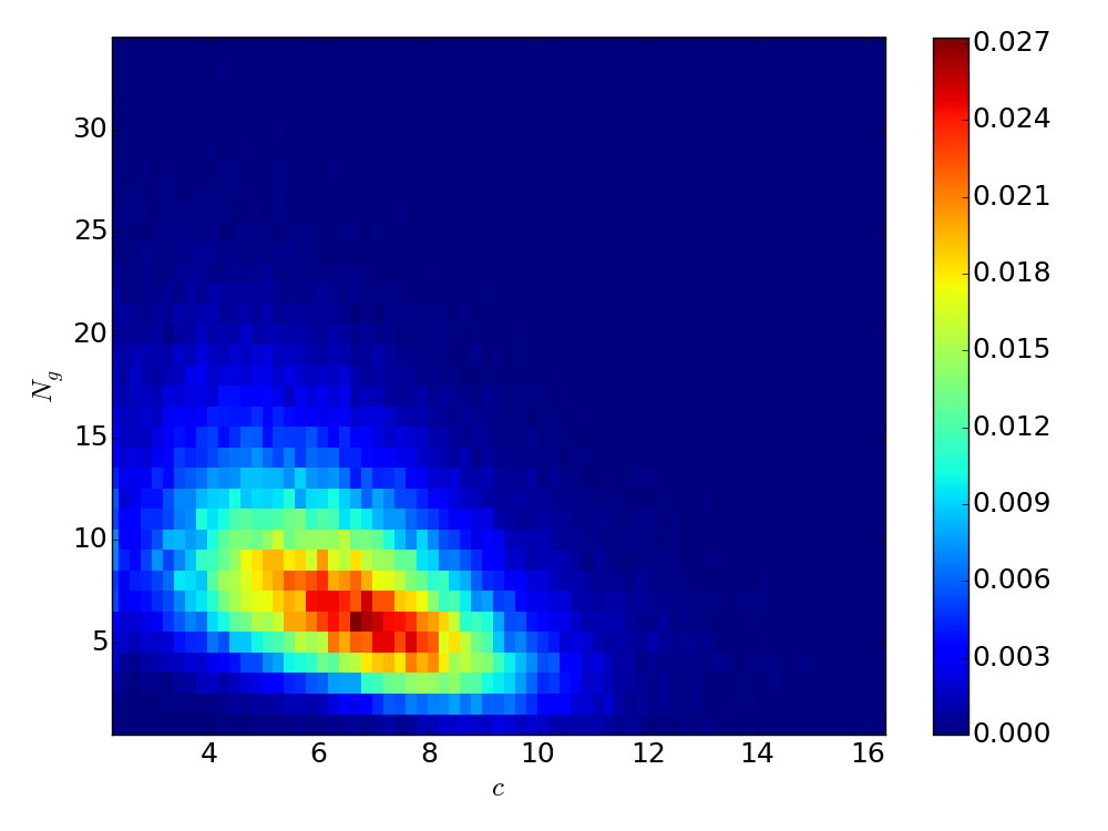
(c) $M=(0.76-2.7)\times 10^{14}h^{-1}\,M_{\odot}$

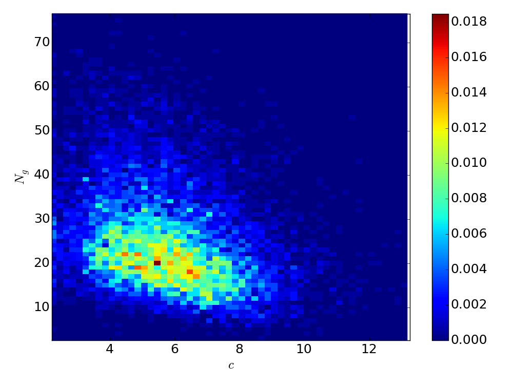
(d) $M=(2.7-9.3)\times 10^{14}h^{-1}\,M_{\odot}$

Figure IV.12: Joint probability distribution for the subhalo number $N_{g}$ and concentration $c$ for halos in different mass bins of the benchmark ROCKSTAR catalogue.

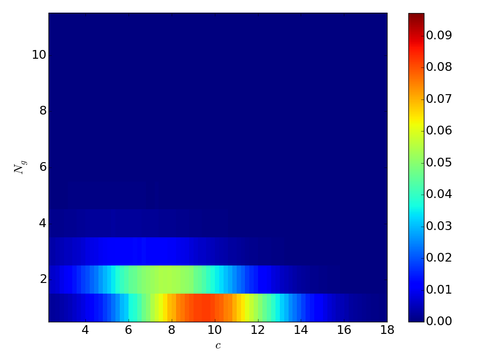
(a) $M=(0.62-2.2)\times 10^{13}h^{-1}\,M_{\odot}$

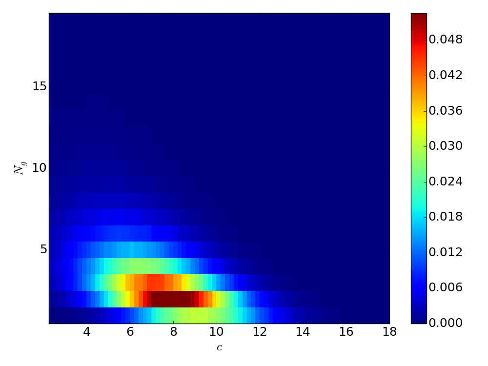
(b) $M=(2.2-7.6)\times 10^{13}h^{-1}\,M_{\odot}$

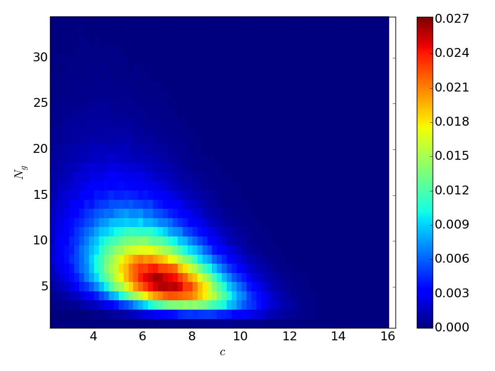
(c) $M=(0.76-2.7)\times 10^{14}h^{-1}\,M_{\odot}$

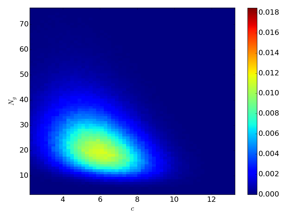
(d) $M=(2.7-9.3)\times 10^{14}h^{-1}\,M_{\odot}$

Figure IV.13: Joint lognormal-Gaussian fit to the joint distribution in Figure IV.12 which should be compared with benchmark distribution shown in Figure IV.12.

To draw from the joint distribution one would then sample from the joint Gaussian distribution and exponentiate the result as required. The joint distribution obtained from the ROCKSTAR halo benchmark is shown for various mass bins in Figure IV.12. For comparison, we show for the same mass bins calculated both from the joint lognormal distribution in Figure IV.14 and from the joint lognormal-Gaussian distribution in Figure IV.13. The joint lognormal-Gaussian distribution appears to reproduce the benchmark distribution more accurately, though small discrepancies remain at high mass.

In order to obtain $P(N_{g}|M,c)$ we first shift the distribution for $\ln(N_{g})$ from $\mathcal{N}(\expectationvalue{\ln(N_{g})},\sigma^{2}_{\ln(N_{g})})$ to $\mathcal{N}(\expectationvalue{\ln(N_{g})}^{\prime},\sigma^{\prime 2}_{\ln(N_{g})})$, where (Eaton, 1983)

$$\expectationvalue{\ln(N_{g})}^{\prime} =\expectationvalue{\ln(N_{g})}+\frac{\sigma_{\ln(N_{g}),X}}{\sigma^{2}_{X}}(X-\expectationvalue{X})$$ (IV.4)

$$\sigma^{\prime 2}_{\ln(N_{g})} =\sigma^{2}_{\ln(N_{g})}-\frac{\sigma^{2}_{\ln(N_{g}),X}}{\sigma^{2}_{X}},$$ (IV.5)

then exponentiate draws from this shifted Gaussian distribution. This shift can be derived using the bivariate Gaussian distribution in Equation IV.2, the Gaussian distribution for $X$ and Bayes theorem (Equation IV.1). For the benchmark catalogue in Figure IV.10(a) we show the parameters of the lognormal and Gaussian fits to $c$, and the correlation coefficient

$$r=\frac{\sigma_{\ln(N_{g}),X}}{\sqrt{\sigma_{\ln(N_{g})}\sigma_{X}}}$$ (IV.6)

obtained for the joint Gaussian distribution in Figure IV.10(b). It is worth noting that there are only minor differences in the correlation coefficient between the Gaussian and lognormal cases, with a robust value of around $r\approx-0.5$ found for the mass range $M=10^{13}-10^{14}h^{-1}\,M_{\odot}$.

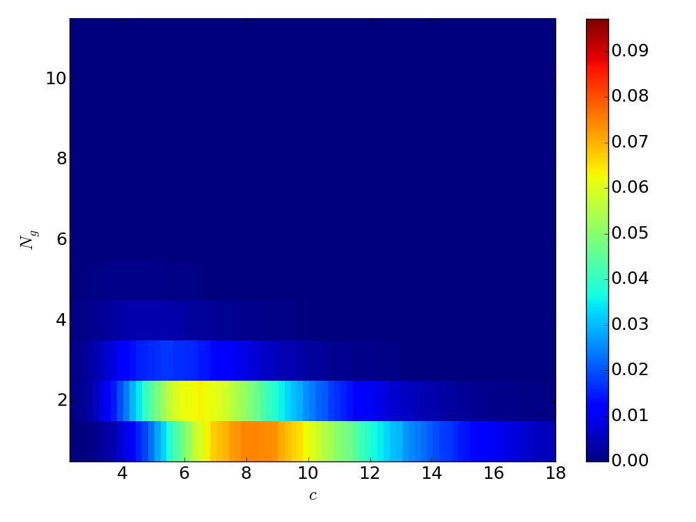
(a) $M=(0.62-2.2)\times 10^{13}h^{-1}\,M_{\odot}$

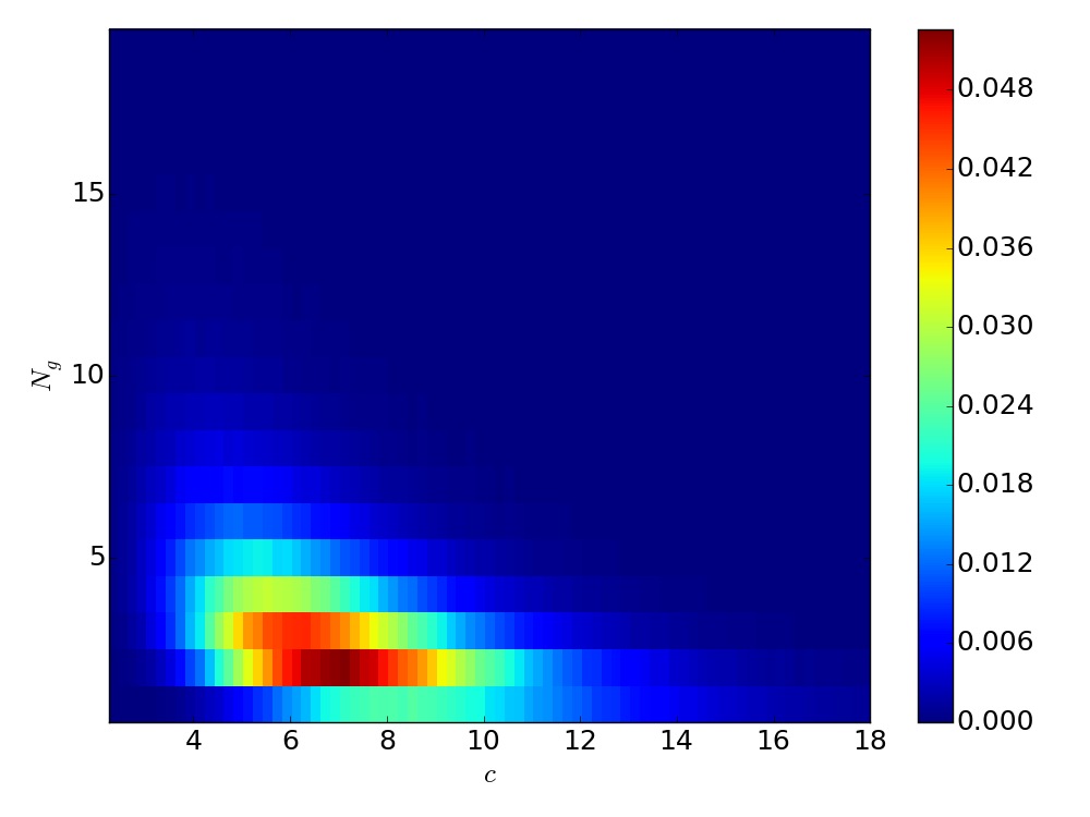
(b) $M=(2.2-7.6)\times 10^{13}h^{-1}\,M_{\odot}$

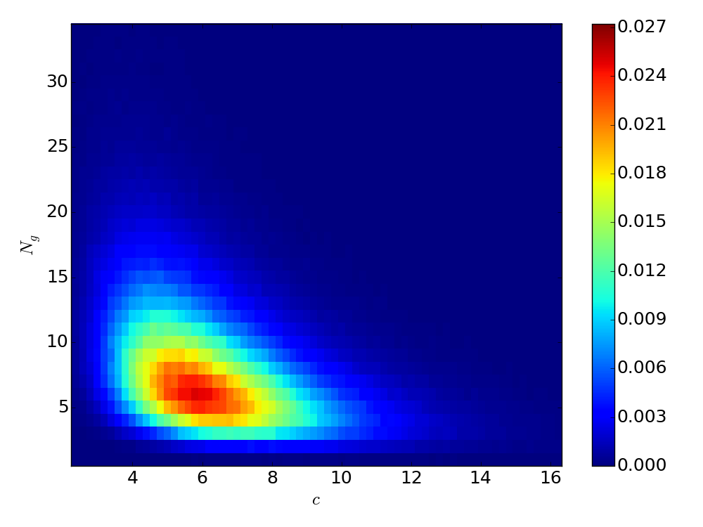
(c) $M=(0.76-2.7)\times 10^{14}h^{-1}\,M_{\odot}$

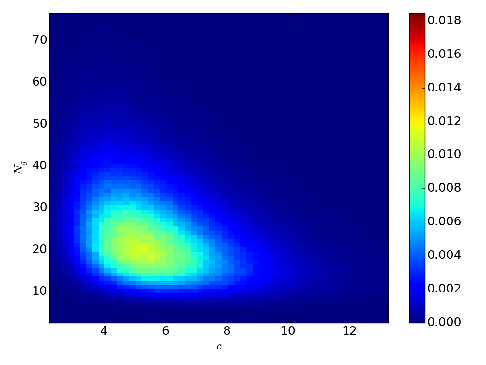
(d) $M=(2.7-9.3)\times 10^{14}h^{-1}\,M_{\odot}$

Figure IV.14: Joint lognormal fit to the joint distribution in Figure IV.12.

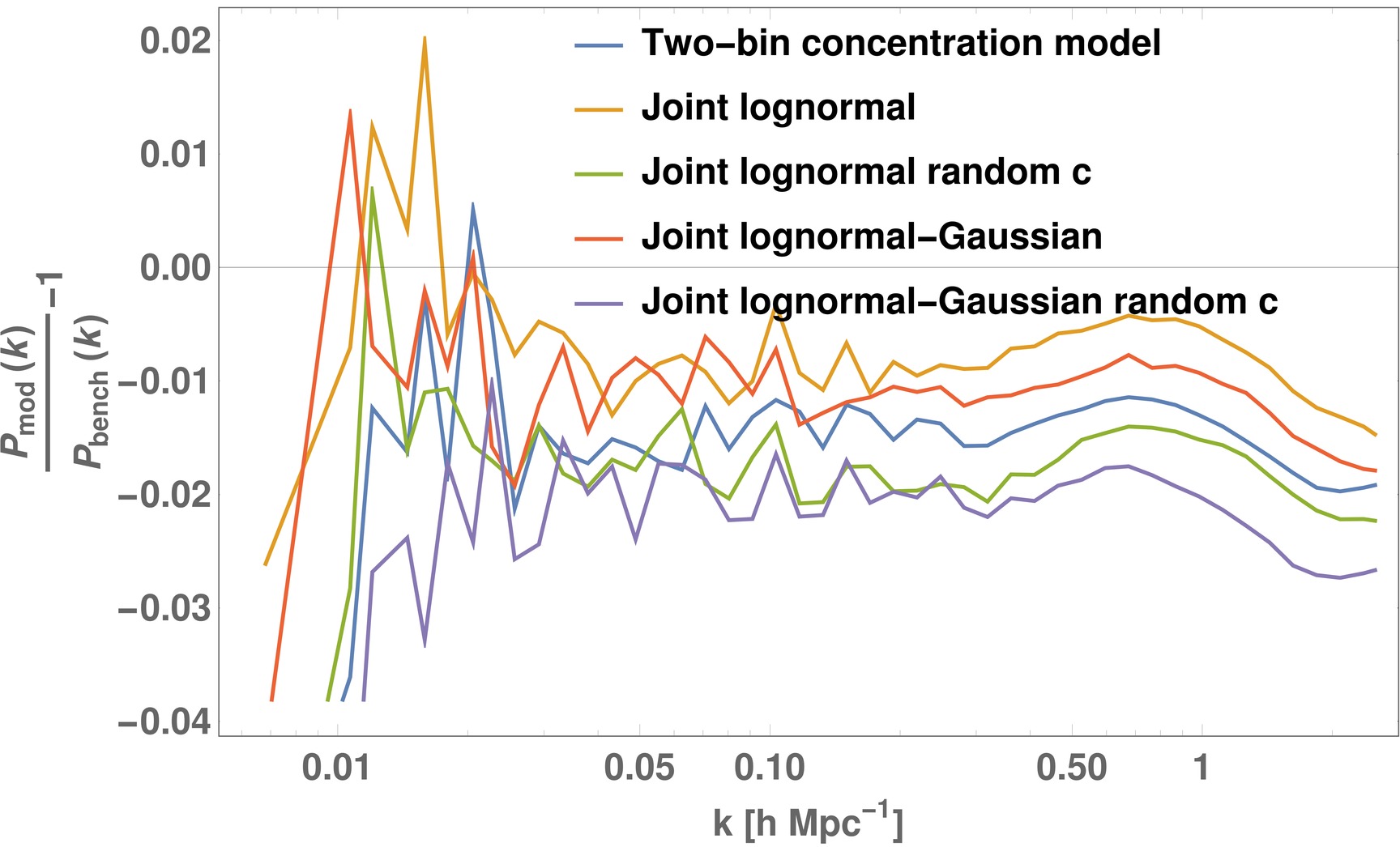
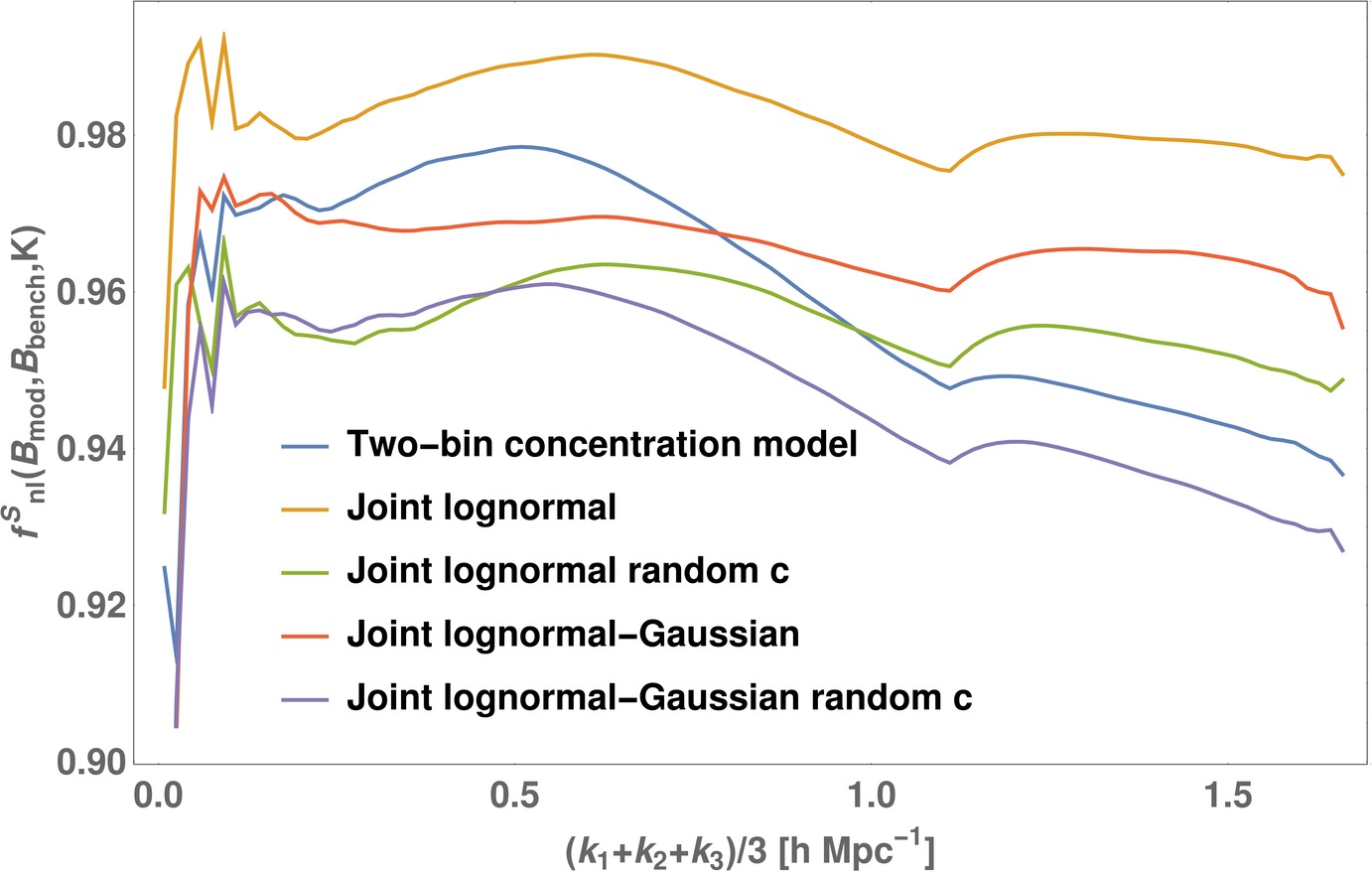
Figure IV.15: Power spectra (left) and bispectra (right) comparisons of the two-bin and joint distribution assembly bias HOD models relative to the measured benchmark polyspectra. Prescriptions using the joint probability distribution and information about the individual halo concentrations improve the fit to better than 2% for $k<1.0\,h\,\text{Mpc}^{-1}$. The halo profile adopted here is a power law with $\gamma=1.5$.

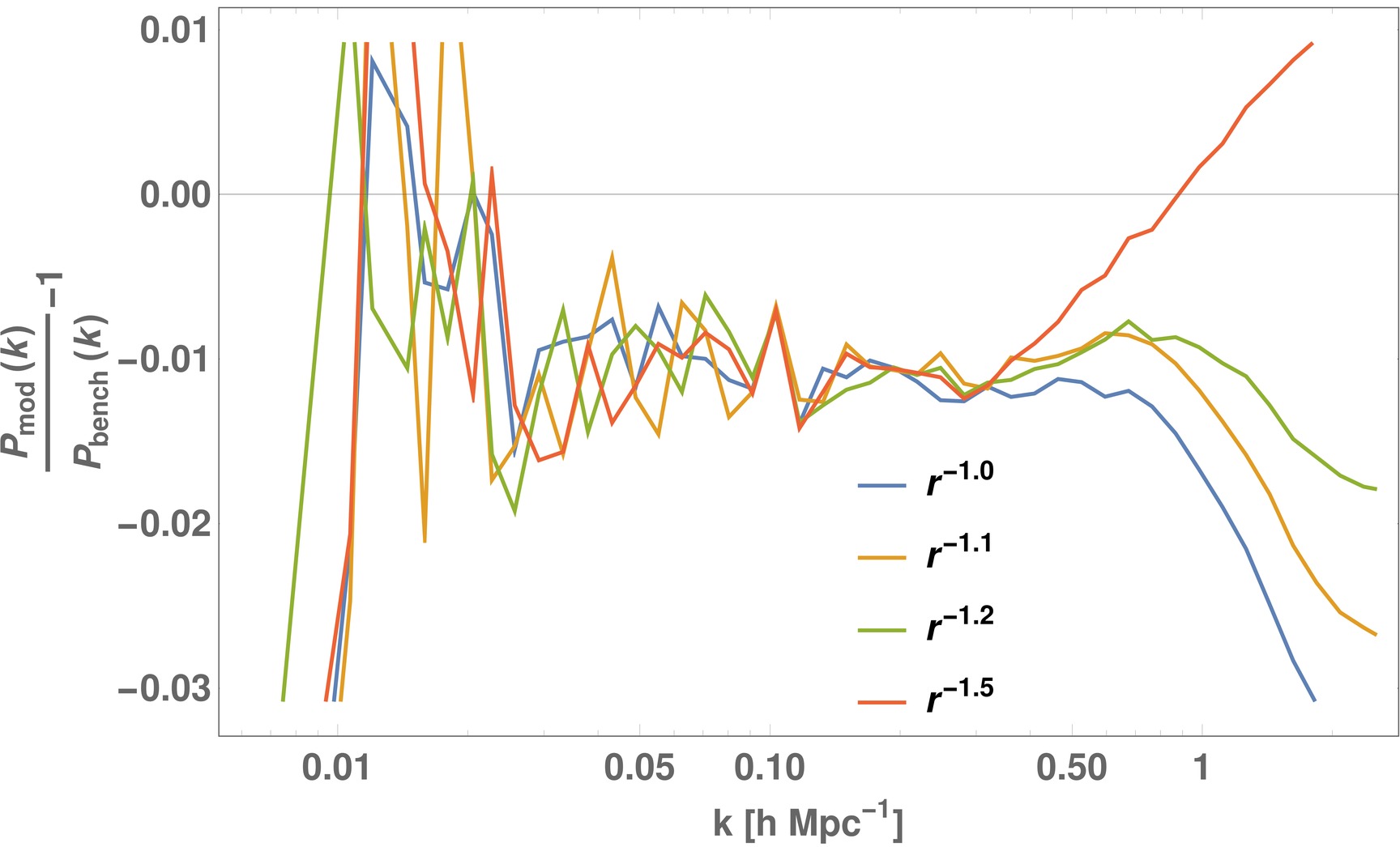
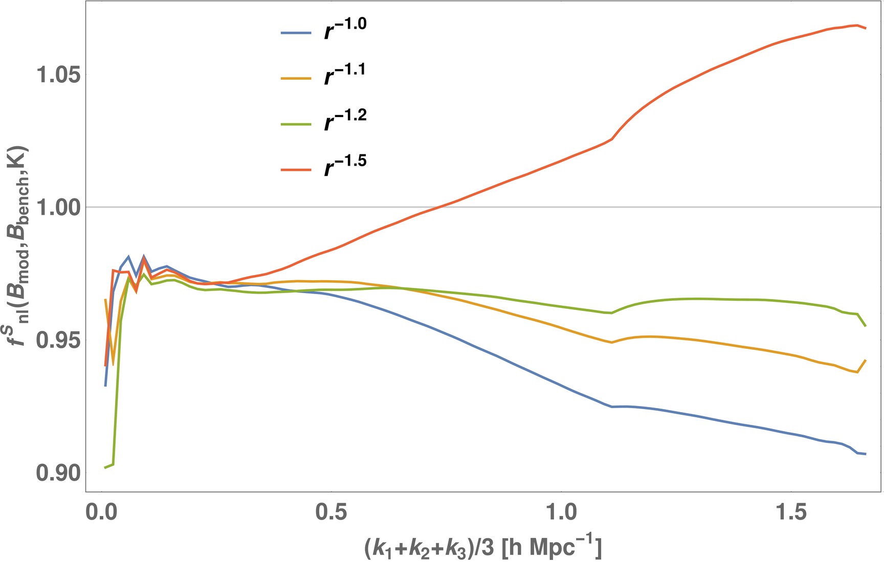
Figure IV.16: Fine-tuning the halo profile for the joint lognormal-Gaussian model to dampen the high-$k$ tail.

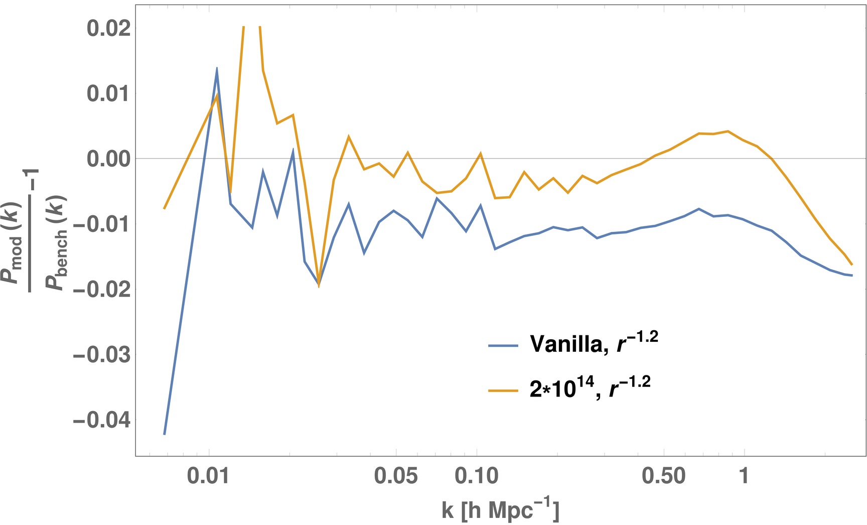
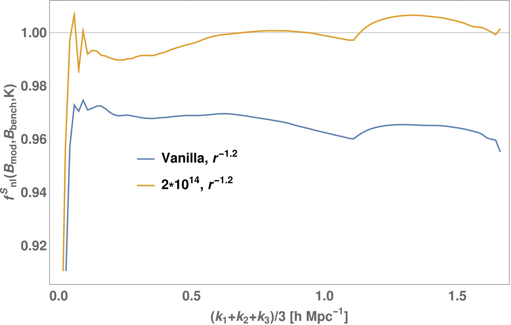
Figure IV.17: Improvements to joint lognormal-Gaussian assembly bias model by putting an extra galaxy into high mass halos (see text). The number in the labels represent the mass threshold, and ’Vanilla’ denotes the original joint lognormal-Gaussian model without alterations.

In summary, we can now implement our assembly bias model using the joint probability distribution $P(N_{g}|M,c)$ using one of four possible methods:

• For an individual halo, use the joint lognormal distribution to draw a suitable value for $N_{g}$ by shifting the Gaussian distribution for $\ln(N_{g})$ using the the concentration $c$ given for that halo by ROCKSTAR;

• Follow the same procedure as in 1 but with the joint lognormal-Gaussian, shifting the Gaussian distribution for $\ln(N_{g})$ using the individual halo concentration given by ROCKSTAR;

• Use the joint lognormal distribution for $N_{g}$ and $c$, but draw values at random for $c$ from the Gaussian distribution for $\ln(c)$, thus eliminating the need for the simulation to provide this information.

• Follow the same procedure as in 3 but with the joint lognormal-Gaussian distribution, drawing both $c$ and $N_{g}$ randomly, so the simulation again does not provide information about concentration. (For methods 3 and 4 we impose a lower bound of 2 for random draws of $c$, which is lowest value of $c$ calculated by ROCKSTAR.)

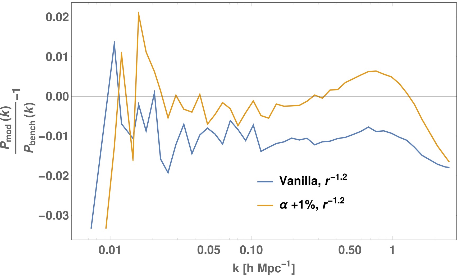
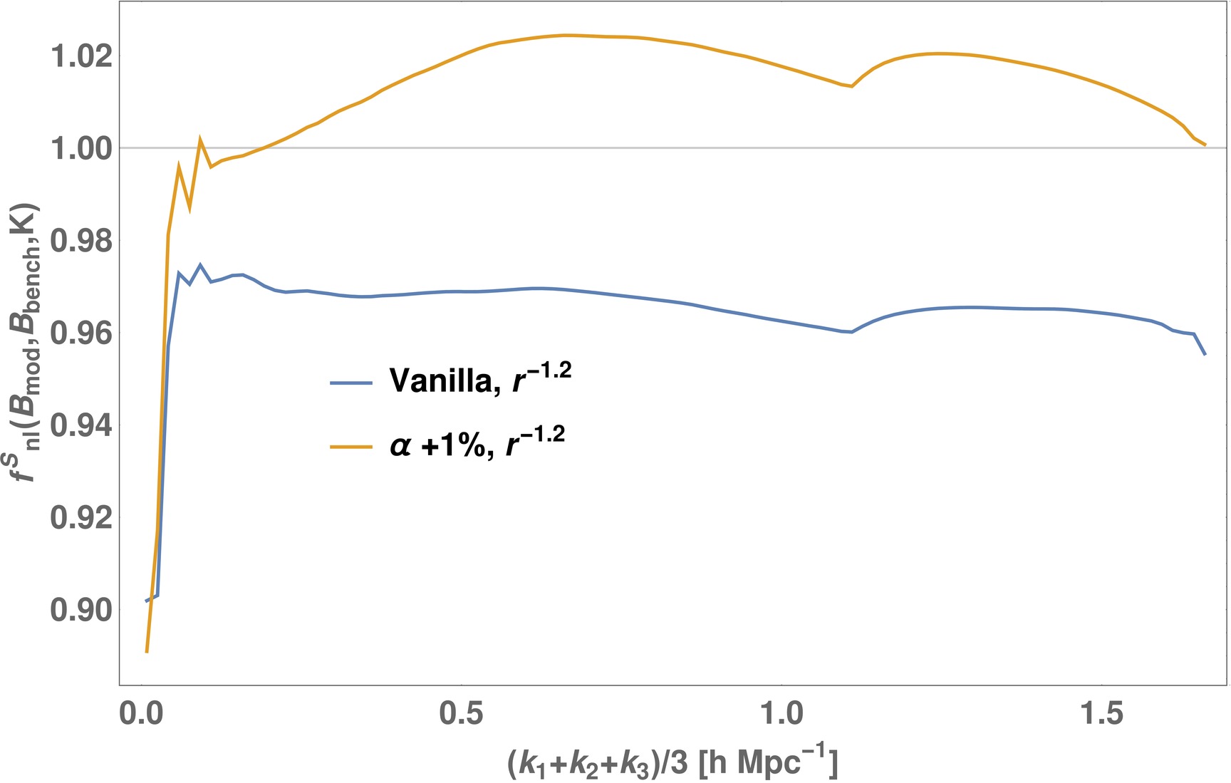
Figure IV.18: Improvements to joint lognormal-Gaussian assembly bias model by boosting $\alpha$ (see text).

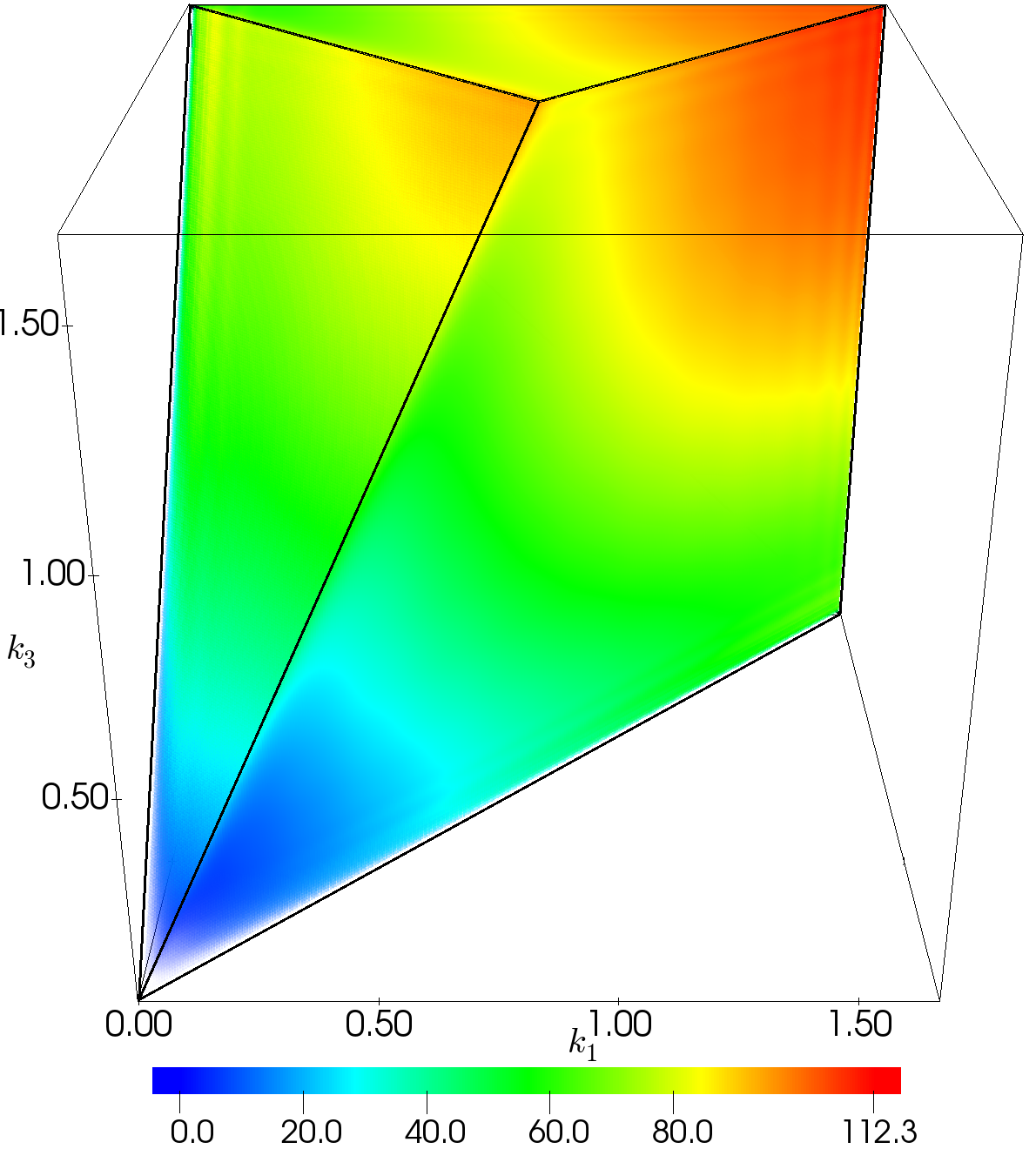
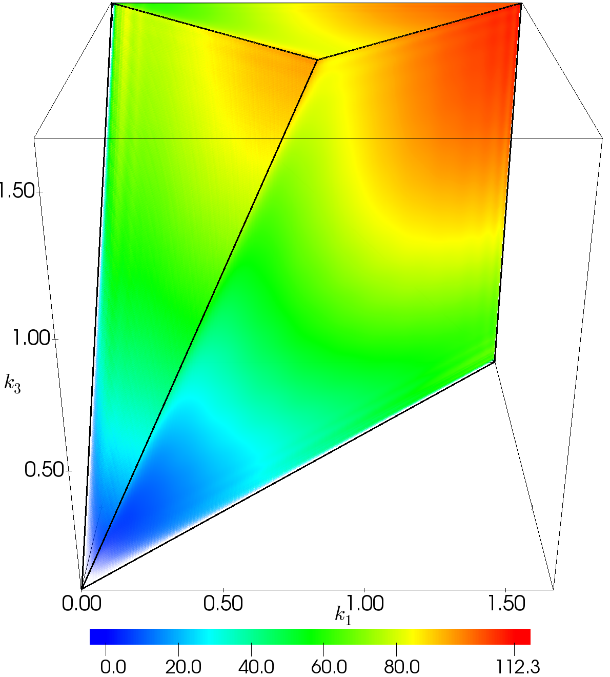
Figure IV.19: Improvements to joint lognormal-Gaussian assembly bias model. The halo profile is radial with $\gamma=1.2$. Left panel: Adding an extra galaxy to all parent halos with mass greater than $2\times 10^{13}\,h^{-1}M_{\odot}$. Right panel: Boosting $\alpha$ by 1%.

The resulting power spectra and bispectra from these prescriptions for creating mock catalogues are shown in Figure IV.15, with a comparison also to the two-bin concentration model described above. As explained in Figure III.5 the kink at $K/3=1.1\,h\,\text{Mpc}^{-1}$ is due to the geometry of the tetrapyd rather than a physical discontinuation. All these methods, endeavouring to incorporate assembly bias in some form, offer a very substantial improvement over the simplest HOD case shown in Figure II.4. Out of these four possibilities, the superior methods also exploit knowledge of individual halo concentrations given by the ROCKSTAR simulation (which to some extent also includes the simpler two-bin method described earlier). The well-motivated joint lognormal-Gaussian modelling of the occupation number and concentration, with a power law halo profile of $\gamma=1.2$, yields a better than 1% accuracy in the power spectrum and 4% accuracy in the bispectrum for $k,K/3<1.0\,h\,\text{Mpc}^{-1}$, which is significantly better than methods previously investigated in this paper. Moreover, both its power spectrum and bispectrum are flatter than the joint lognormal-lognormal case which makes it the more suitable model. It is clear that some information about the assembly history of halos is certainly helpful when creating mock catalogues targeting an accurate halo bispectrum, as it can be used a proxy for concentration. Information about the merger history of halos can be obtained by fast simulation methods without resorting to $N$-body simulations (see, for example, PINOCCHIO (Monaco et al., 2013)). A number of methods have been developed to correlate halo concentration with halo mass and redshift (Ludlow et al., 2014; Correa et al., 2015; Ludlow et al., 2016), and furthermore the authors of (Benson et al., 2019) have shown that these models, combined with an empirical model of environmental effects on halo formation times, gives the correct mean concentration and scatter as a function of halo mass.

As can be seen from Figure IV.15, there is still some room for improvement to obtain high precision mock power spectra and bispectra to match the benchmark results. In Figure IV.16 we explore changes to the halo profile for the joint lognormal-Gaussian model to curtail the excess power at small scales. It is clear that a value of $\gamma=1.2$, which is in the range of best fit values shown in Figure II.3, gives both a flat relative power spectrum and bispectrum. We also studied methods by which we might be able to generically boost the power spectrum and bispectrum across all scales, notable large length scales. From our investigations of different mass halos, we found that the high mass halos dominate the power at large scales, due to their high occupation number. One way to boost the power is therefore to add an extra galaxy to every parent halo above a certain mass threshold. We tested this tweak using the joint lognormal-Gaussian model, the results of which are shown in Figure IV.18. We found that $M=2\times 10^{14}\,h^{-1}M_{\odot}$ seems to be the appropriate mass threshold, which coupled with a radial profile of $r^{-1.2}$ allows us to obtain a fit to both the power spectrum and bispectrum to 1% accuracy between $0.04\,h\,\text{Mpc}^{-1}<k<1.1\,h\,\text{Mpc}^{-1}$. The average occupation number at this mass threshold is about 11, therefore this boost is at the 10% level in magnitude. A more natural, continuous transition, such as the $\operatorname{erfc}$ function used in the 5-parameter HOD model, can be adopted instead of a step function to obtain smoother behaviour. This may seem a rather contrived way to boost power, but it is presumably compensating some missing physical correlation (such as triaxiality etc.).

Another means by which to achieve a power boost is to raise the the power law exponent index $\alpha$ in the marginalised HOD (Equation II.12), as we did with the 4-parameter model. Instead of using the analytical form as we did previously, we change the occupation number drawn from the joint distribution by scaling the number of satellites by this factor:

$$\left(\frac{M-\kappa^{\prime}M_{0}}{M_{1}}\right)^{\alpha^{\prime}}/\left(\frac{M-\kappa M_{0}}{M_{1}}\right)^{\alpha},$$ (IV.7)

as we boost both $\alpha$ and $\kappa$ to conserve particle number. We use the best fit parameters for $\alpha$, $\kappa$, $M_{0}$ and $M_{1}$, and the results are shown in Figure IV.18. The power spectrum results are comparably to the extra galaxy method above, but this has the additional property of over-boosting the bispectrum, as we have observed in the 4-parameter HOD case. Finally, we show the 3D bispectrum tetrapyd of these improved models in Figure IV.19 which are qualitatively indistinguishable from the bispectrum obtained directly from the benchmark halo distribution.

Conclusions

In this paper we have applied the fast bispectrum estimator MODAL-LSS (Hung et al., 2019) to accurately measure the bispectrum from a large mock galaxy catalogue. This catalogue was generated from a GADGET-3 $N$-body simulation using the ROCKSTAR halo-finder. We have provided a quantitative three-shape fit to the resulting halo bispectrum, comparing it with the corresponding bispectrum of the underlying dark matter, studied previously (Lazanu et al., 2016). A key goal has been to determine phenomenological methods to create fast mock catalogues that can reproduce the benchmark halo bispectrum from ROCKSTAR. In doing so we have restricted ourselves to using only the mass, position and concentration information for parent halos, relying on statistical modelling of the halo profile and occupation number to recover the benchmark power spectrum and bispectrum. We modelled these effects in configuration space to obtain accurate mock power spectra and bispectra, and we aim to incorporate further observational effects such as RSDs in a future paper.

Halo profile

An important ingredient in a phenomenological galaxy catalogue is the spatial distribution of the galaxies within a parent halo. The subhalo radial number density found for parent halos (separated into a number of mass bins) was not well matched by the average NFW dark matter profile found in the same halo mass range. On the other hand, as suggested, e.g., by (Frenk et al., 2016) a power law profile of the form $\rho\propto r^{-\gamma}$, with $\gamma\sim 1$, works well as a universal profile across a wide range of halo masses spanning three orders of magnitude.

By randomising the solid angular distribution of the benchmark halos we have also quantified the power loss in the power spectrum and bispectrum if halo substructure and triaxiality are not preserved, that is, by fixing the original subhalo number and then retaining radial distances while randomising angular positions. The effect of this internal redistribution was modest with deviations less than 1% and 4% at $k,K/3=1\,h\,\text{Mpc}^{-1}$ for the power spectrum and bispectrum correlator respectively. These lost correlations mean that the best fit power law profile near $\gamma\approx 1$ is necessarily power deficient at small scales. However, we have found that phenomenological values around $\gamma\approx 1.5$ apparently help to recover this power loss to less than 0.5% up to $k,K/3=2\,h\,\text{Mpc}^{-1}$ in both power spectrum and bispectrum. Note that these profile modifications are constrained by using the original occupation numbers for individual halos, which is information generally only available from costly nonlinear simulations.

Halo occupation distribution

To statistically model the number of galaxies within a parent halo, we have investigated the popular practice of using an HOD that only depends on halo mass, $\bar{N}_{g}(M)$. We observed that using the measured mean number of galaxies for a halo of a given mass $M$ to repopulate the parent halos leads to a power deficit of about 2% in the power spectrum at large scales where $k<0.1\,h\,\text{Mpc}^{-1}$, and greater differences at smaller length scales. The loss of power in the bispectrum is more pronounced with much poorer scaling, yielding deviations exceeding 10% by $k=0.5\,h\,\text{Mpc}^{-1}$. We found that the same effect can be reproduced if one shuffles the given halo occupation numbers within the mass bins (or by using a dispersion around the mean HOD value). Clearly this simple HOD prescription for populating halos destroys important correlations, so it suggests that other physical mechanisms are contributing to the number of galaxies per halo, rather than just the halo mass.

Nevertheless, we have attempted to recover this power loss by tuning the four-parameter HOD model given by (Section II.3). The best fit parameters actually lead to further power loss at all scales, perhaps because the HOD fit is only accurate up to 10%, which suggests that a better functional form should be adopted to match HODs from simulations. After tweaking the parameters while keeping galaxy number constant we found that boosting the power law exponent $\alpha$ by 4.5% raised the power spectrum to the correct level to $k=0.5\,h\,\text{Mpc}^{-1}$ irrespective of choice in the other parameter, but unfortunately this results in substantially over-boosting the bispectrum (overcompensating at around the 10% level). We infer that an HOD model which only depends on halo mass cannot accurately reproduce both the power spectrum and bispectrum of a benchmark mock catalogue.

Assembly bias

These investigations led us to incorporate further information in the HOD that takes into account the formation history of the halos to determine the halo occupation number. Motivated by other assembly bias studies in the literature such as (Vakili and Hahn, 2019; Gao et al., 2005; Sunayama et al., 2016; Hearin et al., 2016; Wechsler et al., 2006), we have developed a new prescription using a joint probability distribution to model correlations between the halo occupation number $N_{g}$ and concentration $c$ found in the benchmark catalogue. Even an extension which just separates halos of a given mass into two concentration bins (Eisenstein et al., 2018) - representing above and below median values for $c$ - yields more accurate power spectra and bispectra with improved scaling.

We have found that the marginalised distribution for halo concentration is well described by a Gaussian distribution across the entire mass range of the benchmark, while taking care to impose an appropriate lower bound when drawing from the distribution. On the other hand the marginalised halo occupation number is well fitted with a lognormal distribution. Our assembly bias model is therefore a joint lognormal-Gaussian bivariate distribution which depends on halo mass, $P(N_{g}\cap c\,|M)$. A non-zero covariance between the two variables imply that halo concentration is correlated with halo occupation number, and we find the correlation coefficient is $r\approx-0.5$ for a mass range of $M=10^{13}-10^{14}h^{-1}\,M_{\odot}$. In terms of the assembly history within an $N$-body simulation, we can interpret higher halo concentration causing fewer subhalos because of earlier halo formation, that is, in this case there is more time for the merger of substructure (a factor which depends to some extent on our benchmark resolution). We were also able to obtain very similar results using a joint lognormal-lognormal distribution for the halo number and concentration.

Prescriptions for fast mock catalogue polyspectra

One of the key results of our paper is that our assembly bias model for populating halos can recover the benchmark power spectrum to within 1% and the bispectrum to within 4% across the entire range of scales of the simulation. In its most accurate form this involves using a joint lognormal-Gaussian probability distribution for $N_{g}$ and $c$, coupled with a radial power law halo profile with $\gamma=1.2$, together with the concentrations found for individual halos. Without use of individual halo concentrations, we could assign both concentration and halo number statistically, obtaining good bispectrum scaling though with a 2% and 5% deficit emerging for the power spectrum and bispectrum respectively. These assembly bias prescriptions represent a considerable improvement over all the other methods we investigated in this paper and can be deployed with fast mock catalogue generators.

We also explored ways to phenomenologically reduce this small remaining power deficit. Modifying the index in the four-parameter HOD model, as before, encountered the problem of over-boosting the bispectrum. However, motivated by the dominant contributions of high mass halos, we considered enhancing this by adding an extra galaxy to all parent halos above a certain mass threshold $M>2\times 10^{14}\,h^{-1}M_{\odot}$. We were able to obtain a 1% fit to both the benchmark power spectrum and bispectrum in the range $0.04\,h\,\text{Mpc}^{-1}<k<1.1\,h\,\text{Mpc}^{-1}$.

Finally we note a few caveats about the mock catalogue population methods we have proposed. Our assumption that galaxies can be identified with subhalos will have an important impact on both the spatial distribution and occupation number of the parent halos; clearly this approach can be developed further and made more realistic by increasing resolution and incorporating more physical mechanisms in the simulations. For example, our present mass resolution with a particle mass of $M_{p}=2.093\times 10^{10}$ may be insufficient to ensure finer substructures are resolved and preserved during halo mergers; it would be prudent in future to expand these investigations by exploring the dependence on simulation resolution. We also note that our most accurate assembly bias model relies on concentration information for individual halos obtained from the mock catalogue simulation. This is not necessarily available from all fast simulation generators and halo finder codes, but algorithms such as PINOCCHIO can provide the merger history of dark matter halos, which in turn could be converted into halo concentrations. Nevertheless, by statistically sampling the Gaussian distribution for concentration we were still able to obtain a good power spectrum and bispectrum fit, and this model can be further fine-tuned with the galaxy boost.

In summary, motivated by assembly bias, we have developed a statistical prescription for populating parent halos with subhalos which can simultaneously reproduce both the halo power spectrum and bispectrum obtained from nonlinear $N$-body simulations. We anticipate that this robust approach can be adapted to match polyspectra obtained from more sophisticated $N$-body and hydrodynamic simulations. Combining this relatively simple methodology with fast estimators like MODAL-LSS (Hung et al., 2019) should enable the bispectrum to become a key diagnostic tool, both for breaking degeneracies in cosmological parameter estimation and for quantitatively analysing gravitational collapse and other physical effects on highly nonlinear length scales.

References

- The Dark Energy Survey Collaboration (2005) The Dark Energy Survey Collaboration, “The Dark Energy Survey,” (2005), arXiv:astro-ph/0510346 .
- Diehl et al. (2014) H. T. Diehl et al., Proc.SPIE 9149 (2014), 10.1117/12.2056982.
- Ivezic et al. (2008) Z. Ivezic et al., “LSST: from Science Drivers to Reference Design and Anticipated Data Products,” (2008), arXiv:0805.2366 .
- Laureijs et al. (2011) R. Laureijs et al., “Euclid Definition Study Report,” (2011), arXiv:1110.3193 .
- Brenna Flaugher (2014) C. B. Brenna Flaugher, Proc.SPIE 9147 (2014), 10.1117/12.2057105.
- Karagiannis et al. (2018) D. Karagiannis, A. Lazanu, M. Liguori, A. Raccanelli, N. Bartolo, and L. Verde, “Constraining primordial non-gaussianity with bispectrum and power spectum from upcoming optical and radio surveys,” (2018), arXiv:1801.09280 .
- Planck Collaboration (2014) Planck Collaboration, A&A 571, A20 (2014).
- Hung et al. (2019) J. Hung, J. R. Fergusson, and E. P. S. Shellard, “Advancing the matter bispectrum estimation of large-scale structure: a comparison of dark matter codes,” (2019), arXiv:1902.01830 .
- Wagner et al. (2010) C. Wagner, L. Verde, and L. Boubekeur, Journal of Cosmology and Astroparticle Physics 2010, 022 (2010).
- Regan et al. (2012) D. M. Regan, M. M. Schmittfull, E. P. S. Shellard, and J. R. Fergusson, Phys. Rev. D 86, 123524 (2012).
- Gil-Marín et al. (2012) H. Gil-Marín, C. Wagner, F. Fragkoudi, R. Jimenez, and L. Verde, Journal of Cosmology and Astroparticle Physics 2012, 047 (2012).
- Schmittfull et al. (2013) M. M. Schmittfull, D. M. Regan, and E. P. S. Shellard, Phys. Rev. D 88, 063512 (2013).
- Lazanu et al. (2016) A. Lazanu, T. Giannantonio, M. Schmittfull, and E. P. S. Shellard, Phys. Rev. D 93, 083517 (2016).
- Eisenstein et al. (2011) D. J. Eisenstein et al., The Astronomical Journal 142, 72 (2011).
- Dawson et al. (2013) K. S. Dawson et al., The Astronomical Journal 145, 10 (2013).
- Gil-Marín et al. (2015a) H. Gil-Marín, J. Noreña, L. Verde, W. J. Percival, C. Wagner, M. Manera, and D. P. Schneider, Monthly Notices of the Royal Astronomical Society 451, 539 (2015a).
- Gil-Marín et al. (2015b) H. Gil-Marín, L. Verde, J. Noreña, A. J. Cuesta, L. Samushia, W. J. Percival, C. Wagner, M. Manera, and D. P. Schneider, Monthly Notices of the Royal Astronomical Society 452, 1914 (2015b).
- Gil-Marín et al. (2017) H. Gil-Marín et al., Monthly Notices of the Royal Astronomical Society 465, 1757 (2017).
- Howlett et al. (2015) C. Howlett, M. Manera, and W. J. Percival, “L-PICOLA: A parallel code for fast dark matter simulation,” (2015), arXiv:1506.03737 .
- Gualdi et al. (2019a) D. Gualdi, H. Gil-Marín, M. Manera, B. Joachimi, and O. Lahav, Monthly Notices of the Royal Astronomical Society: Letters 484, L29 (2019a), http://oup.prod.sis.lan/mnrasl/article-pdf/484/1/L29/27496796/sly242.pdf .
- Gualdi et al. (2018) D. Gualdi, M. Manera, B. Joachimi, and O. Lahav, Monthly Notices of the Royal Astronomical Society 476, 4045 (2018), http://oup.prod.sis.lan/mnras/article-pdf/476/3/4045/24541764/sty261.pdf .
- Gualdi et al. (2019b) D. Gualdi, H. Gil-Marín, R. L. Schuhmann, M. Manera, B. Joachimi, and O. Lahav, Monthly Notices of the Royal Astronomical Society 484, 3713 (2019b), http://oup.prod.sis.lan/mnras/article-pdf/484/3/3713/27723669/stz051.pdf .
- Heavens et al. (2017) A. F. Heavens, E. Sellentin, D. de Mijolla, and A. Vianello, Monthly Notices of the Royal Astronomical Society 472, 4244 (2017), arXiv:1707.06529 [astro-ph.CO] .
- Alsing and Wandelt (2018) J. Alsing and B. Wandelt, Monthly Notices of the Royal Astronomical Society: Letters 476, L60 (2018), http://oup.prod.sis.lan/mnrasl/article-pdf/476/1/L60/24566044/sly029.pdf .
- Kaiser (1984) N. Kaiser, The Astrophysical Journal 284, L9 (1984).
- Gelb and Bertschinger (1994) J. M. Gelb and E. Bertschinger, The Astrophysical Journal 436, 467 (1994), astro-ph/9408028 .
- Klypin and Holtzman (1997) A. Klypin and J. Holtzman, “Particle-mesh code for cosmological simulations,” (1997), arXiv:astro-ph/9712217 .
- Eisenstein and Hut (1998) D. J. Eisenstein and P. Hut, The Astrophysical Journal 498, 137 (1998), astro-ph/9712200 .
- Bullock et al. (2001) J. S. Bullock, T. S. Kolatt, Y. Sigad, R. S. Somerville, A. V. Kravtsov, A. A. Klypin, J. R. Primack, and A. Dekel, Monthly Notices of the Royal Astronomical Society 321, 559 (2001), astro-ph/9908159 .
- Springel et al. (2001) V. Springel, S. D. M. White, G. Tormen, and G. Kauffmann, Monthly Notices of the Royal Astronomical Society 328, 726 (2001).
- Stadel (2001) J. G. Stadel, Cosmological N-body simulations and their analysis, Ph.D. thesis, UNIVERSITY OF WASHINGTON (2001).
- Aubert et al. (2004) D. Aubert, C. Pichon, and S. Colombi, Monthly Notices of the Royal Astronomical Society 352, 376 (2004), astro-ph/0402405 .
- Gill et al. (2004) S. P. D. Gill, A. Knebe, and B. K. Gibson, Monthly Notices of the Royal Astronomical Society 351, 399 (2004), astro-ph/0404258 .
- Neyrinck et al. (2005) M. C. Neyrinck, N. Y. Gnedin, and A. J. S. Hamilton, Monthly Notices of the Royal Astronomical Society 356, 1222 (2005), astro-ph/0402346 .
- Weller et al. (2005) J. Weller, J. P. Ostriker, P. Bode, and L. Shaw, Monthly Notices of the Royal Astronomical Society 364, 823 (2005), astro-ph/0405445 .
- Diemand et al. (2006) J. Diemand, M. Kuhlen, and P. Madau, The Astrophysical Journal 649, 1 (2006), astro-ph/0603250 .
- Kim and Park (2006) J. Kim and C. Park, The Astrophysical Journal 639, 600 (2006), astro-ph/0401386 .
- Gardner et al. (2007) J. P. Gardner, A. Connolly, and C. McBride, in Proceedings of the 5th IEEE Workshop on Challenges of Large Applications in Distributed Environments, CLADE ’07 (ACM, New York, NY, USA, 2007) pp. 1–10.
- Shaw et al. (2007) L. D. Shaw, J. Weller, J. P. Ostriker, and P. Bode, The Astrophysical Journal 659, 1082 (2007), astro-ph/0603150 .
- Habib et al. (2009) S. Habib, A. Pope, Z. Lukić, D. Daniel, P. Fasel, N. Desai, K. Heitmann, C.-H. Hsu, L. Ankeny, G. Mark, S. Bhattacharya, and J. Ahrens, in Journal of Physics Conference Series, Journal of Physics Conference Series, Vol. 180 (2009) p. 012019.
- Knollmann and Knebe (2009) S. R. Knollmann and A. Knebe, The Astrophysical Journal Supplement 182, 608 (2009), arXiv:0904.3662 .
- Maciejewski et al. (2009) M. Maciejewski, S. Colombi, V. Springel, C. Alard, and F. R. Bouchet, Monthly Notices of the Royal Astronomical Society 396, 1329 (2009), arXiv:0812.0288 .
- Ascasibar (2010) Y. Ascasibar, Computer Physics Communications 181, 1438 (2010).
- Behroozi et al. (2013) P. S. Behroozi, R. H. Wechsler, and H.-Y. Wu, The Astrophysical Journal 762, 109 (2013).
- Planelles and Quilis (2010) S. Planelles and V. Quilis, Astronomy and Astrophysics 519, A94 (2010), arXiv:1006.3205 .
- Rasera et al. (2010) Y. Rasera, J.-M. Alimi, J. Courtin, F. Roy, P.-S. Corasaniti, A. Füzfa, and V. Boucher, in American Institute of Physics Conference Series, American Institute of Physics Conference Series, Vol. 1241, edited by J.-M. Alimi and A. Fuözfa (2010) pp. 1134–1139, arXiv:1002.4950 .
- Skory et al. (2010) S. Skory, M. J. Turk, M. L. Norman, and A. L. Coil, The Astrophysical Journal Supplement 191, 43 (2010), arXiv:1001.3411 .
- Sutter and Ricker (2010) P. M. Sutter and P. M. Ricker, The Astrophysical Journal 723, 1308 (2010), arXiv:1006.2879 [astro-ph.CO] .
- Falck et al. (2012) B. L. Falck, M. C. Neyrinck, and A. S. Szalay, The Astrophysical Journal 754, 126 (2012).
- Wu et al. (2010) H.-Y. Wu, A. R. Zentner, and R. H. Wechsler, The Astrophysical Journal 713, 856 (2010), arXiv:0910.3668 .
- Cunha and Evrard (2010) C. E. Cunha and A. E. Evrard, Physical Review D 81, 083509 (2010), arXiv:0908.0526 [astro-ph.CO] .
- Davis et al. (1985) M. Davis, G. Efstathiou, C. S. Frenk, and S. D. M. White, The Astrophysical Journal 292, 371 (1985).
- Press and Schechter (1974) W. H. Press and P. Schechter, The Astrophysical Journal 187, 425 (1974).
- Knebe et al. (2011) A. Knebe, S. R. Knollmann, S. I. Muldrew, F. R. Pearce, M. A. Aragon-Calvo, Y. Ascasibar, P. S. Behroozi, D. Ceverino, S. Colombi, J. Diemand, K. Dolag, B. L. Falck, P. Fasel, J. Gardner, S. Gottlöber, C.-H. Hsu, F. Iannuzzi, A. Klypin, Z. Lukić, M. Maciejewski, C. McBride, M. C. Neyrinck, S. Planelles, D. Potter, V. Quilis, Y. Rasera, J. I. Read, P. M. Ricker, F. Roy, V. Springel, J. Stadel, G. Stinson, P. M. Sutter, V. Turchaninov, D. Tweed, G. Yepes, and M. Zemp, Monthly Notices of the Royal Astronomical Society 415, 2293 (2011), http://oup.prod.sis.lan/mnras/article-pdf/415/3/2293/5972749/mnras0415-2293.pdf .
- Planck Collaboration (2016) Planck Collaboration, Astronomy & Astrophysics 594, A13 (2016).
- McCullagh et al. (2016) N. McCullagh, D. Jeong, and A. S. Szalay, Monthly Notices of the Royal Astronomical Society 455, 2945 (2016).
- Crocce et al. (2006) M. Crocce, S. Pueblas, and R. Scoccimarro, Monthly Notices of the Royal Astronomical Society 373, 369 (2006).
- Scoccimarro et al. (2012) R. Scoccimarro, L. Hui, M. Manera, and K. C. Chan, Phys. Rev. D 85, 083002 (2012).
- Lewis et al. (2000) A. Lewis, A. Challinor, and A. Lasenby, The Astrophysical Journal 538, 473 (2000).
- Eisenstein et al. (2017) D. J. Eisenstein, L. H. Garrison, and S. Yuan, Monthly Notices of the Royal Astronomical Society 472, 577 (2017).
- Eisenstein et al. (2018) D. J. Eisenstein, L. H. Garrison, and S. Yuan, Monthly Notices of the Royal Astronomical Society 478, 2019 (2018).
- Padmanabhan et al. (2007) N. Padmanabhan, D. J. Schlegel, U. Seljak, A. Makarov, N. A. Bahcall, M. R. Blanton, J. Brinkmann, D. J. Eisenstein, D. P. Finkbeiner, J. E. Gunn, D. W. Hogg, Ž. Ivezić, G. R. Knapp, J. Loveday, R. H. Lupton, R. C. Nichol, D. P. Schneider, M. A. Strauss, M. Tegmark, and D. G. York, Monthly Notices of the Royal Astronomical Society 378, 852 (2007), astro-ph/0605302 .
- Scoccimarro (2000) R. Scoccimarro, The Astrophysical Journal 544, 597 (2000).
- Manera et al. (2013) M. Manera, R. Scoccimarro, W. J. Percival, L. Samushia, C. K. McBride, A. J. Ross, R. K. Sheth, M. White, B. A. Reid, A. G. Sánchez, R. de Putter, X. Xu, A. A. Berlind, J. Brinkmann, C. Maraston, B. Nichol, F. Montesano, N. Padmanabhan, R. A. Skibba, R. Tojeiro, and B. A. Weaver, Monthly Notices of the Royal Astronomical Society 428, 1036 (2013), arXiv:1203.6609 .
- Kitaura et al. (2016) F.-S. Kitaura, S. Rodríguez-Torres, C.-H. Chuang, C. Zhao, F. Prada, H. Gil-Marín, H. Guo, G. Yepes, A. Klypin, C. G. Scóccola, J. Tinker, C. McBride, B. Reid, A. G. Sánchez, S. Salazar-Albornoz, J. N. Grieb, M. Vargas-Magana, A. J. Cuesta, M. Neyrinck, F. Beutler, J. Comparat, W. J. Percival, and A. Ross, Monthly Notices of the Royal Astronomical Society 456, 4156 (2016), arXiv:1509.06400 .
- Vega-Ferrero et al. (2017) J. Vega-Ferrero, G. Yepes, and S. Gottlöber, Monthly Notices of the Royal Astronomical Society 467, 3226 (2017), http://oup.prod.sis.lan/mnras/article-pdf/467/3/3226/10875743/stx282.pdf .
- Schneider et al. (2012) M. D. Schneider, C. S. Frenk, and S. Cole, Journal of Cosmology and Astroparticle Physics 2012, 030 (2012).
- Vera-Ciro et al. (2011) C. A. Vera-Ciro, L. V. Sales, A. Helmi, C. S. Frenk, J. F. Navarro, V. Springel, M. Vogelsberger, and S. D. M. White, Monthly Notices of the Royal Astronomical Society 416, 1377 (2011), http://oup.prod.sis.lan/mnras/article-pdf/416/2/1377/18594489/mnras0416-1377.pdf .
- Angrick, C. and Bartelmann, M. (2010) Angrick, C. and Bartelmann, M., Astronomy & Astrophysics 518, A38 (2010).
- Navarro et al. (1996) J. F. Navarro, C. S. Frenk, and S. D. M. White, The Astrophysical Journal 462, 563 (1996), astro-ph/9508025 .
- Bryan and Norman (1998) G. L. Bryan and M. L. Norman, The Astrophysical Journal 495, 80 (1998), astro-ph/9710107 .
- Cooray and Sheth (2002) A. Cooray and R. Sheth, Physics Reports 372, 1 (2002).
- Klypin et al. (2011) A. A. Klypin, S. Trujillo-Gomez, and J. Primack, The Astrophysical Journal 740, 102 (2011).
- Jenkins et al. (2004) A. Jenkins, G. De Lucia, S. D. M. White, and L. Gao, Monthly Notices of the Royal Astronomical Society 352, L1 (2004).
- Libeskind et al. (2005) N. I. Libeskind, C. S. Frenk, S. Cole, J. C. Helly, A. Jenkins, J. F. Navarro, and C. Power, Monthly Notices of the Royal Astronomical Society 363, 146 (2005).
- Moore et al. (2004) B. Moore, J. Stadel, and J. Diemand, Monthly Notices of the Royal Astronomical Society 352, 535 (2004).
- Gao et al. (2004) L. Gao, S. D. M. White, A. Jenkins, F. Stoehr, and V. Springel, Monthly Notices of the Royal Astronomical Society 355, 819 (2004).
- Frenk et al. (2016) C. S. Frenk, J. Han, S. Cole, and Y. Jing, Monthly Notices of the Royal Astronomical Society 457, 1208 (2016), http://oup.prod.sis.lan/mnras/article-pdf/457/2/1208/2882862/stv2900.pdf .
- Peacock and Smith (2000) J. A. Peacock and R. E. Smith, Monthly Notices of the Royal Astronomical Society 318, 1144 (2000), astro-ph/0005010 .
- Scoccimarro et al. (2001) R. Scoccimarro, R. K. Sheth, L. Hui, and B. Jain, The Astrophysical Journal 546, 20 (2001), astro-ph/0006319 .
- Berlind and Weinberg (2002) A. A. Berlind and D. H. Weinberg, The Astrophysical Journal 575, 587 (2002), astro-ph/0109001 .
- Zheng et al. (2009) Z. Zheng, I. Zehavi, D. J. Eisenstein, D. H. Weinberg, and Y. P. Jing, The Astrophysical Journal 707, 554 (2009).
- Anderson et al. (2014) L. Anderson, É. Aubourg, S. Bailey, F. Beutler, V. Bhardwaj, M. Blanton, A. S. Bolton, J. Brinkmann, J. R. Brownstein, A. Burden, C.-H. Chuang, A. J. Cuesta, K. S. Dawson, D. J. Eisenstein, S. Escoffier, J. E. Gunn, H. Guo, S. Ho, K. Honscheid, C. Howlett, D. Kirkby, R. H. Lupton, M. Manera, C. Maraston, C. K. McBride, O. Mena, F. Montesano, R. C. Nichol, S. E. Nuza, M. D. Olmstead, N. Padmanabhan, N. Palanque-Delabrouille, J. Parejko, W. J. Percival, P. Petitjean, F. Prada, A. M. Price-Whelan, B. Reid, N. A. Roe, A. J. Ross, N. P. Ross, C. G. Sabiu, S. Saito, L. Samushia, A. G. Sánchez, D. J. Schlegel, D. P. Schneider, C. G. Scoccola, H.-J. Seo, R. A. Skibba, M. A. Strauss, M. E. C. Swanson, D. Thomas, J. L. Tinker, R. Tojeiro, M. V. Magaña, L. Verde, D. A. Wake, B. A. Weaver, D. H. Weinberg, M. White, X. Xu, C. Yèche, I. Zehavi, and G.-B. Zhao, Monthly Notices of the Royal Astronomical Society 441, 24 (2014), arXiv:1312.4877 .
- Gottlöber et al. (1999) S. Gottlöber, A. A. Klypin, and A. V. Kravtsov, in Observational Cosmology: The Development of Galaxy Systems, Astronomical Society of the Pacific Conference Series, Vol. 176, edited by G. Giuricin, M. Mezzetti, and P. Salucci (1999) p. 418, arXiv:astro-ph/9810445 [astro-ph] .
- Kravtsov and Klypin (1999) A. V. Kravtsov and A. A. Klypin, The Astrophysical Journal 520, 437 (1999).
- Mann et al. (1998) R. G. Mann, J. A. Peacock, and A. F. Heavens, Monthly Notices of the Royal Astronomical Society 293, 209 (1998), http://oup.prod.sis.lan/mnras/article-pdf/293/3/209/3881609/293-3-209.pdf .
- Ahrens et al. (2005) J. Ahrens, B. Geveci, and C. Law, ParaView: An End-User Tool for Large Data Visualization. (Visualization Handbook, Elsevier, 2005).
- Seery et al. (2017) D. Seery, R. E. Smith, A. Eggemeier, D. Regan, and J. Byun, Monthly Notices of the Royal Astronomical Society 471, 1581 (2017), http://oup.prod.sis.lan/mnras/article-pdf/471/2/1581/19407307/stx1681.pdf .
- Lazanu et al. (2017) A. Lazanu, T. Giannantonio, M. Schmittfull, and E. P. S. Shellard, Phys. Rev. D 95, 083511 (2017).
- Bouchet et al. (1995) F. R. Bouchet, S. Colombi, E. Hivon, and R. Juszkiewicz, A & A 296, 575 (1995), astro-ph/9406013 .
- Desjacques et al. (2018) V. Desjacques, D. Jeong, and F. Schmidt, Physics Reports 733, 1 (2018), large-scale galaxy bias.
- Pace et al. (2015) F. Pace, M. Manera, D. J. Bacon, R. Crittenden, and W. J. Percival, Monthly Notices of the Royal Astronomical Society 454, 708 (2015), http://oup.prod.sis.lan/mnras/article-pdf/454/1/708/3938653/stv2019.pdf .
- Smith et al. (2008) R. E. Smith, R. K. Sheth, and R. Scoccimarro, Phys. Rev. D 78, 023523 (2008).
- Vakili and Hahn (2019) M. Vakili and C. Hahn, The Astrophysical Journal 872, 115 (2019).
- Gao et al. (2005) L. Gao, V. Springel, and S. D. M. White, Monthly Notices of the Royal Astronomical Society 363, L66 (2005), astro-ph/0506510 .
- Sunayama et al. (2016) T. Sunayama, A. P. Hearin, N. Padmanabhan, and A. Leauthaud, Monthly Notices of the Royal Astronomical Society 458, 1510 (2016), arXiv:1509.06417 .
- Hearin et al. (2016) A. P. Hearin, A. R. Zentner, F. C. van den Bosch, D. Campbell, and E. Tollerud, Monthly Notices of the Royal Astronomical Society 460, 2552 (2016), arXiv:1512.03050 .
- Wechsler et al. (2006) R. H. Wechsler, A. R. Zentner, J. S. Bullock, A. V. Kravtsov, and B. Allgood, The Astrophysical Journal 652, 71 (2006).
- Zhao et al. (2003) D. H. Zhao, H. J. Mo, Y. P. Jing, and G. Börner, Monthly Notices of the Royal Astronomical Society 339, 12 (2003), astro-ph/0204108 .
- Zhao et al. (2009) D. H. Zhao, Y. P. Jing, H. J. Mo, and G. Börner, The Astrophysical Journal 707, 354 (2009), arXiv:0811.0828 .
- Villarreal et al. (2017) A. S. Villarreal, A. R. Zentner, Y.-Y. Mao, C. W. Purcell, F. C. van den Bosch, B. Diemer, J. U. Lange, K. Wang, and D. Campbell, Monthly Notices of the Royal Astronomical Society 472, 1088 (2017), arXiv:1705.04327 .
- Wechsler et al. (2002) R. H. Wechsler, J. S. Bullock, J. R. Primack, A. V. Kravtsov, and A. Dekel, The Astrophysical Journal 568, 52 (2002).
- Mao et al. (2017) Y.-Y. Mao, A. R. Zentner, and R. H. Wechsler, Monthly Notices of the Royal Astronomical Society 474, 5143 (2017), http://oup.prod.sis.lan/mnras/article-pdf/474/4/5143/23126779/stx3111.pdf .
- Stewart et al. (2009) K. R. Stewart, J. S. Bullock, E. J. Barton, and R. H. Wechsler, The Astrophysical Journal 702, 1005 (2009).
- Bayes and Price (1763) M. Bayes and M. Price, Philosophical Transactions 53, 370 (1763).
- Eaton (1983) M. L. Eaton, Multivariate statistics : a vector space approach, Wiley series in probability and mathematical statistics (Wiley, New York ; Chichester, 1983).
- Monaco et al. (2013) P. Monaco, E. Sefusatti, S. Borgani, M. Crocce, P. Fosalba, R. K. Sheth, and T. Theuns, Monthly Notices of the Royal Astronomical Society 433, 2389 (2013), http://oup.prod.sis.lan/mnras/article-pdf/433/3/2389/4061631/stt907.pdf .
- Ludlow et al. (2014) A. D. Ludlow, J. F. Navarro, R. E. Angulo, M. Boylan-Kolchin, V. Springel, C. Frenk, and S. D. M. White, Monthly Notices of the Royal Astronomical Society 441, 378 (2014), http://oup.prod.sis.lan/mnras/article-pdf/441/1/378/2996980/stu483.pdf .
- Correa et al. (2015) C. A. Correa, J. S. B. Wyithe, J. Schaye, and A. R. Duffy, Monthly Notices of the Royal Astronomical Society 452, 1217 (2015), http://oup.prod.sis.lan/mnras/article-pdf/452/2/1217/18505290/stv1363.pdf .
- Ludlow et al. (2016) A. D. Ludlow, S. Bose, R. E. Angulo, L. Wang, W. A. Hellwing, J. F. Navarro, S. Cole, and C. S. Frenk, Monthly Notices of the Royal Astronomical Society 460, 1214 (2016), http://oup.prod.sis.lan/mnras/article-pdf/460/2/1214/8115724/stw1046.pdf .
- Benson et al. (2019) A. J. Benson, A. Ludlow, and S. Cole, Monthly Notices of the Royal Astronomical Society 485, 5010 (2019), http://oup.prod.sis.lan/mnras/article-pdf/485/4/5010/28249774/stz695.pdf .