Optimal steering of a smart active particle

Abstract

We formulate the theory for steering an active particle with optimal travel time between two locations and apply it to the Mexican hat potential without brim. For small heights the particle can cross the potential barrier, while for large heights it has to move around it. Thermal fluctuations in the orientation strongly affect the path over the barrier. Then we consider a smart active particle and apply reinforcement learning. We show how the active particle learns in repeating episodes to move optimally. The optimal steering is stored in the optimized action-value function, which is able to rectify thermal fluctuations.

1 Introduction

Active motion, its understanding, and its phenomenology has evolved as a new paradigm in non-equilibrium physics as documented by recent reviews [1, 2, 3, 4, 5, 6]. The control of active motion comes more and more into focus. In particular, the motion of active particles and microswimmers is influenced by external fields, as exemplified by a few works on magnetic [7, 8], gravitational [9, 10, 11, 12, 13, 14, 15, 16, 17], and flow fields [18, 19, 20, 21, 22, 23, 24, 25]. Active particles interact through chemical fields, which they produce themselves [26, 27, 28, 29, 30, 31, 32, 33]. Other articles stress the role of boundaries [34, 35, 36], the influence of a complex environment [37, 38, 39, 6, 40], and rectified motion by active ratchets [41, 42, 43, 44, 45].

Most recent articles describe the targeted manipulation of active motion. They actively steer Janus colloids by electric fields [46], control the motion of Janus colloids with quorum sensing rules [47], design interactions by information flow between active particles [48], or describe the light-controlled assembly of active colloidal molecules [49]. How optimal search strategies depend on environment is explored in Ref. [50], while Ref. [51] suggests minimal navigation strategies for active particles [51]. In Ref. [52] Liebchen and Löwen lay the ground for optimally steering active particles on trajectories with shortest travel time. This gives a strong link to optimal control theory [53], which has been applied to viscous flow [54], to particle steering in inertial microfluidics [55], and to finance [56].

A very attractive and promising field is the application of machine or reinforcement learning to active motion. A comprehensive account of reinforcement learning is found in Ref. [57]. Self-propelled entities learn in repeating episodes to perform a prescribed task. This includes a glider, which learns to soar in turbulent environments [58], flow navigation of smart microswimmers under gravity [59], and their navigation in a grid world [60].

This article addresses the optimal steering of active particles in a prescribed potential landscape. We first formulate the theory for optimizing the travel time of an active particle, the orientation of which can be controlled in order to steer it between two locations. An example are magnetotactic bacteria, which align along an external magnetic field [7]. We apply the formalism to the Mexican hat potential without brim. For small barrier heights the active particle crosses the potential barrier on a straight path, while for large heights it has to move around it. We demonstrate how volatile the optimal path is to thermal fluctuations in the prescribed orientation when crossing the barrier. We then make the active particle smart and apply reinforcement learning. We demonstrate how the active particle learns in repeating episodes to move on the optimal path by storing its knowledge in the optimized action-value function. Now, fluctuations in the prescribed orientation are rectified by this optimized function.

2 Optimal steering

We consider an active particle that moves with swimming speed $v_{0}$ along an intrinsic direction given by unit vector $\bm{e}$ and under the influence of a potential force $\bm{F}=-\nabla U$. Its total velocity is $\bm{v}=v_{0}\bm{e}+\bm{F}/\xi$, where $\xi$ is the friction coefficient, and we neglect any thermal noise for the moment. We assume the orientation $\bm{e}$ of the particle can be controlled and then search for the trajectory with the optimal travel time $T$ (fastest trajectory), when the particle is steered from initial position $\bm{r}_{i}$ to final position $\bm{r}_{f}$,

$$T=\int_{\bm{r}_{i}}^{\bm{r}_{f}}dt=\int_{\bm{r}_{i}}^{\bm{r}_{f}}\frac{ds}{v}\,.$$ (1)

In the following we use unitless quantities by replacing $\bm{v}/v_{0}\rightarrow\bm{v}$, $\bm{F}/\xi v_{0}\rightarrow\bm{F}$, and $\bm{r}/L\rightarrow\bm{r}$, where $L$ is a characteristig length. The total velocity then becomes

$$\bm{v}=\bm{e}+\bm{F}\,.$$ (2)

Parametrizing the trajectory $\bm{r}(s)$ with the arc length $s$, we can write the unit tangent along the trajectory and the total active-particle velocity as

$$\bm{t}=\frac{d\bm{r}}{ds}\quad\text{and}\quad\bm{v}=v\bm{t}\,,$$ (3)

respectively. From the square of $\bm{v}$ from Eq. (2) and replacing $\bm{e}$ by $v\bm{t}-\bm{F}$, we obtain a quadratic polynomial for the total active-particle speed $v$. We determine the zero and arrive at an expression for the particle speed,

$$v=\bm{t}\cdot\bm{F}+\sqrt{1-[\bm{F}^{2}-(\bm{t}\cdot\bm{F})^{2}]}\,.$$ (4)

For $\bm{F}=\bm{0}$ we correctly obtain $v=1$, while the second zero would give $v=-1$. The term in the square brackets on the right-hand side denotes the square of the force component perpendicular to $\bm{t}$.

Now, the variation of the travel time, $\delta T=0$, using Eq. (4) in Eq. (1) determines the fastest trajectory in an arbitrary potential force field. To mimimize $T$ for a two-dimensional trajectory in the $xy$ plane, we write the trajectory as $y=y(x)$ and discretize the travel time, where $ds=\sqrt{1+[y^{\prime}(x)]^{2}}dx$. Starting from initial trajectories, we mimimize $T$ based on the routine fminunc in the program MATLAB.

3 Fastest trajectories

3.1 Mexican hat potential without brim

To illustrate the optimization of the travel time, we look at active motion in two dimensions in a radially symmetric potential with a potential barrier taken from the Mexican hat potential, while outside the minimum the potential is zero:

$$U=\left\{\begin{array}[]{l}16U_{0}(\rho^{2}-1/4)^{2}\enspace,\enspace\rho\leq 1/2\\ 0\end{array}\right.\,,$$ (5)

where $\rho$ is the radial distance from the center. The potential has a barrier at $\rho=0$ with height $U_{0}$ and a ring of minima at $\rho=1/2$. The maximum potential force at the ring of inflection points at $\rho=1/2\sqrt{3}$ is $F_{\text{max}}\bm{e}_{\rho}=-\partial U/\partial\rho\bm{e}_{\rho}=16U_{0}/3\sqrt{3}\bm{e}_{\rho}$. Figure 1a) shows the color-coded potential.

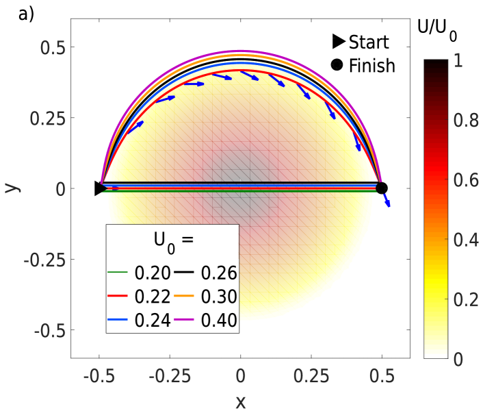
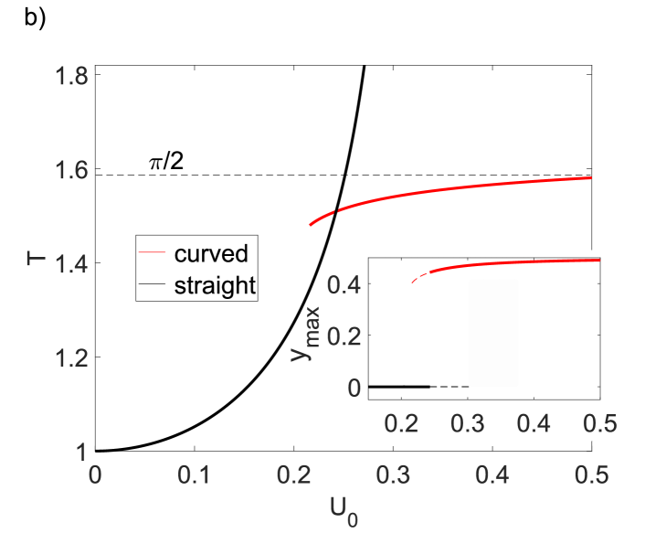
Figure 1: a) Optimal trajectories of an active particle in a Mexican hat potential without brim (color-coded) for different $U_{0}$. Trajectories with a local minimum in $T$ are shown starting at $x=-0.5$ and ending at $0.5$. For $U_{0}=0.22$ the particle orientations $\bm{e}$ along the trajectory are indicated. b) Travel time $T$ plotted versus $U_{0}$ for straight and curved trajectories. For the curved trajectory $T\rightarrow\pi/2$ for $U_{0}\rightarrow\infty$. Inset: Maximum displacement $y_{\text{max}}$ versus $U_{0}$. Solid and dashed lines mean absolute and metastable minima of $T$, respectively.

We now ask what is the optimal trajectory starting on the $x$ axis at $-1/2$ and ending there at $1/2$. For small height $U_{0}$ the active particle will move on a straight path. However, with increasing $U_{0}$ it is more favorable for the active particle to move around the potential barrier. Ultimately, when the active motion ($v_{0}$) cannot overcome the maximal drift motion $F_{\text{max}}/\gamma$ induced by the potential, which in our reduced units reads $F_{\text{max}}=1$, the travel time of the straight path diverges at $U_{0}=3\sqrt{3}/16\approx 0.325$. In Fig. 1a) we demonstrate optimal trajectories that evolved either from the straight or a curved initial trajectory for different heights $U_{0}$. For $U_{0}=0.22$ we also show the local orientation $\bm{e}$. Interestingly, in the interval $U_{0}\in[0.216,0.302]$ the travel times of both trajectories are local minima. In the inset of Fig. 1b) we plot the maximal displacement in $y$ direction, $y_{\text{max}}$, for the local minima. Solid and dashed lines mean absolute and metastable minima, respectively. From the main plot in Fig. 1b) the stable minima become clear. The curved trajectory is the fastests trajectory starting from $U_{0}=0.24$ and approaches $T=\pi/2$ for $U_{0}\rightarrow\infty$, where the active particle moves in a half circle with radius $\rho=1/2$ around the barrier.

3.2 More complex potential

Of course, our method also provides optimal paths in more complex potential landscapes. As an example we take the peaks potential provided by MATLAB,

$$U_{\text{peaks}} = 0.3(1-x)^{2}\exp[-x^{2}-(y+1)^{2}]$$ (6)

$$-(0.2x-x^{3}-y^{5})\exp(-x^{2}-y^{2})$$

$$-1/30\exp[-(x+1)^{2}-y^{2}]\,,$$

which we show color-coded in Fig. 2. The different trajectories with locally minimum travel time evolved from different starting trajectories. Choosing them properly is crucial for finding the globally optimal trajectory. Here, reinforcement learning can help since it provides a means to find this trajectory.

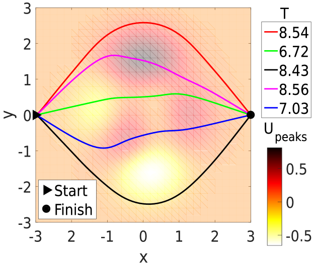
Figure 2: Locally optimal trajectories in the landscape of the peaks potential $U_{\text{peaks}}$ of MATLAB. The trajectories are obtained from different starting trajectories. The potential is shown color-coded.

3.3 Influence of fluctuations

Optimal steering is hindered by noise, for example, of thermal origin. To be concrete, we ask what influence noise has on the optimal trajectories determined in the Mexican hat potential. As mentioned in the introduction, we assume that the orientation of the active particle is controlled by an external field $\bm{b}$, which acts with a torque $\bm{e}\times\bm{b}$ on the orientation. Furthermore, we consider the velocity of the particle to be small enough so that the orientation adjusts quasi instantaneously to the external field along the trajectory. The optimal trajctory is then encoded in the time-dependent field direction $\bm{b}(t)=\alpha\bm{e}_{\text{opt}}(t)$. We work at large Péclet numbers and therefore can neglect translational noise while rotational noise acts on the active-particle orientation, which becomes $\bm{e}(t)=\bm{e}_{\text{opt}}(t)+\delta\bm{e}(t)$. We introduce the angle $\psi$ via $|\psi|=|\delta\bm{e}|$ to quantify the orientational fluctuations relative to $\bm{e}_{\text{opt}}(t)$, which obeys the Langevin equation

$$\frac{d}{dt}\psi=-\alpha\psi+\sqrt{D_{R}L/v_{0}}\,\eta\,,$$ (7)

already written in unitless quantities. Here, $\alpha$ gives the strength of the aligning torque and $D_{R}=k_{B}T/\xi_{R}$ is the rotational diffusivity with $k_{B}T$ the thermal energy and $\xi_{R}$ the rotational friction coefficient. Finally, $\eta(t)$ is a Gaussian white noise variable with unit strength. Thus, its mean vanishes, $\langle\eta\rangle=0$, and its time-correlation function obeys $\langle\eta(t)\eta(t^{\prime})\rangle=\delta(t-t^{\prime})$. For an aligning magnetic field $\bm{B}$ we have $\alpha=mB/\xi_{R}\cdot L/v_{0}$, where $m$ is the magnitude of the magnetic dipole moment oriented along $\bm{e}$. Typical values from Ref. [7] are $m=10^{-16}\mathrm{Am^{2}}$ and fields up to $\mathrm{mT}$.

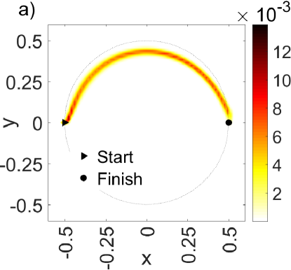
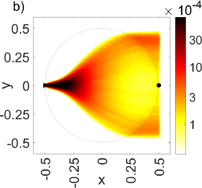
Figure 3: Heatmaps of the probability density $P(\bm{r},t)$ of the active particle for being at a location $(x,y)$ at time $t$: a) curved and b) straight optimal paths. The dashed line indicates the extension of the potential. Parameters are $U_{0}=0.22$, $D_{R}L/v_{0}=1$, and $\alpha=mB/k_{B}T=10$, where $k_{B}T=4\cdot 10^{-21}\text{kg m}^{2}/\text{s}^{2}$ is thermal energy at room temperature.

We have integrated the particle dynamics using Eq. (2) and the orientation unit vector $\bm{e}(t)=\bm{e}_{\text{opt}}(t)+\delta\bm{e}(t)$. Without thermal noise, $\bm{e}(t)=\bm{e}_{\text{opt}}(t)$, the active particle moves on the optimal trajectory. With thermal noise included a single active-particle trajectory will deviate from the optimal path. Figure 3 shows heat maps of the probability density $P(\bm{r},t)$ of the active particle for being at a location $(x,y)$ at time $t$ determined from 10000 simulated trajectories. The potential strength is $U_{0}=0.22$, where the straight trajectory is still the fastest one but also the curved trajectory gives a local minimum of the travel time. The aligning field strength is quantified by $mB=10k_{\text{B}}T$. While the trajectories curving around the potential barrier are close to the optimal path (a), the straight trajectory is strongly disturbed by the fluctuations in the orientation and the desired final position around $(x,y)=(0.5,0)$ is hardly reached (b). Thus, potential maxima drive active particles strongly away from optimal paths since the active particle cannot react appropriately on the fluctuating orientation.

Here, reinforcement learning comes in. In addition to being active the particle is also smart. It can sense its environment to determine its state, which in our implementation means the current location. Then the particle reacts by choosing a favorable orientation (action) in order to ultimately move on the optimal path.

4 Reinforcement Learning

Reinforcement learning is part of the developments in machine learning and artificial intelligence [57]. It provides a means how the smart active particle (agent) learns the optimal action for each state in order to achieve its specific goal of the fastest trajectory. To do so, the agent follows a policy, which is improved in repeated cycles of actions called episodes, and ultimately finds the optimal policy. In our case, an episode means moving from start to finish and the optimal policy guides the active particle on the shortest path.

We rely here on the method of $Q$ learning, one of the many variants of reinforcement learning [57]. The action-value function $Q(s,a)$ is a matrix, which depends on the possible states $s$ and the possible actions $a$. In our case they mean location of the smart particle on a grid and moving to one of the 4 neighboring grid points, respectively. Part of the policy is that for a given state $s$ the action $a$ with the largest value $Q$ is chosen, which brings the system into a new state $s^{\prime}$. Then, the action-value function for the specific state-action pair $(s,a)$ is updated according to [57]

$$Q(s,a)\leftarrow Q(s,a)+\alpha[R+\gamma\,\underset{a^{\prime}}{\mathrm{max}}\,Q(s^{\prime},a^{\prime})-Q(s,a)]\,.$$ (8)

Here, $R(s,a)$ is the reward associated with performing action $a$ on state $s$ and the second term in square brackets takes into account the future action value associated with the new state $s^{\prime}$ weigthed by the discount factor $\gamma$. Thus, $Q(s,a)$ increases when reward and future actions are favorable and $\alpha$ determines the learning speed. Starting with a constant action-value function [57], e.g., $Q(s,a)=100$ at the beginning of the first episode, $Q(s,a)$ changes during each episode, where one tries to steer the active particle. Thus, the next episode starts with an “improved” $Q$ function. It can be proven that $Q(s,a)$ becomes optimal after going through many episodes [61], meaning the active particle has ultimately learned to move on the optimal or shortest trajectory.

This deterministic procedure is often combined with the $\epsilon$-greedy method. In each state the action with the largest $Q$ value is only taken with probability $1-\epsilon$, so that also random actions are allowed. This guarantees a balance between exploiting the largest immediate reward but also exploring other actions, which might ultimately lead to a more optimal way of achieving the goal. Typically, $\epsilon$ is decreased with each episod, for example according to $\epsilon=1-i/i_{\text{max}}$, assuming that the $Q$ function has found its optimal value after $i_{\text{max}}$ episodes.

5 Optimization by smart active particle

We now apply the method of reinforcement learning to the optimization of the travel time of active particles in the Mexican hat potential of Eq. (5), which we treated in the beginning. We constrain the particles to move on a grid, which covers the plane in the region $[-0.75,0.75]\times[-0.75,0.75]$ and has a total of $43\times 43=1849$ grid points with a linear spacing $a=1.5/42=0.0357$ [see Fig. 4a) and b)]. The active particle can only move into four directions to the nearest neighbours (left, right, up, and down) as dictated by the action-value function $Q(s,a)$. We indicate the directions by unit vectors $\bm{d}_{i}$. When the particle reaches the border of the allowed region, the move out of the region is forbidden. The particle trajectory ends when the final position is reached.

Choosing the parameters in $Q(s,a)$ is not obvious and one performs a lot of testing. Crucial is the immediate reward for the current action. Since we want to minimize travel time, we set $R=-dt/1000$, where $dt=a/\bm{v}\cdot\bm{d}_{i}$ is the time to make the move to the neighboring grid point in the direction $\bm{d}_{i}$ under the influence of the potential force. When calculating the velocity, we always choose the active orientation $\bm{e}$ such that $\bm{v}=\bm{e}+\bm{F}\,\|\,\bm{d}_{i}$. Clearly, if the move is fast, $R$ is only mildly negative, whereas slow moves are unfavorable. Note, $dt<0$ corresponds to an unphysical move since it cannot be performed into the $\bm{d}_{i}$ direction. Thus, we choose a large negative reward $R=-10$ but still continue towards the end of the episod and set the travel time to infinity. Finally, reaching the end point is rewarded by $R=10$. Our studies with a constant greedy parameter $\epsilon=0.6$ show that the learning rate $\alpha$ speeds up the convergence of the $Q$ function in time, so we choose $\alpha=0.9$ (see supplemental material). In more complex potentials smaller values might be useful for not getting trapped in local mimima. Furthermore, in our problem a favorable discount factor is $\gamma=0.8$. Making it too small means that future rewards are not important, while choosing it close to one the immediate reward $R$ becomes less important (see supplemental material). Finally, for the linearly decreasing $\epsilon=1-i/i_{\text{max}}$ in the $\epsilon$-greedy method, $i_{\text{max}}=5000$ was chosen to be sure that the $Q$ function converged (see supplemental material).

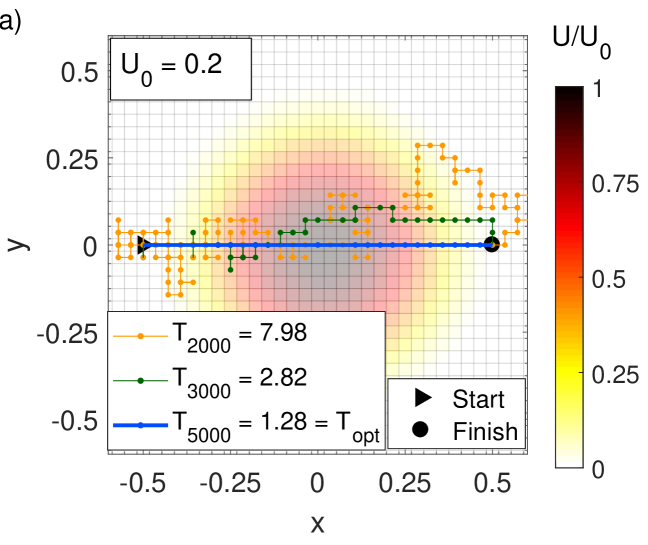
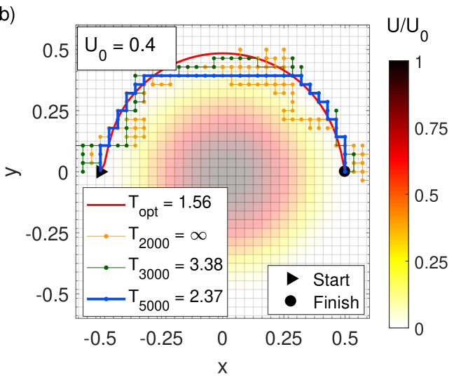
Figure 4: Trajectories of a smart active particle at the end of different episodes $i$ during $Q$ learning. The particle moves on a grid in the Mexican hat potential without brim (color-coded) from $x=-0.5$ to $x=0.5$: a) potential strength $U_{0}=0.2$ and b) $U_{0}=0.4$. $T_{i}$ is the travel time of the trajectory in episode $i$ and $T_{\text{opt}}$ the optimal travel time. The travel time $T_{2000}$ in b) is infinite since the particle performs unphysical steps. Note, the particle moves on the centers of the square unit cells.

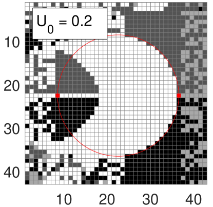
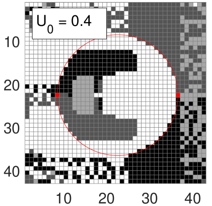
Figure 5: Represenation of the optimal action-value function $Q(s,a)$ at the end of the last episode for the smart active particle moving in the Mexican hat potential without brim. Left: for the straight trajectory ($U_{0}=0.2$) and Right: for the curved trajectory ($U_{0}=0.4$). For each position $s$ the action $a$ with the largest $Q$ is indicated. The matrix elements indexed by pairs from $[1,43]\times[1,43]$ correspond to grid points in the region $[-0.75,0.75]\times[-0.75,0.75]$ in the $x$-$y$ plane.

In Fig. 4 we now show two examples how the trajectories of the smart active particle evolves towards the optimal or shortest path with increasing number of episodes. The smart active particle “learns” to move on the optimal trajectory and stores its knowledge in the action-value function. In the beginning of the first episode the particle performs a random walk in the potential since with the initial value $Q(s,a)=100$ for all state-action pairs no experience is stored (see supplemental material). However, after going through more and more episodes the motion of the active particle becomes directed but still contains elements of a random walk. This is still visible in Fig. 4a) for the orange trajectory of epsiode $i=2000$. Ultimately, after $5000$ epsiodes the active particle has found the straight optimal path as expected for the potential height $U_{0}=0.2$ and the travel time coincides with the optimal value. For larger potential heights [$U_{0}=0.4$ in Fig. 4b)] we can also identify the curved trajectory as the optimal one. However, the optimal trajctory learned in the repeating epsiodes deviates from the exact solution since we only allow steps in the main directions of the grid. Adding also steps along the diagonal and making the step size smaller would improve the shape of the optimal trajectory resulting from $Q$ learning and also better approximate the optimal travel time. The final or optimal action-value function $Q(s,a)$ is represented in Fig. 5. It is the result of the learning process of the smart active particle for the optimization problem.

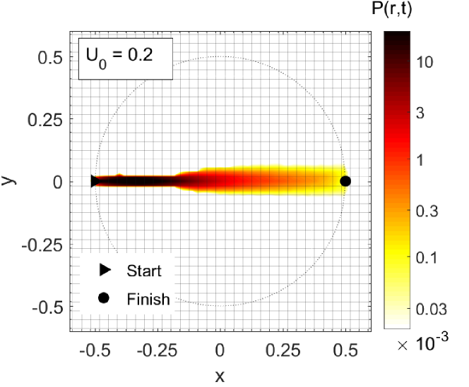
Figure 6: Heatmap of the probability density $P(\bm{r},t)$ of the active particle for being at a location $(x,y)$ at time $t$ for the straight optimal path determined by the optimal $Q$ function of Fig. 5 and under the influence of thermal noise. The dashed line indicates the extension of the potential. Parameters are $U_{0}=0.2$, $D_{R}L/v_{0}=1$, and $\alpha=mB/k_{B}T=10$, where $k_{B}T=4\cdot 10^{-21}\text{kg m}^{2}/\text{s}^{2}$ is thermal energy at room temperature.

We now address the influence of (thermal) noise on the learned optimal trajectories. In Fig. 3b) we saw that the straight path is unstable against fluctuations. How do the optimal trajectories behave under the learned strategy in combination with noise? To investigate this, we calculate the active orientation $\bm{e}_{\text{opt}}$ that belongs to the optimal directon $\bm{d}_{i}$ as determined by the optimal action-value function $Q(s,a)$. However, instead of proceeding with the step to the center of the neighboring square unit cell, we perform a Langevin dynamics simulation. We let $\bm{e}$ fluctuate around $\bm{e}_{\text{opt}}$ and integrate Eqs. (2) and (7) until the particle crosses the border to one of the neighboring unit cells. Then the process is repeated. While the heatmap for the learned curved trajectory looks similar to Fig. 3 a), the straight trajectory is stable under flucatuation as Fig. 6 shows since the $Q(s,a)$ function brings the smart active particle back on track when entering a neighboring unit cell. This clearly demonstrates the advantage of $Q(s,a)$, which tells the particle how to move even on locations outside the optimal path.

In this article we formulated and discussed the optimization problem for steering an active particle on the fastest path in a potential landscape and applied it to the Mexican hat potential without brim and one example of a more complicated potential. We demonstrated that an optimal path which crosses a potential barrier is very volatile to thermal noise added to the steered orientation. We then looked at a smart active particle and applied $Q$ learning as a special branch of reinforcement learning. We showed how in repeating episodes the smart particle learns to move on an optimal trajectory by storing its gained knowledge in the optimized action-value function. Now, thermal noise in the orientation does hardly affect the optimal path across a potential barrier since the optimized $Q$ function brings the smart active particle back on track.

We hope this article motivates further research on how reinforcement learning is applied to actively moving entities, in particular, to artificial or biological microswimmers in order to navigate optimally in a complex environment. A challenge is, of course, to develop ideas and principles to make a microswimmer smart meaning it can sense its environment and learn the optimal action. To mimic such a smart microswimmer, systems with an external information processing as in Refs. [47] and [48] are a first appealing step.

- [1] \NameRamaswamy S. \REVIEWAnnu. Rev. Condens. Matter Phys.12010323.
- [2] \NameMarchetti M., Joanny J., Ramaswamy S., Liverpool T., Prost J., Rao M. Simha R. A. \REVIEWRev. Mod. Phys.8520131143.
- [3] \NameElgeti J., Winkler R. G. Gompper G. \REVIEWRep. Prog. Phys.782015056601.
- [4] \NameCates M. E. Tailleur J. \REVIEWAnnu. Rev. Condens. Matter Phys.62015219.
- [5] \NameZöttl A. Stark H. \REVIEWJ. Phys.: Condens. Matter282016253001.
- [6] \NameBechinger C., Di Leonardo R., Löwen H., Reichhardt C., Volpe G. Volpe G. \REVIEWRev. Mod. Phys.882016045006.
- [7] \NameWaisbord N., Lefèvre C. T., Bocquet L., Ybert C. Cottin-Bizonne C. \REVIEWPhys. Rev. Fluids12016053203.
- [8] \NameMeng F., Matsunaga D. Golestanian R. \REVIEWPhys. Rev. Lett.1202018188101.
- [9] \NamePedley T. Kessler J. \REVIEWAnnu. Rev. Fluid Mech.241992313.
- [10] \NameDrescher K., Leptos K. C., Tuval I., Ishikawa T., Pedley T. J. Goldstein R. E. \REVIEWPhys. Rev. Lett.1022009168101.
- [11] \NameDurham W. M., Kessler J. O. Stocker R. \REVIEWScience32320091067.
- [12] \NamePalacci J., Cottin-Bizonne C., Ybert C. Bocquet L. \REVIEWPhys. Rev. Lett.1052010088304.
- [13] \NameEnculescu M. Stark H. \REVIEWPhys. Rev. Lett.1072011058301.
- [14] \NameWolff K., Hahn A. M. Stark H. \REVIEWEur. Phys. J. E36201343.
- [15] \NameTen Hagen B., Kümmel F., Wittkowski R., Takagi D., Löwen H. Bechinger C. \REVIEWNat. Commun.520144829.
- [16] \NameGinot F., Theurkauff I., Levis D., Ybert C., Bocquet L., Berthier L. Cottin-Bizonne C. \REVIEWPhys. Rev. X52015011004.
- [17] \NameKuhr J.-T., Blaschke J., Rühle F. Stark H. \REVIEWSoft Matter1320177548.
- [18] \NameSokolov A. Aranson I. S. \REVIEWPhys. Rev. Lett.1032009148101.
- [19] \NameRafaï S., Jibuti L. Peyla P. \REVIEWPhys. Rev. Lett.1042010098102.
- [20] \NameZöttl A. Stark H. \REVIEWPhys. Rev. Lett.1082012218104.
- [21] \NameUppaluri S., Heddergott N., Stellamanns E., Herminghaus S., Zöttl A., Stark H., Engstler M. Pfohl T. \REVIEWBiophys. J.10320121162.
- [22] \NameZöttl A. Stark H. \REVIEWEur. Phys. J. E3620134.
- [23] \NameLópez H. M., Gachelin J., Douarche C., Auradou H. Clément E. \REVIEWPhys. Rev. Lett.1152015028301.
- [24] \NameClement E., Lindner A., Douarche C. Auradou H. \REVIEWEur. Phys. J. Spec. Top.22520162389.
- [25] \NameSecchi E., Rusconi R., Buzzaccaro S., Salek M. M., Smriga S., Piazza R. Stocker R. \REVIEWJ. R. Soc. Interface13201620160175.
- [26] \NameTheurkauff I., Cottin-Bizonne C., Palacci J., Ybert C. Bocquet L. \REVIEWPhys. Rev. Lett.1082012268303.
- [27] \NamePohl O. Stark H. \REVIEWPhys. Rev. Lett.1122014238303.
- [28] \NameSaha S., Golestanian R. Ramaswamy S. \REVIEWPhys. Rev. E892014062316.
- [29] \NameLiebchen B., Marenduzzo D., Pagonabarraga I. Cates M. E. \REVIEWPhys. Rev. Lett.1152015258301.
- [30] \NameSimmchen J., Katuri J., Uspal W. E., Popescu M. N., Tasinkevych M. Sánchez S. \REVIEWNat. Commun.7201610598.
- [31] \NameStark H. \REVIEWAcc. Chem. Res5120182681.
- [32] \NameStürmer J., Seyrich M. Stark H. \REVIEWJ. Chem. Phys.1502019214901.
- [33] \NameAgudo-Canalejo J. Golestanian R. \REVIEWPhys. Rev. Lett.1232019018101.
- [34] \NameRühle F., Blaschke J., Kuhr J.-T. Stark H. \REVIEWNew J. Phys.202018025003.
- [35] \NameThutupalli S., Geyer D., Singh R., Adhikari R. Stone H. A. \REVIEWPNAS11520185403.
- [36] \NameShen Z., Würger A. Lintuvuori J. S. \REVIEWSoft Matter1520191508.
- [37] \NameChepizhko O., Altmann E. G. Peruani F. \REVIEWPhys. Rev. Lett.11020131.
- [38] \NameChepizhko O. Peruani F. \REVIEWPhys. Rev. Lett.11120131.
- [39] \NameReichhardt C. Olson Reichhardt C. J. \REVIEWPhys. Rev. E902014012701.
- [40] \NameZeitz M., Wolff K. Stark H. \REVIEWEur. Phys. J. E40201723.
- [41] \NameLeonardo R. D., Angelani L., Dell‘Arciprete D., Ruocco G., Lebba V., Schippa S., Conte M. P., Mecarini F., Angelis F. D. Fabrizio E. D. \REVIEWPNAS10720109541.
- [42] \NameSokolov A., Apodaca M. M., Grzybowski B. A. Aranson I. S. \REVIEWPNAS1072010969.
- [43] \NamePototsky A., Hahn A. M. Stark H. \REVIEWPhys. Rev. E872013042124.
- [44] \NameKaiser A., Peshkov A., Sokolov A., ten Hagen B., Löwen H. Aranson I. S. \REVIEWPhys. Rev. Lett.1122014158101.
- [45] \NameReichhardt C. J. O. Reichhardt C. \REVIEWAnnu. Rev. Condens. Matter Phys.8201751.
- [46] \NameMano T., Delfauc J.-B., Iwasawaa J. Sano M. \REVIEWPNAS1142017E2580.
- [47] \NameBäuerle T., Fischer A., Speck T. Bechinger C. \REVIEWNature Com.920183232.
- [48] \NameKhadka U., Holubec V., Yang H. Cichos F. \REVIEWNature Com.920183864.
- [49] \NameSchmidt F., Liebchen B., Löwen H. Volpe G. \REVIEWJ. Chem. Phys.1502019094905.
- [50] \NameVolpe G. Volpe G. \REVIEWPNAS114201711350.
- [51] \NameNava L. G., Großmann R. Peruani F. \REVIEWPhys. Rev. E972018042604.
- [52] \NameLiebchen B. Löwen H. \REVIEWarXiv:1901.08382v12019.
- [53] \NameTröltzsch F. \BookOptimal Control of Partial Differential Equations: Theory, Methods, and Applications Graduate Studies in Mathematics (American Mathematical Society) 2010.
- [54] \NameSritharan S. S. \BookOptimal Control of Viscous Flow Miscellaneous Titles in Applied Mathematics Series (Society for Industrial and Applied Mathematics) 1998.
- [55] \NameProhm C., Tröltzsch F. Stark H. \REVIEWEur. Phys. J. E3620131.
- [56] \NameSoner M. \BookStochastic Optimal Control in Finance Cattedra Galileiana (Edizioni della Normale) 2005.
- [57] \NameSutton R. S. Barto A. G. \BookReinforcement Learning: An Introduction 2nd Edition (MIT Press, Cambridge) 2018.
- [58] \NameReddy G., Celani A., Sejnowski T. J. Vergassola M. \REVIEWPNAS1132016E4877.
- [59] \NameColabrese S., Gustavsson K., Celani A. Biferale L. \REVIEWPhys. Rev. Lett.1182017158004.
- [60] \NameMuiños-Landin S., Ghazi-Zahedi K. Cichos F. \REVIEWarXiv:1803.06425v22018.
- [61] \NameJaakkola T., Jordan M. I. Singh S. P. \REVIEWNeural Comput.619941185.