Scene Recognition with Prototype-agnostic Scene Layout

Abstract

Exploiting the spatial structure in scene images is a key research direction for scene recognition. Due to the large intra-class structural diversity, building and modeling flexible structural layout to adapt various image characteristics is a challenge. Existing structural modeling methods in scene recognition either focus on predefined grids or rely on learned prototypes, which all have limited representative ability. In this paper, we propose Prototype-agnostic Scene Layout (PaSL) construction method to build the spatial structure for each image without conforming to any prototype. Our PaSL can flexibly capture the diverse spatial characteristic of scene images and have considerable generalization capability. Given a PaSL, we build Layout Graph Network (LGN) where regions in PaSL are defined as nodes and two kinds of independent relations between regions are encoded as edges. The LGN aims to incorporate two topological structures (formed in spatial and semantic similarity dimensions) into image representations through graph convolution. Extensive experiments show that our approach achieves state-of-the-art results on widely recognized MIT67 and SUN397 datasets without multi-model or multi-scale fusion. Moreover, we also conduct the experiments on one of the largest scale datasets, Places365. The results demonstrate the proposed method can be well generalized and obtains competitive performance.

I Introduction

Scene images (e.g., “classroom”, “bedroom”) are usually composed of specific semantic regions (e.g., “desk”, “bed”) distributed in certain spatial structures. Exploring the local regions and their spatial structures has been a long-standing research direction and plays a crucial role in scene recognition [1, 2, 3]. Due to the size and location changes of semantic regions (see Fig. 1), the spatial structures of images have great diversity, which makes it very difficult to represent them so as to adapt various image characteristics. Thus, how to build and model such structural layout into image representations is an obstacle problem.

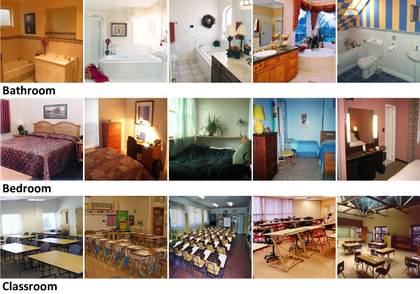
Figure 1: Image examples from MIT67 datasets. Here shows the images from three scene categories (“bathroom”, “bedroom”, and “classroom”). It can be seen that the objects in each scene can vary greatly in size and location, like “bathtub” in scene “bathroom”, “bed” in scene “bedroom”, “desk” in scene “classroom”.

Most existing methods [4, 3, 5, 6] model spatial structural information based on predefined grid regions or densely sampled regions. These regions are in fixed sizes located in a grid, forming a simple and constant structure as a common prototype for all images, which results in rigid layout even with the extension of multi-scale setting. Some earlier works [1, 7, 2] have attempted to learn several prototypes for each category images with different models, such as constellation model in [1], Deformable Part-based Model (DPM) in [7] and DPM’s variant in [2]. These prototypes can be regarded as templates with fixed topological structures for each scene category, where the geometric relations of the components are obtained through statistic learning. The spatial structure of each image is constructed by conforming to the prototypes. Although more than one prototype is usually used to characterize one scene category, such limited variety is not comprehensive enough to cover the large intra-class structural diversity of scene images. In contrast, our motivation is to design a layout modeling framework to flexibly capture the unconstrained spatial structures and effectively obtain discriminative patterns from them.

In this paper, we propose Prototype-agnostic Scene Layout (PaSL) construction method, which builds spatial structure for each single image without conforming to any prototype. Given an image, PaSL is constructed with the locations and sizes of discriminative semantic regions, which are detected by only using the convolutional activation maps of this image. Thus, PaSLs will vary from image to image and can flexibly express different spatial characteristics of the images. Considering the natural property of the graph to preserve diverse and free topological structures, we frame the structural modeling process as a graph representation learning problem. More specifically, we propose Layout Graph Network (LGN) where regions in PaSL are defined as nodes and two kinds of relations between nodes are encoded as edges. Through the graph convolution [8] and mapping operations of LGN, the topological structure and region representations can be transformed into a discriminative image representation.

The main idea of PaSL construction method is inspired by the ability of pretrained CNNs to localize the meaningful semantic parts [9]. We make use of the convolution activation maps extracted from pretrained CNNs to detect semantic regions, and aggregate them to generate discriminative regions and form PaSL in an unsupervised way. The advantages of our method is two folds. One is that the whole process is performed on each image independently and can be easily extended to large scale datasets. Another is that PaSLs derived from different pretrained CNNs can yield comparable performances with same LGN, which demonstrates they have considerable generalization ability. Besides constructing PaSL, modeling it in graph structure is also an important contribution in this paper. Conventional structural models in scene recognition either have difficulty of optimization [7, 2] on large scale datasets or simplify the structural information [3, 10]. In contrast, we build Layout Graph Network upon PaSL by reorganizing it as a layout graph containing two subgraphs. These two subgraphs aim to capture different kinds of relations, spatial and semantic similarity relations between regions, respectively. Thanks to the independence between these two kinds of relations, we can explore structural information in a higher order space and easily encode it into more discriminative features. Furthermore, the application of graph convolution makes our model effectively handle various topological structures and easy to be optimized with large amounts of data.

We evaluate our model on three widely recognized scene datasets, MIT67 [1], SUN397 [11], and Places365 [12]. The ablation study shows that our method obtains up to $5\%$ improvements over baselines that neglect structural information. Compared to current works on MIT67 and SUN397 that benefit from multi-model or multi-scale fusion methods, our model even outperforms them and obtains state-of-the-art results with single model in single scale. When extending our model to one of the largest scale dataset, Places365, it still shows competitive performance.

II Related Work

II-A Scene Recognition

In early works, bag-of-feature methods (like VLAD [13], Fisher Vector [14]) with handcrafted features (like SIFT [15]) have demonstrated great power on scene recognition. However, these methods incorporate local information in an orderless way, which loses spatial dependencies between local regions. Then, some works further explore the spatial contextual dependencies within bag-of-feature methods. Lazebnik et al. [16] proposed Spatial Pyramid Matching to exploit approximate spatial information in a predefined grid. Parizi et al. [17] used a reconfigurable model operated on a grid to capture the spatial information among regions.

Beyond this simple and fixed spatial information based on grids, some works explore the complex and flexible spatial structures formed by scene components in different ways. These works [1, 7, 2] construct the scene structures in a similar way to Deformable Parts Model (DPM) [7], DPM’s variant [2], or a constellation model [1]. Based on these structural models, a fixed number of structures for each scene category, which can be named as scene prototypes, are learned. Then the spatial structural information of each image is discovered by conforming to the default structure of the most matched scene prototype. The spatial structures derived from scene prototypes have difficulty covering the intra-class variety of scenes. Differently, our approach can model the structural layout for each image following its own characteristics.

Recently, Deep Learning methods, especially Convolution Neural Networks, have been widely used in scene recognition. Some works [18, 19, 6, 20] combine bag-of-feature methods (like VLAD, Fisher Vector) or dictionary-based method with CNN to explore discriminative local information in an orderless way. To model spatial contextual dependencies, the works [3, 10] learn a sequential model (like LSTM [3]) or a graphical model (MRF [10]) on fixed size regions. Furthermore, the multi-scale strategy is adopted to capture more precise local information. However, these works either encounter the problem of noise regions caused by predefined grids, or simplify the spatial structural information, while our method can explore the complex spatial structural layouts and reform them in graphs to generate discriminative representations.

II-B Discriminative Region Discovery

To discover the discriminative regions has been a long-standing study in visual recognition. Singh et al. [21] use an iterative optimization procedure to alternately clustering and training discriminative classifier on densely sampled patches. Juneja et al. [22] first propose an initial set of regions based on low-level segmentation cues, and then learn detectors on top of these regions. However, these works all use the handcrafted features as region representations.

Recently, Some works take advantage of CNN activations as region descriptors for discriminative region discovery. Wu et al. [4] obtain region proposals by performing MCG, and screen the regions by using one-class SVM and RIM clustering. Cheng et al. [23] sample a set of local patches in a uniform grid with their object scores extracted from ImageNet-CNN, then discard the patches containing non-discriminative objects by applying Bayes rules. One common characteristic of these works is that they generate the candidate regions independently of the CNN classifiers, which will incur much additional computational cost.

Besides these aforementioned approaches, some recent works explore the convolutional responses from CNNs to directly discover discriminative regions for fine-grained object recognition. Zheng et al. [24] group the convolutional channels to localize object parts in the well constrained spatial configurations. Wei et al. [25] use a simple thresholding method to discover object parts and select the largest component to represent the desired foreground object. In contrast, we formulate the discovery procedure for scene recognition, where more complex semantic regions and unconstrained spatial structures exist. Similarly, the work of [5] also uses a pretrained CNN classifier to generate discriminative regions for scene images. However, it needs extra scene category cue for each image and the CNNs with a specific architecture.

II-C Graph Neural Networks in Computer Vision

Graph Neural Networks (GNNs) are designed to deal with the graph structured data, which were first proposed in [26]. Recently, some variants have been applied in program verification [27], molecular property prediction [28], document classification [8] and made significant progress. Inspired by the success of GNNs on graph structured data, some researches apply them in computer vision task, like multi-label classification [29], situation recognition [30], scene graph generation [31], zero-shot recognition [32], and etc. These works apply GNNs to natural graph data (like knowledge graph [29, 30, 32]), or constructed graph data with the supervision of annotated object regions (like scene graph [31]). In contrast to them, we perform GCN [8], a variant of GNN, on the structural layouts in scene images without external knowledge or object annotations.

III Our Approach

In this section, we first introduce how to construct Prototype-agnostic Scene Layout (PaSL) from pretrained CNNs in an unsupervised way. Then we build Layout Graph Network upon PaSL to integrate structural information into visual representations. In the following, we will go into details about our approach.

III-A Prototype-agnostic Scene Layout Construction

PaSL is constructed by the locations and sizes of discriminative regions (including objects, object-parts, and other visual patterns) in each image. To form PaSL, we first need to discover discriminative regions. Unlike previous works that use many selected image patches (from manual annotation [2] or region proposal [4]) to train region detectors, we only need the convolutional units from a pretrained CNN, without detector training.

Recently, Zhou et al. [33] have shown the convolutional units from a CNN pretrained on Places [34] dataset can be used as object detectors. And Bau et al. [9] extend this conclusion to more pretrained CNNs and more visual concepts. They demonstrated the individual convolutional units in CNN can be aligned with semantic concepts across a range of objects, parts, textures, scenes, materials, and colors. Inspired by these works, we utilize the convolutional units in pretrained CNNs as region detectors. In practice, given an image, we feed it into a pretrained CNN to extract the convolutional activation maps $\mathcal{A}$ ($\mathcal{A}\in R^{H\times W\times C}$) from the last convolutional layer (For VGG16, max pooling need to be employed). The $c$-th activation map in $\mathcal{A}$ is represented as $\mathcal{A}_{c}\in\mathbb{R}^{H\times W}$, while $c\in\{1,\cdots,C\}$. For instance, if the resolution of the input image is $224\times 224$, we obtain $7\times 7\times 512$ activation maps as $\mathcal{A}$, where $H=W=7$ and $C=512$, by adopting a pretrained VGG16 model.

Based on the same assumption of [33, 9] that the desired regions (e.g., semantic regions) in feature maps have high response values, we propose an adaptive threshold $T$ in Eq.1 to detect the candidates of discriminative regions.

$$T=\frac{1}{C}\sum_{c=1}^{C}\dot{\mathcal{A}}_{c},\ \ \dot{\mathcal{A}}_{c} =\max\left(\mathcal{A}_{c}\right)$$ (1)

For efficient computing, any activation map whose maximum value is under $T$ is discarded, then a subset $\widetilde{A}$ of activation maps $\mathcal{A}$ is produced. Each activation map in $\widetilde{A}$ is scaled up to the input image resolution and then thresholded into a binary map $B$ by using the threshold $T$. We take the connected components in $B$ as the candidates of discriminative regions. The algorithm from [35] is adopted to generate bounding boxes of the connected components in each binary map. By performing the same operations on all activation maps in $\widetilde{A}$, we obtain bounding box set $M$ of all candidates of discriminative regions. The element $m$ in $M$ is composed of the left-up and right-bottom coordinates, e.g., $m=\{x_{min},\thinspace y_{min},\thinspace x_{max},\thinspace y_{max}\}$, where $(x_{min},\thinspace y_{min})$ denotes the coordinate of left-up point in bounding box, and $(x_{max},\thinspace y_{max})$ is the coordinate of right-bottom point.

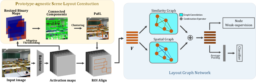
Figure 2: Overview of our approach. A pretrained CNN model (like VGG16 or ResNet50) is used as the backbone to extract the candidates of discriminative regions. The desired discriminative regions are clustered from these candidates, and fed into ROI Align Layer to generate the node representations. Two subgraphs are constructed by treating regions as nodes and designing spatial or similarity relation as edge. Then, we perform graph convolution on two subgraphs and combine them to obtain the final node representations. Finally, node weak-supervision mechanism makes each node predict global image category by feeding it into a fully-connected layer. Meanwhile, the averagely pooled node representations, regarded as the global image representations, are exploited for scene recognition by a fully-connected layer.

In practice, the number of elements in $M$ is large, e.g., $\sim 500$ for VGG16 and $\sim 1500$ for ResNet50. If we construct PaSL with all regions from $M$, it will cause expensive computational cost in the later process. Meanwhile, the regions from $M$ have two characteristics. One is that although adaptive thresholding can discard some small noise parts, there also have several wrong detected results imposed by the unsupervised process. Another one is that discovering from each activation map independently may bring many visually similar regions. In order to avoid the wrong or similar regions, we choose a simple yet effective way, e.g., clustering, to find the most representative regions in $M$ as the desired discriminative regions. Accordingly, the discriminative regions $D$ could be obtained by:

$$L =\mathbb{C}(M,\thinspace N)$$ (2)

$$D =\mathit{Aggre}(M,\thinspace L)$$ (3)

where $\mathbb{C}(\cdot)$ denotes hierarchical clustering method. $N$ stands for the number of clusters, which also means the number of discriminative regions. $L$ corresponds to the cluster labels of the elements in $M$. Given cluster labels $L$, we perform mean pooling method ($\mathit{Aggre}$) on bounding boxes of elements in the same cluster to obtain bounding boxes of discriminative regions $D=\{d_{1},\thinspace\dots,\thinspace d_{N}\}$. Specifically, clustering method can be k-means or spectral clustering. If choosing k-means, cluster centers can be directly used as discriminative regions.

Given discriminative regions, we define Prototype-agnostic Scene Layout (PaSL) as a collection of the locations and sizes of these regions in each image. The whole process is shown in Fig. 2. The spatial structure, that is implicit in PaSL, requires to be represented in a certain form. To form the diverse and free topological structure of PaSL of each image, the graph is adopted as data structure. Following the common setting of graph structured data, we define the discriminative regions as nodes and encode two kinds of independent relations between regions as edges. The details will be described in the following section.

III-B Layout Graph Network

For modeling the spatial structure of PaSL, we reorganize it as a layout graph, which is better for incorporating the structural information into visual representations. Given PaSL with discriminative regions, a layout graph $\mathcal{G}=\{\mathit{V},\thinspace\mathbf{\mathit{A^{sp}}},\thinspace\mathit{A^{sim}}\}$ is constructed, which contains a node set $\mathit{V}$, and two adjacency matrices $\mathit{A^{sp}}$, $\mathit{A^{sim}}$. For clarity, we decompose the layout graph into two subgraphs with the same nodes but different adjacency matrices: spatial subgraph $\mathcal{G}^{sp}=\{\mathit{V},\thinspace\mathit{A}^{sp}\}$ and similarity subgraph $\mathcal{G}^{sim}=\{\mathit{V},\thinspace\mathit{A}^{sim}\}$. More specifically, these two subgraphs share the same node set $V=\{v_{1},\thinspace\dots,\thinspace v_{N}\}$, where $v_{i}$ corresponds to the representation of discriminative region $i$. We apply RoIAlign [36] to extract the representation of each region from a pretrained CNN as the initial state vector of $v_{i}$. This pretrained CNN can be regarded as a feature extraction model, which is same as the pretrained model for generating PaSL, unless otherwise stated.

Spatial Subgraph. The spatial information is vital in PaSL, because it implies the functions or properties of regions. One way to take advantage of this information is to exploit the spatial relations between regions. Specifically, we define a kind of spatial representation to encode this relation and then generate the spatial edge to form the adjacency matrix. As mentioned above, each discriminative region $i$ has a bounding box $d_{i}=\{x_{min},\thinspace y_{min},\thinspace x_{max},\thinspace y_{max}\}$. Inspired by [37], we extract the spatial feature of each region as follows:

$$d_{i}^{sp}=\left[\frac{x_{min}}{W_{img}},\thinspace\frac{y_{min}}{H_{img}},\thinspace\frac{x_{max}}{W_{img}},\thinspace\frac{y_{max}}{H_{img}},\thinspace\frac{Ar}{Ar_{img}}\right]$$ (4)

where $Ar$ and $Ar_{img}$ are the areas of the region $i$ and the image respectively. $W_{img}$ and $H_{img}$ denotes the width and height of the image. We concatenate $d_{i}^{sp}$ and $d_{j}^{sp}$ to obtain the spatial representation $d_{ij}^{sp}$ of spatial relation between the regions $i$ and $j$. After generating the spatial representation, we employ an edge function $F_{e}$, implemented as one-layer fully connected network, to generate the spatial edge $a_{ij}^{sp}$ as:

$$e_{ij}^{sp} =F_{e}(d_{ij}^{sp})$$ (5)

$$a_{ij}^{sp} =\frac{\exp(e_{ij}^{sp})}{\sum_{j\neq i}\exp(e_{ij}^{sp})}$$ (6)

Then the spatial adjacency matrix $A^{sp}$ is obtained to form spatial subgraph $\mathcal{G}^{sp}$. The diagonal values in $A^{sp}$ are zero.

Similarity Subgraph. To explore the spatial information in PaSL is an obvious requirement. But there exists an problem in the spatial subgraph that the spatial relation overlooks the semantic meanings of regions. To address this problem, we propose the similarity subgraph as a complement to the spatial subgraph. Due to the lack of explicit labels for the local regions, we take the region representation as a substitution for the semantic label. Then, we model the similarity between these region representations to capture the semantic similarity relations between regions.

Given the node set $V$, we can obtain the state vector $v_{i}\in\mathbb{R}^{h}$ of each node. In similarity subgraph, we aim to obtain the strong connection between semantic similar regions. So the semantic similarity relations between regions are measured by the cosine similarity, which is defined as follows:

$$e_{ij}^{sim}=\phi(v_{i})^{T}\phi(v_{j}),\ \ \phi(v)=\frac{\omega^{sim}v}{\left|\left|\omega^{sim}v\right|\right|_{2}}$$ (7)

where $\phi$ represents the transformation of the state vector and following $\ell_{2}$ normalization, $\omega^{sim}\in\mathbb{R}^{h/2\times h}$ is the transformation weights. The dot product $e_{ij}^{sim}$ of two $\ell_{2}$ normalized vector denotes the cosine similarity between regions. To balance the impact of neighbor nodes, we perform the softmax function on each row of the cosine similarity matrix as:

$$a_{ij}^{sim}=\frac{\exp(e_{ij}^{sim})}{\sum_{j\neq i}\exp(e_{ij}^{sim})}$$ (8)

where $A^{sim}$ is used as the adjacency matrix for similarity subgraph. The diagonal values in $A^{sim}$ are zero.

Graph Convolution. After building the layout graph, the next step is to incorporate the spatial and semantic similarity information into the representations of regions, and generate discriminative image representations. Considering the superior performance of Graph Convolution Network (GCN) [8] on graph structured data, we adopt Graph Convolution (GC) on spatial and similarity subgraph, then combine two subgraphs. Given a graph $\mathcal{G}=\{V,\thinspace A\}$, where $V\in\mathbb{R}^{N\times h}$ is the node set and $A\in\mathbb{R}^{N\times N}$ is the adjacency matrix. One GC layer aims to combine the information of neighbor nodes and target node through relation edges to update the state vector of target node, which can be formulated as:

$$V^{t} =\sigma(ZV^{t-1}\Omega_{t})$$ (9)

$$Z=\Lambda^{-1}\tilde{A}$$

$$\Lambda_{ii}=\sum_{j}\tilde{A}_{ij},\ \ \tilde{A}=A+I_{N}$$

where $V^{t}$ is the updated state vectors of nodes in GC layer $t$, $\Omega_{t}\in\mathbb{R}^{h_{t-1}\times h_{t}}$ denotes weight matrix, and $h_{0}$ is the input vector dimension while $h_{t}\thinspace(t>0)$ means hidden size of GC layer $t$. We utilize the non-linear function ReLU as $\sigma$.

Combination of Different Subgraphs. Now, we can employ graph convolution to generate the updated state vectors $V_{sim}^{t}$, $V_{sp}^{t}$ for spatial, similarity subgraphs, with $A^{sim}$, $A^{sp}$ obtained above, respectively. Then, we investigate how to effectively combine these two subgraphs. First, we define the combination of two subgraphs as:

$$V^{t}=V_{sim}^{t}\oplus V_{sp}^{t}$$ (10)

where $\oplus$ means the combination operator. Intuitively, we can combine the updated state vectors from two subgraphs by using element-wise addition or maximum. Beyond them, we also consider an alternative to improve the sparsity of combined representations, which is element-wise product. we conduct a comparison experiment in section IV-D2, which confirms that the element-wise product is a better choice to combine two subgraphs.

Global information. PaSLs in most images cannot cover the whole areas of images, which may lose some useful information. So we decide to add global information into the layout graph. We define a global node that represents the whole image, and perform average pooling on the convolutional activation maps from the last convolutional layer to generate the initial state vector of the global node. As a result, the node set $V$ will be $\{v_{0},v_{1},\cdots,v_{N}\}$, where $v_{0}$ denotes the global node. For spatial subgraph, We set the bounding box of global node as $d_{0}=\{x_{min}=0,\thinspace y_{min}=0,\thinspace x_{max}=W_{img},\thinspace y_{max}=H_{img}\}$, where $W_{img}$ and $H_{img}$ denote the width and height of the whole image. The global node is connected to all local nodes, and we apply the same operations described above to obtain the new adjacency matrices $A^{sp}$, $A^{sim}$.

Output. To avoid overfitting, we only utilize one GC layer. We obtain the final state vectors $V^{1}\in\mathbb{R}^{N\times h_{1}}$ from the GC layer and following $\ell_{2}$ normalization as node representations. When only using local regions as nodes, we apply average pooling on node representations to generate the image representation as a $h_{1}$-dimensions vector. And if adding global node, we only treat the global node representation as the image representation. Besides, we have tried to averagely pool all global/local node representations to obtain the image representation, which hurts the performance. And we have also tried to concatenate the global node representation with averagely pooled local node representation to produce the image representation, while it has similar performance but needs more parameters in the later process. For scene recognition, we feed image representation into one layer fully connected network to predict the image category. And we utilize softmax function with cross entropy as the loss function to obtain the image classification loss $l_{g}$.

Node Weak-supervision Mechanism. Specifically, we propose a node weak-supervision mechanism to improve the discriminative performance of each node (except global node). For the representation of each node, we force it to predict the scene category of image by using one layer fully-connected network in a weakly supervised way, which can make the node representations more suitable for image recognition and produce the node classification loss $l_{n}$. We combine the two classification loss to form the total loss $l$ as,

$$l=l_{g}+\lambda l_{n}$$ (11)

where $\lambda$ is a hyperparameter. Specifically, this branch is only used in the training process.

IV Experiments and Discussions

In this section, we evaluate our method on three widely recognized datasets, MIT67 [1], SUN397 [11], and Places365 [12].

MIT67 Dataset contains a total of 15620 images belonging to 67 indoor scene categories. Following the standard evaluation protocol, we use 80 images of each category for training and 20 images for testing. We report accuracy as evaluation metric.

SUN397 Dataset is a more challenge scene dataset, which contains 397 scene categories and 108,754 images. The dataset is divided into 10 train/test splits, each split consists of 50 training images and 50 test images per category. The average accuracy over splits is presented as evaluation metric.

Places365 Dataset is one of the largest scale scene-centric datasets, which has two training subsets, Places365-standard and Places365-challenge. In this paper, we only choose Places365-standard as training set, which consists of around 1.8 million training images and 365 scene categories. The validation set of Places365 contains 100 images per category and the testing set has 900 images per category. We report experimental results on its validation set, because its test set has no available ground truth. Both top1 and top5 accuracy are reported as evaluation metric.

IV-A Implementation Details

Our model can be implemented with different pretrained models as backbone CNNs. For fair comparison with other methods, we adopt three pretrained models, which are VGG-IN, VGG-PL205, ResNet-PL365. VGG-IN, VGG-PL205 are the VGG16 models pretrained on ImageNet dataset [38] and Places205 dataset [34] respectively, ResNet-P365 is the ResNet50 model pretrained on Places365 dataset [12]. To construct PaSL, we extract the convolutional activation maps from the last convolutional layer (max-pooled in VGG16). Inspired by [39], we fix the input image resolution as $448\times 448$ for VGG16-IN and ResNet50-PL365, $352\times 352$ for VGG16-PL205, which leads to $14\times 14\times 512$, $14\times 14\times 2048$ and $11\times 11\times 512$ activation maps respectively. The number of clusters $N$, the hidden size $h_{1}$ and the $\lambda$ are set to $\{32,8192,4.0\}$ for LGN with backbone VGG-IN and VGG-PL205, $\{64,\thinspace 8192,\thinspace 1.0\}$ for ResNet-PL365.

The initial state vectors of nodes are normalized with two normalization function (Layer Normalization [40], $\ell_{2}$ Normalization), then fed into LGN. Specifically, the Layer Normalization is not trained in our experiments. We train LGN using Adam [41] with an initial learning rate of $10^{-3}$ (decayed by a factor of 0.1 at 10/15/18th epoch), a batch size of 32 and weight decay of $10^{-5}$. All parameters are randomly initialized following Xavier initialization method [42]. We use the model trained at 20th epoch as the final model in all experiments. Dropout is only applied on the output prediction layer with a ratio of $0.2$. The $\ell_{2}$-norm of gradients is clipped to a maximum value of $0.25$. All experiments are conducted on a single NVIDIA 1080 Ti GPU by using open-sourced framework Tensorflow.

IV-B Experimental Results

In this subsection, we first report the performances on MIT67, SUN397. These two datasets are the most popular benchmark for evaluating scene recognition methods. Thus, we can provide the comprehensive and detailed comparison with existing works about scene recognition. Meanwhile, we also conduct experiments on one of the largest scale scene dataset, Places365, to demonstrate the generalization of our model.

IV-B1 Comparison on single model in single scale (MIT67 and SUN397)

Most existing scene recognition methods obtain their best performances based on multi-model or multi-scale fusion. However, to perform the fusion needs more computational time and memory usage, which will cause expensive cost. The idea of multi-scale representation is presented to alleviate the problem of the various sizes of the semantic components in scene images. Benefiting from the flexible structure of PaSL, our model can efficiently capture the different locations and sizes of semantic components, to produce the better image representations for scene recognition. To prove it, we compare the previous works with our model on single VGG16 model in single scale in Table I. The two pretrained VGG16 models, pretrained on ImageNet (VGG-IN) and Places205 (VGG-PL205) are adopted as backbone CNN models in the comparison. The backbone VGG-PL205 show impressive performance on MIT67 and SUN397, generally outperforming the VGG-IN. Compared to existing works using the same VGG-PL205 backbone, our model obtains better performance with a clear margin ($1-2\%$). While based on the VGG-IN, the LGN surpasses the most previous works, except MFAFVNet and LSO-VLADNet. The lower performance of VGG-IN can be concluded into two possible reasons: 1) these two previous works report better accuracy benefiting from the refinement of low level convolutional features. 2) The PaSL derived from VGG-IN has less power for capturing the spatial structure in scene images, which is verified in subsection IV-C3.

TABLE I: Comparison of LGN with previous methods based on single VGG16 model in single scale. Classification accuracy (%) is reported as evaluation metric on MIT67 and SUN397 datasets. The best result of each column is marked in bold.

Method	P.S.	I.R.	MIT67	SUN397
VGG16 [39]	IN	643	76.42	59.71
MFA-FS [43]	IN	512	79.57	61.71
HSCFVC [44]	IN	512	79.5	-
MFAFVNet [19]	IN	512	80.3	62.51
CNN-DL [6]	IN	-	78.33	60.23
LSO-VLADNet [20]	IN	448	81.7	61.6
VGG16 [39]	PL205	256	80.90	66.23
S-HunA [45]	PL205	-	83.7	-
SpecNet [46]	PL205	256	84.3	67.6
CNN-DL [6]	PL205	-	82.86	67.90
LGN	IN	448	79.78	62.03
	PL205	352	85.37	69.48
P.S. : “Pretrain dataset”, I.S. : “Input Resolution”
IN : “ImageNet”, PL205 : “Places205”

IV-B2 Comparison with the state-of-the-art works (MIT67 and SUN397)

Table II presents the results of our best model and state-of-the-art works. Our best model is based on ResNet-PL365 pretrained model in single scale setting. Compared to the methods [5, 47, 48] based on the same pretrained model, our model achieves the best performance. Most importantly, the work [5] utilizes the similar technique to extract discriminative regions and even multi-scale regions to generate the image representations. However, it ignores the relations (either spatial or similarity relations) between local regions, leading to an inferior performance. This confirms that the relations between local regions are useful for scene recognition, and our LGN can take advantage of them. We also report state-of-the-art works that involve various combination techniques to achieve better performance. Even though these works contain multi-scale information [49, 43, 19, 6, 23, 5, 50] or multi-model combination [43, 19, 23, 48], our model still outperforms them and achieves the state-of-the-art performance for scene recognition, to the best of our knowledge.

TABLE II: Comparison of LGN with state-of-the-art works on MIT67 and SUN397. Classification accuracy (%) is reported as evaluation metric. The best result of each column is marked in bold.

Method	MIT67	SUN397
CLDL [49]	84.69	70.40
MFA-FS [43]	87.23	71.06
MFAFVNet [19]	87.97	72.01
CNN-DL [6]	86.43	70.13
SDO [23]	86.76	73.41
PowerNorm [47]	86.3	-
fgFV [50]	87.60	-
MFAFSNet [48]	88.06	73.35
Adi-Red [5]	-	73.59
LGN (ResNet)	88.06	74.06

IV-B3 Experimental results on Places365

To make more convincing results, we report the result of our best model on Places365 in Table III. The experimental setting is same as above, except the input resolution changes to $224\times 224$ and the number of clusters changes to $32$. Compared to the baseline Places365-ResNet [12], our model can gain 1.76% improvement of Top1 accuracy, which demonstrates the effectiveness of the proposed PaSL and LGN. It is worthy to note that the proposed LGN can outperform previous works with single model in single scale, although they report better results obtained by multi-model or multi-scale combination.

TABLE III: Classification accuracy (%) on Places365 validation set.

Method	Top1 acc.	Top5 acc.
Places365-VGG [12]	55.24	84.91
Places365-ResNet [12]	54.74	85.08
Deeper BN-Inception [51]	56.00	86.00
CNN-SMN [10]	54.3	-
LGN (ResNet)	56.50	86.24
Multi-Model CNN-SMN [10]	57.1	-
Multi-Resolution CNNs [51]	58.30	87.60

IV-C Analysis of PaSL

We provide a deep analysis of PaSL based on MIT67, and discuss its properties.

IV-C1 The Visualization of PaSL

Fig. 3 show the images with PaSL derived from the backbone VGG-PL205. All the images are plotted with 32 bounding boxes of regions in PaSL. To avoid an unclear display, we firstly sort all the local regions in PaSL, and then emphasize the top 8 regions in the yellow and thick rectangles and downplay other regions in the red and thin rectangles, when plotting PaSL on an image. Specifically, we choose the edge values of all local regions connected to the global node in two adjacency matrices for sorting these regions. In Fig. 3, the left 3 columns show the regions emphasized by similarity edges, and the right 3 columns show the regions emphasized by spatial edges in same images. It’s easy to see that the regions in PaSL can vary greatly in size and location to suit the large diversity of structural layouts in scene images. Importantly, PaSL can localize some semantic regions specified for the corresponding scenes, like “liquor cabinet” in “bar”, “bed” in “bed room”, “meeting table” in “meeting room”, and so on. When comparing the regions emphasized by spatial and similarity edges, the obvious difference is that the regions emphasized by spatial edges tend to focus on the aggregated semantic components (like a lots of chairs), and the regions emphasized by similarity edges usually concentrate on the contents similar in visual details (like texture of parts of floor or wall). This difference demonstrates that two subgraphs can explore the local information in different aspects and be complementary to each other.

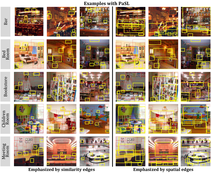
Figure 3: Visualization of PaSL. We choose some examples with PaSL from five scene categories. Each example shows the image with 32 rectangles representing the local regions in PaSL. For better visualization, we sort all 32 local regions and emphasize the top 8 regions in yellow and thick rectangles and downplay other regions in red and thin rectangles. The left 3 columns show the images with the regions emphasized by similarity edges. The right 3 columns show the same images with the regions emphasized by spatial edges. This figure is better viewed in color.

IV-C2 The Difference of PaSL

Although each image has its own spatial structure, PaSLs derived from the same pretrained model will have some similar properties. From the point of view of PaSLs in the whole training data, we define a metric named Coverage Ratio, which is the ratio between the coverage area of PaSL and the area of the image, to analyze the properties of PaSLs. In Fig. 4, the boxplots show the distributions of Coverage Ratio for all training image PaSLs derived from three different pretrained models. Note that the number of regions in PaSL is fixed to 32 for a fair comparison. We find that PaSLs derived from models pretrained on scene-centric datasets (Places205 or Places365) focus on larger regions compared to them derived from the model pretrained on object-centric dataset (ImageNet). And also PaSLs derived from the model pretrained on ImageNet may focus on the regions with high objectness. So, the values of their Coverage Ratio have a larger diversity due to the wide variety of size and location of objects in scene images.

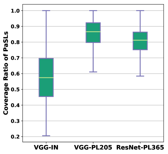
Figure 4: The distributions of Coverage Ratio of PaSLs derived from different pretrained models (VGG-IN, VGG-PL205, and ResNet-PL365). Coverage Ratio is the ratio between the coverage area of PaSL and the area of the image.

IV-C3 The Generalization of PaSL

Considering the independence between PaSL construction and LGN, we can explore the generalization of PaSL by combining PaSL with LGN when they are based on different or same pretrained models. There are three kinds of PaSLs derived from different pretrained models, and three kinds of LGNs based on different pretrained models. Therefore, we conduct combination experiments on MIT67, and report nine combination results in Table IV. When the pretrained models are different for PaSL and LGN, the performance can yield a change of no more than $1.04\%$. Besides different combination of PaSL and LGN, we also evaluate another spatial layout formed by regions generated by Faster RCNN [52] pretrained on MSCOCO dataset. For a fair comparison, we set the number of regions in this layout to 32. Based on Table IV, we can have three observations. 1) Compared to PaSLs derived from other pretrained models, the one from VGG-PL205 has the better ability to represent the spatial structure of scene images. 2) Despite having some fluctuations in performance, PaSLs derived from different pretrained models have comparable value for scene recognition, which demonstrates their considerable generalization capability. 3) The spatial layout generated by object detection obtains the worst performances with all LGNs. One possible reason is that this layout mainly focus on some common objects, and is not suitable to capture the complex structural layouts of scene images.

TABLE IV: The generalization of PaSLs derived from different pretrained models. We show classification accuracy (%) of the combinations of PaSL and LGN, when they are based on different or same pretrained models. The best result of each row is marked in bold.

LGN	PaSL			Detection
	VGG-IN	VGG-PL205	ResNet-PL365
VGG-IN	79.78	80.52	80.07	68.66
VGG-PL205	84.78	85.37	85.29	80.52
ResNet-PL365	88.21	88.73	87.69	83.66

IV-D Experimental Study of LGN

IV-D1 Configuration of Hyperparameters

Three hyperparameters are important to determine the performance of our method, the number of clusters $N$ in constructing PaSL, the hidden size $h_{1}$ in graph convolution, and the $\lambda$ in node weak-supervision mechanism. To investigate these three hyperparameters, we conduct several experiments on MIT67 dataset. Because the architectures of VGG16 and ResNet50 are different, especially the processes from the last convolutional layer to output prediction layer, we analyze these hyperparameters on VGG-PL205 and ResNet-PL365 pretrained models, separately. We do not show the analysis on VGG-IN, since it has a similar behavior with VGG-PL205.

We evaluate the effect of hidden size $h_{1}$ and the number of clusters $N$ on spatial subgraph without global information and node weak-supervision in Fig. 5. It can be observed that the trends of accuracy caused by hidden size $h_{1}$ are different with VGG-PL205 and ResNet-PL365. In Fig. 5 (a), the accuracy has a significant increment when hidden size $h_{1}$ is lower than 8192, and then tends to be stable as hidden size $h_{1}$ increases. However, in Fig. 5 (b), we can see that the accuracy has a slight change as hidden size $h_{1}$ changes. These differences can be attributed to the aggregation techniques for generating the global image representation in different CNNs. In VGG16, the local spatial features are concatenated to produce the global representations, while they are averagely pooled in ResNet. Thus, in LGN based on VGG-PL205, aggregating the local features need to substantially enlarge the projection dimension (hidden size $h_{1}$) to prevent the information loss from averagely pooling, but not for ResNet-PL365. For instance, the ratios of hidden size $h_{1}$ to input dimension $h_{0}$ are 16 and 4 for VGG-PL205 and ResNet-PL365, respectively.

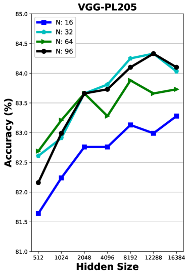
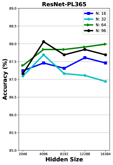
(a)	(b)

Figure 5: The effect of hidden size $h_{1}$ and the number of clusters $N$. We report the results on spatial subgraph without global information and node weak-supervision. Because of the architecture difference of VGG16 and ResNet50, we show the analysis results separately.

As illustrated in Fig. 5, when the number of clusters $N=32$, we obtain better performances by using VGG-PL205, and the similar observation can be found at $N=64$ with ResNet-PL365. Thus, we set hidden size and the number of clusters $\{h_{1},\thinspace N\}$ to $\{8192,\thinspace 32\}$ and $\{8192,\thinspace 64\}$ for VGG-PL205 and ResNet-PL365 respectively in all subsequent experiments. Besides $h_{1}$ and $N$, the hyperparameter $\lambda$ in node weak-supervision mechanism is also important. The node weak-supervision mechanism aims to force each local node to predict the image category, which makes local representations more specific for generating discriminative image representations. We report the results on spatial subgraph without global information for different values of $\lambda$ in Table V. It can be observed that, the best performances are obtained at $\lambda=4.0$ and $\lambda=1.0$ for VGG-PL205 and ResNet-PL365, respectively, which are set as default hyperparameters in subsequent experiments. We set the same hyperparameters $\{h_{1}=8192,\thinspace N=32,\thinspace\lambda=4.0\}$ for VGG-IN pretrained models.

TABLE V: The influence of $\lambda$ in node weak-supervision mechanism. We show the classification accuracy (%) based on spatial subgraph without global information. The best result of each row is marked in bold.

$\lambda$	0.0	1.0	2.0	3.0	4.0	5.0
VGG-PL205	84.25	84.18	84.18	84.32	84.55	84.40
ResNet-PL365	87.84	87.91	87.84	87.80	87.76	87.69

IV-D2 Effect of different subgraph combination methods

TABLE VI: A comparison of different subgraph combination methods without global information. Classification accuracy (%) is reported as evaluation metric. The best result of each column is marked in bold.

Method	VGG-PL205	ResNet-PL365
Addition	85.07	88.28
Maximum	84.93	88.13
Product	85.22	88.36

We perform a comparison of three different subgraph combination methods, e.g., element-wise addition, maximum and product. Table VI illustrates the results of LGN without global information on MIT67 dataset. The product combination method outperforms other methods. Compared to addition and maximum combination methods, the product method will produce more zero elements in output representations when the inputs are generated from the ReLU layer. This confirms that the sparsity of representation is helpful for the improvement of recognition performance.

TABLE VII: Ablation studies on MIT67. Classification accuracy (%) is reported as evaluation metric. The best result of each column is marked in bold.

Baseline	Spatial	Similarity	Global	Node	Pretrained Model
			Information	Weak-supervision	VGG-IN	VGG-PL205	ResNet-PL365
$\checkmark$	-	-	-	-	74.55	81.27	86.64
-	$\checkmark$	-	-	-	77.39	84.25	87.84
-	$\checkmark$	-	-	$\checkmark$	78.36	84.55	87.91
-	-	$\checkmark$	-	$\checkmark$	78.58	84.25	87.99
-	$\checkmark$	$\checkmark$	-	$\checkmark$	78.73	85.22	88.36
-	$\checkmark$	$\checkmark$	$\checkmark$	$\checkmark$	79.78	85.37	88.06
Improvement Over Baseline					5.23	4.1	1.42

IV-D3 Ablation Study

We conduct detailed ablation studies of our LGN on MIT67 dataset in Table VII. We analyze the effect of four components, two subgraphs, global information, and node weak-supervision mechanism across three different pretrained models. The $\ell_{2}$ normalized input representations of local regions are averagely pooled as the inputs to a linear SVM classifier, and then produce the classification results as baselines. In Table VII, the best results are marked in bold, which show the improvements of up to $\boldsymbol{5.23\%}$ over baselines. When applying node weak-supervision mechanism, LGN with VGG-IN has a better improvement. It can be attributed to the worse local representations for scene recognition. Moreover, it can be observed that the global information is useful for VGG16 pretrained models, but not for ResNet50 pretrained model. This may be caused by the better representations of local regions from ResNet-PL365 for capturing the whole image information. We also validate that the spatial and similarity subgraphs are both important to boost the performances and have similar improvements over the baselines. Furthermore, when combining these two subgraphs, there still have improvements, which demonstrates that the two subgraphs exist a complementary relation.

V Conclusion

We propose to construct Prototype-agnostic Scene Layout (PaSL) for each image, and introduce Layout Graph Network (LGN) to explore the spatial structure of PaSL for scene recognition. The pretrained CNN models can be used as region detectors to discover discriminative regions, then form PaSL for each image. To preserve the diverse and flexible spatial structures of PaSLs, we reform each PaSL as a layout graph where regions are defined as nodes and two kinds of independent relations between nodes are encoded as edges. Then, LGN applies graph convolution on the layout graph to integrate spatial and semantic similarity relations into image representations. The detailed ablation experiments demonstrate that LGN has a great ability to capture the spatial and similarity information in PaSL. With the qualitative and quantitative analyses, we prove that PaSLs can capture the useful and discriminative information of the images and have the considerable generalization capability. Experiments on three widely recognized datasets, MIT67, SUN397, and Places365, demonstrate that our approach can achieves superior performances in the setting of a single model in a single scale, and even obtains state-of-the-art results on MIT67 and SUN397.

In the future, we consider jointly learning scene layout and structural models, which may bring better optimization results. Another interesting direction is to explore the multi-scale information from different convolutional layers to help construct more precise and useful spatial structures of scene images.

References

- [1] A. Quattoni and A. Torralba, “Recognizing Indoor Scenes,” in CVPR, 2009, pp. 413–420. [Online]. Available: http://people.csail.mit.edu/torralba/publications/indoor.pdf
- [2] H. Izadinia, F. Sadeghi, and A. Farhadi, “Incorporating Scene Context and Object Layout into Appearance Modeling,” in CVPR. IEEE, 2014, pp. 232–239. [Online]. Available: http://ieeexplore.ieee.org/lpdocs/epic03/wrapper.htm?arnumber=6909431
- [3] Z. Zuo, B. Shuai, G. Wang, X. Liu, X. Wang, B. Wang, and Y. Chen, “Learning Contextual Dependence With Convolutional Hierarchical Recurrent Neural Networks,” IEEE Transactions on Image Processing, vol. 25, no. 7, pp. 2983–2996, jul 2016. [Online]. Available: http://ieeexplore.ieee.org/document/7442840/
- [4] R. Wu, B. Wang, and W. Wang, “Harvesting Discriminative Meta Objects with Deep CNN Features for Scene Classification,” in ICCV, 2015, pp. 1287–1295.
- [5] Z. Zhao and M. Larson, “From Volcano to Toyshop: Adaptive Discriminative Region Discovery for Scene Recognition,” in ACM MM, 2018. [Online]. Available: http://dx.doi.org/10.1145/3240508.3240698
- [6] Y. Liu, Q. Chen, W. Chen, and I. Wassell, “Dictionary Learning Inspired Deep Network for Scene Recognition,” in AAAI, 2018, pp. 7178–7185.
- [7] M. Pandey and S. Lazebnik, “Scene recognition and weakly supervised object localization with deformable part-based models,” in ICCV. IEEE, 2011, pp. 1307–1314. [Online]. Available: http://ieeexplore.ieee.org/document/6126383/
- [8] T. N. Kipf and M. Welling, “SEMI-SUPERVISED CLASSIFICATION WITH GRAPH CONVOLUTIONAL NETWORKS,” in ICLR, 2017. [Online]. Available: https://arxiv.org/pdf/1609.02907.pdf
- [9] D. Bau, B. Zhou, A. Khosla, A. Oliva, and A. Torralba, “Network Dissection: Quantifying Interpretability of Deep Visual Representations,” in CVPR. IEEE, 2017, pp. 3319–3327. [Online]. Available: http://ieeexplore.ieee.org/document/8099837/
- [10] X. Song, S. Jiang, and L. Herranz, “Multi-Scale Multi-Feature Context Modeling for Scene Recognition in the Semantic Manifold,” IEEE Transactions on Image Processing, vol. 26, no. 6, pp. 2721–2735, jun 2017. [Online]. Available: http://ieeexplore.ieee.org/document/7885099/
- [11] J. Xiao, J. Hays, K. Ehinger, A. Oliva, and A. Torralba, “SUN Database: Large Scale Scene Recognition from Abbey to Zoo,” in CVPR, 2010, pp. 3485–3492.
- [12] B. Zhou, A. Lapedriza, A. Khosla, A. Oliva, and A. Torralba, “Places: A 10 Million Image Database for Scene Recognition,” IEEE Transactions on Pattern Analysis and Machine Intelligence, vol. 40, no. 6, pp. 1452–1464, 2018.
- [13] H. Jegou, M. Douze, C. Schmid, and P. Perez, “Aggregating local descriptors into a compact image representation,” in CVPR. IEEE, 2010, pp. 3304–3311. [Online]. Available: http://ieeexplore.ieee.org/document/5540039/
- [14] F. Perronnin, J. Sánchez, and T. Mensink, “Improving the Fisher Kernel for Large-Scale Image Classification,” in ECCV, 2010, pp. 143–156. [Online]. Available: http://link.springer.com/10.1007/978-3-642-15561-1_11
- [15] D. G. Lowe, “Distinctive Image Features from Scale-Invariant Keypoints,” International Journal of Computer Vision, vol. 60, no. 2, pp. 91–110, 2004. [Online]. Available: https://www.cs.ubc.ca/~lowe/papers/ijcv04.pdf
- [16] S. Lazebnik, C. Schmid, J. Ponce, S. Lazebnik, C. Schmid, and J. Ponce, “Beyond Bags of Features : Spatial Pyramid Matching for Recognizing Natural Scene Categories,” in CVPR, 2006, pp. 2169–2178.
- [17] S. N. Parizi, J. G. Oberlin, and P. F. Felzenszwalb, “Reconfigurable Models for Scene Recognition,” in CVPR, 2012, pp. 2775–2782.
- [18] G. S. Xie, X. Y. Zhang, S. Yan, and C. L. Liu, “Hybrid CNN and Dictionary-Based Models for Scene Recognition and Domain Adaptation,” IEEE Transactions on Circuits and Systems for Video Technology, vol. 27, no. 6, pp. 1263–1274, 2017.
- [19] Y. Li, M. Dixit, and N. Vasconcelos, “Deep Scene Image Classification With the MFAFVNet,” in ICCV, 2017.
- [20] B. Chen, J. Li, G. Wei, and B. Ma, “A novel localized and second order feature coding network for image recognition,” Pattern Recognition, vol. 76, pp. 339–348, 2018.
- [21] S. Singh, A. Gupta, and A. A. Efros, “Unsupervised discovery of mid-level discriminative patches,” in ECCV, 2012, pp. 73–86. [Online]. Available: http://arxiv.org/abs/1205.3137
- [22] M. Juneja, A. Vedaldi, C. V. Jawahar, and A. Zisserman, “Blocks That Shout: Distinctive Parts for Scene Classification,” in CVPR, 2013, pp. 923–930.
- [23] X. Cheng, J. Lu, J. Feng, B. Yuan, and J. Zhou, “Scene recognition with objectness,” Pattern Recognition, vol. 74, pp. 474–487, 2018. [Online]. Available: https://doi.org/10.1016/j.patcog.2017.09.025
- [24] H. Zheng, J. Fu, T. Mei, and J. Luo, “Learning Multi-attention Convolutional Neural Network for Fine-Grained Image Recognition,” in ICCV. IEEE, oct 2017, pp. 5219–5227. [Online]. Available: http://ieeexplore.ieee.org/document/8237819/
- [25] X.-S. Wei, J.-H. Luo, J. Wu, and Z.-H. Zhou, “Selective Convolutional Descriptor Aggregation for Fine-Grained Image Retrieval,” IEEE Transactions on Image Processing, vol. 26, no. 6, pp. 2868–2881, jun 2017. [Online]. Available: http://ieeexplore.ieee.org/document/7887720/
- [26] F. Scarselli, M. Gori, A. C. Tsoi, M. Hagenbuchner, and G. Monfardini, “The graph neural network model.” IEEE Transactions on Neural Networks, vol. 20, no. 1, pp. 61–80, 2009.
- [27] Y. Li, D. Tarlow, M. Brockschmidt, and R. Zemel, “Gated Graph Sequence Neural Networks,” in ICLR, 2016. [Online]. Available: http://arxiv.org/abs/1511.05493
- [28] J. Gilmer, S. S. Schoenholz, P. F. Riley, O. Vinyals, and G. E. Dahl, “Neural Message Passing for Quantum Chemistry,” in ICML, 2017. [Online]. Available: http://arxiv.org/abs/1704.01212
- [29] K. Marino, R. Salakhutdinov, and A. Gupta, “The More You Know: Using Knowledge Graphs for Image Classification,” in CVPR, 2017. [Online]. Available: http://arxiv.org/abs/1612.04844
- [30] R. Li, M. Tapaswi, R. Liao, J. Jia, R. Urtasun, and S. Fidler, “Situation Recognition with Graph Neural Networks,” in ICCV, 2017, pp. 4183–4192. [Online]. Available: http://www.cs.utoronto.ca/~rjliao/papers/iccv_2017_situation.pdf
- [31] J. Yang, J. Lu, S. Lee, D. Batra, and D. Parikh, “Graph R-CNN for Scene Graph Generation,” in ECCV, 2018. [Online]. Available: http://arxiv.org/abs/1808.00191
- [32] X. Wang, Y. Ye, and A. Gupta, “Zero-shot Recognition via Semantic Embeddings and Knowledge Graphs,” in CVPR, 2018. [Online]. Available: http://arxiv.org/abs/1803.08035
- [33] A. T. Bolei Zhou, Aditya Khosla, Agata Lapedriza, Aude Oliva, “Object detectors emerge in deep scene CNNs,” in ICLR, 2015. [Online]. Available: http://arxiv.org/abs/1412.6856
- [34] B. Zhou, A. Lapedriza, J. Xiao, A. Torralba, and A. Oliva, “Learning Deep Features for Scene Recognition using Places Database,” in NIPS, 2014, pp. 487–495. [Online]. Available: http://papers.nips.cc/paper/5349-learning-deep-features-for-scene-recognition-using-places-database.pdf
- [35] S. Suzuki and K. Be, “Topological structural analysis of digitized binary images by border following,” Computer vision, graphics, and image processing, vol. 30, no. 1, pp. 32–46, apr 1985. [Online]. Available: http://linkinghub.elsevier.com/retrieve/pii/0734189X85900167
- [36] K. He, G. Gkioxari, P. Dollar, and R. Girshick, “Mask R-CNN,” in ICCV. IEEE, 2017, pp. 2980–2988. [Online]. Available: http://ieeexplore.ieee.org/document/8237584/
- [37] R. Yu, A. Li, V. I. Morariu, and L. S. Davis, “Visual Relationship Detection with Internal and External Linguistic Knowledge Distillation,” in ICCV. IEEE, 2017, pp. 1068–1076. [Online]. Available: http://ieeexplore.ieee.org/document/8237383/
- [38] Jia Deng, Wei Dong, R. Socher, Li-Jia Li, Kai Li, and Li Fei-Fei, “ImageNet: A large-scale hierarchical image database,” in CVPR, 2009, pp. 248–255. [Online]. Available: http://ieeexplore.ieee.org/lpdocs/epic03/wrapper.htm?arnumber=5206848
- [39] L. Herranz, S. Jiang, and X. Li, “Scene Recognition with CNNs: Objects, Scales and Dataset Bias,” in CVPR, 2016, pp. 571–579. [Online]. Available: http://ieeexplore.ieee.org/document/7780437/
- [40] J. L. Ba, J. R. Kiros, and G. E. Hinton, “Layer Normalization,” arXiv preprint, 2016. [Online]. Available: http://arxiv.org/abs/1607.06450
- [41] D. P. Kingma and J. Ba, “Adam: A Method for Stochastic Optimization,” arXiv preprint, 2014. [Online]. Available: http://arxiv.org/abs/1412.6980
- [42] X. Glorot and Y. Bengio, “Understanding the difficulty of training deep feedforward neural networks,” in Proceedings of the thirteenth international conference on artificial intelligence and statistics, 2010, pp. 249–256. [Online]. Available: http://proceedings.mlr.press/v9/glorot10a/glorot10a.pdf
- [43] M. D. Dixit and N. Vasconcelos, “Object based Scene Representations using Fisher Scores of Local Subspace Projections,” in NIPS, 2016, pp. 2811–2819.
- [44] L. Liu, P. Wang, C. Shen, L. Wang, A. V. D. Hengel, C. Wang, and H. T. Shen, “Compositional Model Based Fisher Vector Coding for Image Classification,” IEEE Transactions on Pattern Analysis and Machine Intelligence, vol. 39, no. 12, pp. 2335–2348, 2017.
- [45] R. Sicre, Y. Avrithis, E. Kijak, and F. Jurie, “Unsupervised part learning for visual recognition,” in CVPR, 2017, pp. 3116–3124. [Online]. Available: http://openaccess.thecvf.com/content_cvpr_2017/papers/Sicre_Unsupervised_Part_Learning_CVPR_2017_paper.pdf
- [46] S. H. Khan, M. Hayat, and F. Porikli, “Scene Categorization with Spectral Features,” in ICCV. IEEE, 2017, pp. 5639–5649. [Online]. Available: http://ieeexplore.ieee.org/document/8237863/
- [47] P. Koniusz and H. Zhang, “A Deeper Look at Power Normalizations,” in CVPR, 2018. [Online]. Available: http://openaccess.thecvf.com/content_cvpr_2018/papers/Koniusz_A_Deeper_Look_CVPR_2018_paper.pdf
- [48] M. Dixit, Y. Li, and N. Vasconcelos, “Semantic Fisher Scores for Task Transfer: Using Objects to Classify Scenes,” IEEE Transactions on Pattern Analysis and Machine Intelligence, vol. PP, no. 8, pp. 1–1, 2019. [Online]. Available: https://ieeexplore.ieee.org/document/8734016/
- [49] X. Jin, Y. Chen, J. Dong, J. Feng, and S. Yan, “Collaborative Layer-Wise Discriminative Learning in Deep Neural Networks,” in ECCV, 2016, pp. 733–749. [Online]. Available: http://link.springer.com/10.1007/978-3-319-46478-7_45
- [50] Y. Pan, Y. Xia, and D. Shen, “Foreground Fisher Vector: Encoding Class-Relevant Foreground to Improve Image Classification,” IEEE Transactions on Image Processing, vol. 28, no. 10, pp. 4716–4729, oct 2019. [Online]. Available: https://ieeexplore.ieee.org/document/8678832/
- [51] L. Wang, S. Guo, W. Huang, Y. Xiong, and Y. Qiao, “Knowledge Guided Disambiguation for Large-Scale Scene Classification With Multi-Resolution CNNs,” IEEE Transactions on Image Processing, vol. 26, no. 4, pp. 2055–2068, 2017.
- [52] S. Ren, K. He, R. Girshick, and J. Sun, “Faster R-CNN: Towards Real-Time Object Detection with Region Proposal Networks,” IEEE Transactions on Pattern Analysis and Machine Intelligence, vol. 39, no. 6, pp. 1137–1149, jun 2017. [Online]. Available: http://ieeexplore.ieee.org/document/7485869/