HeteSpaceyWalk: A Heterogeneous Spacey Random Walk for Heterogeneous Information Network Embedding

Abstract.

Heterogeneous information network (HIN) embedding has gained increasing interests recently. However, the current way of random-walk based HIN embedding methods have paid few attention to the higher-order Markov chain nature of meta-path guided random walks, especially to the stationarity issue. In this paper, we systematically formalize the meta-path guided random walk as a higher-order Markov chain process, and present a heterogeneous personalized spacey random walk to efficiently and effectively attain the expected stationary distribution among nodes. Then we propose a generalized scalable framework to leverage the heterogeneous personalized spacey random walk to learn embeddings for multiple types of nodes in an HIN guided by a meta-path, a meta-graph, and a meta-schema respectively. We conduct extensive experiments in several heterogeneous networks and demonstrate that our methods substantially outperform the existing state-of-the-art network embedding algorithms.

1. Introduction

Heterogeneous Information Networks (HINs) have been studied for several years and proven to be useful for many applications (Shi et al., 2017; Cai et al., 2018). The heterogeneous information provided by the types of entities and their relationships in HINs can capture more semantically meaningful information than homogeneous networks (Sun et al., 2011). For example, consider a scholar network, as illustrated in Figure 1, which consists of three entity types: Author, Paper, and Venue, and two relationships: an author writes a paper, and a paper is published in a conference venue. We can introduce two meta-paths (Sun et al., 2011): “Author–Paper–Author (APA)” and “Author–Paper–Venue–Paper–Author (APVPA)” which measure the similarity of two authors who co-author many papers or whose papers are published at the same venues. The semantics of the two meta-paths give two specific definitions about how the two authors are seen as similar. Many HIN-specific applications, such as entity typing (Ren et al., 2015a; Ren et al., 2015b), similarity search (Sun et al., 2011, 2012), and link prediction (Yu et al., 2014; Zhao et al., 2017; Hu et al., 2018), have been applied to use the semantics of different meta-paths in HINs and have been shown to be useful.

Recently, inspired by the DeepWalk algorithm for homogeneous networks (Perozzi et al., 2014), meta-path(s) guided random walk based HIN embedding algorithms have also been developed (Dong et al., 2017; Fu et al., 2017; Shi et al., 2018a; Zhang et al., 2018b). In general, these algorithms use a two-step approach to generate node embeddings. First, they perform random walks on an HIN guided by one or mutiple meta-path(s). Then they run a Skipgram algorithm which was invented in word embedding approach word2vec (Mikolov et al., 2013b) to generate the node embeddings. The idea of Skipgram algorithm is to use a central node to predict its context nodes given by the random-walk paths. Despite their success in capturing the heterogeneous information provided by meta-paths and thus learning valuable embedding vectors, there are still some problems. First, the meta-path guided random walk uses sampling to generate node paths, which are in essence sampled from a higher-order Markov chain. For example, as illustrated in Figure 1, for the random walks guided by the meta-path “APVPA”, we will constrain that for the first “P” in the meta-path, the next node must be “V” and for the second “P” in the meta-path, the next node must be “A”. That is, when we perform next walk from a “P”, we need to know the previous state before “P” being “A” or “V” to judge the “P” being the first or the second. Thus, this is theoretically a second-order Markovian stochastic process. However, existing algorithms have paid few attention to the essence of the higher-order Markov chain property of meta-path guided random walk, especially to its limiting stationary distribution. As a random walk can be regarded as a random sampling from the stationary distribution, their inattentive sampling may result in less accurate approximation of the stationary distribution and consequently may have less effective node embeddings. Second, compared with single meta-path, meta-graph is able to capture richer information by integrating multiple meta-paths. However, as different meta-paths characterize different semantics, it is still a challenge how to effectively select and balance multiple meta-paths with appropriate weights. Moreover, the design of meta-paths is usually domain-specific and is difficult for a non-proficient user. Thus, a more principled way of performing HIN embedding should be fit to extend to a general meta-schema driven embedding model for when proficient design is impracticable.

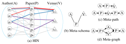
Figure 1. An illustrative heterogeneous scholar network with three entity types: Author(A), Paper(P), and Venue(V), as well as its meta-schema and some meta-paths/meta-graphs on the meta-schema.

In this paper, to address the above issues, first, we systematically clarify that the meta-path guided random walk is a higher-order Markov chain process. Then a meta-path based heterogeneous personalized spacey random walk (called HeteSpaceyWalk) is introduced to improve the walk effectiveness and efficiency by leveraging a non-Markovian spacey strategy. Given an arbitrary meta-path, instead of strictly constraining the walks by the meta-path, the HeteSpaceyWalk allows spacing out and skipping the intermediate trivial transitions, and in fact performs a special meta-graph guided random walk, which differs from the normal one in four aspects: (a) The special meta-graph integrates multiple meta-paths which are automatically produced by folding the original user-given meta-path. (b) The trade-off of these integrated meta-paths are dynamically self-adjusted. That is, during the walk process, HeteSpaceyWalk adaptively adjusts the probability of following each possible meta-path according to the carefully designed personalized spacey strategy. (c) HeteSpaceyWalk is mathematically guaranteed to attain the same unique limiting stationary distribution with the original meta-path guided higher-order Markovian random walk. (d) By spacing out and skipping the intermediate trivial transitions, HeteSpaceyWalk provides a cost-efficient sampling way to be stationary and thus can produce more effective embeddings with less walk-times and walk-length than original meta-path constrained random walk sampling.

Second, by leveraging the HeteSpaceyWalk process to generate heterogeneous neighborhood, and incorporating them to the Skipgram model, we develop a general scalable HIN embedding algorithm: SpaceyMetapath, which is able to produce semantically meaningful embeddings for multi-typed nodes in an HIN with an arbitrary user-given meta-path. Further, we extend the guidance from a single meta-path to a user-given meta-graph and a general non-handcrafted meta-schema, and develop two embedding algorithms: SpaceyMetagraph and SpaceyMetaschema. The main contributions of our work are summarized as follows:

$\bullet$ Existing approaches have paid few attention to the higher-order Markov chain nature of meta-path guided random walk, especially to its stationary distribution. We formalize the meta-path guided random walk as a higher-order Markov chain process, and present a heterogeneous personalized spacey random walk to efficiently and effectively attain the expected stationary distribution among nodes, which is based on a solid mathematical foundation (Benson et al., 2017).

$\bullet$ We propose a generalized framework for heterogeneous spacey random walk for a meta-path based higher-order Markov chain for HIN embeddings. Based on this framework, we further extend to an arbitrary meta-graph integrating multiple meta-paths and a general meta-schema without any handcrafted meta-paths.

$\bullet$ We use extensive experiments in four heterogeneous networks to demonstrate that the proposed methods considerably outperform both conventional homogeneous embedding and heterogeneous meta-path/meta-graph guided embedding methods in two HIN mining tasks, i.e., node classification and link prediction.

The code is available at https://github.com/HKUST-KnowComp/HeteSpaceyWalk.

2. Problem Definition

In this section, we introduce the formulation of the heterogeneous information network embedding problem. We first define several key concepts related to HINs as follows (Sun and Han, 2012).

Definition 2.1.

Heterogeneous Information Network (HIN). An information network is defined as a directed graph ${\mathcal{G}}=({\mathcal{V}},{\mathcal{E}})$ with an entity type mapping $\phi$: ${\mathcal{V}}\to\mathcal{A}$ and a relation type mapping $\psi$: ${\mathcal{E}}\to\mathcal{R}$, where ${\mathcal{V}}$ denotes the entity set, ${\mathcal{E}}$ denotes the relation set, $\mathcal{A}$ denotes the entity type set, and $\mathcal{R}$ denotes the relation type set. When the number of entity types $|\mathcal{A}|>1$ or the number of relation types $|\mathcal{R}|>1$, the network is called a heterogeneous information network. Otherwise, it is called a homogeneous information network.

The meta-schema (or network-schema) provides a high-level description of a given heterogeneous information network.

Definition 2.2.

Meta-schema. Given an HIN ${\mathcal{G}}=({\mathcal{V}},{\mathcal{E}})$ with the entity type mapping $\phi$: ${\mathcal{V}}\to\mathcal{A}$ and the relation type mapping $\psi$: $\mathcal{E}\to\mathcal{R}$, the meta-schema (or network-schema) for network $\mathcal{G}$, denoted as $\mathcal{T}_{\mathcal{G}}=(\mathcal{A},\mathcal{R})$, is a graph with entity types as nodes from $\mathcal{A}$ and relation types as edges from $\mathcal{R}$.

Another important concept is the meta-path (Sun et al., 2011) which defines relationships between entities at the schema level.

Definition 2.3.

Meta-path. A meta-path $\mathcal{P}$ is a path defined on the graph of meta-schema $\mathcal{T}_{\mathcal{G}}=(\mathcal{A},\mathcal{R})$, with the form of a sequence of node types $\it A_{1},A_{2},...,A_{L+1}$ and/or relation types $\it R_{1},R_{2},...,R_{L}$: ${\it A_{1}\xrightarrow{R_{1}}A_{2}\xrightarrow{R_{2}}\dots\xrightarrow{R_{L}}A_{L+1}}$ (or $\mathcal{P}={\it(A_{1}\to A_{2}\to\ldots\to A_{L+1})}$ when there is no ambiguity), which defines a composite relation $R=R_{1}\cdot R_{2}\cdot\ldots\cdot R_{L}$ between types $A_{1}$ and $A_{L+1}$, where $\cdot$ denotes relation composition operator, and $L$ is the length of $\mathcal{P}$.

We call a path $p\!=\!(v_{1}\!\to\!v_{2}\!\to\!\ldots\!\to\!v_{L+1})$ between $v_{1}$ and $v_{L+1}$ in network $\mathcal{G}$ follows the meta-path $\mathcal{P}$, if $\forall l,\phi(v_{l})\!=\!A_{l}$ and each edge $e_{l}\!=\!\langle v_{l},v_{l+1}\rangle$ belongs to each relation type $R_{l}$ in $\mathcal{P}$. We call $p$ as a path instance of $\mathcal{P}$, denoted as $p\!\in\!\mathcal{P}$. Besides the meta-path, the meta-graph (or meta-structure) is also very useful which captures complex semantics by integrating multiple meta-paths  (Fang et al., 2016; Huang et al., 2016).

Definition 2.4.

Meta-graph. A meta-graph (or meta-structure) is a directed acyclic graph $\mathcal{T}_{\mathcal{S}}\!=\!(\mathcal{A}_{S},\mathcal{R}_{S})$ defined on the given HIN schema $\mathcal{T}_{\mathcal{G}}\!=\!(\mathcal{A},\mathcal{R})$, where ${\mathcal{A}_{S}}\!\subseteq\!{\mathcal{A}}$ and ${\mathcal{R}_{S}}\!\subseteq\!{\mathcal{R}}$. In general, a meta-graph has only a single source entity type $A_{s}$ (i.e., with 0 in-degree) and a single target entity type $A_{t}$ (i.e., with 0 out-degree). Specially, we call the meta-graph $\mathcal{T}_{\mathcal{S}}$ with $A_{s}\!=\!A_{t}$ as a recursive meta-graph because it can be recursively extended by tail-head concatenation.

As an illustration, Figure 1 shows a heterogeneous network and its meta-schema, as well as the meta-paths and meta-graphs defined at the schema level. Finally, by considering an HIN as an input, we formally define the problem of HIN embedding as follows.

Definition 2.5.

Heterogeneous Information Network Embedding. Given a heterogeneous information network, denoted as a graph ${\mathcal{G}}=({\mathcal{V}},{\mathcal{E}};\mathcal{A},\mathcal{R})$. Embedding is to learn a function ${\mathnormal{f}}:{\mathcal{V}}\to{\mathbb{R}}^{d}$ that projects each node $v\in{\mathcal{V}}$ to a vector in a d-dimensional latent space ${\mathbb{R}}^{d}$, $d\ll|{\mathcal{V}}|$ that are able to capture the structures and semantics of multiple types of nodes and relationships.

3. Heterogeneous Spacey Random Walk based Embeddings

In this section, we introduce the general HIN embedding frameworks for a meta-path, a meta-graph, and a meta-schema.

3.1. Meta-path based HIN Embedding

Given an arbitrary meta-path $\mathcal{P}\!=\!{\it(A_{1}\!\to\!A_{2}\!\to\!\ldots\!\to\!A_{L\!+\!1})}$, our goal is to learn the semantically meaningful embeddings for all entities under the constraint of $\mathcal{P}$. We proceed by extending the meta-path guided random walk based embedding (Dong et al., 2017) in view of the scalability for large-scale networks.

3.1.1. Background of Random Walk over HIN

Meta-path guided random walk over an HIN was first considered in computing similarities in the path ranking algorithm (PRA) (Lao and Cohen, 2010). It defines the following transition probabilities:

(1) $${\bf P}_{\!A_{l},A_{l+1}}={\bf D}_{\!A_{l},A_{l+1}}^{-1}{\bf W}_{\!A_{l},A_{l+1}},$$

where ${\bf W\!}_{\!A_{l}\!,A_{l+1}}$ is the adjacency matrix between nodes in type $A_{l}$ and nodes in type $A_{l+1}$, and ${\bf D\!}_{\!A_{l},A_{l+1}}$ is the degree matrix with ${\bf D\!}_{\!A_{l},A_{l+1}}\!(v_{i},\!v_{i})\!\!=\!\!\!\sum_{j}\!\!{\bf W\!}_{\!A_{l}\!,A_{l+1}}\!(v_{i},\!v_{j})$. When performing a random walk from a node $v_{i}$ in type $A_{l}$, we choose next node $v_{j}$ in type $A_{l+1}$ based on the probability ${\bf P}_{\!A_{l},A_{l+1}}(\!v_{i},\!v_{j})$. In PRA algorithm, it uses the normalized commuting matrix, i.e., ${\bf P\!}_{\!A_{1}\!,A_{2}}\!\!\cdot\!{\bf P\!}_{\!A_{2}\!,A_{3}}\!\!\cdot\!\ldots\!\cdot\!{\bf P\!}_{\!A_{\!L}A_{\!L+1}}$ to define the meta-path based similarities between nodes of type $A_{1}$ and $A_{L+1}$, and claims that this is an ad-hoc definition of hitting/commuting probability. The actual expected hitting/commuting probability can be approximated by the stationary distribution of the random walk following the meta-path constraints. However, as discussed in Section 1, the existing random walk based HIN embedding methods (e.g., (Dong et al., 2017; Fu et al., 2017; Shi et al., 2018a; Zhang et al., 2018b)) directly use the random walk sampling but pay few attention to definitely explore the higher-order Markov chain property of meta-path guided random walk, especially to its limiting stationary distribution, which is essential for describing the long-run behavior of the random walk.

3.1.2. Higher-order Markov Chains

In this section, we first clarify that the meta-path guided random walk is a higher-order Markov chain using the following lemma and its explanations.

Lemma 3.1.

For an arbitrary meta-path $\mathcal{P}\!=\!{\it(A_{1}\!\to\!A_{2}\!\to\!\cdots\!\to\!A_{\!L+\!1})}$, we can define a $k$th-order Markov chain, iff $\mathcal{P}$ can be divided into a set of unique $k$-length meta-paths ${\it(\!A_{l}\!\to\!A_{l+1}\!\to\!\cdots\!\to\!A_{l+\!k})}$ which satisfy that if the last $k$ states are determined by ${\it(A_{l},A_{l+\!1},\cdots\!,A_{l+\!k-\!1})}$, the current state can only be $A_{l+k}$. After that, we can obtain the transition probabilities of the $k$th-order Markov chain by concatenating the normalized commuting/adjacency matrix of these $k$-length meta-paths, and such transition probabilities can be used to guide a random walk constrained by $\mathcal{P}$.

Note that to ensure the random walk runs continuously, we generally regard $\mathcal{P}$ should be cyclic with the same start and end entity types, i.e., $A_{1}\!=\!A_{L+1}$ (If not, it is easy to jump back from either start or end to get a symmetric one). Taking the meta-path “APVPA” illustrated in Figure 1 as an example, we can divide “APVPA” into a set of meta-paths: “APV”, “PVP”, “VPA”, and “PAP”. With these factorized meta-paths, walking to the current state is uniquely determined by the last two states. For example, if and only if the last state is a paper (P) and the second last state is an author (A), the current state can be only determined to be a venue (V). Thus a second-order Markov chain can be used to represent the “APVPA” guided random walk. Further, we can define a hypermatrix (three-dimensional tensor) to denote the transition probability for such second-order Markovian random walk.

Definition 3.2.

A second-order hypermatrix ${\bf H}$ for the meta-path guided second-order Markovian random walk can be defined as:

(2) $${\bf H}_{i,j,k}\triangleq\left\{\begin{aligned} &\phi(v_{i})=A_{l},\\ {\bf P}_{A_{l+1},A_{l+2}}(v_{j},v_{k}),\ \ \ &\phi(v_{j})=A_{l+1}\\ &\phi(v_{k})=A_{l+2}\\ 0,otherwise&\end{aligned}\right.,$$

where ${\bf H}_{i,j,k}$ represents the transition probability to node $v_{k}$, given the last node $v_{j}$ and the second last node $v_{i}$; “$A_{l}A_{l+1}A_{l+2}$” is one of “APV”, “PVP”, “VPA”, or “PAP”; $\phi(\cdot)$ is the node type mapping; and ${\bf P}_{A_{l+1},A_{l+2}}$ is defined as Eq. (1).

Although we have formalized the meta-path guided higher-order Markovian random walk, there can be some trivial walks. Due to the nature of higher-order Markov chain, the transitions following a meta-path usually depend on the last several states rather than just the last one. As a result, an entity may play a redundant role in the walks. For example, we define the meta-path “APVPA” based second-order Markovian random walk to extract the author similarity by the semantic “Two authors published at a venue”, and the walk path instances are illustrated in Figure 1(a). Among them, we can find the red one $a_{1}\!\!\to\!\!p_{1}\!\!\to\!\!v_{1}\!\!\to\!\!p_{1}\!\!\to\!\!a_{2}$ actually expresses the same information as the path instance $a_{1}\!\!\to\!\!p_{1}\!\!\to\!\!a_{2}$ following “APA”. In this case, the intermediate transitions $p_{1}\!\!\to\!\!v_{1}\!\!\to\!\!p_{1}$ are trivial walks and can be skipped, i.e., when we walked from an author $a_{1}$ to a paper $p_{1}$, we then can immediately skip to another author as if the current $p_{1}$ was just walked from a venue $v_{1}$. Such shortened walk path $a_{1}\!\!\to\!\!p_{1}\!\!\to\!\!a_{2}$ can be regarded as a faster instance of meta-path “APVPA”. This fact motivates us that instead of strictly constraining the walks by the meta-path, it can be preferred to occasionally skip the intermediate trivial transitions with a principled probability. Then, the meta-path based higher-order Markovian random walk can be more efficient to attain the expected stationary distribution. Intuitively, for any meta-path $\mathcal{P}^{*}\!\!=\!{\it(A_{1}\!\to\!\cdots\!A_{l}\!\to\!\cdots\!A_{k}\!\cdots\!\to\!\!A_{\!L+\!1})}$ with $A_{l}\!=\!A_{k}$, we can probabilistically perform a faster random walk following the folded meta-path ${\it(A_{1}\!\to\!\cdots\!A_{l}\!\to\!A_{k+\!1}\!\cdots\!\to\!A_{\!L+\!1})}$, and the walk path can be equivalently regarded as a special instance of meta-path $\mathcal{P}^{*}$. To achieve this, we introduce the following spacey random walk strategy.

3.1.3. Heterogeneous Personalized Spacey Random Walk

Given a higher-order Markov chain, the spacey random walk provides a space-friendly and efficient alternative approximation and is mathematically guaranteed to converge to the same limiting stationary distribution (Li and Ng, 2014; Benson et al., 2017). Inspired by that, to obtain the embeddings of multi-typed entities in an HIN, we first define our meta-path based heterogeneous personalized spacey random walk (called HeteSpaceyWalk) as follows. We use the aforementioned “APVPA” based second-order Markov chain and transition hypermatrix ${\bf H}_{i,j,k}$ as an illustration, while higher-order chains are similar.

Definition 3.3.

Heterogeneous Personalized Spacey Random Walk for a Meta-path based Second-order Markov Chain. Given a second-order Markov chain, the transition hypermatrix ${\bf H}_{i,j,k}$ is concatenated by a set of transition probabilities based on a set of factorized meta-paths (as defined in Eq. (2)). Then, these transition probabilities can be used to guide a personalized spacey random walk. Such stochastic process consists of a sequence of states/nodes $X(0),X(1),X(2),\cdots\!,X(n)$, and the probability law is defined to use

(3) $$Pr\!\left\{Y(n)\!=\!v_{i}|\mathcal{F}_{n}\right\}\triangleq\begin{cases}(1-\alpha)+\alpha{\bf w}_{i}(n),&v_{i}=X(n-1)\\ \alpha{\bf w}_{i}(n),&v_{i}\not=X(n-1)\end{cases}$$

to choose the second last state $Y(n)$, and then use

(4) $$Pr\!\left\{X(n+1)=v_{k}|X(n)=v_{j},Y(n)=v_{i}\right\}\triangleq{\bf H}_{i,j,k}$$

to choose the next node, where $\mathcal{F}_{n}$ is the $\sigma$-field generated by the random variables $X(i),i\!=\!1,2,...,n$, $X(0)$ is the initial state; $\alpha\in(0,1)$ is a hyper-parameter that can control a user’s personalized behavior; ${\bf w}(n)$ is the occupation vector at step $n$ and is defined as:

(5) $${\bf w}_{i}(n)\triangleq\frac{1}{n+N}\left(1+\sum_{s=1}^{n}Ind\left\{X(s)=v_{i}\right\}\right),$$

where $N$ is the number of total states.

In short, with personalization, once the spacey random walker visits $X(n)$ at step $n$, it spaces out and forgets its second last state (i.e., the state $X(n-1)$) with probability $\alpha$. It then invents a new history state $Y(n)$ by randomly drawing a past state $X(1),...,X(n)$. Then it transitions to $X(n+1)$ as if its last two states were $X(n)$ and $Y(n)$. Without personalization (i.e. $\alpha\!=\!0$), the spacey random walker performs a normal second-order Markovian random walk.

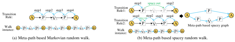
Figure 2. An intuitive comparison of meta-path based Markovian random walk and spacey random walk. When the spacey random walker walks from “P” to the next, it forgets its second last state is “A” and uses Eq. (3) to choose a new state which is assumed as the precursor of “P”. Constrained by “APVPA” based second-order Markov chain, the assumed precursor of “P” can be “V” or “A”, and respectively, there are two rules to guide the next transition: directly walk to “A” (rule1), or walk to “V” as a normal Markovian random walk (rule2).

Figure 2 shows an intuitive example of comparing normal meta-path based Markovian random walk and our proposed meta-path based spacey random walk, given the meta-path “APVPA” on the scholar network illustrated in Figure 1(a). We can see that, different from the Markovian random walk which strictly follows the constraints of the user-given meta-path, the spacey random walk allows skipping the intermediate transitions to improve walk efficiency and quality, which is actually a shortened random walk following the folded sub-path of the original user-given meta-path. In fact, as illustrated in Figure 2(b), the spacey strategy produces a special meta-graph/multi-meta-paths (which we call as the meta-path based spacey graph integrating the original user given meta-path and its folded sub-meta-paths) guided random walk process. As a result, the proposed spacey random walk can efficiently and effectively capture richer information and thus achieve better performance than the normal Markovian random walk. For example, we can see the two walk instances in Figure 2, which indicate that the spacey random walk can use shorter walk steps to capture richer relationships than normal Markovian random walk. Moreover, different from directly deploying meta-graph/multi-meta-paths guided random walk, which is problematic to determine appropriate proportions to balance multiple meta-paths, the proposed spacey random walk adaptively adjusts the probability of following the original meta-path or any folded sub-meta-path according to a carefully designed personalized occupation probability (as defined in Eq. (3)) calculated dynamically by past states. The following theorem shows the guarantee of only more efficiently and effectively extracting the specific semantic of domain-proficient meta-path provided by users, i.e., the proposed spacey strategy will not absorb other heterogeneous information beyond the users’ concern.

Theorem 3.4.

The limiting distribution of the heterogeneous personalized spacey random walk for a meta-path equals to the same stationary distribution of the original meta-path based higher-order Markovian random walk under the rank-one approximation condition.

The proof follows the spacey random walk theory (Benson et al., 2017) and $z$ eigenvector solution theory (Li and Ng, 2014) which point out that by considering a “rank-one approximation” for a transition hypermatrix ${\bf H}$ of second-order Markov chain, the stationary distribution formula reduces to

(6) $${\bf\pi}_{k}=\sum_{i,j}{\bf H}_{i,j,k}{\bf\pi}_{j}{\bf\pi}_{i},\ \ \sum_{k}{\bf\pi}_{k}=1,{\bf\pi}_{k}\geq 0,N\geq k\geq 1,$$

where ${\bf\pi}_{k}$ is node distribution and $N$ is the number of nodes. Following this, we next demonstrate that the unique stationary solution of meta-path based second-order Markov chain is also the limiting distribution of the proposed personalized spacey random walk.

First, we can formally express that the defined spacey random walker $\{X(n)\}$ approximates a second-order Markov chain with a first-order transition probability matrix:

(7) $$\begin{split}{\bf R}_{j,k}&\triangleq\sum_{i}{\bf H}_{i,j,k}\left((1-\alpha){\bf x}_{i}(n)+\alpha{\bf w}_{i}(n)\right)\\ &=[{\bf H}\cdot(((1-\alpha){\bf x}(n)+\alpha{\bf w}(n))\otimes{\bf I})]_{j,k},\end{split}$$

where ${\bf x}(n)$ is the nodes distribution at step $n$, ${\bf w}(n)$ is the occupation probability vector at step $n$ (as defined in Eq. (5)).

Then, if the process $\{X(n)\}$ converges to a unique stationary distribution ${\bf x}(n)$ satisfying ${\bf R}{\bf x}(n)={\bf x}(n)$, for the case $n\gg L>0$, we have:

$${\bf w}(n+L)\thickapprox\frac{n{\bf w}(n)+L{\bf x}(n)}{n+L}={\bf w}(n)+\frac{L}{n+L}({\bf x}(n)-{\bf w}(n)).$$

In a continuous time limit $L\to 0$, we have:

$$\frac{d{\bf w}(n)}{dL}\thickapprox\lim_{L\to 0}\frac{{\bf w}(n+L)-{\bf w}(n)}{L}=\frac{1}{n}({\bf x}(n)-{\bf w}(n)).$$

Thus, if this process converges, it must converge to a point where ${\bf x}(n)={\bf w}(n)$. Further, we can find that the limiting distribution ${\bf x}$ heuristically satisfy:

$${\bf x}={\bf R}{\bf x}={\bf H}\cdot({((1-\alpha){\bf x}+\alpha{\bf w})}\otimes{\bf I}){\bf x}={\bf H}\cdot({\bf x}\otimes{\bf I}){\bf x}={\bf H}\cdot({\bf x}\otimes{\bf x}).$$

That is,

$${\bf x}_{k}=\sum_{i,j}{\bf H}_{i,j,k}{\bf x}_{j}{\bf x}_{i}.$$

Therefore, the limiting distribution of matrix ${\bf R}$ is also the unique stationary solution of hypermatrix ${\bf H}$. The defined heterogeneous personalized spacey random walk provides an efficient alternative approximation for the meta-path based higher-order Markovian random walk without changing the limiting stationarity.

3.1.4. Spacey Random Walk based Embedding

Now we can use the heterogeneous personalized spacey random walk to generate node sequences in an HIN, and then feed them to the Skipgram model (Mikolov et al., 2013a; Mikolov et al., 2013b) to learn node embeddings. We follow (Dong et al., 2017) to define the heterogeneous Skipgram model. Given the generated paths corpus $\mathcal{V_{P}}$ guided by meta-path $\mathcal{P}$, the model is to minimize following objective function:

(8) $$\mathop{\arg\min}_{\theta}\ -\sum_{v_{i}\in\mathcal{V_{P}}}\sum_{A\in\mathcal{A}}\sum_{v_{j}\in{\mathcal{N}}_{A}(v_{i})}\log Pr(v_{j}|v_{i},\theta),$$

where ${\mathcal{N}}_{A}(v_{i})$ denotes $v$’s neighborhood with type $A$. For each pair of entities $(v_{i},v_{j})$, their joint probability $Pr(v_{j}|v_{i},\theta)$ is commonly defined as such softmax function:

(9) $$Pr(v_{j}|v_{i},\theta)=\frac{\exp\{{\bf u}_{j}^{T}{\bf v}_{i}\}}{\sum_{j^{\prime}}\exp\{{\bf u}_{j^{\prime}}^{T}{\bf v}_{i}\}},$$

where ${\bf u}_{j}$ is the context vector of $v_{j}$ and ${\bf v}_{i}$ is the embedding vector of $v_{i}$. We also use the negative sampling technique (Mikolov et al., 2013b) for optimizing Eq. (8) which is modified as:

(10) $$\log\sigma({\bf u}_{j}^{T}{\bf v}_{i}\})+\sum_{1}^{m}\mathbb{E}_{v_{c}\thicksim P_{n}(v_{i})}\left[\log\sigma(-{\bf u}_{c}^{T}{\bf v}_{i}\})\right],$$

where $\sigma(x)\!=\!\frac{1}{1+\exp\{-x\}}$ and $P_{n}(v_{i})$ is the sampling distribution.

We call the above approach as SpaceyMetapath algorithm.

3.2. Meta-graph based HIN Embedding

In this section, we further propose a meta-graph based spacey random walk algorithm, named SpaceyMetagraph. Compared with single meta-path, a meta-graph can capture more complex heterogeneous structures and richer semantics by integrating multiple meta-paths. The challenge is how to concatenate these different higher-order Markov chains with appropriate proportions, i.e., how to balance the branch choices in a meta-graph. For example, for the meta-graph in Figure 1(d), when we need to perform random walk from the first “P” to its successors, there are two choices: “A” or “V”. Unlike a higher-order Markovian transition, this transition does not depend on any previous state. To deal with this issue, we extend our spacey random walk principle from choosing previous states to choosing the branch choices, and define our meta-graph based heterogeneous personalized spacey random walk as follows.

Definition 3.5.

Meta-graph based Heterogeneous Personalized Spacey Random Walk. Given $M$ second-order Markov chains based on a meta-graph $\mathcal{T}_{\mathcal{S}}=(\mathcal{A}_{S},\mathcal{R}_{S})$ integrating $M$ meta-paths, an integrated transition hypermatrix ${\bf\overline{H}}$ for this meta-graph is defined as:

(11) $${\bf\overline{H}}_{i,j,k}=\frac{1}{\sum_{m}Ind\{{\bf H}_{i,j,k}^{m}>0\}}\sum_{m}{\bf H}_{i,j,k}^{m},$$

where ${\bf H}^{m}$ is the transition probabilities of $m$-th Markov chain as defined in Eq. (2). Then, the probability law to guide the meta-graph based heterogeneous personalized spacey random walk is defined to use the personalized occupation probability (as defined in Eq. (3)) to choose the second last state $Y(n)$, and use

(12) $$Pr\!\{\Phi\!(n\!+\!1)\!\!=\!\!A|X\!(n)\!\!=\!\!v_{j},\!Y\!(n)\!\!=\!\!v_{i}\}\!\!\triangleq\!\!\begin{cases}\!(1\!\!-\!\!\alpha)\frac{1}{|\!N_{\!{\small\mathcal{T}_{\!\mathcal{S}}}}\!(v_{i}\!,\!v_{j})\!|}\!+\!\alpha{\bf z}_{\!A}\!(n),\!\!&\!\!A\!\!\in\!\!N_{\!\mathcal{T}_{\!\mathcal{S}}}\!(v_{i}\!,\!v_{j})\\ 0,&otherwise\end{cases}$$

to choose the next node type $\Phi(n+1)$, and then use

(13) $$Pr\!\left\{X\!(n\!\!+\!\!1)\!=\!v_{k}|X\!(n)\!=\!v_{j},Y\!(n)\!=\!v_{i},\Phi(n\!\!+\!\!1)\!=\!A\right\}\!\!\triangleq\!\!\begin{cases}{\bf\overline{H}}_{i,j,k},\!&\!\phi(v_{k})\!=\!A\\ 0,&\phi(v_{k})\!\not=\!A\end{cases}$$

to choose the next node, where $N_{\!{\small\mathcal{T}_{\!\mathcal{S}}}}\!(v_{i},\!v_{j})$ is the set of successor types of edge $(\phi(v_{i}),\phi(v_{j}))$ in $\mathcal{T}_{\!\mathcal{S}}$, $\phi(\cdot)$ is the node type mapping; ${\bf z}(n)$ is the partial occupation vector at step $n$:

(14) $${\bf z}_{\!A}(n)\triangleq\frac{\sum_{\phi(v_{i})=A}{\bf w}_{i}(n)}{\sum_{\phi(v_{i})\in N_{\!{\small\mathcal{T}_{\!\mathcal{S}}}}\!(X\!(n),\!Y\!(n))}{\bf w}_{i}(n)},\ \ A\!\!\in\!\!N_{\!\mathcal{T}_{\!\mathcal{S}}}\!(X\!(n),\!Y\!(n)).$$

In short, with personalization, when the meta-graph based spacey random walker visits $X(n)$ at step $n$, it first forgets its second last state (i.e., the state $X(n-1)$) with a probability $\alpha$ and invents a new history state $Y(n)$ by randomly drawing a past state $X(1),...,X(n)$. Next, if there are branched node types, it chooses the next type $\Phi(n+1)$ according to their history distribution with probability $\alpha$. Then it transitions to $X(n+1)$ as if its last two states were $X(n)$ and $Y(n)$ and current node type $\phi(X(n+1))$ is $\Phi(n+1)$. Without personalization, it performs a non-spacey random walk and randomly chooses the next one from branched node types.

We develop the SpaceyMetagraph algorithm by leveraging the meta-graph based personalized spacey random walk to generate heterogeneous neighborhood, and then incorporating them to the Skipgram model to produce effective HIN embeddings.

3.3. Meta-schema based HIN Embedding

Although the meta-path and meta-graph have proved to be useful to capture heterogeneous semantics in an HIN, it is quite difficult for a non-proficient user to design appropriate meta-paths or meta-graphs. Therefore, it is considerable to extend meta-path/meta-graph driven embedding algorithms to a general meta-schema driven embedding algorithm. Unlike a meta-path or a meta-graph, the meta-schema does not contain duplicate types. Thus, the meta-schema guided random walk is a first-order Markov chain and we do not need to space out to choose previous states. However, similar to the meta-graph guided random walk, there is a balance issue for branch choices in a meta-schema. Therefore, we follow the SpaceyMetagraph algorithm to formalize the meta-schema based heterogeneous personalized random walk as follows.

Definition 3.6.

Meta-schema based Heterogeneous Personalized Random Walk. Given an HIN ${\mathcal{G}}=({\mathcal{V}},{\mathcal{E}})$ and its meta-schema $\mathcal{T}_{\mathcal{G}}=(\mathcal{A},\mathcal{R})$, the transition probability matrix ${\bf P}_{A_{l},A_{k}}$ starting from type $A_{l}$ to type $A_{k}$ is defined similar as Eq. (1). Then, the probability law to guide the meta-schema based heterogeneous personalized random walk is defined to use

(15) $$Pr\!\{\Phi\!(n\!+\!1)\!\!=\!\!A|X\!(n)\!\!=\!\!v_{i}\}\!\!\triangleq\!\!\begin{cases}\!(1\!\!-\!\!\alpha)\frac{1}{|N_{\!{\small\mathcal{T}_{\!\mathcal{G}}}}\!(v_{i}\!)|}\!+\!\alpha{\bf z}_{\!A}\!(n),\!\!&\!\!A\!\!\in\!\!N_{\!\mathcal{T}_{\!\mathcal{G}}}\!(v_{i})\\ 0,&otherwise\end{cases}$$

to choose the next node type $\Phi(n+1)$, and then use

(16) $$Pr\!\left\{X\!(n\!\!+\!\!1)\!=\!v_{j}|X\!(n)\!=\!v_{i},\!\Phi(n\!\!+\!\!1)\!=\!\!A\right\}\!\!\triangleq\!\!\begin{cases}{\bf P}_{\!\phi\!(\!v_{i}\!),\!A}(v_{i},\!v_{j}),\!\!&\!\!\phi(v_{j})\!\!=\!\!A\\ 0,\!\!&\!\!\phi(v_{j})\!\!\not=\!\!A\end{cases}$$

to choose the next node, where $N_{\!{\small\mathcal{T}_{\!\mathcal{G}}}}\!(v_{i})$ is the set of adjacency types of $\phi(v_{i})$ in $\mathcal{T}_{\!\mathcal{G}}$; ${\bf z}(n)$ is the partial occupation vector at step $n$:

(17) $${\bf z}_{\!A}(n)\triangleq\frac{\sum_{\phi(v_{i})=A}{\bf w}_{i}(n)}{\sum_{\phi(v_{i})\in N_{\!{\small\mathcal{T}_{\!\mathcal{G}}}}\!(X\!(n))}{\bf w}_{i}(n)},\ \ A\!\!\in\!\!N_{\!\mathcal{T}_{\!\mathcal{G}}}\!(X\!(n)).$$

Note that the meta-schema based heterogeneous personalized spacey random walk is a special case of the meta-graph based one where the meta-graph only has first-order Markov chains. It is different from directly performing random walk on the HIN by treating it as a homogeneous graph, as it dynamically determines what is the type of next node and choose a random node under the chosen type. Given the random walk based node sequences, the Skipgram model can be used to learn embeddings as described in Section 3.1. We similarly denote this general framework as SpaceyMetaschema.

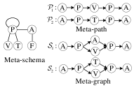
(a) ACM

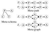
(b) DBLP

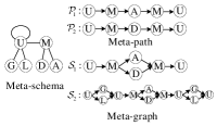
(c) Douban

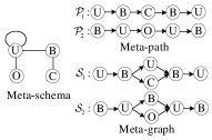
(d) Yelp

Figure 3. The meta-schema, meta-paths, and meta-graphs of each dataset used in the experiments.

4. Experiments

In this section, we show the experimental results.

4.1. Datasets

Here we use the following four heterogeneous networks:

$\bullet$ ACM: The ACM dataset (Shi et al., 2014) contains 196 venues (V), 12,499 papers (P), 1,533 terms (T), 17,431 authors (A), and 1,804 author affiliations (F). The meta-schema of ACM dataset is shown in Figure 3(a).

$\bullet$ DBLP: The dataset contains 14,376 papers (P), 20 conferences (C), 14,475 authors (A), and 8,920 terms (T). The meta-schema of DBLP dataset is shown in Figure 3(b).

$\bullet$ Douban: The Douban dataset (Shi et al., 2015) contains 13,367 users (U), 12,677 movies (M), 2,753 groups (G), 349 locations (L), 2,449 directors (D), and 6,311 actors (A). The meta-schema of Douban dataset is shown in Figure 3(c).

$\bullet$ Yelp: The Yelp dataset (Shi et al., 2015) contains 16,239 users (U), 14,284 businesses (B), 47 cities (C), and 11 compliments (O). The meta-schema of Yelp dataset is shown in Figure 3(d).

4.2. Experimental Settings

We compare the following state-of-the-art homogeneous and heterogeneous network embedding methods.

$\bullet$ DeepWalk (Perozzi et al., 2014) is a recently proposed homogeneous network embedding model, which learns $d$-dimensional node vectors by capturing the contextual information via uniform random walks.

$\bullet$ LINE (Tang et al., 2015b) is a method that preserves first-order and second-order proximities between nodes separately. We use the suggested version to learn two $d/2$-dimensional vectors (one for each-order) and then concatenate them.

$\bullet$ PTE (Tang et al., 2015a) is an extension of LINE for heterogeneous network embedding, which decomposes an HIN to a set of bipartite networks by edge types.

$\bullet$ Metapath2vec (Dong et al., 2017) is the current state-of-the-art network embedding method for HINs, which formalizes meta-path-based random walks to generate heterogeneous neighborhood and then leverages a heterogeneous skipgram model to perform node embeddings.

$\bullet$ Metagraph2vec (Zhang et al., 2018b) uses a meta-graph to guide the generation of random walks and to learn latent embeddings for multiple types of nodes in HINs.

We evaluate the quality of embedding vectors learned by different methods over two classical heterogeneous network mining tasks: multi-label node classification and link prediction. For the common hyperparameters, we set learning rate $lr\!=\!0.025$, negative samples $m\!=\!5$, and the embedding dimension $d\!=\!128$ for a trade-off between the computational time and accuracy. For random walk based methods, we set walk times per node $t\!=\!20$, walk length of each walk $l\!=\!320$, neighborhood size $w\!=\!10$. Specially, for our proposed SpaceyMetapath, SpaceyMetagraph, and SpaceyMetaschema, we set the personalized probability $\alpha\!=\!0.8$. For LINE and PTE, we set the total number of samples as 100 million. For meta-path driven (Metapath2vec, SpaceyMetapath) and meta-graph driven (Metagraph2vec, SpaceyMetagraph) methods, we survey most of the meta-path/meta-graph based work and empirically use some meta-paths and meta-graphs (which has been proven to be the most commonly effectively used schemes to extract heterogeneous semantics (Sun et al., 2011; Shi et al., 2014; Dong et al., 2017; Zheng et al., 2017; Zhang et al., 2018b)). The selected meta-paths and meta-graphs of each dataset are shown in Figure 3.

Table 1. The Micro-F1 scores for multi-label node classification. “–” indicates that the used meta-path/meta-graph cannot generate embeddings for nodes of target type.

Dataset	ACM			DBLP		Douban				Yelp
Node Type	Paper	Author	Venue	Paper	Author	User	Movie	Director	Actor	User	Business
DeepWalk	0.5746	0.5560	0.8198	0.6590	0.9231	0.7205	0.5606	0.6370	0.6592	0.5457	0.3393
LINE	0.5608	0.5887	0.8169	0.7120	0.9379	0.7431	0.5621	0.6396	0.6511	0.5324	0.3467
PTE	0.5613	0.5903	0.6838	0.6680	0.9368	0.7077	0.5595	0.5674	0.6260	0.5178	0.3360
Metapath2vec-$\mathcal{P}_{1}$	0.5774	0.6004	0.7826	0.8220	0.9397	0.7681	0.5678	–	0.6661	0.5585	0.3435
Metapath2vec-$\mathcal{P}_{2}$	0.5791	0.6164	–	0.5920	0.8627	0.7622	0.5454	0.6225	–	0.5648	0.2864
Metagraph2vec-$\mathcal{S}_{1}$	0.5688	0.6122	0.7880	0.8273	0.9365	0.7924	0.5842	0.6509	0.6669	0.6045	0.3529
Metagraph2vec-$\mathcal{S}_{2}$	0.6108	0.6486	0.7990	0.8076	0.9506	0.7953	0.5535	0.6115	0.6366	0.6012	0.3482
SpaceyMetapath-$\mathcal{P}_{1}$	0.5805	0.6140	0.8185	0.8410	0.9439	0.7864	0.5711	–	0.6839	0.6006	0.3574
SpaceyMetapath-$\mathcal{P}_{2}$	0.5880	0.6413	–	0.6300	0.8836	0.7768	0.5596	0.6368	–	0.5870	0.3312
SpaceyMetagraph-$\mathcal{S}_{1}$	0.5750	0.6171	0.8094	0.8520	0.9438	0.8036	0.5889	0.6676	0.6906	0.6101	0.3627
SpaceyMetagraph-$\mathcal{S}_{2}$	0.6136	0.6574	0.8412	0.8410	0.9521	0.8017	0.5720	0.6522	0.6809	0.6072	0.3524
SpaceyMetaschema	0.6145	0.6493	0.8369	0.8330	0.9512	0.8032	0.5793	0.6535	0.6832	0.5688	0.3536

Table 2. The Macro-F1 scores for multi-label node classification. “–” indicates that the used meta-path/meta-graph cannot generate embeddings for nodes of target type.

Dataset	ACM			DBLP		Douban				Yelp
Node Type	Paper	Author	Venue	Paper	Author	User	Movie	Director	Actor	User	Business
DeepWalk	0.1983	0.2403	0.3705	0.6504	0.9175	0.1789	0.3136	0.2408	0.2661	0.0584	0.1187
LINE	0.1891	0.2358	0.3649	0.6863	0.9238	0.2064	0.3120	0.2221	0.2382	0.0389	0.1164
PTE	0.1941	0.2474	0.3780	0.6376	0.9218	0.1687	0.2962	0.2279	0.2405	0.0314	0.1065
Metapath2vec-$\mathcal{P}_{1}$	0.1682	0.2408	0.4239	0.8073	0.9344	0.3703	0.2871	–	0.2732	0.0683	0.1147
Metapath2vec-$\mathcal{P}_{2}$	0.2019	0.3174	–	0.5110	0.8605	0.3288	0.2537	0.2305	–	0.0782	0.0609
Metagraph2vec-$\mathcal{S}_{1}$	0.1757	0.2973	0.4398	0.7988	0.9309	0.3958	0.3117	0.2571	0.2767	0.1362	0.1337
Metagraph2vec-$\mathcal{S}_{2}$	0.2113	0.3080	0.4254	0.7832	0.9462	0.3866	0.2606	0.2176	0.2351	0.1217	0.1263
SpaceyMetapath-$\mathcal{P}_{1}$	0.1797	0.2817	0.4518	0.8329	0.9399	0.3827	0.2921	–	0.3101	0.1297	0.1310
SpaceyMetapath-$\mathcal{P}_{2}$	0.2123	0.3571	–	0.5506	0.8774	0.3613	0.2767	0.2615	–	0.0968	0.1089
SpaceyMetagraph-$\mathcal{S}_{1}$	0.1862	0.3290	0.4616	0.8361	0.9363	0.4131	0.3154	0.2859	0.3247	0.1476	0.1431
SpaceyMetagraph-$\mathcal{S}_{2}$	0.2188	0.3511	0.4629	0.8243	0.9485	0.4015	0.2890	0.2678	0.3030	0.1270	0.1315
SpaceyMetaschema	0.2304	0.3587	0.4641	0.8196	0.9478	0.3827	0.3012	0.2699	0.3120	0.0768	0.1268

4.3. Multi-label Node Classification

For the node classification task, we first learn the node embedding vectors from the full nodes on each dataset, and then use the embeddings of the labeled nodes as input features for a one-vs-rest logistic regression classifier. We repeat each classification experiment ten times by randomly splitting 50% of the labeled nodes for training and the others for testing, and report the average performance in terms of both Micro-F1 score and Macro-F1 score. We also calculate the variances of the scores to reflect the significance of the experimental results.

We can observe that our proposed algorithms consistently outperform all the start-of-the-art baselines in both metrics on all datasets. For example, for the author node classification on the ACM dataset, our proposed models outperform all baseline models by around 0.01–0.10 (relatively 1%–18%) in terms of Micro-F1 scores and by around 0.04–0.12 (relatively 13%–52%) in terms of Macro-F1 scores. Moreover, given the same meta-path or meta-graph, the proposed SpaceyMetapath/SpaceyMetagraph imporves the author node classification performance by around 0.01–0.03 in Micro-F1 score and 0.03–0.04 in Macro-F1 score over Metapath2vec/Metagraph2vec.

In most cases, we can find that, by capturing the semantically meaningful information of an appropriate meta-path or meta-graph, the meta-path/meta-graph driven algorithms (including our proposed methods and Metapath2vec and Metagraph2vec) obviously outperform DeepWalk, LINE and PTE. Among them, meta-graph driven algorithms can achieve better performance than meta-path driven algorithms by capturing richer semantics of integrating multiple meta-paths. In addition, we can find that the proposed SpaceyMetaschema achieves competitive performance compared with the best of other methods, which may be more practical in complex networks with a large variety of types for the dispense with handcrafted domain-specific meta-paths/meta-graphs.

Table 3. Binary operators for learning edge features. The definitions correspond to the $i$-th component of vector ${\mathbf{u}}$ and ${\mathbf{v}}$.

Operator	Average	Hadamard	Weighted-L1	Weighted-L2
Definition	$({\mathbf{u}}_{i}+{\mathbf{v}}_{i})/2$	${\mathbf{u}}_{i}*{\mathbf{v}}_{i}$	$|{\mathbf{u}}_{i}-{\mathbf{v}}_{i}|$	${|{\mathbf{u}}_{i}-{\mathbf{v}}_{i}|}^{2}$

Table 4. The mean AUC scores for link prediction. “–” indicates that the used meta-path/meta-graph cannot generate embeddings for nodes of target type. The edge types for each dataset are shown in Figure 3.

Dataset	ACM			DBLP			Douban			Yelp
Edge Type	P–P	P–V	P–T	P–A	P–C	P–T	U–U	U–M	M–D	U–U	U–B	B–C
DeepWalk	0.8711	0.8775	0.6640	0.8743	0.9219	0.8777	0.6255	0.7906	0.8397	0.8768	0.8815	0.9212
LINE	0.8555	0.8550	0.6454	0.8180	0.8550	0.7479	0.6374	0.7850	0.8069	0.8770	0.8545	0.9063
PTE	0.6734	0.7189	0.5776	0.6410	0.7189	0.5901	0.6691	0.6461	0.5881	0.8319	0.7969	0.8244
Metapath2vec-$\mathcal{P}_{1}$	0.7137	0.9486	–	0.8801	0.9532	–	0.6061	0.7994	–	0.6464	0.8382	0.9179
Metapath2vec-$\mathcal{P}_{2}$	0.7392	–	0.7307	0.8848	–	0.8900	0.6006	0.8099	0.8793	0.7333	0.7841	–
Metagraph2vec-$\mathcal{S}_{1}$	0.7257	0.9393	–	0.8887	0.9438	–	0.6097	0.8081	0.8907	0.6493	0.8664	0.9081
Metagraph2vec-$\mathcal{S}_{2}$	0.7313	0.9467	0.6865	0.8925	0.9555	0.8765	0.6728	0.7711	0.8624	0.6919	0.8718	–
SpaceyMetapath-$\mathcal{P}_{1}$	0.7236	0.9521	–	0.8901	0.9596	–	0.6206	0.8318	–	0.6668	0.8565	0.9371
SpaceyMetapath-$\mathcal{P}_{2}$	0.7432	–	0.7365	0.8870	–	0.8926	0.6152	0.8310	0.8976	0.7507	0.8516	–
SpaceyMetagraph-$\mathcal{S}_{1}$	0.7292	0.9427	–	0.8911	0.9511	–	0.6240	0.8339	0.9022	0.6537	0.8848	0.9242
SpaceyMetagraph-$\mathcal{S}_{2}$	0.7333	0.9523	0.6889	0.8956	0.9618	0.8830	0.6903	0.8011	0.9009	0.6976	0.8868	–
SpaceyMetaschema	0.9238	0.9385	0.6731	0.8867	0.9655	0.8824	0.9338	0.8734	0.9015	0.9254	0.8970	0.9497

4.4. Link Prediction

For each dataset, we follow (Grover and Leskovec, 2016) to randomly hide 20% of edges of each edge type as missing edges. Then, we learn the embedding using the rest of the 80% edges and predict these missing edges. For the computational effciency, we randomly sample 2,048 edges (from the 20% hided edges) as positive examples and equally split them into two partitions $E_{train}$ and $E_{test}$. We also randomly sample 2,048 unobserved edges as negative examples and equally split them into two partitions $E_{train}^{-}$ and $E_{test}^{-}$. Then, we consider the link prediction evaluation as a binary classification problem with $(E_{train},E_{train}^{-})$ for training and $(E_{test},E_{test}^{-})$ for testing. We study several binary operators (Grover and Leskovec, 2016) (as shown in Table 3) to construct features for an edge based on its two node vectors, and then the operated feature vector for an edge is as the input to a logistic regression classifier. We repeat the above link prediction experiment ten times and report the average performance in terms of AUC (Area Under Curve) score.

Overall, the results of link prediction are consistent with the results of node classification, and we can reach a similar conclusion as analyzed in node classification experiment. We can see that the proposed methods clearly achieve better performance than the comparative methods on all datasets. For example, on the ACM dataset, we improve the link prediction performance of different edge types by around 0.05–0.25 (relatively 6%–37%) over DeepWalk, LINE and PTE, and 0.01–0.21 (relatively 1%–29%) over Metapath2vec and Metagraph2vec, in terms of the mean AUC score. For the detailed AUC scores of all binary operators (which are reported in the supplementary material), the improvements are consistent. For example, on the DBLP dataset, we can observe that the proposed methods achieve 0.01–0.09 (relatively 1%–10%) gains over all baseline methods in all the link prediction experiments of different edge types, in terms of the best possible choice of the binary operators for each algorithm. Moreover, we can also evidently observe the effectiveness of the proposed spacey random walk compared with the normal meta-path/meta-graph based random walk. In most cases, given the same meta-path or meta-graph, the proposed SpaceyMetapath/SpaceyMetagraph can achieve around 0.01–0.07 improvements over Metapath2vec/Metagraph2vec in the link prediction experiments of different edge types on different datasets.

It is worth mentioning that, in some cases, the SpaceyMetaschema significantly outperforms SpaceyMetapath/SpaceyMetagraph, e.g., for the P–P link prediction on the ACM dataset and the U-U link prediction on the Yelp dataset, the improvements are almost 0.2. And even, in these cases, the homogeneous methods (e.g., DeepWalk and LINE ) can also perform better than the meta-path/meta-graph based methods. The possible reason we believe is the specialities of the relations and the biases of the used meta-paths/meta-graphs. A given meta-path/meta-graph usually expresses some important semantics, but may not be very sufficient to reflect other special link structures. As a result, the methods which homogeneously cover all links (i.e., DeepWalk and LINE) and which dynamically treat all links with a superior spacey stragety (i.e., SpaceyMetaschema) abnormally achieve better performance in these cases.

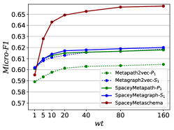
(a) walk-times $w$.

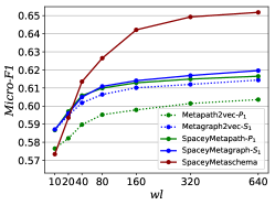
(b) walk-length $l$.

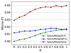
(c) personalized-probability $\alpha$.

Figure 4. Parameter sensitivity for author node classification on the ACM dataset.

4.5. Parameter Sensitivity

In this section, we illustrate the parameters sensitivity by the Micro-F1 scores of author node classification experiments on the ACM dataset. For each experiment, we vary one parameter and fix the others as the default values (as shown in Sec. 4.2).

From Figure 4(a) and Figure 4(b), we can see that walk-times $w$ and walk-length $l$ are positive to performance for all random walk based algorithms, and the positivity gradually weakens with the parameter increasing. From Figure 4(c), we can see that the performance increases with the personalized probability $\alpha$ increasing, and the tend will be weakened when $\alpha$ reaches around 0.7. Specially, from Figure 4, we can clearly observe that the proposed SpaceyMetapath/SpaceyMetagraph outperforms Metapath2vec/Metagraph2vec given a relatively small $w$ or $l$. For example, given meta-path $\mathcal{P}_{1}$ as the input, we can find that the performance of the proposed SpaceyMetapath with $l\!=\!40$ is equivalent to the performance of Metapath2vec with $l\!=\!640$, giving us around 16x speedup. Further, we randomly trace 1000 walk sequences of meta-path $\mathcal{P}_{1}$ guided spacey random walk and normal Marovian random walk respectively, and gradually compute the JS (Jensen–Shannon) divergence (Fuglede and Topsoe, 2004) of the node distributions between steps. The average variation is shown in Figure 5. Compared with Metapath2vec, we can evidently observe that the distribution divergence for SpaceyMetapath quickly descends to a small level with a small walk-length. Overall, above comparision analysis indicates that the proposed spacey random walk frameworks are able to reach high performance under a cost-effective parameter choice (the smaller, the more efficient).

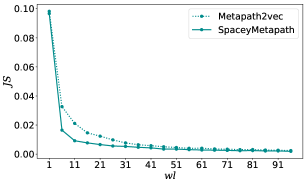
Figure 5. Variation of node distribution during meta-path “APVPA” guided random walks on the ACM dataset.

4.6. Complexity and Scalability Analysis

In this section, we demonstrate the scalability of the proposed frameworks by measuring both the walk time to generate heterogeneous neighborhood and the training time to learn node embeddings. We first follow the meta-schema of DBLP network to simulate a series of random graph datasets with the average degree of 10. The specific network sizes are [1k; 10k; 100k; 1000k; 10000k]. Then, we independently run experiments on these synthetic HINs in a computing server with $56$ core Intel(R) Xeon(R) CPU E5-2680 v4 @ 2.40GHz. The time consumption is shown in Figure 6, which shows that our methods all have a linear time complexity with respect to the number of nodes and can be easily applied to very large-scale networks. In fact, for the random walk phase in an HIN ${\mathcal{G}}=({\mathcal{V}},{\mathcal{E}};\mathcal{A},\mathcal{R})$ with walk-times $t$ and walk-length $l$, the spacey walk for each step takes $O(|\mathcal{A}|)$ time, and the total walk complexity is $O(wl|\mathcal{A}||\mathcal{V}|)$, which is linear to the number of nodes. For the training phase, we use a Skipgram model to train the embeddings of different types of nodes, which also has a linear complexity and can be parallelized by using the same mechanism as word2vec (Grover and Leskovec, 2016). Overall, the proposed algorithms are quite efficient and scalable for large-scale heterogeneous networks.

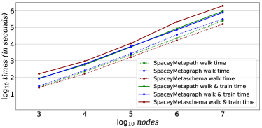
Figure 6. The walk and train time of the proposed models over different network sizes.

5. Related Work

In the past decade, to marry the advantages of HIN and network embedding, embedding learning in an HIN has received increasing attention and many heterogeneous embedding algorithms have been proposed (Bordes et al., 2013; Tang et al., 2015a; Chang et al., 2015; Dong et al., 2017; Zhang et al., 2018a; Kralj et al., 2018; Qiu et al., 2018; Sun et al., 2018; Shi et al., 2018b).

In general, there have been multiple ways to represent multi-typed nodes in an HIN. A straightforward method is to directly perform matrix/tensor factorization (Maruhashi et al., 2012; Papalexakis et al., 2017; Qiu et al., 2018) to extract vector representations of nodes. For example, Collective matrix factorization of multi-type relational data (Singh and Gordon, 2008; Nickel et al., 2012; Bouchard et al., 2013) treats each binary relation as a matrix, and performs joint matrix factorization over different relations. However, such a way is usually costly for computation and memory. More recently, researchers apply stochastic optimization to optimize simple or deep models to predict the binary relations between two types of entities with large-scale knowledge graphs (Nickel et al., 2016). Representative approach include TransE (Bordes et al., 2013) where one entity in a type is translated by a relation vector to another entity in another type given the co-occurrence of a binary relations between them and PTE (Tang et al., 2015a) which decomposes an HIN to a set of bipartite networks by edge types, and learns node vectors by capturing 1-hop neighborhood of the resulting bipartite networks. All of these methods, although sometimes called higher-order factorization or embedding, are still dealing with the co-occurrence of binary relations among entities (Nickel et al., 2016). More recently, inspired by the DeepWalk model for homogeneous networks (Perozzi et al., 2014), meta-paths or meta-graphs guided random walk based entity embedding models have also been well developed (Shang et al., 2016; Dong et al., 2017; Fu et al., 2017; Shi et al., 2018a; Zhang et al., 2018b) using the Skipgram techniques introduced by word2vec (Mikolov et al., 2013b) for very large graphs. However, as discussed in Section 1, these algorithms have few attention on the higher-order Markov chain nature of meta-path guided random walk. Following random walk based embedding algorithms, we focus on the higher-order Markov chains and design a new meta-path/meta-graph guided random walk strategy, and further develop several general scalable HIN embedding models.

6. Conclusions

In this paper, we propose a heterogeneous personalized spacey random walk strategy to efficiently generate heterogeneous neighborhood, which is based on a solid mathematical foundation. We further develop a scalable HIN embedding algorithms SpaceyMetapath to efficiently and effectively produce node embeddings in an HIN guided by an arbitrary meta-path. We also develop two scalable HIN embedding algorithms by extending the SpaceyMetapath from a meta-path to a meta-graph or a meta-schema. Experimental results show that our methods are able to achieve better performance with smaller walk-times and walk-length.

7. Acknowledgments

This work is supported by the China NSFC program (No.61872022, 61421003) , SKLSDE-2018ZX16, and the Early Career Scheme (ECS, No.26206717) from Research Grants Council in Hong Kong. For any correspondence, please refer to Jianxin Li.

References

- (1)
- Benson et al. (2017) Austin R. Benson, David F. Gleich, and Lek-Heng Lim. 2017. The Spacey Random Walk: A Stochastic Process for Higher-Order Data. SIAM Rev. 59, 2 (2017), 321–345.
- Bordes et al. (2013) Antoine Bordes, Nicolas Usunier, Alberto Garcia-Duran, Jason Weston, and Oksana Yakhnenko. 2013. Translating Embeddings for Modeling Multi-relational Data. In NIPS. 2787–2795.
- Bouchard et al. (2013) Guillaume Bouchard, Dawei Yin, and Shengbo Guo. 2013. Convex Collective Matrix Factorization. In AISTATS. 144–152.
- Cai et al. (2018) Hongyun Cai, Vincent W Zheng, and Kevin Chen-Chuan Chang. 2018. A comprehensive survey of graph embedding: Problems, techniques, and applications. TKDE 30, 9 (2018), 1616–1637.
- Chang et al. (2015) Shiyu Chang, Wei Han, Jiliang Tang, Guo-Jun Qi, Charu C Aggarwal, and Thomas S Huang. 2015. Heterogeneous network embedding via deep architectures. In KDD. ACM, 119–128.
- Dong et al. (2017) Yuxiao Dong, Nitesh V. Chawla, and Ananthram Swami. 2017. metapath2vec: Scalable Representation Learning for Heterogeneous Networks. In KDD. 135–144.
- Fang et al. (2016) Yuan Fang, Wenqing Lin, Vincent Wenchen Zheng, Min Wu, Kevin Chen-Chuan Chang, and Xiaoli Li. 2016. Semantic proximity search on graphs with metagraph-based learning. In ICDE. 277–288.
- Fu et al. (2017) Tao-Yang Fu, Wang-Chien Lee, and Zhen Lei. 2017. HIN2Vec: Explore Meta-paths in Heterogeneous Information Networks for Representation Learning. In CIKM. 1797–1806.
- Fuglede and Topsoe (2004) Bent Fuglede and Flemming Topsoe. 2004. Jensen-Shannon divergence and Hilbert space embedding. In Information Theory, 2004. ISIT 2004. Proceedings. International Symposium on. IEEE, 31.
- Grover and Leskovec (2016) Aditya Grover and Jure Leskovec. 2016. node2vec: Scalable Feature Learning for Networks. In KDD. 855–864.
- Hu et al. (2018) Binbin Hu, Chuan Shi, Wayne Xin Zhao, and Philip S. Yu. 2018. Leveraging Meta-path based Context for Top- N Recommendation with A Neural Co-Attention Model. In KDD. ACM, 1531–1540.
- Huang et al. (2016) Zhipeng Huang, Yudian Zheng, Reynold Cheng, Yizhou Sun, Nikos Mamoulis, and Xiang Li. 2016. Meta Structure: Computing Relevance in Large Heterogeneous Information Networks. In SIGKDD. 1595–1604.
- Kralj et al. (2018) Jan Kralj, Marko Robnik-Šikonja, and Nada Lavrač. 2018. HINMINE: heterogeneous information network mining with information retrieval heuristics. Journal of Intelligent Information Systems 50, 1 (2018), 29–61.
- Lao and Cohen (2010) Ni Lao and William W. Cohen. 2010. Relational retrieval using a combination of path-constrained random walks. Machine Learning 81, 1 (2010), 53–67.
- Li and Ng (2014) Wen Li and Michael K Ng. 2014. On the limiting probability distribution of a transition probability tensor. Linear and Multilinear Algebra 62, 3 (2014), 362–385.
- Maruhashi et al. (2012) Koji Maruhashi, Fan Guo, and Christos Faloutsos. 2012. MultiAspectForensics: mining large heterogeneous networks using tensor. Int. J. Web Eng. Technol. 7, 4 (2012), 302–322.
- Mikolov et al. (2013a) Tomas Mikolov, Kai Chen, Greg Corrado, and Jeffrey Dean. 2013a. Efficient estimation of word representations in vector space. arXiv preprint arXiv:1301.3781 (2013).
- Mikolov et al. (2013b) Tomas Mikolov, Ilya Sutskever, Kai Chen, Greg S Corrado, and Jeff Dean. 2013b. Distributed representations of words and phrases and their compositionality. In NIPS. 3111–3119.
- Nickel et al. (2016) Maximilian Nickel, Kevin Murphy, Volker Tresp, and Evgeniy Gabrilovich. 2016. A Review of Relational Machine Learning for Knowledge Graphs. Proc. IEEE 104, 1 (2016), 11–33.
- Nickel et al. (2012) Maximilian Nickel, Volker Tresp, and Hans-Peter Kriegel. 2012. Factorizing YAGO: scalable machine learning for linked data. In WWW. 271–280.
- Papalexakis et al. (2017) Evangelos E. Papalexakis, Christos Faloutsos, and Nicholas D. Sidiropoulos. 2017. Tensors for Data Mining and Data Fusion: Models, Applications, and Scalable Algorithms. ACM TIST 8, 2 (2017), 16:1–16:44.
- Perozzi et al. (2014) Bryan Perozzi, Rami Al-Rfou, and Steven Skiena. 2014. DeepWalk: online learning of social representations. In KDD. 701–710.
- Qiu et al. (2018) Jiezhong Qiu, Yuxiao Dong, Hao Ma, Jian Li, Kuansan Wang, and Jie Tang. 2018. Network embedding as matrix factorization: Unifying deepwalk, line, pte, and node2vec. In WSDM. ACM, 459–467.
- Ren et al. (2015a) Xiang Ren, Ahmed El-Kishky, Chi Wang, and Jiawei Han. 2015a. Automatic Entity Recognition and Typing from Massive Text Corpora: A Phrase and Network Mining Approach. In KDD. 2319–2320.
- Ren et al. (2015b) Xiang Ren, Ahmed El-Kishky, Chi Wang, Fangbo Tao, Clare R. Voss, and Jiawei Han. 2015b. ClusType: Effective Entity Recognition and Typing by Relation Phrase-Based Clustering. In SIGKDD. 995–1004.
- Shang et al. (2016) Jingbo Shang, Meng Qu, Jialu Liu, Lance M Kaplan, Jiawei Han, and Jian Peng. 2016. Meta-path guided embedding for similarity search in large-scale heterogeneous information networks. arXiv preprint arXiv:1610.09769 (2016).
- Shi et al. (2018a) Chuan Shi, Binbin Hu, Xin Zhao, and Philip Yu. 2018a. Heterogeneous Information Network Embedding for Recommendation. IEEE Transactions on Knowledge and Data Engineering (2018).
- Shi et al. (2014) Chuan Shi, Xiangnan Kong, Yue Huang, S Yu Philip, and Bin Wu. 2014. HeteSim: A General Framework for Relevance Measure in Heterogeneous Networks. IEEE Trans. Knowl. Data Eng. 26, 10 (2014), 2479–2492.
- Shi et al. (2017) Chuan Shi, Yitong Li, Jiawei Zhang, Yizhou Sun, and S Yu Philip. 2017. A survey of heterogeneous information network analysis. TKDE 29, 1 (2017), 17–37.
- Shi et al. (2015) Chuan Shi, Zhiqiang Zhang, Ping Luo, Philip S Yu, Yading Yue, and Bin Wu. 2015. Semantic path based personalized recommendation on weighted heterogeneous information networks. In Proceedings of the 24th ACM International on Conference on Information and Knowledge Management. ACM, 453–462.
- Shi et al. (2018b) Yu Shi, Qi Zhu, Fang Guo, Chao Zhang, and Jiawei Han. 2018b. Easing Embedding Learning by Comprehensive Transcription of Heterogeneous Information Networks. In KDD. ACM, 2190–2199.
- Singh and Gordon (2008) Ajit P. Singh and Geoffrey J. Gordon. 2008. Relational Learning via Collective Matrix Factorization. In KDD. 650–658.
- Sun et al. (2018) Lichao Sun, Lifang He, Zhipeng Huang, Bokai Cao, Congying Xia, Xiaokai Wei, and S Yu Philip. 2018. Joint embedding of meta-path and meta-graph for heterogeneous information networks. In ICBK. IEEE, 131–138.
- Sun and Han (2012) Yizhou Sun and Jiawei Han. 2012. Mining heterogeneous information networks: principles and methodologies. Synthesis Lectures on Data Mining and Knowledge Discovery 3, 2 (2012), 1–159.
- Sun et al. (2011) Yizhou Sun, Jiawei Han, Xifeng Yan, Philip S. Yu, and Tianyi Wu. 2011. PathSim: Meta Path-Based Top-K Similarity Search in Heterogeneous Information Networks. PVLDB (2011), 992–1003.
- Sun et al. (2012) Yizhou Sun, Brandon Norick, Jiawei Han, Xifeng Yan, Philip S. Yu, and Xiao Yu. 2012. Integrating meta-path selection with user-guided object clustering in heterogeneous information networks. In KDD. 1348–1356.
- Tang et al. (2015a) Jian Tang, Meng Qu, and Qiaozhu Mei. 2015a. PTE: Predictive Text Embedding through Large-scale Heterogeneous Text Networks. (2015), 1165–1174.
- Tang et al. (2015b) Jian Tang, Meng Qu, Mingzhe Wang, Ming Zhang, Jun Yan, and Qiaozhu Mei. 2015b. LINE: Large-scale Information Network Embedding. In WWW. 1067–1077.
- Yu et al. (2014) Xiao Yu, Xiang Ren, Yizhou Sun, Quanquan Gu, Bradley Sturt, Urvashi Khandelwal, Brandon Norick, and Jiawei Han. 2014. Personalized entity recommendation: a heterogeneous information network approach. In WSDM. 283–292.
- Zhang et al. (2018a) Chuxu Zhang, Ananthram Swami, and Nitesh V Chawla. 2018a. CARL: Content-Aware Representation Learning for Heterogeneous Networks. arXiv preprint arXiv:1805.04983 (2018).
- Zhang et al. (2018b) Daokun Zhang, Jie Yin, Xingquan Zhu, and Chengqi Zhang. 2018b. MetaGraph2Vec: Complex Semantic Path Augmented Heterogeneous Network Embedding. In PAKDD. Springer, 196–208.
- Zhao et al. (2017) Huan Zhao, Quanming Yao, Jianda Li, Yangqiu Song, and Dik Lun Lee. 2017. Meta-Graph Based Recommendation Fusion over Heterogeneous Information Networks. In KDD. ACM, 635–644.
- Zheng et al. (2017) Jing Zheng, Jian Liu, Chuan Shi, Fuzhen Zhuang, Jingzhi Li, and Bin Wu. 2017. Recommendation in heterogeneous information network via dual similarity regularization. International Journal of Data Science and Analytics 3, 1 (2017), 35–48.