Structure constants of heavy operators

in ABJM/ABJ Theory

Gaoli Chen^b,, Robert de Mello Koch^a,b,, Minkyoo Kim^b,

and Hendrik J.R. Van Zyl^b,

^a School of Physics and Telecommunication Engineering,

South China Normal University, Guangzhou 510006, China

^b National Institute for Theoretical Physics,

School of Physics and Mandelstam Institute for Theoretical Physics,

University of the Witwatersrand, Wits, 2050,

South Africa

ABSTRACT

Efficient and powerful approaches to the computation of correlation functions involving determinant, sub-determinant and permanent operators, as well as traces, have recently been developed in the setting of ${\cal N}=4$ super Yang-Mills theory. In this article we show that they can be extended to ABJM and ABJ theory. After making use of a novel identity which follows from character orthogonality, an integral representation of certain projection operators used to define Schur polynomials is given. This integral representation provides an effective description of the correlation functions of interest. The resulting effective descriptions have ${1\over N}$ as the loop counting parameter, strongly suggesting their relevance for holography.

1 Introduction

The discovery of integrability in the planar limit of ${\cal N}=4$ super Yang-Mills theory[1] has provided important lessons into gauge/gravity duality[2, 3, 4]. The planar spectrum can be computed exactly to all order in $\lambda$ and it can be matched to string theory - a remarkable achievement[5].

By restricting to the planar limit, we are necessarily restricting attention to operators with a dimension that obeys $\Delta^{2}\ll N$[6]. This is a tiny part of the theory and to properly understand gauge/gravity duality we will presumably have to consider operators with a dimension of order $N$ or even order $N^{2}$. These have a sensible physical interpretation as branes[6, 7, 8, 9] and new geometries[10] respectively. The study of these large dimension operators is challenging. In general, we do not expect any integrability. Further, the usual description of the large $N$ expansion as a genus expansion for sums of ribbon graphs is not a valid description and all the known lore of large $N$ must be revisited.

In this study we consider correlation functions involving operators with a dimension of order $N_{1}$ in a supersymmetric ${\cal N}=6$ Chern-Simons-matter theory with gauge group $U(N_{1})_{k}\times U(N_{2})_{-k}$, where $k$ denotes the Chern-Simons level and we assume that $N_{1}\sim N_{2}$. Our notation is $N_{1}\geq N_{2}$. There is an AdS₄/CFT₃ duality which relates this Chern-Simons matter theory to type IIA string theory on AdS${}_{4}\times$CP³ with non-zero background fluxes. There are $N_{2}$ units of RR four-form flux through AdS₄, $k$ units of RR two-form flux through a CP${}^{1}\subset$CP³ and NS B-field $B_{2}$ with non-trivial holonomy

$${1\over 2\pi}\int_{{\rm CP}^{1}\subset{\rm CP}^{3}}B_{2}={N_{1}-N_{2}\over k}$$ (1.1)

For $N_{1}=N_{2}$ the Chern-Simons-matter theory is known as ABJM theory[11]. The general case ($N_{1}\neq N_{2}$) is denoted ABJ theory[12]. The fields can be rescaled by powers of ${1\over k}$ so that all interaction vertices are suppressed by powers of ${1\over k}$. Thus, the level $k$ plays the role of the coupling constant and large $k$ is weak coupling. The planar limit is given by

$$k,N\to\infty\qquad\lambda\equiv{N\over k}={\rm fixed}$$ (1.2)

Integrability makes an appearance in this limit[13]. The theory has two gauge fields, one in the adjoint of $U(N_{1})$ and one in the adjoint of $U(N_{2})$, four complex scalars and four Majorana fermions. The scalars and fermions are both in the $N_{1}\times\bar{N}_{2}$ or $\bar{N}_{1}\times N_{2}$ of $U(N_{1})\times U(N_{2})$. We study determinant, sub determinant and permanent operators constructed using only the four complex scalars.

Our goal is to generalize the recently developed techniques of [14, 15] in the AdS₅/CFT₄ setting to the AdS₄/CFT₃ setting. Denote the four complex scalar fields by $A_{i}$ and $B_{i}$, $i=1,2$. Let $a=1,...,N_{1}$ be a gauge group index for $U(N_{1})$ and let $\alpha=1,...,N_{2}$ be a gauge group index for $U(N_{2})$. Indicating gauge indices we have $(A_{i})^{a}_{\alpha}$ and $(B_{i})^{a}_{\alpha}$. In this study we work entirely in the free theory. The free field theory action is given by

$$S=k\int d^{3}x\left(\partial_{\mu}(A_{i})^{a}_{\alpha}\partial^{\mu}(A_{i}^{\dagger})_{a}^{\alpha}+\partial_{\mu}(B_{i})^{a}_{\alpha}\partial^{\mu}(B_{i}^{\dagger})_{a}^{\alpha}\right)$$ (1.3)

Notice that the composite field $(\phi_{ij})^{a}_{b}=(A_{i})^{a}_{\alpha}(B_{j}^{\dagger})^{\alpha}_{b}$ transforms in the adjoint of $U(N_{1})$. The heavy operators that we are interested in can be described as Schur polynomials in the matrix $Z=\phi_{11}$ or $Z^{\dagger}$ [16, 17, 18]. As in ${\cal N}=4$ super Yang-Mills theory, the Schur polynomials provide a complete basis for local operators constructed from $Z$ and they diagonalize the free field theory two point function[16, 17, 18]

$$\langle\chi_{R}(x_{1})\chi_{S}(x_{2})^{\dagger}\rangle=\delta_{RS}f_{R}(N_{1})f_{R}(N_{2})\left({1\over 4\pi k|x_{1}-x_{2}|}\right)^{n}$$ (1.4)

where $R$ is a Young diagram with $n$ boxes, i.e. $R\vdash n$. $f_{R}(N)$ is a product of factors, one for each box in $R$, with the factor for a box in row $i$ and column $j$ given by $N-i+j$. The stringy exclusion principle is implemented by requiring that $R$ has no more than $N_{2}$ rows. We will also consider restricted Schur polynomials in the ABJM theory, constructed using $\phi_{11}$ and $\phi_{12}$[19]. Operators constructed using $n_{11}$ $\phi_{11}$ fields and $n_{12}$ $\phi_{12}$ fields are labeled by three Young diagrams, $r\vdash n_{11}$, $s\vdash n_{12}$ and $R\vdash n$ with $n=n_{11}+n_{12}$. The pair $(r,s)$ label an irreducible representation that can be obtained from the irreducible representation $R$ of $S_{n}$ after restricting to the $S_{n_{11}}\times S_{n_{12}}$ subgroup. The representation $(r,s)$ may appear more than once after restricting and consequently we need a multiplicity label to distinguish the different copies. The relevant two point function is given by

$$\langle\chi_{R,(r,s)\alpha\beta}(x_{1})\chi_{T,(t,u)\gamma\tau}^{\dagger}(x_{2})\rangle=\delta_{RS}\delta_{rt}\delta_{su}\delta_{\alpha\gamma}\delta_{\beta\tau}{{\rm hooks}_{R}f_{R}(N_{1})^{2}\over{\rm hooks}_{r}{\rm hooks}_{s}}\left({1\over 4\pi k|x_{1}-x_{2}|}\right)^{n}$$ (1.5)

where ${\rm hooks}_{t}$ stands for the product of hook lengths in Young diagram $t$ and the indices $\alpha,\beta,\gamma,\tau$ are multiplicity labels. For a careful and elegant treatment of the effects of the stringy exclusion principle see [20].

The string theory duals to these heavy operators are giant gravitons branes in IIA string theory. Operators labeled by Young diagrams with $O(1)$ long rows (of length $\sim N_{1}\sim N_{2}$) correspond to dual giant gravitons, given by $D2$ branes wrapping an S${}^{2}\subset$AdS₄[21, 22, 23, 24]. Operators labeled by Young diagrams with $O(1)$ long columns (of length $\sim N_{1}\sim N_{2}$) correspond to giant gravitons, given by $D4$ branes wrapping a four manifold in CP³[25, 26, 27].

The paper is organized as follows: In Section 2 we discuss correlation functions involving determinants. We start with a discussion of maximal giant gravitons in the ABJM theory and then generalize the discussion to general giant gravitons in both ABJM and ABJ theory. In Section 3 the discussion is generalized to correlation functions of permanents, relevant for dual giant gravitons. This is followed in Section 4 with a discussion of restricted Schur polynomials which are dual to giant gravitons carrying more than one angular momentum. Following [14, 15] we explain in Section 5, that the effective theories that we obtain can be understood in terms of a graph duality proposed by [28]. In an attempt to gain further insight into the $\rho$ theory, we consider a saddle point evaluation of the $\rho$ integral in Section 6, which allows us to obtain the correct leading contribution to the correlators in the large $N$ limit. An interesting feature of this analysis, for the ABJ theory, is the existence of a pair of saddle points related by parity. Finally in section 7 we discuss our results and draw some conclusions.

2 Correlators involving Determinants and Subdeterminants

The maximal giant gravitons in the Anti-de Sitter spacetime are dual to determinant operators in the CFT so that we will refer to the determinant operators as maximal giant gravitons. We are interested in computing the correlation function of $Q$ maximal giant gravitons, located at positions $x_{A}$, for $A=1,2,...,Q$. The giant at $x_{A}$ is given by the Schur polynomial $\chi_{(1^{N_{1}})}(x_{A})$. The Schur polynomial located at $x_{A}$ is constructed using the field $({\cal Z}_{A})^{a}_{b}(x_{A})$, which is a linear combination of products of pairs of the complex scalar fields, each transforming in the adjoint of $U(N_{1})$. The only assumption we make is that

$$\left\langle({\cal Z}_{K})^{a}_{b}(x_{K})({\cal Z}_{K})^{c}_{d}(x_{K})\right\rangle=0$$ (2.1)

which ensures that our composite operator is free of UV divergences. For simplicity, to start, consider the ABJM theory. Introduce two sets of fermionic vectors, $\chi^{a},\bar{\chi}_{a}$ and $\psi^{\alpha},\bar{\psi}_{\alpha}$ and note that

$$\int[d^{N_{1}}\bar{\chi}d^{N_{1}}\chi][d^{N_{1}}\bar{\psi}d^{N_{1}}\psi]\bar{\psi}_{\beta_{1}}\psi^{\alpha_{1}}\cdots\bar{\psi}_{\beta_{N_{1}}}\psi^{\alpha_{N_{1}}}\bar{\chi}_{b_{1}}\chi^{a_{1}}\cdots\bar{\chi}_{b_{N_{1}}}\chi^{a_{N_{1}}}$$ (2.2)

$$=\sum_{\sigma,\rho\in S_{N_{1}}}\chi_{(1^{N_{1}})}(\sigma)\chi_{(1^{N_{1}})}(\rho)\sigma^{\bf\alpha}_{\bf\beta}\rho^{\bf a}_{\bf b}$$ (2.3)

where

$$\sigma^{\bf\alpha}_{\bf\beta}=\delta^{\alpha_{1}}_{\beta_{\sigma(1)}}\cdots\delta^{\alpha_{N_{1}}}_{\beta_{\sigma(N_{1})}}\qquad\qquad\rho^{\bf a}_{\bf b}=\delta^{a_{1}}_{b_{\rho(1)}}\cdots\delta^{a_{N_{1}}}_{b_{\rho(N_{2})}}$$ (2.4)

The label $(1^{N_{1}})$ stands for a Young diagram with a single column of $N_{1}$ boxes. We will now argue that the right hand side of the above identity is the projection operator that appears in the definition of maximal giant gravitons in the ABJM theory. Using the Fundamental Orthogonality Relation for matrix elements of irreducible representations[29], it is simple to prove the identity

$$\sum_{\sigma,\rho}\chi_{R}(\sigma)\chi_{S}(\rho){\rm Tr}(\sigma A^{\otimes N_{1}}\rho B^{\dagger\,\otimes N_{1}})={\delta_{RS}N_{1}!\over d_{R}}\sum_{\psi\in S_{N_{1}}}\chi_{R}(\psi)(AB^{\dagger})^{\alpha_{1}}_{\alpha_{\psi(1)}}\cdots(AB^{\dagger})^{\alpha_{N_{1}}}_{\alpha_{\psi(N_{1})}}$$ (2.5)

As usual there is a Schur-Weyl duality that (in the most general case of ABJ theory) organizes both the representations of $U(N_{1})$ and $U(N_{2})$. For the example we are considering here the centralizer is $S_{N_{1}}$. In general we could have $n\neq N_{1}$ fields and the same identity would hold, after replacing $N_{1}\to n$. The centralizer in this more general case is $S_{n}$ - which swaps $A$s and $B^{\dagger}$s. Notice that it is the same $S_{n}$ that is the centralizer for both $U(N_{1})$ and $U(N_{2})$ and this is why we get the $\delta_{RS}$ above. The reader should also note that it is only the symmetric group that played a role in the derivation of the above formula, so that it is also applicable in the ABJ theory where $N_{1}\neq N_{2}$.

Using the identity above we will be able to write an integral representation for the maximal giant graviton correlation functions. To carry out a general discussion introduce a set of vectors $\cal{Y}_{K}$ which we dot with $\phi^{I}=(A_{1},A_{2},B_{1},B_{2})$ and a set of vectors $\bar{\cal{Y}}_{K}$ which we dot with $\phi^{I{\dagger}}=(A_{1}^{\dagger},A_{2}^{\dagger},B_{1}^{\dagger},B_{2}^{\dagger})$. For now keep these vectors general up to the $Q$ conditions $\bar{\cal{Y}}_{K}\cdot{\cal{Y}}_{K}=0$, which ensure contractions of fields inside the same giant vanish, consistent with (2.1). The correlation function of $Q$ giant gravitons and a single trace operator ${\cal O}$ can be written as

$$\left\langle\chi_{(1^{N_{1}})}(x_{1})\chi_{(1^{N_{1}})}(x_{2})\cdots\chi_{(1^{N_{1}})}(x_{Q})\,{\cal O}\right\rangle=\int[d\phi^{I}d\phi^{I\,\dagger}]\int\prod_{K=1}^{Q}[d^{N_{1}}\bar{\chi}_{K}d^{N_{1}}\chi_{K}][d^{N_{1}}\bar{\psi}_{K}d^{N_{1}}\psi_{K}]$$ (2.6)

$$e^{-k\int d^{3}x\left(\partial_{\mu}\phi^{I}\cdot\partial^{\mu}(\phi^{I})^{\dagger}+\frac{1}{k}\sum_{K=1}^{Q}\delta(x-x_{K})(\bar{\chi}_{aK}({\cal{Y}_{K}\cdot\phi^{I}})^{a}_{\alpha}\psi_{K}^{\alpha}-\bar{\psi}_{\alpha K}(\bar{\cal{Y}}_{K}\cdot(\phi^{I})^{\dagger})^{\alpha}_{a}\chi_{K}^{a})\right)}{\cal O}(\phi^{I},\phi^{I\dagger})$$ (2.7)

The first step is to perform the Gaussian integral over the adjoint scalars which leads to

$$\left\langle\chi_{(1^{N_{1}})}(x_{1})\chi_{(1^{N_{1}})}(x_{2})\cdots\chi_{(1^{N_{1}})}(x_{Q})\,{\cal O}\right\rangle=\int\prod_{K=1}^{Q}\left[d^{N_{1}}\bar{\chi}_{K}d^{N_{1}}\chi_{K}\right]\left[d^{N_{1}}\bar{\psi}_{K}d^{N_{1}}\psi_{K}\right]$$ (2.9)

$$\qquad\qquad e^{\frac{1}{4k\pi}\sum_{K\neq J=1}^{Q}\frac{{\bar{\cal{Y}}}_{K}\cdot{\cal{Y}}_{J}}{x_{JK}}\left(\bar{\psi}_{\alpha K}\psi_{J}^{\alpha}\bar{\chi}_{aJ}\chi_{K}^{a}\right)}{\cal O}(S,S^{\dagger})$$ (2.10)

where

$$(S^{I})^{a}_{\alpha}={1\over k}\sum_{K=1}^{Q}\frac{1}{4\pi|x-x_{K}|}\left({\bar{\cal{Y}}}^{I}_{K}\bar{\psi}_{\alpha K}\chi_{K}^{a}\right)\qquad(S^{I{\dagger}})^{\alpha}_{a}=-{1\over k}\sum_{K=1}^{Q}\frac{1}{4\pi|x-x_{K}|}\left({\cal{Y}}^{I}_{K}\bar{\chi}_{aK}\psi_{K}^{\alpha}\right)$$ (2.11)

We now perform a Hubbard-Stratonovich transformation, introducing a complex matrix $\rho_{JK}$ and replacing the quartic dependence on the fermion vectors with a quadratic dependence. It is then possible to integrate over the fermionic vectors to obtain

$$\left\langle\chi_{(1^{N_{1}})}(x_{1})\chi_{(1^{N_{1}})}(x_{2})\cdots\chi_{(1^{N_{1}})}(x_{Q})\,{\cal O}\right\rangle$$ (2.12)

$$\qquad\qquad=\int[d\rho\,d\rho^{\dagger}]e^{-4\pi{N_{1}\over\lambda}{\rm Tr}(\rho^{\dagger}\rho)+N_{1}{\rm Tr}\log\left(M_{1}\right)+N_{1}{\rm Tr}\log\left(M_{2}\right)}\langle{\cal O}(S,S^{\dagger})\rangle_{\chi,\psi}$$ (2.13)

where

$$(M_{1})_{JK}=-\sqrt{\frac{\bar{\cal Y}_{K}\cdot{\cal Y}_{J}}{|x_{KJ}|}}\rho_{KJ}\qquad\qquad(M_{2})_{KJ}=-\sqrt{\frac{\bar{\cal Y}_{K}\cdot{\cal Y}_{J}}{|x_{KJ}|}}\rho^{\dagger}_{JK}$$ (2.14)

and the measure is normalized so that

$$\int[d\rho\,d\rho^{\dagger}]e^{-4\pi{N_{1}\over\lambda}{\rm Tr}\left(\rho\rho^{\dagger}\right)}=1$$ (2.15)

The integration over the fermionic vectors contracts the fermions appearing in $S$ and $S^{\dagger}$. The result after the contractions are performed is denoted by $\langle{\cal O}(S,S^{\dagger})\rangle_{\chi,\psi}$ in (2.13). These contractions are carried out by applying Wick’s theorem as usual with the following contractions

$$\langle\bar{\chi}_{Ka}\chi^{b}_{J}\rangle=\delta^{b}_{a}(M_{1}^{-1})_{KJ}\qquad\langle\bar{\psi}_{Ka}\psi^{b}_{J}\rangle=\delta^{b}_{a}(M_{2}^{-1})_{KJ}$$ (2.16)

Notice that a saddle point evaluation of (2.13) naturally generates the ${1\over N_{1}}$ expansion.

As a test of (2.13), we will consider the two-point function $\langle\chi_{(1^{N_{1}})}(AB^{\dagger})\chi_{(1^{N_{1}})}(A^{\dagger}B)\rangle$ of two giant gravitons in free ABJM theory. In this case we have

$$\rho=\left(\begin{array}[]{cc}0&z_{1}\\ z_{2}&0\end{array}\right)\qquad M_{1}=-\frac{1}{\sqrt{|x_{12}|}}\left(\begin{array}[]{cc}0&z_{2}\\ z_{1}&0\end{array}\right)\qquad M_{2}=-\frac{1}{\sqrt{|x_{12}|}}\left(\begin{array}[]{cc}0&z_{1}^{*}\\ z_{2}^{*}&0\end{array}\right)$$ (2.17)

Using polar coordinates for the complex numbers $z_{1},z_{2}$ we find

$$\langle\chi_{(1^{N_{1}})}(AB^{\dagger})(x_{1})\,\,\chi_{(1^{N_{1}})}(A^{\dagger}B)(x_{2})\rangle = \frac{64N_{1}^{2}\pi^{2}}{\lambda^{2}}\frac{1}{|x_{12}|^{2N_{1}}}\int dr_{1}\int dr_{2}e^{-\frac{4\pi N_{1}}{\lambda}(r_{1}^{2}+r_{2}^{2})}r_{1}^{2N_{1}+1}r_{2}^{2N_{1}+1}$$ (2.18)

$$= (N_{1}!)^{2}\left(\frac{1}{4\pi k|x_{12}|}\right)^{2N_{1}}$$ (2.19)

which agrees with (1.4). Now consider the same computation in the free ABJ theory and recall that $N_{1}\geq N_{2}$. The only significant difference between the ABJM and ABJ theories is in the initial integral expression for the correlator. The relevant integral representation for the ABJ theory is

$$\left\langle\chi_{(1^{N_{2}})}(x_{1})\chi_{(1^{N_{2}})}(x_{2})\cdots\chi_{(1^{N_{2}})}(x_{Q})\,{\cal O}\right\rangle=\int[d\phi^{I}d\phi^{I\dagger}]\int\prod_{K=1}^{Q}[d^{N_{1}}\bar{\chi}_{K}d^{N_{1}}\chi_{K}][d^{N_{2}}\bar{\psi}_{K}d^{N_{2}}\psi_{K}]$$ (2.20)

$$e^{-k\int d^{3}x\left(\partial_{\mu}\phi^{I}\cdot\partial^{\mu}(\phi^{I})^{\dagger}+\frac{1}{k}\sum_{K=1}^{Q}\delta(x-x_{K})(\bar{\chi}_{aK}({\cal{Y}_{K}\cdot\phi^{I}})^{a}_{\alpha}\psi_{K}^{\alpha}-\bar{\psi}_{\alpha K}(\bar{\cal{Y}}_{K}\cdot(\phi^{I})^{\dagger})^{\alpha}_{a}\chi_{K}^{a}+\bar{\chi}_{aK}\chi^{a}_{K})\right)}{\cal O}(\phi^{I},\phi^{I\dagger})$$ (2.21)

The important difference in the ABJ expression above and the ABJM expression in (2.7) is that there is an extra term $\bar{\chi}_{aK}\chi^{a}_{K}$ appearing in the effective action, needed to “soak up” the extra $\chi,\bar{\chi}$ integrations. It is a simple matter to repeat the analysis above with this new starting point.

The above results for determinants can be generalized to sub determinants. This corresponds to studying correlators of operators dual to giants gravitons that are not necessarily maximal. A useful identity is

$$\int[d^{N_{1}}\bar{\chi}d^{N_{1}}\chi][d^{N_{2}}\bar{\psi}d^{N_{2}}\psi]\bar{\chi}_{b_{1}}\chi^{a_{1}}\cdots\bar{\chi}_{b_{n}}\chi^{a_{n}}(\bar{\chi}\cdot\chi)^{N_{1}-n}\bar{\psi}_{\beta_{1}}\psi^{\alpha_{1}}\cdots\bar{\psi}_{\beta_{n}}\psi^{\alpha_{n}}(\bar{\psi}\cdot\psi)^{N_{2}-n}$$ (2.23)

$$=(-1)^{N_{1}-N_{2}}(N_{1}-n)!(N_{2}-n)!\sum_{\sigma,\rho\in S_{n}}\chi_{(1^{n})}(\sigma)\chi_{(1^{n})}(\rho)\sigma^{\bf\alpha}_{\bf\beta}\rho^{\bf a}_{\bf b}$$ (2.24)

where now

$$\sigma^{\bf\alpha}_{\bf\beta}=\delta^{\alpha_{1}}_{\beta_{\sigma(1)}}\cdots\delta^{\alpha_{n}}_{\beta_{\sigma(n)}}\qquad\rho^{\bf a}_{\bf b}=\delta^{a_{1}}_{b_{\rho(1)}}\cdots\delta^{a_{n}}_{b_{\rho(n)}}$$ (2.25)

The right hand side of the identity (2.24) is the projection operator needed to define sub determinant operators. Thus, the generating function for giant graviton correlators can be written as follows

$$\sum_{i_{1},i_{2},\cdots i_{Q}=1}^{N}t_{1}^{2i_{1}}\cdots t_{Q}^{2i_{Q}}\left\langle\chi_{(1^{i_{1}})}(x_{1})\cdots\chi_{(1^{i_{Q}})}(x_{Q})\,{\cal O}\right\rangle=\int[d\phi^{I}d\phi^{I\dagger}]\int\prod_{K=1}^{Q}[d^{N_{1}}\bar{\chi}_{K}d^{N_{1}}\chi_{K}][d^{N_{2}}\bar{\psi}_{K}d^{N_{2}}\psi_{K}]$$ (2.26)

$$e^{-k\int d^{3}x\,\left\{\partial_{\mu}\phi^{I}\partial^{\mu}\phi^{I\dagger}+{1\over k}\sum_{K=1}^{Q}\delta\left(x-x_{K}\right)\left[\bar{\chi}_{K}\cdot\chi_{K}+\bar{\psi}_{K}\cdot\psi_{K}+t_{K}\bar{\chi}_{K}\mathcal{Z}_{K}\psi_{K}-t_{K}\bar{\psi}_{K}\bar{\mathcal{Z}}_{K}\chi_{K}\right]\right\}}{\cal O}(\phi^{I},\phi^{I\dagger})$$ (2.27)

(2.28)

where we have suppressed the gauge indices and

$$\mathcal{Z}_{K}\equiv\sum_{I=1}^{4}\mathcal{Y}_{K}^{I}\phi^{I}\qquad\qquad\bar{\mathcal{Z}}_{K}=\sum_{I=1}^{4}\bar{\mathcal{Y}}_{K}^{I}\phi^{I\dagger}$$ (2.29)

After integrating over the $\phi^{I}$ fields, performing a Hubbard-Stratonovich transformation and then integrating over the fermionic vectors, we obtain

$$\sum_{i_{1},i_{2},\cdots i_{Q}=1}^{N}t_{1}^{2i_{1}}t_{2}^{2i_{2}}\cdots t_{Q}^{2i_{Q}}\left\langle\chi_{(1^{i_{1}})}(x_{1})\chi_{(1^{i_{2}})}(x_{2})\cdots\chi_{(1^{i_{Q}})}(x_{Q})\,{\cal O}\right\rangle=\int[d\rho d\rho^{\dagger}]\\ e^{-4\pi k{\rm Tr}\left(\rho\rho^{\dagger}\right)+N_{1}{\rm Tr}\ln\left[\delta_{JK}-\sqrt{\frac{t_{J}t_{K}\bar{\mathcal{Y}}_{K}\cdot\mathcal{Y}_{J}}{\left|x_{KJ}\right|}}\rho_{KJ}\right]+N_{2}{\rm Tr}\ln\left[\delta_{KJ}-\sqrt{\frac{t_{J}t_{K}\bar{\mathcal{Y}}_{K}\cdot\mathcal{Y}_{J}}{\left|x_{KJ}\right|}}\rho_{JK}^{\dagger}\right]}\left\langle\mathcal{O}^{I}\left(S^{I},S^{I{\dagger}}\right)\right\rangle_{\chi,\psi},$$ (2.30)

where

$$\left(S^{I}\right)_{\alpha}^{a}=\frac{1}{4\pi k}\sum_{K=1}^{Q}\frac{t_{K}\bar{\mathcal{Y}}_{K}^{I}\bar{\psi}_{K\alpha}\chi_{K}^{a}}{\left|x-x_{K}\right|},\quad\left(S^{I\dagger}\right)_{a}^{\alpha}=-\frac{1}{4\pi k}\sum_{K=1}^{Q}\frac{t_{K}\mathcal{Y}_{K}^{I}\bar{\chi}_{Ka}\psi_{K}^{\alpha}}{\left|x-x_{K}\right|}.$$ (2.31)

Here $\left\langle\mathcal{O}^{I}\left(S^{I},S^{I{\dagger}}\right)\right\rangle_{\chi,\psi}$ is again defined by Wick contracting all pairs of $\chi,{\bar{\chi}}$ and $\psi,{\bar{\psi}}$ fields according to Wick’s theorem, with the basic contraction given by

$$\left\langle\bar{\chi}_{aK}\chi_{L}^{b}\right\rangle=\delta_{a}^{b}\left(M_{1}^{-1}\right)_{KL}\qquad\qquad\left\langle\bar{\psi}_{\alpha K}\psi_{L}^{\beta}\right\rangle=\delta_{\alpha}^{\beta}\left(M_{2}^{-1}\right)_{KL}$$ (2.32)

with

$$\left(M_{1}\right)_{JK}=\delta_{JK}-\sqrt{\frac{t_{J}t_{K}\bar{\mathcal{Y}}_{K}\cdot\mathcal{Y}_{J}}{\left|x_{KJ}\right|}}\rho_{KJ}\qquad\left(M_{2}\right)_{KJ}=\delta_{KJ}-\sqrt{\frac{t_{J}t_{K}\bar{\mathcal{Y}}_{K}\cdot\mathcal{Y}_{J}}{\left|x_{KJ}\right|}}\rho_{JK}^{\dagger}$$ (2.33)

As a test of (2.30), we compute the two-point $\left\langle\chi_{(1^{J_{1}})}\left(AB^{\dagger}\right)\chi_{(1^{J_{2}})}\left(A^{\dagger}B\right)\right\rangle$. The exact result for this two point function is

$$\left\langle\chi_{(1^{J_{1}})}\left(AB^{\dagger}\right)(x_{1})\chi_{(1^{J_{2}})}\left(A^{\dagger}B\right)(x_{2})\right\rangle=\delta_{J_{1}J_{2}}\frac{N_{1}!}{\left(N_{1}-J_{1}\right)!}\frac{N_{2}!}{\left(N_{2}-J_{1}\right)!}\left({1\over 4\pi k|x_{1}-x_{2}|}\right)^{2J_{1}}$$ (2.34)

In this case, $\bar{\mathcal{Y}}_{1}\cdot\mathcal{Y}_{1}=\bar{\mathcal{Y}}_{2}\cdot\mathcal{Y}_{2}=0$ and $\bar{\mathcal{Y}}_{1}\cdot\mathcal{Y}_{2}=\bar{\mathcal{Y}}_{2}\cdot\mathcal{Y}_{1}=1$. Parameterize $\rho$ as

$$\rho=\begin{pmatrix}0&z_{1}\\ z_{2}&0\end{pmatrix}$$ (2.35)

The matrices $M_{1}$ and $M_{2}$ are then

$$M_{1}=\begin{pmatrix}1&-\sqrt{\frac{t_{1}t_{2}}{\left|x_{12}\right|}}z_{2}\\ -\sqrt{\frac{t_{1}t_{2}}{\left|x_{12}\right|}}z_{1}&1\end{pmatrix}\qquad\qquad M_{2}=\begin{pmatrix}1&-\sqrt{\frac{t_{1}t_{2}}{\left|x_{12}\right|}}z_{1}^{*}\\ -\sqrt{\frac{t_{1}t_{2}}{\left|x_{12}\right|}}z_{2}^{*}&1\end{pmatrix}$$ (2.36)

In this case, using (2.30), the computation boils down to computing the integral

$$\int[dz_{1}dz_{1}^{\dagger}dz_{2}dz_{2}^{\dagger}]\,e^{-4\pi k\left(|z_{1}|^{2}+|z_{2}|^{2}\right)}\det\left(M_{1}\right)^{N_{1}}\left(\det M_{2}\right)^{N_{2}}$$ (2.37)

Changing to polar coordinates $z_{i}=r_{i}e^{i\theta_{i}}$ and expanding the integrand as follows

$$\left(\det M_{1}\right)^{N_{1}}\left(\det M_{2}\right)^{N_{2}}=\sum_{l_{1},l_{2}}\binom{N_{1}}{l_{1}}\binom{N_{2}}{l_{2}}\left(-\frac{t_{1}t_{2}}{4\pi k\left|x_{1}-x_{2}\right|}\right)^{l_{1}+l_{2}}e^{i\left(l_{1}-l_{2}\right)\left(\theta_{1}+\theta_{2}\right)}$$ (2.38)

it is simple to find

$$\int[d\rho d\rho^{\dagger}]\,e^{-4\pi k{\rm Tr}\rho\rho^{\dagger}}\left(\det M_{1}\right)^{N_{1}}\left(\det M_{2}\right)^{N_{2}}=\sum_{l}\frac{N_{1}!}{\left(N_{1}-l\right)!}\frac{N_{2}!}{\left(N_{2}-l\right)!}\left(\frac{t_{1}t_{2}}{4\pi k\left|x_{1}-x_{2}\right|}\right)^{2l}$$ (2.39)

Extracting the coefficient of the $\left(t_{1}t_{2}\right)^{2J_{1}}$ term, we reproduce the exact result.

With the effective theory we can compute three point functions. Consider the correlation function

$$\langle\chi_{(1^{K+J})}(x_{1})\chi_{(1^{K})}(x_{2}){\cal O}_{J}(x_{3})\rangle$$ (2.40)

The Schur polynomial at $x_{1}$ is constructed using $Z^{\dagger}$, the Schur at $x_{2}$ is constructed using $Z$ and ${\cal O}_{J}$ is ${\rm Tr}(Z^{J})$. Here $K$ is order $N_{1}\sim N_{2}$, $J$ is order $1$ and we recall that $Z=A_{1}B^{\dagger}_{1}$. For generality, work in the ABJ model. Assume that $K+J$ is smaller than both $N_{1}$ and $N_{2}$. The spacetime dependence of this correlation function is rather simple

$$\langle\chi_{(1^{K+J})}(x_{1})\chi_{(1^{K})}(x_{2}){\cal O}_{J}(x_{3})\rangle={C_{K,J}\over(4\pi k|x_{1}-x_{2}|)^{2K}(4\pi k|x_{1}-x_{3}|)^{2J}}$$ (2.41)

where the coefficient $C_{K,J}$ can be computed in the zero dimensional version of the model, in which case it is given by

$$C_{K,J}=\langle\chi_{(1^{K+J})}(Z^{\dagger})\chi_{(1^{K})}(Z){\rm Tr}(Z^{J})\rangle$$ (2.42)

Using the identity

$${\rm Tr}(Z^{J})=\sum_{i=0}^{J-1}(-1)^{i}\chi_{(J-i,1^{i})}(Z)$$ (2.43)

we have

$$\chi_{(1^{K})}(Z){\rm Tr}(Z^{J})=(-1)^{J-1}\chi_{(1^{K+J})}(Z)+\cdots$$ (2.44)

where $\cdots$ above stands for terms with Schur polynomials that have more than a single column and hence don’t contribute to $C_{K,J}$. Consequently, we have

$$C_{K,J}=\langle\chi_{(1^{K+J})}(Z^{\dagger})\chi_{(1^{K})}(Z){\rm Tr}(Z^{J})\rangle=(-1)^{J-1}{N_{1}!\over(N_{1}-K-J)!}{N_{2}!\over(N_{2}-K-J)!}$$ (2.45)

so that

$$\langle\chi_{(1^{K+J})}(x_{1})\chi_{(1^{K})}(x_{2}){\cal O}_{J}(x_{3})\rangle=$$ (2.46)

$$\qquad\qquad(-1)^{J-1}{N_{1}!\over(N_{1}-K-J)!}{N_{2}!\over(N_{2}-K-J)!}{1\over(4\pi k|x_{1}-x_{2}|)^{2K}(4\pi k|x_{1}-x_{3}|)^{2J}}$$ (2.47)

Reproducing this result is a convincing check of the effective theory. We consider a more general case with

$$\mathcal{O}={\rm Tr}\left(\phi^{I_{1}}\phi^{\dagger\bar{I}_{1}}\phi^{I_{2}}\phi^{\dagger\bar{I}_{2}}\cdots\phi^{I_{J}}\phi^{\dagger\bar{I}_{J}}\right).$$ (2.49)

Recall that after integrating over the $\phi^{I}$ and $\phi^{I{\dagger}}$ fields, they become $S^{I}$’s and $S^{I{\dagger}}$’s. Consequently

$$\mathcal{O} = (-1)^{J}\left(\frac{1}{4\pi k}\right)^{2J}\sum_{K_{1},K_{2}\cdots K_{J}=1}^{Q}\sum_{\bar{K}_{1},\bar{K}_{2}\cdots\bar{K}_{J}=1}^{Q}t_{K_{1}}t_{\bar{K}_{1}}\cdots t_{K_{J}}t_{\bar{K}_{J}}\bar{\mathcal{Y}}_{K_{1}}^{I_{1}}\mathcal{Y}_{\bar{K}_{1}}^{\bar{I}_{1}}\cdots\bar{\mathcal{Y}}_{K_{J}}^{I_{J}}\mathcal{Y}_{\bar{K}_{J}}^{\bar{I}_{J}}$$ (2.50)

$$\times\frac{\bar{\psi}_{K_{1}\alpha_{J}}\chi_{K_{1}}^{a_{1}}\bar{\chi}_{\bar{K}_{1}a_{1}}\psi_{\bar{K}_{1}}^{\alpha_{1}}\bar{\psi}_{K_{2}\alpha_{1}}\chi_{K_{2}}^{a_{2}}\bar{\chi}_{\bar{K}_{2}a_{2}}\psi_{\bar{K}_{2}}^{\alpha_{2}}\cdots\bar{\psi}_{K_{J}\alpha_{J-1}}\chi_{K_{J}}^{a_{J}}\bar{\chi}_{\bar{K}_{J}a_{j}}\psi_{\bar{K}_{J}}^{\alpha_{J}}}{\left|x-x_{K_{1}}\right|\left|x-x_{\bar{K}_{1}}\right|\cdots\left|x-x_{K_{J}}\right|\left|x-x_{\bar{K}_{J}}\right|}$$

Wick contractions of the fermionic fields in ${\cal O}$ are given by (2.32). At the leading order in $N$ we have

$$\left\langle\mathcal{O}\right\rangle=(-1)^{J-1}\left(\frac{1}{4\pi k}\right)^{2J}N_{1}^{J}N_{2}^{J}\sum_{K_{1},K_{2}\cdots K_{J}=1}^{Q}\sum_{\bar{K}_{1},\bar{K}_{2}\cdots\bar{K}_{J}=1}^{Q}t_{K_{1}}t_{\bar{K}_{1}}\cdots t_{K_{J}}t_{\bar{K}_{J}}\bar{\mathcal{Y}}_{K_{1}}^{I_{1}}\mathcal{Y}_{\bar{K}_{1}}^{\bar{I}_{1}}\cdots\bar{\mathcal{Y}}_{K_{J}}^{I_{J}}\mathcal{Y}_{\bar{K}_{J}}^{\bar{I}_{J}}\\ \times\frac{\left(M_{1}^{-1}\right)_{K_{1}\bar{K}_{1}}\left(M_{2}^{-1}\right)_{\bar{K}_{1}K_{2}}\left(M_{1}^{-1}\right)_{K_{2}\bar{K}_{2}}\cdots\left(M_{1}^{-1}\right)_{K_{J}\bar{K}_{J}}\left(M_{2}^{-1}\right)_{\bar{K}_{J}K_{1}}}{\left|x-x_{K_{1}}\right|\left|x-x_{\bar{K}_{1}}\right|\cdots\left|x-x_{K_{J}}\right|\left|x-x_{\bar{K}_{J}}\right|}$$ (2.51)

Introducing

$$\Phi^{I}\left(x\right) =\left(\frac{N_{1}}{4\pi k}\right)\mathrm{diag}\left(\frac{t_{1}\bar{\mathcal{Y}}_{1}^{I}}{\left|x-x_{1}\right|},\frac{t_{2}\bar{\mathcal{Y}}_{2}^{I}}{\left|x-x_{2}\right|},\cdots,\frac{t_{Q}\bar{\mathcal{Y}}_{Q}^{I}}{\left|x-x_{Q}\right|}\right)M_{1}^{-1}$$ (2.52)

$$\bar{\Phi}^{\bar{I}}\left(x\right) =\left(\frac{N_{2}}{4\pi k}\right)\mathrm{diag}\left(\frac{t_{1}\mathcal{Y}_{1}^{\bar{I}}}{\left|x-x_{1}\right|},\frac{t_{2}\mathcal{Y}_{2}^{\bar{I}}}{\left|x-x_{2}\right|},\cdots,\frac{t_{Q}\mathcal{Y}_{Q}^{\bar{I}}}{\left|x-x_{Q}\right|}\right)M_{2}^{-1}$$ (2.53)

we can write

$$\left\langle\mathcal{O}\right\rangle=(-1)^{J-1}{\rm Tr}\left(\Phi^{I_{1}}\left(x\right)\bar{\Phi}^{\bar{I}_{1}}\left(x\right)\Phi^{I_{2}}\left(x\right)\bar{\Phi}^{\bar{I}_{2}}\left(x\right)\cdots\Phi^{I_{J}}\left(x\right)\bar{\Phi}^{\bar{I}_{J}}\left(x\right)\right)$$ (2.54)

For the correlation function we are considering, we have ${\cal O}={\rm Tr}\left((A_{1}B_{1}^{\dagger})^{J}\right)$ and

$$\mathcal{Y}_{1}=\left(0,0,1,0\right)\qquad\bar{\mathcal{Y}}_{1}=\left(1,0,0,0\right)\qquad\mathcal{Y}_{2}=\left(1,0,0,0\right)\qquad\bar{\mathcal{Y}}_{2}=\left(0,0,1,0\right)$$ (2.55)

and hence

$$\Phi^{A_{1}} =\left(\frac{N_{1}}{4\pi k}\right)\begin{pmatrix}\frac{t_{1}}{\left|x_{1}-x_{3}\right|}&0\\ 0&0\end{pmatrix}M_{1}^{-1}=\frac{N_{1}t_{1}}{4\pi k\left|x_{1}-x_{3}\right|}\begin{pmatrix}\left(M_{1}^{-1}\right)_{11}&\left(M_{1}^{-1}\right)_{12}\\ 0&0\end{pmatrix}$$ (2.56)

$$\bar{\Phi}^{B_{1}} =\left(\frac{N_{2}}{4\pi k}\right)\begin{pmatrix}\frac{t_{1}}{\left|x_{1}-x_{3}\right|}&0\\ 0&0\end{pmatrix}M_{2}^{-1}=\frac{N_{2}t_{1}}{4\pi k\left|x_{1}-x_{3}\right|}\begin{pmatrix}\left(M_{2}^{-1}\right)_{11}&\left(M_{2}^{-1}\right)_{12}\\ 0&0\end{pmatrix}$$ (2.57)

The expectation value of $\mathcal{O}$ in the large $N_{1}$ and $N_{2}$ limit is $\left\langle\mathcal{O}\right\rangle=(-1)^{J-1}{\rm Tr}\left(\left(\Phi^{A_{1}}\bar{\Phi}^{B_{1}}\right)^{J}\right)$. So we find

$${\rm Tr}\left(\Phi^{A_{1}}\bar{\Phi}^{B_{1}}\right)^{J}=\left(N_{1}N_{2}\right)^{J}t_{1}^{2J}\left(\frac{1}{4\pi k\left|x_{1}-x_{3}\right|}\right)^{2J}\left[\left(M_{1}^{-1}\right)_{11}\left(M_{2}^{-1}\right)_{11}\right]^{J},$$ (2.58)

where $M_{1}$ and $M_{2}$ are given by (2.36). The correlator is given by multiplying (2.58) into the integrand of (2.39) which yields

$$\langle\chi_{(1^{K+J})}(x_{1})\chi_{(1^{K})}(x_{2}){\cal O}_{J}(x_{3})\rangle=(-1)^{J-1}\sum_{l}(t_{1}t_{2})^{2l}t_{1}^{2J}\frac{(N_{1}-J)!}{(N_{1}-J-l)!}$$ (2.59)

$$\times\frac{(N_{2}-J)!}{(N_{2}-J-l)!}N_{1}^{J}N_{2}^{J}\left(\frac{1}{4\pi k|x_{1}-x_{2}|}\right)^{2l}\left(\frac{1}{4\pi k|x_{1}-x_{3}|}\right)^{2J}$$ (2.60)

This is very close to the exact answer. Recall that we only summed the leading order contribution at large $N$ when integrating over $\chi,\bar{\chi},\psi$ and $\bar{\psi}$. The corrections to this answer are of order $\frac{J^{2}}{N}$. To suppress these we must take $N_{1}>>J$ and $N_{2}>>J$. In this limit we have

$$(N_{i}-J)!N_{i}^{J}=N_{i}!+\cdots$$ (2.61)

where $\cdots$ are subleading at large $N_{i}$ so that (2.60) is the correct large $N$ result for (2.45).

3 Correlators involving Permanents

In the previous section we have considered correlation functions involving determinants, which are dual to giant gravitons. This section extends the discussion by considering permanents which correspond to dual giant gravitons. We will develop the discussion for the ABJ theory. To obtain the corresponding results for ABJM theory, we simply set $N_{1}=N_{2}$.

Introduce two sets of commuting vectors, $\varphi^{a},\bar{\varphi}_{a}$ and $\xi^{\alpha},\bar{\xi}_{\alpha}$. A useful identity is the following

$$\int[d\bar{\varphi}d\varphi][d\bar{\xi}d\xi]e^{-\bar{\varphi}\cdot\varphi-\bar{\xi}\cdot\xi}\varphi^{\alpha_{1}}\bar{\varphi}_{\beta_{1}}\cdots\varphi^{\alpha_{n}}\bar{\varphi}_{\beta_{n}}\xi^{a_{1}}\bar{\xi}_{b_{1}}\cdots\xi^{a_{n}}\bar{\xi}_{b_{n}}=\sum_{\sigma,\rho\,\in\,S_{n}}\chi_{(n)}(\sigma)\chi_{(n)}(\rho)\sigma^{\bf\alpha}_{\bf\beta}\rho^{\bf a}_{\bf b}$$ (3.1)

where now

$$\sigma^{\bf\alpha}_{\bf\beta}=\delta^{\alpha_{1}}_{\beta_{\sigma(1)}}\cdots\delta^{\alpha_{n}}_{\beta_{\sigma(n)}}\qquad\rho^{\bf a}_{\bf b}=\delta^{a_{1}}_{b_{\rho(1)}}\cdots\delta^{a_{n}}_{b_{\rho(n)}}$$ (3.2)

The label $(n)$ denotes a Young diagram that is a single row of $n$ boxes. The right hand side of the identity (3.1) is the projector needed to define permanent operators. Thus the generating function for the correlators of interest is given by

$$\sum_{i_{1},i_{2},\cdots i_{Q}=1}^{\infty}t_{1}^{2i_{1}}t_{2}^{2i_{2}}\cdots t_{Q}^{2i_{Q}}\left\langle\chi_{(i_{1})}(x_{1})\chi_{(i_{2})}(x_{2})\cdots\chi_{(i_{Q})}(x_{Q})\,{\cal O}\right\rangle=\int[d\phi d\phi^{\dagger}]\int\prod_{K=1}^{Q}[d\bar{\varphi}_{K}d\varphi_{K}][d\bar{\xi}_{K}d\xi_{K}]$$ (3.3)

$$\qquad\qquad e^{-k\int d^{3}x\,\left\{\partial_{\mu}\phi^{I}\partial^{\mu}\phi^{I\dagger}+{1\over k}\sum_{K=1}^{Q}\delta\left(x-x_{K}\right)\left[\bar{\varphi}_{K}\cdot\varphi_{K}+\bar{\xi}_{K}\cdot\xi_{K}-t_{K}\bar{\varphi}_{K}\mathcal{Z}_{K}\xi_{K}-t_{K}\bar{\xi}_{K}\bar{\mathcal{Z}}_{K}\varphi_{K}\right]\right\}}{\cal O}(\phi^{I},\phi^{I\dagger})$$ (3.4)

where we have defined

$$\mathcal{Z}_{K}\equiv\sum_{I=1}^{4}\mathcal{Y}_{K}^{I}\phi^{I}\qquad\qquad\bar{\mathcal{Z}}_{K}=\sum_{I=1}^{4}\bar{\mathcal{Y}}_{K}^{I}\phi^{I\dagger}$$ (3.6)

After integrating over the $\phi^{I}$ fields, performing a Hubbard-Stratonovich transformation and then integrating over the bosonic vectors, we obtain

$$\sum_{i_{1},i_{2},\cdots i_{Q}=1}^{\infty}t_{1}^{2i_{1}}t_{2}^{2i_{2}}\cdots t_{Q}^{2i_{Q}}\left\langle\chi_{(i_{1})}(x_{1})\chi_{(i_{2})}(x_{2})\cdots\chi_{(i_{Q})}(x_{Q})\,{\cal O}\right\rangle\\ =\int[d\rho d\rho^{\dagger}]e^{-4\pi k{\rm Tr}\left(\rho\rho^{\dagger}\right)-N_{1}{\rm Tr}\ln\left[\delta_{JK}+\sqrt{\frac{t_{J}t_{K}\bar{\mathcal{Y}}_{K}\cdot\mathcal{Y}_{J}}{\left|x_{KJ}\right|}}\rho_{KJ}\right]-N_{2}{\rm Tr}\ln\left[\delta_{KJ}+\sqrt{\frac{t_{J}t_{K}\bar{\mathcal{Y}}_{K}\cdot\mathcal{Y}_{J}}{\left|x_{KJ}\right|}}\rho_{JK}^{\dagger}\right]}\left\langle\mathcal{O}^{I}\left(S^{I}(x)\right)\right\rangle_{\varphi,\xi}$$ (3.7)

where

$$S^{I}{}^{a}_{\alpha}=\frac{1}{4\pi k}\sum_{K=1}^{Q}\frac{t_{K}\bar{\mathcal{Y}}_{K}^{I}\bar{\xi}_{K\alpha}\varphi_{K}^{a}}{\left|x-x_{K}\right|}\qquad\qquad S^{I\dagger}{}^{\alpha}_{a}=\frac{1}{4\pi k}\sum_{K=1}^{Q}\frac{t_{K}\mathcal{Y}_{K}^{I}\bar{\varphi}_{Ka}\xi_{K}^{\alpha}}{\left|x-x_{K}\right|}$$ (3.8)

The integration over the bosonic vectors implies that all $\xi$ and $\varphi$ fields are contracted, indicated in the notation $\left\langle\mathcal{O}^{I}\left(S^{I}(x)\right)\right\rangle_{\varphi,\xi}$. These contractions are again evaluated using Wick’s theorem with the basic contractions given by

$$\left\langle\bar{\varphi}_{aK}\varphi_{L}^{b}\right\rangle=\delta_{a}^{b}\left(M_{1}^{-1}\right)_{KL}\qquad\left\langle\bar{\xi}_{\alpha K}\xi_{L}^{\beta}\right\rangle=\delta_{\alpha}^{\beta}\left(M_{2}^{-1}\right)_{KL}$$ (3.9)

with

$$\left(M_{1}\right)_{JK}=\delta_{JK}+\sqrt{\frac{t_{J}t_{K}\bar{\mathcal{Y}}_{K}\cdot\mathcal{Y}_{J}}{\left|x_{KJ}\right|}}\rho_{KJ}\qquad\qquad\left(M_{2}\right)_{KJ}=\delta_{KJ}+\sqrt{\frac{t_{J}t_{K}\bar{\mathcal{Y}}_{K}\cdot\mathcal{Y}_{J}}{\left|x_{KJ}\right|}}\rho_{JK}^{\dagger}$$ (3.10)

To test (3.7) it is instructive to compute the two-point function of dual giant gravitons. Using (1.4), we know that (the operator $\chi_{(J_{1})}$ is at $x_{1}$ and $\chi_{(J_{2})}$ is at $x_{2}$)

$$\left\langle\chi_{(J_{1})}\left(AB^{\dagger}\right)\chi_{(J_{2})}\left(A^{\dagger}B\right)\right\rangle=\delta_{J_{1}J_{2}}\frac{(N_{1}+J-1)!}{(N_{1}-1)!}\frac{(N_{2}+J-1)!}{(N_{2}-1)!}\left(\frac{1}{4\pi k\left|x_{1}-x_{2}\right|}\right)^{2J}$$ (3.11)

For this example we have $\bar{\mathcal{Y}}_{1}\cdot\mathcal{Y}_{1}=\bar{\mathcal{Y}}_{2}\cdot\mathcal{Y}_{2}=0$ and $\bar{\mathcal{Y}}_{1}\cdot\mathcal{Y}_{2}=\bar{\mathcal{Y}}_{2}\cdot\mathcal{Y}_{1}=1$, as well as

$$\rho=\begin{pmatrix}0&z_{1}\\ z_{2}&0\end{pmatrix}\quad M_{1}=\begin{pmatrix}1&\sqrt{\frac{t_{1}t_{2}}{\left|x_{12}\right|}}z_{2}\\ \sqrt{\frac{t_{1}t_{2}}{\left|x_{12}\right|}}z_{1}&1\end{pmatrix}\quad M_{2}=\begin{pmatrix}1&\sqrt{\frac{t_{1}t_{2}}{\left|x_{12}\right|}}z_{1}^{*}\\ \sqrt{\frac{t_{1}t_{2}}{\left|x_{12}\right|}}z_{2}^{*}&1\end{pmatrix}$$ (3.12)

Using (3.7) the computation of the correlator boils down to evaluating the integral

$$\int[dz_{1}dz_{1}^{\dagger}dz_{2}dz_{2}^{\dagger}]\,e^{-4\pi k\left(r_{1}^{2}+r_{2}^{2}\right)}\det\left(M_{1}\right)^{-N_{1}}\left(\det M_{2}\right)^{-N_{2}}$$ (3.13)

Moving to polar coordinates for the complex variables $z_{1},z_{2}$ and expanding the integrand

$$\det\left(M_{1}\right)^{-N_{1}}\left(\det M_{2}\right)^{-N_{2}}=\sum_{j_{1},j_{2}}\binom{N_{1}+j_{1}-1}{j_{1}}\binom{N_{2}+j_{2}-1}{j_{2}}e^{i\left(j_{1}-j_{2}\right)\left(\theta_{1}+\theta_{2}\right)}\left({-r_{1}r_{2}t_{1}t_{2}\over x_{12}}\right)^{j_{1}+j_{2}}$$ (3.14)

we easily find

$$\left\langle\chi_{J_{1}}\left(AB^{\dagger}\right)\chi_{J_{2}}\left(A^{\dagger}B\right)\right\rangle=\sum_{j}\frac{(N_{1}+j-1)!}{(N_{1}-1)!}\frac{(N_{2}+j-1)!}{(N_{2}-1)!}\left(\frac{t_{1}t_{2}}{4\pi k\left|x_{1}-x_{2}\right|}\right)^{2j}$$ (3.15)

which is the correct result. The fact that the powers of $t_{1}$ and $t_{2}$ are equal reflects the Kronecker delta $\delta_{J_{1}J_{2}}$ in (3.11).

Now consider a three-point function involving two dual giant gravitons and a single trace ${\cal O}_{J}={\rm Tr}\left((A^{{\dagger}}B)^{J}\right)$. Arguing as we did above (see equation (2.45) and the argument above it) we find

$$\langle\chi_{K+J}(x_{1})\chi_{K}(x_{2}){\cal O}_{J}(x_{3})\rangle=$$ (3.16)

(3.17)

$$\qquad{(N_{1}+J+K-1)!\over(N_{1}-1)!}{(N_{2}+J+K-1)!\over(N_{2}-1)!}{1\over(4\pi k|x_{1}-x_{2}|)^{2K}(4\pi k|x_{1}-x_{3}|)^{2J}}$$ (3.18)

(3.19)

We want to derive the leading behavior at large $N_{1},N_{2}$ of this expression using our effective theory. To evaluate $\left\langle\mathcal{O}^{I}\left(S^{I}(x)\right)\right\rangle_{\varphi,\xi}$ appearing in (3.7), we need to Wick contract the $\varphi$ and $\xi$ fields using Wick’s theorem with the basic contractions given by

$$\langle\bar{\xi}_{Ka}\xi^{b}_{J}\rangle=\delta^{b}_{a}\left(M_{1}^{-1}\right)_{KJ}\qquad\langle\bar{\varphi}_{Ka}\varphi^{b}_{J}\rangle=\delta^{b}_{a}\left(M_{2}^{-1}\right)_{KJ}$$ (3.20)

Since the bosonic fields commute, we do not need to track any signs. We only sum the contractions responsible for the leading large $N$ contribution. A straightforward computation gives

$${\rm Tr}\left(\Phi^{A_{1}}\bar{\Phi}^{B_{1}}\right)^{J}=\left(N_{1}N_{2}\right)^{J}t_{1}^{2J}\left(\frac{g^{2}}{4\pi\left|x_{1}-x_{3}\right|}\right)^{2J}\left[\left(M_{1}^{-1}\right)_{11}\left(M_{2}^{-1}\right)_{11}\right]^{J}$$ (3.21)

To evaluate the correlator of interest, we need to multiply the above result by the integrand relevant for two giant gravitons and perform the integral over $\rho,\rho^{\dagger}$. The integral is performed exactly as in (3.15), the only difference being the replacement $N_{i}\rightarrow N_{i}+J$. The result is in agreement with (3.19) for large $N$.

4 Adding More Matrices

In this section we want to consider heavy operators constructed using two matrices, $\phi_{11}=A_{1}B_{1}^{\dagger}$ and $\phi_{12}=A_{1}B_{2}^{\dagger}$. These heavy operators are restricted Schur polynomials[19]. Constructing operators using more than a single matrix corresponding to giving the giant and dual giant gravitons additional angular momentum. The restricted Schur polynomial of interest is ($n=n_{11}+n_{12}$)

$$\chi_{(1^{J_{1}+J_{2}}),((1^{J_{1}}),(1^{J_{2}}))}(\phi_{11},\phi_{12})={1\over n_{11}^{!}n_{12}!}\sum_{\sigma\in S_{n}}{\rm Tr}_{((1^{J_{1}}),(1^{J_{2}}))}\left(\Gamma_{(1^{J_{1}+J_{2})}}(\sigma)\right){\rm Tr}(\sigma\phi_{11}^{\otimes n_{11}}\phi_{12}^{\otimes n_{12}})$$ (4.1)

The representation labeled by the Young diagram $(1^{J_{1}+J_{2}})$ is one dimensional, so the restriction needed is trivial (this is also why we don’t need multiplicity labels in the above equation) so that we can write

$$\chi_{(1^{J_{1}+J_{2}}),((1^{J_{1}}),(1^{J_{2}}))}(\phi_{11},\phi_{12})={1\over n_{11}^{!}n_{12}!}\sum_{\sigma\in S_{n}}\chi_{(1^{J_{1}+J_{2}})}\left(\sigma\right){\rm Tr}(\sigma\phi_{11}^{\otimes n_{11}}\phi_{12}^{\otimes n_{12}})$$ (4.2)

The two point function of this restricted Schur polynomial is

$$\langle\chi_{(1^{J_{1}+J_{2}}),((1^{J_{1}}),(1^{J_{2}}))}(\phi_{11},\phi_{12})\chi_{(1^{J_{1}+J_{2}}),((1^{J_{1}}),(1^{J_{2}}))}^{\dagger}(\phi_{11},\phi_{12})\rangle$$ (4.3)

$$\qquad\qquad\qquad=\left({N!\over(N-J_{1}-J_{2})!}\right)^{2}{\left(J_{1}+J_{2}\right)!\over J_{1}!J_{2}!}\left({1\over 4\pi k|x_{1}-x_{2}|}\right)^{J_{1}+J_{2}}$$ (4.4)

where $\chi_{(1^{J_{1}+J_{2}}),((1^{J_{1}}),(1^{J_{2}}))}(\phi_{11},\phi_{12})$ is located at $x_{1}$ and $\chi_{(1^{J_{1}+J_{2}}),((1^{J_{1}}),(1^{J_{2}}))}^{\dagger}(\phi_{11},\phi_{12})$ is located at $x_{2}$. Simple character manipulations[29] lead to the following identity

$$\chi_{(1^{J_{1}+J_{2}}),((1^{J_{1}}),(1^{J_{2}}))}(\phi_{11},\phi_{12})\\ ={1\over n!n_{11}^{!}n_{12}!}\sum_{\sigma\in S_{n}}\chi_{(1^{J_{1}+J_{2}})}\left(\sigma\right)\chi_{(1^{J_{1}+J_{2}})}\left(\rho\right){\rm Tr}(\sigma\,A_{1}^{\otimes n}\,\rho\,(B_{1}^{\dagger})^{\otimes n_{11}}(B_{2}^{\dagger})^{\otimes n_{12}})$$ (4.5)

This last line implies the following expression for the maximal giants (we assume that $Q$ is even and that the giants for $K=1,...,Q/2$ are built from $A_{1}B_{1}^{\dagger}$ and $A_{1}B_{2}^{\dagger}$, and the remaining giants are built from $B_{1}A_{1}^{\dagger}$ and $B_{2}A_{1}^{\dagger}$)

$$\sum_{n_{1},\cdots,n_{Q}=0}^{N}t_{1}^{n_{1}}\cdots t_{Q}^{n_{Q}}\langle\chi_{(1^{N}),((1^{n_{1}}),(1^{N-n_{1}}))}(x_{1})\cdots\chi_{(1^{N}),((1^{n_{Q}}),(1^{N-n_{Q}}))}(x_{Q}){\cal O}\rangle$$ (4.6)

$$= \int[dA_{i}][dA_{i}^{\dagger}][dB_{i}][dB_{i}^{\dagger}]\int\prod_{K=1}^{Q}[d^{N_{1}}\bar{\chi}_{K}d^{N_{1}}\chi_{K}][d^{N_{2}}\bar{\psi}_{K}d^{N_{2}}\psi_{K}]e^{S_{\rm eff}}{\cal O}(Z,Z^{\dagger})$$ (4.7)

with

$$S_{\rm eff} = -k\int d^{3}x\left(\partial_{\mu}A_{i}\partial^{\mu}A_{i}^{\dagger}+\partial_{\mu}B_{i}\partial^{\mu}B_{i}^{\dagger}\right)$$ (4.8)

$$- \sum_{K=1}^{Q\over 2}(\bar{\chi}_{aK}(A_{1}(x_{K}))^{a}_{\alpha}\psi_{K}^{\alpha}-\bar{\psi}_{\alpha K}(t_{K}(B_{1}^{\dagger})_{K}+(B_{2}^{\dagger})_{K})^{\alpha}_{a}\chi_{K}^{a})$$ (4.9)

$$- \sum_{K=1+{Q\over 2}}^{Q}(\bar{\chi}_{aK}(t_{K}(B_{1})_{K}+(B_{2})_{K})^{a}_{\alpha}\psi_{K}^{\alpha}-\bar{\psi}_{\alpha K}(A_{1}^{\dagger})^{\alpha}_{a}\chi_{K}^{a})$$ (4.10)

For the non-maximal giants we again consider a correlator with the first $\frac{Q}{2}$ giants built from $A_{1}B_{1}^{\dagger}$ and $A_{1}B_{2}^{\dagger}$ while the remaining giants are built from $B_{1}A_{1}^{\dagger}$ and $B_{2}A_{1}^{\dagger}$. For this we will consider

$$\sum_{n_{1},\cdots,n_{Q}=0}^{N}(t_{1Y})^{i_{1}}(t_{1Z})^{j_{1}}\cdots(t_{QY})^{i_{Q}}(t_{QZ})^{j_{Q}}\langle\chi_{(1^{i_{1}+j_{1}}),((1^{i_{1}}),(1^{j_{1}}))}(x_{1})\cdots\chi_{(1^{i_{Q}+j_{Q}}),((1^{i_{Q}}),(1^{j_{Q}}))}(x_{Q}){\cal O}\rangle$$ (4.11)

$$= \int[d\phi^{I}d\phi^{I\dagger}]\int\prod_{K=1}^{Q}[d^{N_{1}}\bar{\chi}_{K}d^{N_{1}}\chi_{K}][d^{N_{2}}\bar{\psi}_{K}d^{N_{2}}\psi_{K}]\ e^{S_{\rm eff}}{\cal O}(\phi^{I},\phi^{I\dagger})$$ (4.12)

where

$$S_{\rm eff} = -k\int d^{3}x\left(\partial_{\mu}A_{i}\partial^{\mu}A_{i}^{\dagger}+\partial_{\mu}B_{i}\partial^{\mu}B_{i}^{\dagger}\right)-\sum_{K=1}^{Q}\left(\bar{\chi}_{K}^{a}\chi_{aK}+\bar{\psi}_{K}^{\alpha}\psi_{\alpha K}\right)$$ (4.13)

$$-\sum_{K=1}^{Q\over 2}(\bar{\chi}_{aK}(A_{1}(x_{K}))^{a}_{\alpha}\psi_{K}^{\alpha}-\bar{\psi}_{\alpha K}(t_{KY}(B_{1}^{\dagger})_{K}+t_{KZ}(B_{2}^{\dagger})_{K})^{\alpha}_{a}\chi_{K}^{a})$$

$$- \sum_{K=1+{Q\over 2}}^{Q}(\bar{\chi}_{aK}(t_{KY}(B_{1})_{K}+t_{KZ}(B_{2})_{K})^{a}_{\alpha}\psi_{K}^{\alpha}-\bar{\psi}_{\alpha K}(A_{1}^{\dagger})^{\alpha}_{a}\chi_{K}^{a})$$ (4.14)

As before we complete the square and integrate over the adjoint scalars to find

$$\sum_{n_{1},\cdots,n_{Q}=0}^{N}(t_{1Y})^{i_{1}}(t_{1Z})^{j_{1}}\cdots(t_{QY})^{i_{Q}}(t_{QZ})^{j_{Q}}\langle\chi_{(1^{i_{1}+j_{1}}),((1^{i_{1}}),(1^{j_{1}}))}(x_{1})\cdots\chi_{(1^{i_{Q}+j_{Q}}),((1^{i_{Q}}),(1^{j_{Q}}))}(x_{K}){\cal O}\rangle$$ (4.15)

$$= \int\prod_{K=1}^{Q}[d^{N_{1}}\bar{\chi}_{K}d^{N_{1}}\chi_{K}][d^{N_{2}}\bar{\psi}_{K}d^{N_{2}}\psi_{K}]e^{\frac{1}{4\pi k}\sum_{K\neq J=1}^{Q}\frac{(t_{KY}t_{JY}+t_{KZ}t_{JZ})\delta_{(K\leq Q/2<J)}+\delta_{(J\leq Q/2<K)}}{\left|x_{K}-x_{J}\right|}\bar{\psi}_{K\alpha}\psi_{J}^{\alpha}\bar{\chi}_{Ja}\chi_{K}^{a}}$$

$$\ \ \ \ \ \ \ \ \ \ \ \ \ \ \ \ \ \ \ \ \ \ \ \ \ \ \ \ \ \ \ \times e^{-\sum_{K=1}^{Q}\left(\bar{\chi}_{K}\cdot\chi_{K}+\bar{\psi}_{K}\cdot\psi_{K}\right)}{\cal O}(S^{I},S^{I\dagger}),$$

where $S^{I}$ and $S^{I{\dagger}}$ can be still written as (2.11) if we define

$$\mathcal{Y}_{K}^{I} =\left\{\delta_{(K\leq Q/2)},0,t_{KY}\delta_{(K>Q/2)},t_{KZ}\delta_{(K>Q/2)}\right\},$$ (4.16)

$$\bar{\mathcal{Y}}_{K}^{I} =\left\{\delta_{(K>Q/2)},0,t_{KY}\delta_{(K\leq Q/2)},t_{KZ}\delta_{(K\leq Q/2)}\right\}.$$ (4.17)

By performing the HS transformation we find

$$\sum_{n_{1},\cdots,n_{Q}=0}^{N}(t_{1Y})^{i_{1}}(t_{1Z})^{j_{1}}\cdots(t_{QY})^{i_{Q}}(t_{QZ})^{j_{Q}}\langle\chi_{(1^{i_{1}+j_{1}}),((1^{i_{1}}),(1^{j_{1}}))}(x_{1})\cdots\chi_{(1^{i_{Q}+j_{Q}}),((1^{i_{Q}}),(1^{j_{Q}}))}(x_{K}){\cal O}\rangle$$ (4.18)

$$= \int[d\rho d\rho^{\dagger}]e^{-4\pi k{\rm Tr}\left(\rho\rho^{\dagger}\right)+N{\rm Tr}\ln\left[M_{1}\right]+N{\rm Tr}\ln\left[M_{2}\right]}\left\langle\mathcal{O}^{I}\left(S^{I}(x),S^{I\dagger}(x)\right)\right\rangle_{\chi,\psi}$$

where

$$(M_{1})_{KJ} = \delta_{JK}-\sqrt{\frac{\left(t_{KY}t_{JY}+t_{KZ}t_{JZ}\right)\delta_{(K\leq Q/2<J)}+\delta_{(J\leq Q/2<K)}}{\left|x_{KJ}\right|}}\rho_{KJ}$$

$$(M_{2})_{JK} = \delta_{KJ}-\sqrt{\frac{\left(t_{KY}t_{JY}+t_{KZ}t_{JZ}\right)\delta_{(K\leq Q/2<J)}+\delta_{(J\leq Q/2<K)}}{\left|x_{KJ}\right|}}\rho_{JK}^{\dagger}$$ (4.19)

As a test of the above result, we will reproduce the two-point function (4.2). This amounts to evaluating the integral

$$\int[d\rho d\rho^{\dagger}]e^{-4\pi k\left(z^{*}_{1}z_{1}+z^{*}_{2}z_{2}\right)}\left(1-\sqrt{t_{1Y}t_{2Y}+t_{1Z}t_{2Z}}\frac{z_{1}z_{2}}{|x_{12}|}\right)^{N}\left(1-\sqrt{t_{1Y}t_{2Y}+t_{1Z}t_{2Z}}\frac{z_{1}^{*}z^{*}_{2}}{|x_{12}|}\right)^{N}$$ (4.24)

$$= \int[d\rho d\rho^{\dagger}]e^{-4\pi k(r_{1}^{2}+r_{2}^{2})}\sum_{k_{1},k_{2}=0}^{N}\left(\begin{array}[]{c}N\\ k_{1}\end{array}\right)\left(\begin{array}[]{c}N\\ k_{2}\end{array}\right)\left(-\frac{\sqrt{t_{1Y}t_{2Y}+t_{1Z}t_{2Z}}}{|x_{12}|}r_{1}r_{2}\right)^{k_{1}+k_{2}}e^{i(k_{1}-k_{2})(\theta_{1}+\theta_{2})}$$

$$= \sum_{J=0}^{N}\left(\begin{array}[]{c}N\\ J\end{array}\right)^{2}\int[d\rho d\rho^{\dagger}]e^{-4\pi k(r_{1}^{2}+r_{2}^{2})}r_{1}^{2J}r_{2}^{2J}\left(\frac{t_{1Y}t_{2Y}+t_{1Z}t_{2Z}}{x_{12}^{2}}\right)^{J}$$ (4.27)

$$= \sum_{J=0}^{N}\left(\frac{N!}{(N-J)!}\right)^{2}\frac{J!}{J_{1}!J_{2}!}\left(\frac{1}{4\pi k|x_{12}|}\right)^{2J}\left(t_{1Y}t_{2Y}\right)^{J_{1}}\left(t_{1Z}t_{2Z}\right)^{J_{2}}$$ (4.28)

where $J=J_{1}+J_{2}$.

By replacing the fermionic vectors $\psi$ and $\chi$ that appear in the above analysis, one could easily consider operators dual to dual giant gravitons. It is also possible to consider restricted Schur polynomials constructed using more than two matrices. We will not pursue either of these extensions here.

5 Graph Duality

In the case of ${\cal N}=4$ super Yang-Mills theory, the description employing the $\rho$ field was related to the original description by means of a graph duality[14, 15] first explored in [28]. In this section we will again argue for this conclusion. The $\rho$-description of giant gravitons in ABJ(M) is described using the following “effective action”

$$S_{\rm eff} = 4\pi k{\rm Tr}\left(\rho\rho^{\dagger}\right)-N_{1}{\rm Tr}\log\left(M_{1}\right)-N_{2}{\rm Tr}\log\left(M_{2}\right)$$ (5.1)

where

$$M_{1}=\delta_{JK}-\sqrt{\frac{t_{J}t_{K}\bar{\mathcal{Y}}_{K}\cdot\mathcal{Y}_{J}}{\left|x_{KJ}\right|}}\rho_{KJ}\qquad M_{2}=\delta_{KJ}-\sqrt{\frac{t_{J}t_{K}\bar{\mathcal{Y}}_{K}\cdot\mathcal{Y}_{J}}{\left|x_{KJ}\right|}}\rho_{JK}^{\dagger}$$ (5.2)

Consider $Q=2$ for simplicity and again consider Schur polynomials constructed using $Z\equiv A_{1}B_{1}^{{\dagger}}$ and $Z^{{\dagger}}\equiv B_{1}A_{1}^{{\dagger}}$, in which case we have

$$\rho = \left(\begin{array}[]{cc}0&z_{1}\\ z_{2}&0\end{array}\right)$$ (5.5)

$$M_{1} = \left(\begin{array}[]{cc}1&-\sqrt{\frac{t_{1}t_{2}}{|x_{12}|}}z_{2}\\ -\sqrt{\frac{t_{1}t_{2}}{|x_{12}|}}z_{1}&1\end{array}\right)\qquad M_{2}=\left(\begin{array}[]{cc}1&-\sqrt{\frac{t_{1}t_{2}}{|x_{12}|}}z_{1}^{*}\\ -\sqrt{\frac{t_{1}t_{2}}{|x_{12}|}}z_{2}^{*}&1\end{array}\right)$$ (5.10)

The effective action can be expanded as follows

$$S_{\rm eff} = 4\pi k\left(|z_{1}|^{2}+|z_{2}|^{2}\right)-N_{1}\log\left(1-\frac{t_{1}t_{2}}{|x_{12}|}z_{1}z_{2}\right)-N_{2}\log\left(1-\frac{t_{1}t_{2}}{|x_{12}|}z_{1}^{*}z_{2}^{*}\right)$$ (5.11)

$$= 4\pi k\left(|z_{1}|^{2}+|z_{2}|^{2}\right)+N_{1}\sum_{n=1}^{\infty}{1\over n}\left(\frac{t_{1}t_{2}}{|x_{12}|}z_{1}z_{2}\right)^{n}+N_{2}\sum_{n=1}^{\infty}{1\over n}\left(\frac{t_{1}t_{2}}{|x_{12}|}z_{1}^{*}z_{2}^{*}\right)^{n}$$ (5.12)

Our goal is to use this effective action to reproduce the following two-point correlator between giant gravitons

$$\langle\chi_{1^{J}}\left(AB^{{\dagger}}\right)(x_{1})\chi_{1^{J}}\left(A^{{\dagger}}B\right)(x_{2})\rangle=\frac{N_{1}!}{(N_{1}-J)!}\frac{N_{2}!}{(N_{2}-J)!}\left(\frac{1}{4\pi k|x_{12}|}\right)^{2J}$$ (5.13)

This is an exact result in the free field theory. It is worth explaining a few rules for how diagrams in the original ABJM/ABJ description map into diagrams of the $\rho$ theory. First, propagators in the original description are propagators in the $\rho$ description. Thus, the power of ${1\over k}$ tells us how many $\rho$ propagators there are. The $\rho$ propagators are oriented so we need an arrow on each propagator. Second, faces map into vertices. Thus, the power of $N_{1}$ tells us how many vertices there are that come from the second term in (5.12) and the power of $N_{2}$ tells us how many vertices come from the third term. All the lines on an $N_{1}$ vertex point outwards and all lines on an $N_{2}$ vertex point inwards. The duality maps each of the original diagrams into a new diagram, i.e. it works diagram by diagram. Further, it maps connected diagrams into connected diagrams and it preserves the number of disconnected components.

The $\rho$ theory has an infinite number of different vertices from which graphs may be composed. To see what vertices correspond to a given ribbon graph, decompose the ribbon graph into a set of color loops. The ribbon graph is made from ribbons of many colors because there are many types of fields. We will restrict our discussion to the $Z$ field introduced above. In this case we need two colors, red for $A_{1},A_{1}^{\dagger}$ and blue for $B_{1},B_{1}^{\dagger}$. Each loop is a face of the original ribbon graph, so that it maps into a vertex of the $\rho$ graph. Looking at the colors (red or blue) of the edges we can read off the structure of the vertex. Orientation of the edges is assigned so that the loops are correctly glued back together to form the original ribbon graph. An example to illustrate this procedure is shown in Figure 1 below.

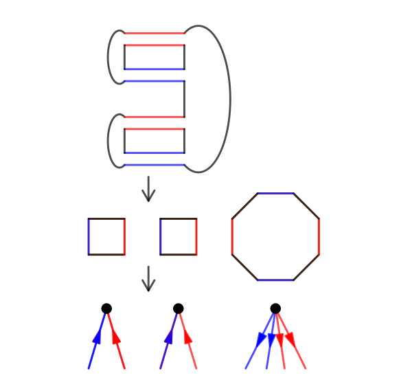
Figure 1: How to read $\rho$ vertices from a ribbon graph.

For $J=1$, the two-point correlation function is

$$N_{1}N_{2}\left(\frac{1}{4\pi k|x_{12}|}\right)^{2}$$ (5.14)

From the powers of $N_{i}$ we know that the $\rho$ graph has one $N_{1}$ vertex and one $N_{2}$ vertex. From the power of $k^{-1}$ we know that the $\rho$ graph has two propagators. There is only one diagram with a single $N_{1}$ vertex, a single $N_{2}$ vertex and two propagators. The diagram is shown in the Figure 2 below. We use a red line for the $z_{1}$ propagator and a blue line for the $z_{2}$ propagator. there is no non-trivial symmetry factor because the two lines in the graph are inequivalent. Evaluating this diagram, we have

$$\frac{1}{4\pi k}\left(-N_{1}\frac{t_{1}t_{2}}{|x_{12}|}\right)\times\frac{1}{4\pi k}\left(-N_{2}\frac{t_{1}t_{2}}{|x_{12}|}\right)$$ (5.15)

This is precisely reproduces the exact result (5.14).

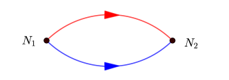
Figure 2: The $\rho$ graph for (5.14).

For a more nontrivial example, consider the two-point correlator for $J=2$

$$N_{1}(N_{1}-1)N_{2}(N_{2}-1)\left(\frac{1}{4\pi k|x_{12}|}\right)^{4}=\left(N_{1}^{2}N_{2}^{2}-N_{1}^{2}N_{2}-N_{2}^{2}N_{1}+N_{1}N_{2}\right)\left(\frac{1}{4\pi k|x_{12}|}\right)^{4}$$ (5.16)

First, consider the signs. From the above answer, there are 4 terms which implies that we need to sum 4 $\rho$ graphs. Each vertex comes with a $-1$. The $N_{1}^{2}N_{2}^{2}$ graph has 4 vertices and $(-1)^{4}=1$, the $N_{1}^{2}N_{2}$ and $N_{1}N_{2}^{2}$ graphs each have three vertices and $(-1)^{3}=-1$ and the $N_{1}N_{2}$ graph has 2 vertices and $(-1)^{2}=1$, so the signs are correct. Each graph has 4 propagators. The graphs are shown in Figure 3 below.

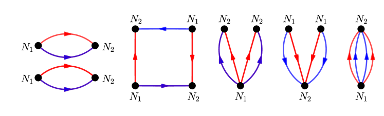
Figure 3: $\rho$ graphs for (5.16)

For this example there are two distinct graphs that contribute to the leading term. The fact that the leading term is a sum of two possible diagrams follows because the leading term comes from the connected (planar) contribution to $\langle{\rm Tr}(Z^{2}){\rm Tr}(Z^{{\dagger}2})$ as well as from the disconnected contribution to $\langle{\rm Tr}(Z)^{2}{\rm Tr}(Z^{{\dagger}})^{2}$. It follows that we need to sum the two diagrams, one connected and one disconnected, that can be formed using two $N_{1}$ vertices, two $N_{2}$ vertices and four propagators.

Finally, consider the $\rho$-description of dual giant gravitons in ABJ(M) theory, which corresponds to the following “effective action”

$$S_{\rm eff} = 4\pi k{\rm Tr}\left(\rho\rho^{\dagger}\right)+N_{1}{\rm Tr}\log\left(M_{1}\right)+N_{2}{\rm Tr}\log\left(M_{2}\right)$$ (5.17)

where

$$(M_{1})_{JK}=\delta_{JK}+\sqrt{\frac{t_{J}t_{K}\bar{\mathcal{Y}}_{K}\cdot\mathcal{Y}_{J}}{\left|x_{KJ}\right|}}\rho_{KJ},\qquad(M_{2})_{KJ}=\delta_{KJ}+\sqrt{\frac{t_{J}t_{K}\bar{\mathcal{Y}}_{K}\cdot\mathcal{Y}_{J}}{\left|x_{KJ}\right|}}\rho_{JK}^{\dagger}$$ (5.18)

Proceeding as above, we find

$$S_{\rm eff} = 4\pi k\left(|z_{1}|^{2}+|z_{2}|^{2}\right)+N_{1}\log\left(1-\frac{t_{1}t_{2}}{|x_{12}|}z_{1}z_{2}\right)+N_{2}\log\left(1-\frac{t_{1}t_{2}}{|x_{12}|}z_{1}^{*}z_{2}^{*}\right)$$ (5.19)

$$= 4\pi k\left(|z_{1}|^{2}+|z_{2}|^{2}\right)-N_{1}\sum_{n=1}^{\infty}{1\over n}\left(\frac{t_{1}t_{2}}{|x_{12}|}z_{1}z_{2}\right)^{n}-N_{2}\sum_{n=1}^{\infty}{1\over n}\left(\frac{t_{1}t_{2}}{|x_{12}|}z_{1}^{*}z_{2}^{*}\right)^{n}$$ (5.20)

All interaction vertices are positive so that giants and the dual giants have opposite signs for the interaction vertices. This makes sense because for the symmetric representation all characters are positive and thus all terms in the correlators of dual giants are positive. The two point correlator is

$$\langle\chi_{J}\left(AB^{{\dagger}}\right)(x_{1})\chi_{J}\left(A^{{\dagger}}B\right)(x_{2})\rangle=\frac{(N_{1}+J-1)!}{(N_{1}-1)!}\frac{(N_{2}+J-1)!}{(N_{2}-1)!}\left(\frac{1}{4\pi k|x_{12}|}\right)^{2J}$$ (5.21)

For $J=2$ we find

$$N_{1}(N_{1}+1)N_{2}(N_{2}+1)\left(\frac{1}{4\pi k|x_{12}|}\right)^{4}=\left(N_{1}^{2}N_{2}^{2}+N_{1}^{2}N_{2}+N_{2}^{2}N_{1}+N_{1}N_{2}\right)\left(\frac{1}{4\pi k|x_{12}|}\right)^{4}$$ (5.22)

All diagrams come with a positive sign which is reproduced by the fact that all vertices in the $\rho$ theory are positive.

6 Large $N_{1}$, $N_{2}$ Saddle Point

The effective action for the $\rho$ theory comes with a factor of $N_{i}$. This is an interesting observation because it implies that the loop expansion of the $\rho$ theory is an expansion in ${1\over N_{i}}$, which is to be contrasted with the description in terms of the original variables, which has the ’t Hooft coupling as the loop expansion parameter. Recall that the dual holographic description of the CFT has ${1\over N_{i}}$ for the loop counting parameter. Motivated by this observation, we will determine the large $N_{i}$ saddle points of the ABJ theory in this section. The analysis is rather interesting: there are two saddles and they are related by parity. To illustrate this, it is enough to consider the simplest case of $Q=2$. Moving to polar-like coordinates $z_{i}=\sqrt{R_{i}}e^{i\theta_{i}}$ the “effective action” (see the first line in (5.12)) becomes

$$S_{\rm eff} = 4\pi k\left(R_{1}+R_{2}\right)-N_{1}\log\left(1-\frac{t_{1}t_{2}}{x_{12}}\sqrt{R_{1}R_{2}}e^{i(\theta_{1}+\theta_{2})}\right)$$ (6.1)

$$- N_{2}\log\left(1-\frac{t_{1}t_{2}}{x_{12}}\sqrt{R_{1}R_{2}}e^{-i(\theta_{1}+\theta_{2})}\right)$$ (6.2)

Notice that, when $N_{1}\neq N_{2}$ the “action” is not hermitian. This will be reflected in the saddle point solutions where we have to analytically continue the angular part. Of course, the fact that the action is complex is not really a problem because this is not really an action: it simply defines the generating function of a class of correlation functions of the theory. There are two saddle points, given by

$$R_{i,\pm} = \frac{1}{8k\pi}\left(N_{1}+N_{2}\pm\sqrt{(N_{1}-N_{2})^{2}+4\chi_{12}^{2}}\right)$$

$$\left(e^{i(\theta_{1}+\theta_{2})}\right)_{\pm} = \frac{1}{2\chi_{12}}\left(N_{1}-N_{2}\pm\sqrt{(N_{1}-N_{2})^{2}+4\chi_{12}^{2}}\right)$$ (6.3)

where $\chi_{12}=\frac{4\pi kx_{12}}{t_{1}t_{2}}$. Note that, unless $N_{1}=N_{2}$, the angle $\theta_{1}+\theta_{2}$ is imaginary. By evaluating the action at the saddle points we must recover the leading large $N$ result for the two point correlation function of giant gravitons. To reproduce the leading order at large $N$ we need only evaluate the action at the saddle point. Issues like the normalization of the measure only contribute at subleading order. After some simplification we find

$$e^{-S_{0+}} = \left(e^{-N_{1}-N_{2}}N_{1}^{N_{1}}N_{2}^{N_{2}}\chi_{12}^{-(N_{1}+N_{2})}\right)e^{-\sqrt{(N_{1}-N_{2})^{2}+4\chi_{12}^{2}}}$$

$$\qquad\qquad\times\left(\frac{\sqrt{(N_{1}-N_{2})^{2}+4\chi_{12}^{2}}+(N_{1}-N_{2})}{\sqrt{(N_{1}-N_{2})^{2}+4\chi_{12}^{2}}-(N_{1}-N_{2})}\right)^{\frac{N_{1}-N_{2}}{2}}$$

$$e^{-S_{0-}} = \left(e^{-N_{1}-N_{2}}N_{1}^{N_{1}}N_{2}^{N_{2}}\chi_{12}^{-(N_{1}+N_{2})}\right)e^{\sqrt{(N_{1}-N_{2})^{2}+4\chi_{12}^{2}}}$$

$$\qquad\qquad\times\left(\frac{\sqrt{(N_{1}-N_{2})^{2}+4\chi_{12}^{2}}-(N_{1}-N_{2})}{\sqrt{(N_{1}-N_{2})^{2}+4\chi_{12}^{2}}+(N_{1}-N_{2})}\right)^{\frac{N_{1}-N_{2}}{2}}$$

These represent the large $N_{i}$ generating functions. To extract a specific correlation function, we must read of the coefficient of a given monomial $t_{1}^{n}t_{2}^{m}$. The $t_{1}t_{2}$ dependence is contained in the $\chi_{12}$ variable. To carry out the series expansion it is useful to define $\chi_{12}=\xi_{12}|N_{1}-N_{2}|$. Assuming that $N_{1}>N_{2}$, the series expansions yield

$$e^{-S_{0-}} = e^{-2N_{2}}\frac{N_{1}^{N_{1}}N_{2}^{N_{2}}}{(N_{1}-N_{2})^{N_{1}-N_{2}}}\frac{1}{(\chi_{12})^{2N_{2}}}$$

$$+e^{-2N_{2}}N_{1}^{N_{1}}N_{2}^{N_{2}}(N_{1}-N_{2})^{-N_{1}+N_{2}-1}\frac{1}{\chi_{12}^{2N_{2}-2}}$$

$$+\frac{1}{2!}e^{-2N_{2}}\frac{N_{1}^{N_{1}}N_{2}^{N_{2}}(N_{1}-N_{2}-1)}{(N_{1}-N_{2})^{N_{1}-(N_{2}-3)}}\frac{1}{(\chi_{12})^{2N_{2}-4}}+\cdots$$

$$e^{-S_{0+}} = e^{-2N_{1}}N_{1}^{N_{1}}N_{2}^{N_{2}}(N_{1}-N_{2})^{N_{1}-N_{2}}\frac{1}{\chi_{12}^{2N_{1}}}$$ (6.6)

$$-e^{-2N_{1}}N_{1}^{N_{1}}N_{2}^{N_{2}}(N_{1}-N_{2})^{N_{1}-N_{2}-1}\frac{1}{\chi_{12}^{2N_{1}-2}}$$

$$+\frac{1}{2!}e^{-2N_{1}}N_{1}^{N_{1}}N_{2}^{N_{2}}(N_{1}-N_{2})^{N_{1}-N_{2}-3}(1+N_{1}-N_{2})\frac{1}{\chi_{12}^{2N_{1}-4}}+\cdots$$

These results reproduce the correct leading $N_{1},N_{2}$ behavior of the giant graviton two point function. Indeed, taking the coefficient of the third order term from the first expansion, for example, we have

$$\frac{1}{2!}e^{-2N_{2}}\frac{N_{1}^{N_{1}}N_{2}^{N_{2}}(N_{1}-N_{2}-1)}{(N_{1}-N_{2})^{N_{1}-(N_{2}-3)}} \approx e^{-2N_{2}}\frac{N_{1}^{N_{1}}N_{2}^{N_{2}}}{(N_{1}-(N_{2}-2))^{N_{1}-(N_{2}-2)}2!}$$ (6.7)

$$\approx \frac{N_{1}!N_{2}!}{(N_{1}-(N_{2}-2))!2!}$$ (6.8)

where we used Stirling’s approximation in the last approximation. Notice that the two answers are related by $e^{-S_{0-}}=\left.(-1)^{N_{1}-N_{2}}e^{-S_{0+}}\right|_{N_{1}\leftrightarrow N_{2}}$. The first series thus represents the correct large $N_{1}\geq N_{2}$ expansion while the second represents the correct large $N_{2}\geq N_{1}$ expansion. The swap $N_{1}\leftrightarrow N_{2}$ is accomplished by parity. Thus, the two saddles are related by a parity transformation. This is exactly what we expect from the breaking of the discrete $Z_{2}$ parity symmetry when $N_{1}\neq N_{2}$.

7 Discussion

The basic result of this article is an efficient approach to the computation of correlation functions involving operators corresponding to giant gravitons and dual giant gravitons, as well as traces, in the ABJM and ABJ theories. This generalizes results developed in the setting of ${\cal N}=4$ super Yang-Mills theory[14, 15]. The derivation of this effective description makes use of a novel identity following from character orthogonality to obtain an integral representation of certain projection operators used to define Schur polynomials. Then, after integrating over the original matrix variables and performing a Hubbard-Stratonovich transformation, one obtains a description in terms of a $K\times K$ matrix for a collection of $K$ giant or dual giant gravitons. The resulting effective descriptions have ${1\over N}$ as the loop counting parameter. Since ${1\over N}$ controls quantum corrections in the dual gravitational description, this strongly suggests the effective description is relevant for understanding the holography of the ABJM and ABJ theories.

There are a number of immediate directions that warrant further study. Our analysis has been restricted to the free field theory. It would be interesting to consider loop corrections. Loop corrections to restricted Schur polynomials in ABJM theory have been considered in [30]. In addition, the analysis of [14] has suggested that integrability maybe present for correlation functions involving two determinants and a single trace operator. A study of loop corrections may establish a similar result in the ABJM/ABJ theories.

Thanks to the fact that there are many different composite adjoint matrices that can be constructed from the ABJM/ABJ fields, there are many different restricted Schur polynomials one could consider[19]. It would be interesting to develop effective descriptions for this large class of operators.

Acknowledgements

This work is supported by the South African Research Chairs Initiative of the Department of Science and Technology and National Research Foundation of South Africa as well as by funds received from the National Institute for Theoretical Physics (NITheP).

Appendix A Fermion Measure Conventions

In this Appendix we spell out our conventions for the fermion measure. The conventions of this paper agree with those of our last paper [15]. Namely, we use

$$\int d\bar{\psi}_{N}\cdots d\bar{\psi}_{1}\int d\psi^{1}\cdots d\psi^{N}\bar{\psi}_{1}\psi^{1}\cdots\bar{\psi}_{N}\psi^{N}=\left(-1\right)^{N}$$ (A.1)

With this convention the Gaussian integral is given by

$$\int d^{N}\bar{\psi}d^{N}\psi\,e^{-\bar{\psi}M\psi}=\det\left(M\right)$$ (A.2)

Another commonly used convention, which differs by a phase at most, is

$$\int d\psi^{1}d\bar{\psi}_{1}\cdots d\psi^{N}d\bar{\psi}_{N}\,\bar{\psi}_{1}\psi^{1}\cdots\bar{\psi}_{N}\psi^{N}=1$$ (A.3)

Had we used this convention, the Gaussian integral would become

$$\int d^{N}\psi d^{N}\bar{\psi}\,e^{\bar{\psi}M\psi}=\det\left(M\right)$$ (A.4)

With this convention some equations would differ by a signs. For example, the sign factor in (2.24) disappears

$$\int[d\chi d\bar{\chi}][d\psi d\bar{\psi}]\bar{\chi}_{b_{1}}\chi^{a}\cdots\bar{\chi}_{b_{n}}\chi^{a_{n}}\left(\bar{\chi}\cdot\chi\right)^{N_{1}-n}\bar{\psi}_{\beta_{1}}\psi^{\alpha_{1}}\cdots\bar{\psi}_{\beta_{n}}\psi^{\alpha_{n}}\left(\sum_{i}\bar{\psi}_{i}\psi^{i}\right)^{N_{2}-n}\\ =\left(N_{1}-n\right)!\left(N_{2}-n\right)!\sum_{\sigma,\rho\in S_{n}}\chi_{(1^{n})}\left(\sigma\right)\chi_{(1^{n})}\left(\rho\right)\sigma_{\mathbf{\beta}}^{\mathbf{\alpha}}\sigma_{\mathbf{b}}^{\mathbf{a}}$$ (A.5)

The generating function (2.28) would become

$$t_{1}^{2i_{1}}\cdots t_{Q}^{2i_{Q}}\left\langle\chi_{(1^{i_{1}})}\left(x_{1}\right)\cdots\chi_{(1^{i_{Q}})}\left(x_{Q}\right)\mathcal{O}\right\rangle=\int d\phi^{I}d\phi^{\dagger I}\int\prod_{K}^{Q}[d\chi_{K}d\bar{\chi}_{K}][d\psi_{K}d\bar{\psi}_{K}]\\ e^{-k\int d^{3}x\left[\partial_{\mu}\phi^{I}\partial^{\mu}\phi^{\dagger I}-\frac{1}{k}\sum_{K=1}^{Q}\delta(x-x_{K})\left(\bar{\psi}_{K}\cdot\psi_{K}+\bar{\chi}_{K}\cdot\chi_{K}+t_{K}\bar{\chi}_{K}\mathcal{Z}_{K}\psi_{K}-t_{K}\bar{\psi}\bar{\mathcal{Z}}_{K}\chi\right)\right]}\mathcal{O}\left(\phi^{I},\phi^{I\dagger}\right)$$ (A.6)

where $\int\prod_{K=1}^{Q}[d\psi_{K}d\bar{\psi}_{K}]\equiv\int\prod_{K=1}^{Q}\prod_{\alpha=1}^{N}d\psi_{K}^{\alpha}d\bar{\psi}_{K\alpha}$. Note the sign change before the delta function. Because of (A.4), the sign difference would disappear in (2.30) after the integration over the fermion fields is performed. This is expected since our results should be independent of these conventions.

References

[1]
N. Beisert et al.,
“Review of AdS/CFT Integrability: An Overview,”
Lett. Math. Phys. 99, 3 (2012)
doi:10.1007/s11005-011-0529-2
[arXiv:1012.3982 [hep-th]].
[2]
J. M. Maldacena,
“The Large N limit of superconformal field theories and supergravity,”
Int. J. Theor. Phys. 38, 1113 (1999)
[Adv. Theor. Math. Phys. 2, 231 (1998)]
doi:10.1023/A:1026654312961, 10.4310/ATMP.1998.v2.n2.a1
[hep-th/9711200].
[3]
S. S. Gubser, I. R. Klebanov and A. M. Polyakov,
“Gauge theory correlators from noncritical string theory,”
Phys. Lett. B 428, 105 (1998)
doi:10.1016/S0370-2693(98)00377-3
[hep-th/9802109].
[4]
E. Witten,
“Anti-de Sitter space and holography,”
Adv. Theor. Math. Phys. 2, 253 (1998)
doi:10.4310/ATMP.1998.v2.n2.a2
[hep-th/9802150].
[5]
N. Gromov, V. Kazakov and P. Vieira,
“Exact Spectrum of Anomalous Dimensions of Planar N=4 Supersymmetric Yang-Mills Theory,”
Phys. Rev. Lett. 103, 131601 (2009)
doi:10.1103/PhysRevLett.103.131601
[arXiv:0901.3753 [hep-th]].
[6]
V. Balasubramanian, M. Berkooz, A. Naqvi and M. J. Strassler,
“Giant gravitons in conformal field theory,”
JHEP 0204, 034 (2002)
doi:10.1088/1126-6708/2002/04/034
[hep-th/0107119].
[7]
D. Berenstein,
“Shape and holography: Studies of dual operators to giant gravitons,”
Nucl. Phys. B 675, 179 (2003)
doi:10.1016/j.nuclphysb.2003.10.004
[hep-th/0306090].
[8]
S. Corley, A. Jevicki and S. Ramgoolam,
“Exact correlators of giant gravitons from dual N=4 SYM theory,”
Adv. Theor. Math. Phys. 5, 809 (2002)
doi:10.4310/ATMP.2001.v5.n4.a6
[hep-th/0111222],
S. Corley and S. Ramgoolam,
“Finite factorization equations and sum rules for BPS correlators in N=4 SYM theory,”
Nucl. Phys. B 641, 131 (2002)
doi:10.1016/S0550-3213(02)00573-4
[hep-th/0205221].
[9]
O. Aharony, Y. E. Antebi, M. Berkooz and R. Fishman,
“’Holey sheets’: Pfaffians and subdeterminants as D-brane operators in large N gauge theories,”
JHEP 0212, 069 (2002)
doi:10.1088/1126-6708/2002/12/069
[hep-th/0211152].
[10]
H. Lin, O. Lunin and J. M. Maldacena,
“Bubbling AdS space and 1/2 BPS geometries,”
JHEP 0410, 025 (2004)
doi:10.1088/1126-6708/2004/10/025
[hep-th/0409174].
[11]
O. Aharony, O. Bergman, D. L. Jafferis and J. Maldacena,
“N=6 superconformal Chern-Simons-matter theories, M2-branes and their gravity duals,”
JHEP 0810, 091 (2008)
doi:10.1088/1126-6708/2008/10/091
[arXiv:0806.1218 [hep-th]].
[12]
O. Aharony, O. Bergman and D. L. Jafferis,
“Fractional M2-branes,”
JHEP 0811, 043 (2008)
doi:10.1088/1126-6708/2008/11/043
[arXiv:0807.4924 [hep-th]].
[13]
D. Bombardelli, A. Cavaglià, D. Fioravanti, N. Gromov and R. Tateo,
“The full Quantum Spectral Curve for ,”
JHEP 1709 (2017) 140
doi:10.1007/JHEP09(2017)140
[arXiv:1701.00473 [hep-th]].
[14]
Y. Jiang, S. Komatsu and E. Vescovi,
“Structure Constants in SYM at Finite Coupling as Worldsheet -Function,”
arXiv:1906.07733 [hep-th],
Y. Jiang, S. Komatsu and E. Vescovi,
“Exact Three-Point Functions of Determinant Operators in Planar N=4 Supersymmetric Yang-Mills Theory,”
arXiv:1907.11242 [hep-th].
[15]
G. Chen, R. de Mello Koch, M. Kim and H. J. R. Van Zyl,
“Absorption of closed strings by giant gravitons,”
arXiv:1908.03553 [hep-th].
[16]
T. K. Dey,
“Exact Large -charge Correlators in ABJM Theory,”
JHEP 1108, 066 (2011)
doi:10.1007/JHEP08(2011)066
[arXiv:1105.0218 [hep-th]].
[17]
S. Chakrabortty and T. K. Dey,
“Correlators of Giant Gravitons from dual ABJ(M) Theory,”
JHEP 1203, 062 (2012)
doi:10.1007/JHEP03(2012)062
[arXiv:1112.6299 [hep-th]].
[18]
P. Caputa and B. A. E. Mohammed,
“From Schurs to Giants in ABJ(M),”
JHEP 1301, 055 (2013)
doi:10.1007/JHEP01(2013)055
[arXiv:1210.7705 [hep-th]].
[19]
R. de Mello Koch, B. A. E. Mohammed, J. Murugan and A. Prinsloo,
“Beyond the Planar Limit in ABJM,”
JHEP 1205, 037 (2012)
doi:10.1007/JHEP05(2012)037
[arXiv:1202.4925 [hep-th]].
[20]
J. Pasukonis and S. Ramgoolam,
“Quivers as Calculators: Counting, Correlators and Riemann Surfaces,”
JHEP 1304, 094 (2013)
doi:10.1007/JHEP04(2013)094
[arXiv:1301.1980 [hep-th]],
P. Mattioli and S. Ramgoolam,
“Gauge Invariants and Correlators in Flavoured Quiver Gauge Theories,”
Nucl. Phys. B 911, 638 (2016)
doi:10.1016/j.nuclphysb.2016.08.021
[arXiv:1603.04369 [hep-th]].
[21]
T. Nishioka and T. Takayanagi,
“Fuzzy Ring from M2-brane Giant Torus,”
JHEP 0810, 082 (2008)
doi:10.1088/1126-6708/2008/10/082
[arXiv:0808.2691 [hep-th]].
[22]
D. Berenstein and J. Park,
“The BPS spectrum of monopole operators in ABJM: Towards a field theory description of the giant torus,”
JHEP 1006, 073 (2010)
doi:10.1007/JHEP06(2010)073
[arXiv:0906.3817 [hep-th]].
[23]
M. M. Sheikh-Jabbari and J. Simon,
“On Half-BPS States of the ABJM Theory,”
JHEP 0908, 073 (2009)
doi:10.1088/1126-6708/2009/08/073
[arXiv:0904.4605 [hep-th]].
[24]
A. Hamilton, J. Murugan, A. Prinsloo and M. Strydom,
“A Note on dual giant gravitons in ,”
JHEP 0904 (2009) 132
doi:10.1088/1126-6708/2009/04/132
[arXiv:0901.0009 [hep-th]].
[25]
D. Giovannoni, J. Murugan and A. Prinsloo,
“The Giant graviton on - another step towards the emergence of geometry,”
JHEP 1112, 003 (2011)
doi:10.1007/JHEP12(2011)003
[arXiv:1108.3084 [hep-th]].
[26]
S. Hirano, C. Kristjansen and D. Young,
“Giant Gravitons on and their Holographic Three-point Functions,”
JHEP 1207, 006 (2012)
doi:10.1007/JHEP07(2012)006
[arXiv:1205.1959 [hep-th]].
[27]
Y. Lozano and A. Prinsloo,
“S S3 geometries in ABJM and giant gravitons,”
JHEP 1304, 148 (2013)
doi:10.1007/JHEP04(2013)148
[arXiv:1303.3748 [hep-th]].
[28]
R. Gopakumar. Open-closed-open string duality - 2010. talk at Second Joburg Workshop on String Theory.
http://neo.phys.wits.ac.za/workshop2/pdfs/rajesh.pdf
[29]
W. Lederman, “Introduction to Group Characters,” Cambridge University Press, 1977.
[30]
R. de Mello Koch, R. Kreyfelt and S. Smith,
“Heavy Operators in Superconformal Chern-Simons Theory,”
Phys. Rev. D 90, no. 12, 126009 (2014)
doi:10.1103/PhysRevD.90.126009
[arXiv:1410.0874 [hep-th]].