On the nodal distance between two Keplerian trajectories with a common focus

Abstract

We study the possible values of the nodal distance $\delta_{\rm nod}$ between two non-coplanar Keplerian trajectories ${\cal A},{\cal A}^{\prime}$ with a common focus. In particular, given ${\cal A}^{\prime}$ and assuming it is bounded, we compute optimal lower and upper bounds for $\delta_{\rm nod}$ as functions of a selected pair of orbital elements of ${\cal A}$, when the other elements vary. This work arises in the attempt to extend to the elliptic case the optimal estimates for the orbit distance given in [5] in case of a circular trajectory ${\cal A}^{\prime}$. These estimates are relevant to understand the observability of celestial bodies moving (approximately) along ${\cal A}$ when the observer trajectory is (close to) ${\cal A}^{\prime}$.

1 Introduction

The computation of the distance $d_{\rm min}$ between two Keplerian trajectories ${\cal A}$, ${\cal A}^{\prime}$ with a common focus, also called orbit distance, is relevant for different purposes in Celestial Mechanics. Several authors introduced efficient methods to compute $d_{\rm min}$, e.g. [11], [8], [3], [4]. Small values of $d_{\rm min}$ are relevant for the assessment of the hazard of near-Earth asteroids with the Earth [10], [2], or for the detection of conjunctions between satellites of the Earth [6], [1]. On the other hand, we may wish to check whether $d_{\rm min}$ can assume large values, because in this case it is more difficult to observe a small celestial body moving along ${\cal A}$ from a point following ${\cal A}^{\prime}$.

In [5] the authors studied the range of the values of the orbit distance $d_{\rm min}$ between the trajectory ${\cal A}^{\prime}$ of the Earth, assumed to be circular, and the possible trajectory ${\cal A}$ of a near-Earth asteroid, as a function of selected pairs of orbital elements. The results have been used to detect some observational biases in the known population of near-Earth asteroids (NEAs). We would like to extend these results to the case of an elliptic trajectory ${\cal A}^{\prime}$. This generalization seems to be difficult because $d_{\rm min}$ is implicitely defined, and because two local minima of the distance between a point of ${\cal A}$ and a point of ${\cal A}^{\prime}$ may exchange their role as the orbit distance, see [5]. Therefore, as a first step in this direction, we investigate the range of the values of the nodal distance $\delta_{\rm nod}$, which is defined explicitely by equation (1). The distance $\delta_{\rm nod}$ is defined only when the two trajectories are not coplanar, and is similar to $d_{\rm min}$ for some aspects: $\delta_{\rm nod}=0$ if and only if $d_{\rm min}=0$, moreover the absolute values of the ascending and descending nodal distances may exchange their role as the nodal distance. We also have $d_{\rm min}\leq\delta_{\rm nod}$, thus the nodal distance gives us an upper bound to the orbit distance.

The ascending and descending nodal distances have also been used in [7] to define linking coefficients as functions of the orbital elements and to estimate the orbit distance. A lower bound for the orbit distance is also given in [9].

This paper is organized as follows. In Section 2 we introduce the nodal distance $\delta_{\rm nod}$ and show some basic properties. In Section 3 we present the main results, that is optimal bounds for $\delta_{\rm nod}$: first we deal with the case of an eccentric trajectory ${\cal A}^{\prime}$, with $e^{\prime}\in(0,1)$, then we consider the particular case $e^{\prime}=0$ and compare the results with the ones in [5]. In Section 4 we show an application of the results to the known population of NEAs. Finally, in Section 5, we discuss the analogies and the differences between the optimal upper bounds of $\delta_{\rm nod}$ and $d_{\rm min}$ on the basis of numerical computations.

2 Preliminary definitions and basic properties

2.1 Mutual orbital elements

Given two non-coplanar Keplerian trajectories ${\cal A},{\cal A}^{\prime}$ with a common focus, we define the cometary mutual elements

$${\cal E}_{M}=(q,e,q^{\prime},e^{\prime},I_{M},\omega_{M},\omega_{M}^{\prime})$$

as follows: $q,e$ and $q^{\prime},e^{\prime}$ are the pericenter distance and the eccentricity of the two trajectories, $I_{M}$ is the mutual inclination between the two orbital planes and $\omega_{M},\omega_{M}^{\prime}$ are the angles between the ascending mutual node and the pericenters of ${\cal A}$ and ${\cal A}^{\prime}$, see Figure 1.

Figure 1: The mutual orbital elements $I_{M},\omega_{M},\omega_{M}^{\prime}$.

The map

$$\Phi:(E,E^{\prime})\rightarrow{\cal E}_{M},$$

from the usual cometary elements

$$E=(q,e,I,\Omega,\omega),\qquad E^{\prime}=(q^{\prime},e^{\prime},I^{\prime},\Omega^{\prime},\omega^{\prime})$$

of ${\cal A}$, ${\cal A}^{\prime}$, to the mutual elements, is not injective: there are infinitely many configurations leading to the same mutual position of the two orbits. We can select a unique set of orbital elements $(E,E^{\prime})$ in each counter-image $\Phi^{-1}\left({\cal E}_{M}\right)$ as follows:

$$E=(q,e,I_{M},0,\omega_{M}),\qquad E^{\prime}=(q^{\prime},e^{\prime},0,0,\omega_{M}^{\prime}).$$

This corresponds to computing the usual cometary elements with respect to the mutual reference frame $Oxyz$, with the $x$-axis along the mutual nodal line, oriented towards the ascending mutual node, assuming that ${\cal A}^{\prime}$ lies on the $xy$ plane. Another possible choice is

$$E=(q,e,I_{M},-\omega_{M}^{\prime},\omega_{M}),\qquad E^{\prime}=(q^{\prime},e^{\prime},0,0,0),$$

where we choose the reference $Oxyz$ with the $x$-axis along the apsidal line of ${\cal A}^{\prime}$, oriented towards its pericenter. In this way, for a given choice of the pericenter distance $q^{\prime}$ and the eccentricity $e^{\prime}$ of ${\cal A}^{\prime}$, we can vary all the other mutual elements by changing only the elements of ${\cal A}$.

For simplicity, from now on we shall drop the subscript in $I_{M},\omega_{M},\omega_{M}^{\prime}$ and the adjective ‘mutual’ referred to the nodes and to the nodal distances. We assume that $q^{\prime}>0$ and $e^{\prime}\in[0,1)$ are given, and let the other mutual elements vary in the following ranges:

$$0<q\leq q_{\rm max},\qquad 0\leq e\leq 1,\qquad 0<I<\pi,\qquad 0\leq\omega,\omega^{\prime}<2\pi,$$

for a given $q_{\rm max}>0$.

Moreover, we admit that the considered functions of the mutual orbital elements attain the values $+\infty$ and $-\infty$, when there exists an infinite limit for the value of such functions.

2.2 The nodal distance

Let us set

$$\begin{split}&r_{\scaleto{+}{5pt}}=\frac{q(1+e)}{1+e\cos\omega},\qquad r_{\scaleto{-}{5pt}}=\frac{q(1+e)}{1-e\cos\omega},\\ &r_{\scaleto{+}{5pt}}^{\prime}=\frac{q^{\prime}(1+e^{\prime})}{1+e^{\prime}\cos\omega^{\prime}},\quad\ \ r_{\scaleto{-}{5pt}}^{\prime}=\frac{q^{\prime}(1+e^{\prime})}{1-e^{\prime}\cos\omega^{\prime}}\\ \end{split}$$

and introduce the ascending and descending nodal distances:

$$d_{\rm nod}^{+}=r_{\scaleto{+}{5pt}}^{\prime}-r_{\scaleto{+}{5pt}},\qquad d_{\rm nod}^{-}=r_{\scaleto{-}{5pt}}^{\prime}-r_{\scaleto{-}{5pt}}.$$

Definition 1.

We define the (minimal) nodal distance $\delta_{\rm nod}$ as the minimum between the absolute values of the ascending and descending nodal distances:

$$\delta_{\rm nod}=\min\bigl{\{}|d_{\rm nod}^{+}|,|d_{\rm nod}^{-}|\bigr{\}}.$$ (1)

Note that $\delta_{\rm nod}$ does not depend on the mutual inclination $I$.

Remark 1.

The transformations

$$\begin{split}&(\omega,\omega^{\prime})\mapsto(\pi-\omega,\pi-\omega^{\prime}),\qquad(\omega,\omega^{\prime})\mapsto(\pi+\omega,\pi-\omega^{\prime}),\\ &(\omega,\omega^{\prime})\mapsto(2\pi-\omega,\omega^{\prime}),\qquad\quad\ (\omega,\omega^{\prime})\mapsto(\omega,2\pi-\omega^{\prime})\\ \end{split}$$

leave the values of $\delta_{\rm nod}$ unchanged.

By the previous remark we get all the possible values of $\delta_{\rm nod}$ even if we restrict $\omega,\omega^{\prime}$ to the following ranges:

$$0\leq\omega\leq\pi/2,\qquad 0\leq\omega^{\prime}\leq\pi.$$ (2)

We prove the following elementary facts:

Lemma 1.

Assuming $(\omega,\omega^{\prime})\in[0,\pi]\times[0,\pi]$, the ascending nodal distance $d_{\rm nod}^{+}$ is a non-increasing function of $\omega$ and a non-decreasing function of $\omega^{\prime}$. In the same domain the descending nodal distance $d_{\rm nod}^{-}$ is a non-decreasing function of $\omega$ and a non-increasing function of $\omega^{\prime}$. Moreover, both $d_{\rm nod}^{+}$ and $d_{\rm nod}^{-}$ are non-increasing functions of $e$.

Proof.

We only need to compute the following derivatives:

$$\begin{split}&\frac{\partial d_{\rm nod}^{+}}{\partial\omega}=-\frac{e\sin\omega}{(1+e\cos\omega)}r_{\scaleto{+}{5pt}},\qquad\frac{\partial d_{\rm nod}^{+}}{\partial\omega^{\prime}}=\frac{e^{\prime}\sin\omega^{\prime}}{(1+e^{\prime}\cos\omega^{\prime})}r_{\scaleto{+}{5pt}}^{\prime},\\ &\frac{\partial d_{\rm nod}^{-}}{\partial\omega}=\frac{e\sin\omega}{(1-e\cos\omega)}r_{\scaleto{-}{5pt}},\qquad\frac{\partial d_{\rm nod}^{-}}{\partial\omega^{\prime}}=-\frac{e^{\prime}\sin\omega^{\prime}}{(1-e^{\prime}\cos\omega^{\prime})}r_{\scaleto{-}{5pt}}^{\prime},\\ &\frac{\partial d_{\rm nod}^{+}}{\partial e}=-\frac{q(1-\cos\omega)}{(1+e\cos\omega)^{2}},\qquad\frac{\partial d_{\rm nod}^{-}}{\partial e}=-\frac{q(1+\cos\omega)}{(1-e\cos\omega)^{2}}.\\ \end{split}$$

∎

We shall use this notation for the semi-latus rectum and for the apocenter distance:

$$p=q(1+e),\qquad p^{\prime}=q^{\prime}(1+e^{\prime}),\qquad Q=\frac{q(1+e)}{1-e},\qquad Q^{\prime}=\frac{q^{\prime}(1+e^{\prime})}{1-e^{\prime}}.$$

Moreover, we shall employ the variables

$$\xi=e\cos\omega,\qquad\xi^{\prime}=e^{\prime}\cos\omega^{\prime}.$$

Definition 2.

We consider the following linking configurations between the trajectories ${\cal A},{\cal A}^{\prime}$:

• internal nodes: the nodes of ${\cal A}$ are internal to those of ${\cal A}^{\prime}$, that is $d_{\rm nod}^{+},d_{\rm nod}^{-}>0$. A sufficient condition for this case is $Q<q^{\prime}$;

• external nodes: the nodes of ${\cal A}$ are external to those of ${\cal A}^{\prime}$ (possibly located at infinity), that is $d_{\rm nod}^{+},d_{\rm nod}^{-}<0$. A sufficient condition for this case is $q>Q^{\prime}$;

• linked orbits: ${\cal A}$ and ${\cal A}^{\prime}$ are topologically linked, that is $d_{\rm nod}^{+}<0<d_{\rm nod}^{-}$, or $d_{\rm nod}^{-}<0<d_{\rm nod}^{+}$;

• crossing orbits: ${\cal A}$ and ${\cal A}^{\prime}$ have at least one point in common, that is $d_{\rm nod}^{+}d_{\rm nod}^{-}=0$.

Assume $q^{\prime}>0$ and $e^{\prime}\in[0,1)$ are given. We introduce the functions

$$\begin{split}&\delta_{\rm int}(q,e,\omega,\omega^{\prime})=\min\{d_{\rm nod}^{+},d_{\rm nod}^{-}\},\\ &\delta_{\rm ext}(q,e,\omega,\omega^{\prime})=\min\{-d_{\rm nod}^{+},-d_{\rm nod}^{-}\},\\ &\delta_{\rm link}^{(i)}(q,e,\omega,\omega^{\prime})=\min\{-d_{\rm nod}^{+},d_{\rm nod}^{-}\},\\ &\delta_{\rm link}^{(ii)}(q,e,\omega,\omega^{\prime})=\min\{d_{\rm nod}^{+},-d_{\rm nod}^{-}\},\\ &\delta_{\rm link}(q,e,\omega,\omega^{\prime})=\max\{\delta_{\rm link}^{(i)},\delta_{\rm link}^{(ii)}\}.\\ \end{split}$$

The linking configurations depend on the sign of these functions as described below.

Lemma 2.

Given the vector $(q,e,\omega,\omega^{\prime})$, we have

• internal nodes if and only if $\delta_{\rm int}(q,e,\omega,\omega^{\prime})>0$,

• external nodes if and only if $\delta_{\rm ext}(q,e,\omega,\omega^{\prime})>0$,

• linked orbits if and only if $\delta_{\rm link}(q,e,\omega,\omega^{\prime})>0$,

• crossing orbits if and only if $\delta_{\rm int}=\delta_{\rm ext}=\delta_{\rm link}=0$ at $(q,e,\omega,\omega^{\prime})$.

Moreover,

$$\delta_{\rm nod}=\max\{\delta_{\rm int},\delta_{\rm ext},\delta_{\rm link}\}.$$ (3)

Proof.

Properties $a)$ - $d)$ follow immediately from Definition 2. Relation (3) follows from the fact that the linking configurations are mutually exclusive, therefore at least one of the expressions $\delta_{\rm int},\delta_{\rm ext},\delta_{\rm link}$ must be non-negative, and if one of these is strictly positive, then the other two are strictly negative.

∎

3 Optimal bounds for the nodal distance

In this section we state and prove optimal bounds for $\delta_{\rm nod}$ as functions of selected pairs of orbital elements. For the case $e^{\prime}=0$ we also compare the results with the ones obtained in [5] for the orbit distance $d_{\rm min}$.

3.1 Bounds for $\delta_{\rm nod}$ when $e^{\prime}\in(0,1)$

Assume $q^{\prime}>0$ and $e^{\prime}\in(0,1)$ are given. First we present the optimal lower and upper bounds for $\delta_{\rm nod}$ as functions of $(q,\omega)$.

Proposition 1.

Let ${\cal D}_{1}=\{(e,\omega^{\prime}):0\leq e\leq 1,0\leq\omega^{\prime}\leq\pi\}$, ${\cal D}_{2}=\{(q,\omega):0<q\leq q_{\rm max},0\leq\omega\leq{\pi}/{2}\}$. For each choice of $(q,\omega)\in{\cal D}_{2}$ we have

$$\displaystyle\min_{(e,\omega^{\prime})\in{\cal D}_{1}}\delta_{\rm nod}=\max\bigl{\{}0,\ell^{\omega}_{\rm int},\ell^{\omega}_{\rm ext}\bigr{\}},$$ (4)

$$\displaystyle\max_{(e,\omega^{\prime})\in{\cal D}_{1}}\delta_{\rm nod}=\max\bigl{\{}u^{\omega}_{\rm int},u^{\omega}_{\rm ext},u^{\omega}_{\rm link}\bigr{\}},$$ (5)

where

$$\ell^{\omega}_{\rm int}(q,\omega)=q^{\prime}-\frac{2q}{1-\cos\omega},\qquad\ell^{\omega}_{\rm ext}(q,\omega)=q-Q^{\prime},$$

$$u^{\omega}_{\rm int}(q,\omega)=p^{\prime}-q,$$

$$u^{\omega}_{\rm ext}(q,\omega)=\min\Bigl{\{}\frac{2q}{1-\cos\omega}-\frac{p^{\prime}}{1-\hat{\xi}^{\prime}_{*}},\ \frac{2q}{1+\cos\omega}-q^{\prime}\Bigr{\}},$$

with

$$\hat{\xi}^{\prime}_{*}=\min\{\xi_{*}^{\prime},e^{\prime}\},$$

where

$$\xi^{\prime}_{*}(q,\omega)=\frac{4q\cos\omega}{p^{\prime}\sin^{2}\omega+\sqrt{p^{\prime 2}\sin^{4}\omega+16q^{2}\cos^{2}\omega}},$$

and

$$u^{\omega}_{\rm link}(q,\omega)=\min\left\{Q^{\prime}-\frac{q(1+\hat{e}_{*})}{1+\hat{e}_{*}\cos\omega},\frac{2q}{1-\cos\omega}-q^{\prime}\right\},$$ (6)

with

$$\hat{e}_{*}=\max\bigl{\{}0,\min\{e_{*},1\}\bigr{\}},$$

where

$$e_{*}(q,\omega)=\frac{2(p^{\prime}-q(1-e^{\prime 2}))}{q(1-e^{\prime 2})+\sqrt{q^{2}(1-e^{\prime 2})^{2}+4p^{\prime}\cos^{2}\omega(p^{\prime}-q(1-e^{\prime 2}))}}.$$

Proof.

We prove some preliminary facts.

Lemma 3.

The following properties hold:

• for each $(q,\omega)\in{\cal D}_{2}$ and $(e,\omega^{\prime})\in{\cal D}_{1}$ we have

  $$\delta_{\rm int}(q,e,\omega,\omega^{\prime})\geq\delta_{\rm int}(q,1,\omega,\pi)=\ell^{\omega}_{\rm int}(q,\omega),$$ (7)

  $$\delta_{\rm ext}(q,e,\omega,\omega^{\prime})\geq\delta_{\rm ext}(q,0,\omega,\pi)=\ell^{\omega}_{\rm ext}(q,\omega),$$ (8)

  therefore, given $(q,\omega)\in{\cal D}_{2}$, we have internal (resp. external) nodes for each $(e,\omega^{\prime})\in{\cal D}_{1}$ if and only if $\ell^{\omega}_{\rm int}(q,\omega)>0$ (resp. $\ell^{\omega}_{\rm ext}(q,\omega)>0$);

• if $(q,\omega)$ is such that $\ell^{\omega}_{\rm int}(q,\omega)\leq 0$ and $\ell^{\omega}_{\rm ext}(q,\omega)\leq 0$, then there exists $(e,\omega^{\prime})\in{\cal D}_{1}$ such that $d_{\rm nod}^{+}d_{\rm nod}^{-}=0$, i.e. there exists $(e,\omega^{\prime})$ corresponding to a crossing configuration.

Proof.

We prove the bounds (7), (8) by observing that for each $(q,\omega)\in{\cal D}_{2}$ and $(e,\omega^{\prime})\in{\cal D}_{1}$ we have

$$\begin{split}\delta_{\rm int}&\geq\min\biggl{\{}\min_{\omega^{\prime}\in[0,\pi]}r_{\scaleto{+}{5pt}}^{\prime}-\max_{e\in[0,1]}r_{\scaleto{+}{5pt}},\min_{\omega^{\prime}\in[0,\pi]}r_{\scaleto{-}{5pt}}^{\prime}-\max_{e\in[0,1]}r_{\scaleto{-}{5pt}}\biggr{\}}\cr&=\min\{r_{\scaleto{+}{5pt}}^{\prime}|_{\omega^{\prime}=0}-r_{\scaleto{+}{5pt}}|_{e=1},r_{\scaleto{-}{5pt}}^{\prime}|_{\omega^{\prime}=\pi}-r_{\scaleto{-}{5pt}}|_{e=1}\}=q^{\prime}-\frac{2q}{1-\cos\omega}\cr\end{split}$$

and

$$\begin{split}\delta_{\rm ext}&\geq\min\biggl{\{}\min_{e\in[0,1]}r_{\scaleto{+}{5pt}}-\max_{\omega^{\prime}\in[0,\pi]}r_{\scaleto{+}{5pt}}^{\prime},\min_{e\in[0,1]}r_{\scaleto{-}{5pt}}-\max_{\omega^{\prime}\in[0,\pi]}r_{\scaleto{-}{5pt}}^{\prime}\biggr{\}}\cr&=\min\{r_{\scaleto{+}{5pt}}|_{e=0}-r_{\scaleto{+}{5pt}}^{\prime}|_{\omega^{\prime}=\pi},r_{\scaleto{-}{5pt}}|_{e=0}-r_{\scaleto{-}{5pt}}^{\prime}|_{\omega^{\prime}=0}\}=q-Q^{\prime}.\cr\end{split}$$

We conclude the proof of i) using properties a), b) in Lemma 3. To prove ii) we note that

$$\delta_{\rm int}(q,0,\omega,\pi/2)=p^{\prime}-q,\qquad\delta_{\rm ext}(q,0,\omega,\pi/2)=q-p^{\prime}$$

for each $(q,\omega)\in{\cal D}_{2}$. Therefore, either they are both zero and there is a crossing for $(e,\omega^{\prime})=(0,\pi/2)$, or they are different from zero and opposite and, since we are assuming that $\ell^{\omega}_{\rm int},\ell^{\omega}_{\rm ext}\leq 0$ at $(q,\omega)$, by continuity there exists $(e,\omega^{\prime})\in{\cal D}_{1}$ corresponding to a crossing configuration.

∎

We continue the proof of Proposition 1.

Lower bound: we prove relation (4) by observing that, by i) of Lemma 3, if $\ell^{\omega}_{\rm int}(q,\omega)>0$ we can have only internal nodes for each $(e,\omega^{\prime})\in{\cal D}_{1}$. Therefore $\min_{(e,\omega^{\prime})\in{\cal D}_{1}}\delta_{\rm nod}(q,\omega)=\min_{(e,\omega^{\prime})\in{\cal D}_{1}}\delta_{\rm int}(q,\omega)=\ell^{\omega}_{\rm int}(q,\omega)$ and $\delta_{\rm ext}(q,e,\omega,\omega^{\prime})$, $\delta_{\rm link}(q,e,\omega,\omega^{\prime})<0$ for each $(e,\omega^{\prime})\in{\cal D}_{1}$. In particular we have $\ell^{\omega}_{\rm ext}(q,\omega)<0$. In a similar way, if $\ell^{\omega}_{\rm ext}(q,\omega)>0$ we can have only external nodes for each $(e,\omega^{\prime})\in{\cal D}_{1}$. Therefore $\min_{(e,\omega^{\prime})\in{\cal D}_{1}}\delta_{\rm nod}(q,\omega)=\min_{(e,\omega^{\prime})\in{\cal D}_{1}}\delta_{\rm ext}(q,\omega)=\ell^{\omega}_{\rm ext}(q,\omega)$ and $\delta_{\rm int}(q,e,\omega,\omega^{\prime})$, $\delta_{\rm link}(q,e,\omega,\omega^{\prime})<0$ for each $(e,\omega^{\prime})\in{\cal D}_{1}$. In particular we have $\ell^{\omega}_{\rm int}(q,\omega)<0$. Finally, if $\ell^{\omega}_{\rm int}(q,\omega)\leq 0$ and $\ell^{\omega}_{\rm ext}(q,\omega)\leq 0$, by ii) of Lemma 3 there exists $(e,\omega^{\prime})\in{\cal D}_{1}$ corresponding to a crossing configuration, therefore $\min_{(e,\omega^{\prime})\in{\cal D}_{1}}\delta_{\rm nod}(q,\omega)=0$. The previous discussion yields relation (4).

Upper bound: by Lemma 1 both $d_{\rm nod}^{+}$ and $d_{\rm nod}^{-}$ are non-increasing functions of $e$, therefore also $\delta_{\rm int}$ is, and we have

$$\delta_{\rm int}(q,e,\omega,\omega^{\prime})\leq\delta_{\rm int}(q,0,\omega,\omega^{\prime})$$

for each $(q,\omega)\in{\cal D}_{2}$ and $(e,\omega^{\prime})\in{\cal D}_{1}$. By the same lemma, $d_{\rm nod}^{+}$ is non-decreasing with $\omega^{\prime}$, while $d_{\rm nod}^{-}$ is non-increasing, whatever the value of $e$. Moreover, for $e=0$ we have $d_{\rm nod}^{+}=d_{\rm nod}^{-}$ if and only if

$$\frac{p^{\prime}\xi^{\prime}}{1-\xi^{\prime 2}}=0$$

with $\xi^{\prime}=e^{\prime}\cos\omega^{\prime}$, that is for $\omega^{\prime}={\pi}/{2}$. We conclude that for each $(q,\omega)\in{\cal D}_{2}$ the maximal value of $\delta_{\rm int}$ over ${\cal D}_{1}$ is

$$u^{\omega}_{\rm int}(q,\omega)=\delta_{\rm int}(q,0,\omega,\pi/2)=p^{\prime}-q.$$

We also observe that by Lemma 1 we have

$$\delta_{\rm ext}(q,e,\omega,\omega^{\prime})\leq\delta_{\rm ext}(q,1,\omega,\omega^{\prime}).$$

Moreover, by the same lemma, $-d_{\rm nod}^{+}$ is non-increasing with $\omega^{\prime}$ while $-d_{\rm nod}^{-}$ is non-decreasing, whatever the value of $e$. Let us set

$$\begin{split}&D_{+}(0)=\left.d_{\rm nod}^{+}\right|_{e=1,\omega^{\prime}=0}=q^{\prime}-\frac{2q}{1+\cos\omega},\\ &D_{-}(0)=\left.d_{\rm nod}^{-}\right|_{e=1,\omega^{\prime}=0}=Q^{\prime}-\frac{2q}{1-\cos\omega},\\ &D_{+}(\pi)=\left.d_{\rm nod}^{+}\right|_{e=1,\omega^{\prime}=\pi}=Q^{\prime}-\frac{2q}{1+\cos\omega},\\ &D_{-}(\pi)=\left.d_{\rm nod}^{-}\right|_{e=1,\omega^{\prime}=\pi}=q^{\prime}-\frac{2q}{1-\cos\omega}.\\ \end{split}$$

Figure 2: Possible behavior of $-d_{\rm nod}^{+}$ and $-d_{\rm nod}^{-}$ as functions of $\omega^{\prime}$.

We consider the three cases depicted in Figure 2:

• $-D_{+}(\pi)>-D_{-}(\pi)$, which corresponds to

  $$Q^{\prime}-q^{\prime}<-4q\frac{\cos\omega}{\sin^{2}\omega};$$

• $-D_{+}(0)\geq-D_{-}(0)$ and $-D_{+}(\pi)\leq-D_{-}(\pi)$, which correspond to

  $$Q^{\prime}-q^{\prime}\geq 4q\frac{\cos\omega}{\sin^{2}\omega};$$

• $-D_{+}(0)<-D_{-}(0)$, which corresponds to

  $$Q^{\prime}-q^{\prime}<4q\frac{\cos\omega}{\sin^{2}\omega}.$$

Indeed case a) is impossible, because $Q^{\prime}\geq q^{\prime}$ and $\omega\in[0,\pi/2]$. In case b) the maximal value of $\delta_{\rm ext}$ is attained for $e=1$ and $\omega^{\prime}$ such that $d_{\rm nod}^{+}=d_{\rm nod}^{-}$, that is when

$$\frac{p^{\prime}\xi^{\prime}}{1-\xi^{\prime 2}}=\frac{2q\cos\omega}{\sin^{2}\omega},$$ (9)

with $\xi^{\prime}=e^{\prime}\cos\omega^{\prime}$. The solution of (9) is

$$\xi_{*}^{\prime}(q,\omega)=\frac{4q\cos\omega}{p^{\prime}\sin^{2}\omega+\sqrt{p^{\prime 2}\sin^{4}\omega+16q^{2}\cos^{2}\omega}},$$ (10)

for which we find

$$\omega_{*}^{\prime}=\arccos\frac{\xi_{*}^{\prime}}{e^{\prime}},$$

if $\xi_{*}^{\prime}\leq e^{\prime}$. In case c) equation $d_{\rm nod}^{+}=d_{\rm nod}^{-}$ has no real solution for $\omega^{\prime}$, that is $\xi_{*}^{\prime}>e^{\prime}$, and the maximal value of $\delta_{\rm ext}$ is given by $-d_{\rm nod}^{+}$ with $e=1$ and $\omega^{\prime}=0$.

We introduce the cut-off

$$\hat{\xi}_{*}^{\prime}=\min\{\xi_{*}^{\prime},e^{\prime}\}$$ (11)

and define

$$\hat{\omega}_{*}^{\prime}=\arccos(\hat{\xi}_{*}^{\prime}/e^{\prime}).$$

From the previous discussion we obtain that the maximal value of $\delta_{\rm ext}$ over ${\cal D}_{1}$ is given by

$$\begin{split}u^{\omega}_{\rm ext}(q,\omega)&=\min\left\{\left.-d_{\rm nod}^{-}\right|_{e=1,\omega^{\prime}=\hat{\omega}^{\prime}_{*}},\left.-d_{\rm nod}^{+}\right|_{e=1,\omega^{\prime}=0}\right\}\cr&=\min\Bigl{\{}\frac{2q}{1-\cos\omega}-\frac{p^{\prime}}{1-\hat{\xi}_{*}^{\prime}},\frac{2q}{1+\cos\omega}-q^{\prime}\Bigr{\}}.\cr\end{split}$$

Finally, we consider the function $\delta_{\rm link}$ and examine $\delta_{\rm link}^{(i)}$ and $\delta_{\rm link}^{(ii)}$ separately. We can not select a priori a value of the eccentricity $e$ that maximizes $\delta_{\rm link}$, as we did before. However, we can do this for $\omega^{\prime}$, in fact by Lemma 1 both $-d_{\rm nod}^{+}$ and $d_{\rm nod}^{-}$ are non-increasing functions of $\omega^{\prime}$, therefore also $\delta_{\rm link}^{(i)}$ is. Therefore, for each fixed value of $q,e,\omega$ the maximal value of $\delta_{\rm link}^{(i)}$ is attained for $\omega^{\prime}=0$. By a similar argument we obtain that for each fixed value of $q,e,\omega$ the maximal value of $\delta_{\rm link}^{(ii)}$ is attained for $\omega^{\prime}=\pi$.

We observe that $d_{\rm nod}^{+}=-d_{\rm nod}^{-}$ if and only if

$$q(1+e)(1-\xi^{\prime 2})=p^{\prime}(1-e^{2}\cos^{2}\omega)$$ (12)

where $\xi^{\prime}=e^{\prime}\cos\omega^{\prime}$. Both for $\omega^{\prime}=0$ and for $\omega^{\prime}=\pi$ equation (12) becomes

$$q(1+e)(1-e^{\prime 2})=p^{\prime}(1-e^{2}\cos^{2}\omega),$$

that gives the eccentricity

$$e_{*}(q,\omega)=\frac{2(p^{\prime}-q(1-e^{\prime 2}))}{q(1-e^{\prime 2})+\sqrt{q^{2}(1-e^{\prime 2})^{2}+4p^{\prime}\cos^{2}\omega(p^{\prime}-q(1-e^{\prime 2}))}}$$ (13)

We observe that $e_{*}$ can attain negative values, or values larger than 1. For this reason we introduce the cut-off

$$\hat{e}_{*}(q,\omega)=\max\{0,\min\{e_{*}(q,\omega),1\}\}.$$ (14)

By Lemma 1, $-d_{\rm nod}^{+}$ is non-decreasing with $e$, while $d_{\rm nod}^{-}$ is non-increasing, whatever the value of $\omega^{\prime}$. Let us set

$$\begin{split}&D^{(i)}_{+}(0)=\left.d_{\rm nod}^{+}\right|_{\omega^{\prime}=0,e=0}=q^{\prime}-q,\\ &D^{(i)}_{-}(0)=\left.d_{\rm nod}^{-}\right|_{\omega^{\prime}=0,e=0}=Q^{\prime}-q,\\ &D^{(i)}_{+}(1)=\left.d_{\rm nod}^{+}\right|_{\omega^{\prime}=0,e=1}=q^{\prime}-\frac{2q}{1+\cos\omega},\\ &D^{(i)}_{-}(1)=\left.d_{\rm nod}^{-}\right|_{\omega^{\prime}=0,e=1}=Q^{\prime}-\frac{2q}{1-\cos\omega}.\\ \end{split}$$

Figure 3: Possible behavior of $-d_{\rm nod}^{+}$ and $d_{\rm nod}^{-}$ as functions of $e$.

We consider the three cases

• $-D^{(i)}_{+}(0)>D^{(i)}_{-}(0)$, which corresponds to

  $$Q^{\prime}+q^{\prime}<2q;$$

• $-D^{(i)}_{+}(0)\leq D^{(i)}_{-}(0)$ and $-D^{(i)}_{+}(1)\geq D^{(i)}_{-}(1)$, which correspond to

  $$2q\leq Q^{\prime}+q^{\prime}\leq\frac{4q}{\sin^{2}\omega};$$

• $-D^{(i)}_{+}(1)<D^{(i)}_{-}(1)$, which corresponds to

  $$Q^{\prime}+q^{\prime}>\frac{4q}{\sin^{2}\omega}.$$

Therefore, the maximal value of $\delta_{\rm link}^{(i)}$ over ${\cal D}_{1}$ is given by

$$\min\left\{\left.d_{\rm nod}^{-}\right|_{\omega^{\prime}=0,e=\hat{e}_{*}},\left.-d_{\rm nod}^{+}\right|_{\omega^{\prime}=0,e=1}\right\}=\min\left\{Q^{\prime}-\frac{q(1+\hat{e}_{*})}{1-\hat{e}_{*}\cos\omega},\frac{2q}{1+\cos\omega}-q^{\prime}\right\}.$$

To compute a bound for $\delta_{\rm link}^{(ii)}$ we observe that $d_{\rm nod}^{+}$ is non-increasing with $e$, while $-d_{\rm nod}^{-}$ is non-decreasing. Let us set

$$\begin{split}&D^{(ii)}_{+}(0)=\left.d_{\rm nod}^{+}\right|_{\omega^{\prime}=\pi,e=0}=Q^{\prime}-q,\\ &D^{(ii)}_{-}(0)=\left.d_{\rm nod}^{-}\right|_{\omega^{\prime}=\pi,e=0}=q^{\prime}-q,\\ &D^{(ii)}_{+}(1)=\left.d_{\rm nod}^{+}\right|_{\omega^{\prime}=\pi,e=1}=Q^{\prime}-\frac{2q}{1+\cos\omega},\\ &D^{(ii)}_{-}(1)=\left.d_{\rm nod}^{-}\right|_{\omega^{\prime}=\pi,e=1}=q^{\prime}-\frac{2q}{1-\cos\omega}.\\ \end{split}$$

Figure 4: Possible behavior of $d_{\rm nod}^{+}$ and $-d_{\rm nod}^{-}$ as functions of $e$.

We consider the three cases

• $D^{(ii)}_{+}(0)<-D^{(ii)}_{-}(0)$, which corresponds to

  $$Q^{\prime}+q^{\prime}<2q;$$

• $D^{(ii)}_{+}(0)\geq-D^{(ii)}_{-}(0)$ and $D^{(ii)}_{+}(1)\leq-D^{(ii)}_{-}(1)$, which correspond to

  $$2q\leq Q^{\prime}+q^{\prime}\leq\frac{4q}{\sin^{2}\omega};$$

• $D^{(ii)}_{+}(1)>-D^{(ii)}_{-}(1)$, which corresponds to

  $$Q^{\prime}+q^{\prime}>\frac{4q}{\sin^{2}\omega}.$$ (15)

Therefore, the maximal value of $\delta_{\rm link}^{(ii)}$ over ${\cal D}_{1}$ is given by

$$\min\left\{\left.d_{\rm nod}^{+}\right|_{\omega^{\prime}=\pi,e=\hat{e}_{*}},\left.-d_{\rm nod}^{-}\right|_{\omega^{\prime}=\pi,e=1}\right\}=\min\left\{Q^{\prime}-\frac{q(1+\hat{e}_{*})}{1+\hat{e}_{*}\cos\omega},\frac{2q}{1-\cos\omega}-q^{\prime}\right\},$$

where $\hat{e}_{*}$ is defined as in (14). We conclude that the maximal value of $\delta_{\rm link}$ over ${\cal D}_{1}$ is given by

$$\begin{split}u^{\omega}_{\rm link}(q,\omega)&=\max\left\{\min\Bigl{\{}Q^{\prime}-\frac{q(1+\hat{e}_{*})}{1-\hat{e}_{*}\cos\omega},\frac{2q}{1+\cos\omega}-q^{\prime}\Bigr{\}},\ \min\Bigl{\{}Q^{\prime}-\frac{q(1+\hat{e}_{*})}{1+\hat{e}_{*}\cos\omega},\frac{2q}{1-\cos\omega}-q^{\prime}\Bigr{\}}\right\}\\ &=\min\left\{Q^{\prime}-\frac{q(1+\hat{e}_{*})}{1+\hat{e}_{*}\cos\omega},\frac{2q}{1-\cos\omega}-q^{\prime}\right\},\end{split}$$

where the last equality holds because $\omega\in[0,{\pi}/{2}]$. In particular, the maximal value is attained by $\delta_{\rm link}^{(ii)}$.

We conclude the proof of relation (5) using (3) and the optimal bounds

$$\delta_{\rm int}(q,e,\omega,\omega^{\prime})\leq u^{\omega}_{\rm int}(q,\omega),\quad\delta_{\rm ext}(q,e,\omega,\omega^{\prime})\leq u^{\omega}_{\rm ext}(q,\omega),\quad\delta_{\rm link}(q,e,\omega,\omega^{\prime})\leq u^{\omega}_{\rm link}(q,\omega).$$

∎

In Figure 5 we show the graphic of $\max_{(e,\omega^{\prime})\in{\cal D}_{1}}\delta_{\rm nod}(q,\omega)$ for different values of $e^{\prime}$, with $q^{\prime}=1$. Using Remark 1 we can extend by symmetry the graphic of $\max_{(e,\omega^{\prime})\in{\cal D}_{1}}\delta_{\rm nod}(q,\omega)$ to the set $(0,q_{\rm max}]\times[0,2\pi)$.

  

  

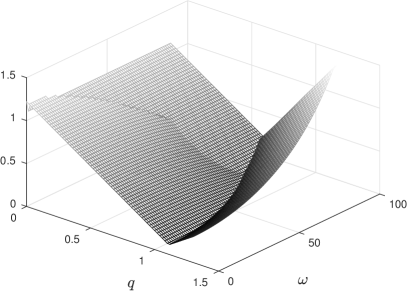
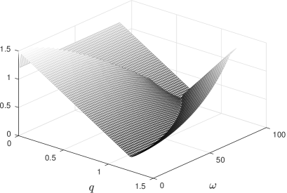
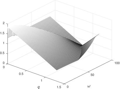
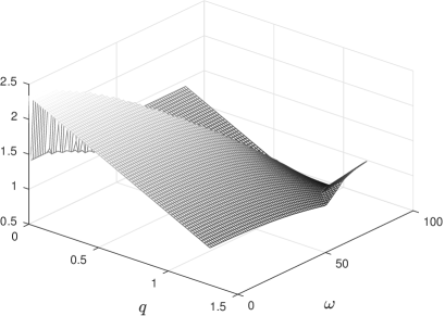
Figure 5: Graphics of $(q,\omega)\mapsto\max_{(e,\omega^{\prime})\in{\cal D}_{1}}\delta_{\rm nod}(q,\omega)$ for $e^{\prime}=0.1$ (top left), $e^{\prime}=0.2$ (top right), $e^{\prime}=0.3$ (bottom left), $e^{\prime}=0.4$ (bottom right). Here we set $q^{\prime}=1$.

Proposition 2.

The zero level curves of $\ell^{\omega}_{\rm int},\ell^{\omega}_{\rm ext},u^{\omega}_{\rm int},u^{\omega}_{\rm ext}$ divide the plane $(q,\omega)$ into regions where different linking configurations are allowed. Moreover, $u^{\omega}_{\rm ext}(q,\omega)=0$ is a piecewise smooth curve with only one component, a portion of which is a vertical segment with $q={p^{\prime}}/{2}$.

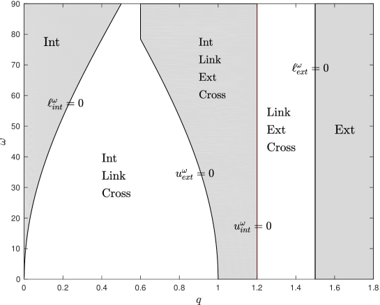
Figure 6: Regions with different linking configurations in the plane $(q,\omega)$ for $q^{\prime}=1$ and $e^{\prime}=0.2$.

Proof.

By Lemma 3, given $(q,\omega)\in{\cal D}_{2}$, we have internal nodes for each $(e,\omega^{\prime})\in{\cal D}_{1}$ if and only if $\ell^{\omega}_{\rm int}(q,\omega)>0$, therefore the region where only internal nodes are possible is delimited on the right by the curve $\ell^{\omega}_{\rm int}(q,\omega)=0$. In a similar way, the region with only external nodes is delimited on the left by $\ell^{\omega}_{\rm ext}(q,\omega)=0$.

Moreover, we have internal nodes for some choice of $(e,\omega^{\prime})$ if and only if $u^{\omega}_{\rm int}(q,\omega)>0$. In a similar way, we have external nodes (resp. linked orbits) for some choice of $(e,\omega^{\prime})$ if and only if $u^{\omega}_{\rm ext}(q,\omega)>0$ (resp. $u^{\omega}_{\rm link}(q,\omega)>0$).

We prove the following result.

Lemma 4.

The curve

$$u^{\omega}_{\rm link}(q,\omega)=0,$$

delimiting the region where linked orbits are possible, has two connected components, and coincides with the curve

$$\{\ell^{\omega}_{\rm int}(q,\omega)=0\}\cup\{\ell^{\omega}_{\rm ext}(q,\omega)=0\}.$$

Proof.

If $(q,\omega)$ is such that

$$Q^{\prime}-\frac{q(1+\hat{e}_{*})}{1+\hat{e}_{*}\cos\omega}=0,$$ (16)

then

$$\frac{2q}{1-\cos\omega}-q^{\prime}>\frac{2q}{1+\cos\omega}-Q^{\prime}=\frac{2q}{1+\cos\omega}-\frac{q(1+\hat{e}_{*})}{1+\hat{e}_{*}\cos\omega}\geq 0,$$

because $\frac{q(1+e)}{1+e\cos\omega}$ is increasing with $e$. We prove that (16) is equivalent to

$$Q^{\prime}-q=0$$ (17)

From relations (13), (14) we deduce that $\hat{e}_{*}(q,\omega)=0$ if and only if $p^{\prime}\leq q(1-e^{\prime 2})$, that is if

$$q\geq\frac{q^{\prime}}{1-e^{\prime}}.$$ (18)

Since $q=Q^{\prime}$ fulfills (18), then (17) implies (16). To prove the converse first we observe that relation (16) implies

$$\frac{1}{2}Q^{\prime}\leq q\leq Q^{\prime}.$$ (19)

If $\hat{e}_{*}=0$, i.e. if $e_{*}\leq 0$, then relations (16) and (17) are the same. Otherwise $e_{*}>0$. If $e_{*}\in(0,1]$ then $e_{*}$ is defined so that it satisfies $d_{\rm nod}^{+}=-d_{\rm nod}^{-}$ with $\omega^{\prime}=\pi$, therefore using (16) we have

$$Q^{\prime}-\frac{q(1+e_{*})}{1+e_{*}\cos\omega}=\frac{q(1+e_{*})}{1-e_{*}\cos\omega}-q^{\prime}=0,$$ (20)

from which we obtain

$$e_{*}=\frac{q^{\prime}-Q^{\prime}}{(q^{\prime}+Q^{\prime})\cos\omega}<0,$$

giving a contradiction. If $e_{*}>1$ then (15) holds. Therefore, either $\cos\omega=1$ and relations (16) and (17) are the same, or we have $4q\leq 2Q^{\prime}\sin^{2}\omega<2Q^{\prime}$, that contradicts (19).

We conclude that, in this case, $u^{\omega}_{\rm link}(q,\omega)=Q^{\prime}-q$, and the curve $u^{\omega}_{\rm link}(q,\omega)=0$ has a connected component corresponding to $\ell^{\omega}_{\rm ext}(q,\omega)=0$.

On the other hand, if $(q,\omega)$ is such that

$$\frac{2q}{1-\cos\omega}-q^{\prime}=0,$$

then

$$Q^{\prime}-\frac{q(1+\hat{e}_{*})}{1+\hat{e}_{*}\cos\omega}>q^{\prime}-\frac{q(1+\hat{e}_{*})}{1+\hat{e}_{*}\cos\omega}=\frac{2q}{1-\cos\omega}-\frac{q(1+\hat{e}_{*})}{1+\hat{e}_{*}\cos\omega}\geq 0.$$

Therefore, in this case, $u^{\omega}_{\rm link}(q,\omega)=\frac{2q}{1-\cos\omega}-q^{\prime}$, and the curve $u^{\omega}_{\rm link}(q,\omega)=0$ has another connected component coinciding with $\ell^{\omega}_{\rm int}(q,\omega)=0$.

∎

Now we describe the shape of the curve $u^{\omega}_{\rm ext}(q,\omega)=0$. First we observe that

$$\frac{2q}{1-\cos\omega}-\frac{p^{\prime}}{1-\hat{\xi}_{*}^{\prime}}=\max\{F_{1},F_{2}\},$$ (21)

where

$$F_{1}(q,\omega)=\frac{2q}{1-\cos\omega}-\frac{p^{\prime}}{1-\xi_{*}^{\prime}},\qquad F_{2}(q,\omega)=\frac{2q}{1-\cos\omega}-\frac{p^{\prime}}{1-e^{\prime}}.$$

The relation

$$F_{1}(q,\omega)=0$$ (22)

corresponds to

$$q=p^{\prime}/2.$$ (23)

In fact $\xi_{*}^{\prime}$ is defined so that it satisfies $d_{\rm nod}^{+}=d_{\rm nod}^{-}$ with $e=1$, therefore, if (22) holds, we have

$$\frac{2q}{1-\cos\omega}-\frac{p^{\prime}}{1-\xi_{*}^{\prime}}=\frac{2q}{1+\cos\omega}-\frac{p^{\prime}}{1+\xi_{*}^{\prime}}=0,$$

from which we obtain (23). On the other hand, substituting $q=p^{\prime}/2$ into (10) we obtain

$$\xi_{*}^{\prime}=\frac{2\cos\omega}{\sin^{2}\omega+\sqrt{\sin^{4}\omega+4\cos^{2}\omega}}=\frac{2\cos\omega}{1-\cos^{2}\omega+\sqrt{(1-\cos^{2}\omega)^{2}+4\cos^{2}\omega}}=\cos\omega,$$ (24)

that yields (22).

Since $F_{1}(q,\pi/2)=2q-p^{\prime}$, by continuity we obtain

$$F_{1}(q,\omega)>0\qquad\mbox{if}\ \ q>p^{\prime}/2,$$ (25)

$$F_{1}(q,\omega)<0\qquad\mbox{if}\ \ q<p^{\prime}/2,$$ (26)

for each $\omega\in[0,\pi/2]$. We also note that

$$F_{2}(q,\omega)<0\qquad\mbox{if}\ \ q<p^{\prime}/2,\ \omega\in[\arccos e^{\prime},\pi/2].$$ (27)

Using (21), (25) we obtain that

$$\frac{2q}{1-\cos\omega}-\frac{p^{\prime}}{1-\hat{\xi}_{*}^{\prime}}>0\qquad\mbox{if}\ \ q>p^{\prime}/2,$$

so that, for such values of $q$, $u^{\omega}_{\rm ext}=0$ corresponds to $\frac{2q}{1+\cos\omega}-q^{\prime}=0$.

On the other hand, we can prove that

$$u^{\omega}_{\rm ext}(q,\omega)<0\qquad\mbox{if}\ \ q<p^{\prime}/2,$$

therefore the curve $u^{\omega}_{\rm ext}=0$ does not intersect the region with $q<p^{\prime}/2$. In fact, by (26), (27) we obtain that

$$\max\{F_{1},F_{2}\}<0\qquad\mbox{if}\ \ \omega\in[\arccos e^{\prime},\pi/2],$$

and we can easily check that, for such values of $q$,

$$\frac{2q}{1+\cos\omega}-q^{\prime}<0\qquad\mbox{if}\ \ \omega\in[0,\arccos e^{\prime}).$$

Finally, we prove that, if $q=p^{\prime}/2$, we have

$$u^{\omega}_{\rm ext}(q,\omega)=0\qquad\mbox{if and only if}\qquad\omega\in[\arccos e^{\prime},\pi/2].$$

Assume that $q=p^{\prime}/2$. If $\omega\in(\arccos e^{\prime},\pi/2]$ then $u^{\omega}_{\rm ext}(q,\omega)=0$. In fact, in this case, from (24) we obtain $\hat{\xi}_{*}^{\prime}=\cos\omega$, so that

$$\qquad\frac{2q}{1-\cos\omega}-\frac{p^{\prime}}{1-\hat{\xi}_{*}^{\prime}}=0$$

and

$$\frac{2q}{1+\cos\omega}-q^{\prime}=\frac{p^{\prime}}{1+\cos\omega}-\frac{p^{\prime}}{1+e^{\prime}}>0.$$

On the other hand, if $\omega\in[0\arccos e^{\prime})$ then

$$u^{\omega}_{\rm ext}(q,\omega)<0,$$

because in this case

$$\frac{2q}{1+\cos\omega}-q^{\prime}<0.$$

Finally, if $\omega=\arccos e^{\prime}$, we have $\hat{\xi}_{*}^{\prime}=\cos\omega=e^{\prime}$, so that

$$\frac{2q}{1-\cos\omega}-\frac{p^{\prime}}{1-\hat{\xi}_{*}^{\prime}}=\frac{2q}{1+\cos\omega}-q^{\prime}=0.$$ (28)

We conclude that the curve $u^{\omega}_{\rm ext}(q,\omega)=0$ is composed by the vertical segment $\{(q,\omega):q=p^{\prime}/2,\ \omega\in[\arccos e^{\prime},\pi/2]\}$ and by the curve $\{(q,\omega)\in{\cal D}_{2}:\frac{2q}{1+\cos\omega}-q^{\prime}=0,\ q>p^{\prime}/2\}$. These two portions of the curve $u^{\omega}_{\rm ext}=0$ meet in the point $(q,\omega)=(p^{\prime}/2,\arccos e^{\prime})$ and therefore they form a unique connected component. The proof of Proposition 2 is concluded.

∎

Remark 2.

There can not exist $(q,\omega)\in{\cal D}_{2}$ such that we have linked orbits for each $(e,\omega^{\prime})\in{\cal D}_{1}$, unlike the case of internal and external nodes.

Proof.

If $\delta_{\rm link}(q,e,\omega,\omega^{\prime})>0$ for each $(e,\omega^{\prime})\in{\cal D}_{1}$ then in particular $u^{\omega}_{\rm link}(q,\omega)>0$, and this corresponds to $\ell^{\omega}_{\rm int},\ell^{\omega}_{\rm ext}<0$ at $(q,\omega)$, so that, by ii) of Lemma 3, there exists $(e,\omega^{\prime})$ corresponding to a crossing configuration, that yields a contradiction.

∎

In Figure 6 we show the possible linking configurations for $q^{\prime}=1$ and $e^{\prime}=0.2$.

In the next statement we present the optimal lower and upper bounds for $\delta_{\rm nod}$ as functions of $(q,e)$.

Proposition 3.

Let ${\cal D}_{3}=\{(\omega,\omega^{\prime}):0\leq\omega\leq{\pi}/{2},0\leq\omega^{\prime}<\pi\}$, ${\cal D}_{4}=\{(q,e):0<q\leq q_{\rm max},0\leq e\leq 1\}$. For each choice of $(q,e)\in{\cal D}_{4}$ we have

$$\displaystyle\min_{(\omega,\omega^{\prime})\in{\cal D}_{3}}\delta_{\rm nod}=\max\Bigl{\{}0,\ell^{\>e}_{\rm int},\ell^{\>e}_{\rm ext}\Bigr{\}},$$ (29)

$$\displaystyle\max_{(\omega,\omega^{\prime})\in{\cal D}_{3}}\delta_{\rm nod}=\max\{u^{\>e}_{\rm link},|p^{\prime}-q(1+e)|\},$$ (30)

where

$$\ell^{\>e}_{\rm int}(q,e)=q^{\prime}-\frac{q(1+e)}{1-e},\qquad\ell^{\>e}_{\rm ext}(q,e)=q-Q^{\prime},$$

$$u^{\>e}_{\rm link}(q,e)=\min\left\{\frac{q(1+e)}{1-e}-q^{\prime},Q^{\prime}-q\right\}.$$

Proof.

We prove some preliminary facts.

Lemma 5.

The following properties hold:

• for each $(q,e)\in{\cal D}_{4}$ and $(\omega,\omega^{\prime})\in{\cal D}_{3}$ we have

  $$\delta_{\rm int}(q,e,\omega,\omega^{\prime})\geq\delta_{\rm int}(q,e,0,\pi)=\ell^{\>e}_{\rm int}(q,e),$$ (31)

  $$\delta_{\rm ext}(q,e,\omega,\omega^{\prime})\geq\delta_{\rm ext}(q,e,0,\pi)=\ell^{\>e}_{\rm ext}(q,e),$$ (32)

  therefore, given $(q,e)\in{\cal D}_{4}$, we have internal (resp. external) nodes for each $(\omega,\omega^{\prime})\in{\cal D}_{3}$ if and only if $\ell^{\>e}_{\rm int}(q,e)>0$ (resp. $\ell^{\>e}_{\rm ext}(q,e)>0$);

• if $(q,e)$ is such that $\ell^{\>e}_{\rm int}(q,e)\leq 0$ and $\ell^{\>e}_{\rm ext}(q,e)\leq 0$, then there exists $(\omega,\omega^{\prime})\in{\cal D}_{3}$ such that $d_{\rm nod}^{+}d_{\rm nod}^{-}=0$.

Proof.

We prove the bounds (31), (32) by observing that for each $(q,e)\in{\cal D}_{4}$ and $(\omega,\omega^{\prime})\in{\cal D}_{3}$ we have

$$\begin{split}\delta_{\rm int}&\geq\min\Bigl{\{}\min_{\omega^{\prime}\in[0,\pi]}r_{\scaleto{+}{5pt}}^{\prime}-\max_{\omega\in[0,\pi/2]}r_{\scaleto{+}{5pt}},\min_{\omega^{\prime}\in[0,\pi]}r_{\scaleto{-}{5pt}}^{\prime}-\max_{\omega\in[0,\pi/2]}r_{\scaleto{-}{5pt}}\Bigr{\}}\cr&=\min\{r_{\scaleto{+}{5pt}}^{\prime}|_{\omega^{\prime}=0}-r_{\scaleto{+}{5pt}}|_{\omega=\pi/2},r_{\scaleto{-}{5pt}}^{\prime}|_{\omega^{\prime}=\pi}-r_{\scaleto{-}{5pt}}|_{\omega=0}\}=q^{\prime}-\frac{q(1+e)}{1-e}\cr\end{split}$$

and

$$\begin{split}\delta_{\rm ext}&\geq\min\Bigl{\{}\min_{\omega\in[0,\pi/2]}r_{\scaleto{+}{5pt}}-\max_{\omega^{\prime}\in[0,\pi]}r_{\scaleto{+}{5pt}}^{\prime},\min_{\omega\in[0,\pi/2]}r_{\scaleto{-}{5pt}}-\max_{\omega^{\prime}\in[0,\pi]}r_{\scaleto{-}{5pt}}^{\prime}\Bigr{\}}\cr&=\min\{r_{\scaleto{+}{5pt}}|_{\omega=0}-r_{\scaleto{+}{5pt}}^{\prime}|_{\omega^{\prime}=\pi},r_{\scaleto{-}{5pt}}|_{\omega=\pi/2}-r_{\scaleto{-}{5pt}}^{\prime}|_{\omega^{\prime}=0}\}=q-Q^{\prime}.\cr\end{split}$$

We conclude the proof of i) using properties a), b) in Lemma 3. To prove ii) we note that

$$\delta_{\rm int}(q,e,\pi/2,\pi/2)=q^{\prime}-q,\qquad\delta_{\rm ext}(q,e,\pi/2,\pi/2)=q-q^{\prime}.$$

Therefore, either they are both zero and there is a crossing for $(\omega,\omega^{\prime})=(\pi/2,\pi/2)$, or they are different from zero and opposite and, since we are assuming that $\ell^{\>e}_{\rm int},\ell^{\>e}_{\rm ext}\leq 0$ at $(q,e)$, by continuity there exists $(\omega,\omega^{\prime})\in{\cal D}_{3}$ corresponding to a crossing configuration.

∎

We also prove the following result.

Lemma 6.

Let us consider the function

$$D(\xi,\xi^{\prime};p,p^{\prime})=\min\Bigl{\{}\frac{p^{\prime}}{1+\xi^{\prime}}-\frac{p}{1+\xi},\frac{p^{\prime}}{1-\xi^{\prime}}-\frac{p}{1-\xi}\Bigr{\}}$$

defined for $(\xi,\xi^{\prime})\in{\cal D}:=(-1,1)\times(-1,1)$, depending on the parameters $p,p^{\prime}>0$. Then we have

$$\sup_{(\xi,\xi^{\prime})\in{\cal D}}D(\xi,\xi^{\prime};p,p^{\prime})=\left\{\begin{array}[]{ll}p^{\prime}-p=D(0,0;p,p^{\prime})&\mbox{ if }\ p^{\prime}\geq p,\cr\displaystyle\frac{p^{\prime}-p}{2}=\limsup_{(\xi,\xi^{\prime})\to\pm(1,1)}D(\xi,\xi^{\prime};p,p^{\prime})&\mbox{ if }\ p^{\prime}<p.\cr\end{array}\right.$$

Proof.

Let us set

$$D^{+}(\xi,\xi^{\prime};p,p^{\prime})=\frac{p^{\prime}}{1+\xi^{\prime}}-\frac{p}{1+\xi}\ \quad\mbox{and}\ \quad D^{-}(\xi,\xi^{\prime};p,p^{\prime})=\frac{p^{\prime}}{1-\xi^{\prime}}-\frac{p}{1-\xi}.$$

For each $\xi\in(-1,1)$, $D^{+}$ is a non-increasing function of $\xi^{\prime}$, while $D^{-}$ is non-decreasing. Moreover,

$$\lim_{\xi^{\prime}\to-1^{+}}D^{+}(\xi,\xi^{\prime};p,p^{\prime})=+\infty,\qquad\lim_{\xi^{\prime}\to 1^{-}}D^{+}(\xi,\xi^{\prime};p,p^{\prime})=\frac{p^{\prime}}{2}-\frac{p}{1+\xi},$$

and

$$\lim_{\xi^{\prime}\to-1^{+}}D^{-}(\xi,\xi^{\prime};p,p^{\prime})=\frac{p^{\prime}}{2}-\frac{p}{1-\xi},\qquad\lim_{\xi^{\prime}\to 1^{-}}D^{-}(\xi,\xi^{\prime};p,p^{\prime})=+\infty.$$

Therefore, for each $\xi\in(-1,1)$, there exists a unique value of $\xi^{\prime}=\xi_{*}^{\prime}(\xi)\in(-1,1)$ such that

$$D^{+}(\xi,\xi_{*}^{\prime}(\xi);p,p^{\prime})=D^{-}(\xi,\xi_{*}^{\prime}(\xi);p,p^{\prime}).$$ (33)

Its expression is given by

$$\xi_{*}^{\prime}(\xi)=\frac{2p\xi}{\sqrt{p^{\prime 2}(1-\xi^{2})^{2}+4p^{2}\xi^{2}}+p^{\prime}(1-\xi^{2})}.$$

Moreover, for each $\xi\in(-1,1)$, the maximum value of the function

$$(-1,1)\ni\xi^{\prime}\mapsto D(\xi,\xi^{\prime};p,p^{\prime})=\min\{D^{+}(\xi,\xi^{\prime};p,p^{\prime}),D^{-}(\xi,\xi^{\prime};p,p^{\prime})\}$$

is attained at $\xi_{*}^{\prime}(\xi)$, see Figure 7. Substituting into $D(\xi,\xi^{\prime};p,p^{\prime})$ we obtain

$$\begin{split}D_{*}(\xi;p,p^{\prime})&:=D^{+}(\xi,\xi_{*}^{\prime}(\xi);p,p^{\prime})\cr&=\frac{p^{\prime}\bigl{(}\sqrt{p^{\prime 2}(1-\xi^{2})^{2}+4p^{2}\xi^{2}}+p^{\prime}(1-\xi^{2})\bigr{)}}{\sqrt{p^{\prime 2}(1-\xi^{2})^{2}+4p^{2}\xi^{2}}+p^{\prime}(1-\xi^{2})+2p\xi}-\frac{p}{1+\xi},\cr\end{split}$$

where we have also used (33). The function $\xi\mapsto\xi_{*}^{\prime}(\xi)$ is odd, so that $\xi\mapsto D_{*}(\xi;p,p^{\prime})$ is even, in fact

$$D_{*}(-\xi;p,p^{\prime})=D^{+}(-\xi,-\xi_{*}^{\prime}(\xi);p,p^{\prime})=D^{-}(\xi,\xi_{*}^{\prime}(\xi);p,p^{\prime})=D_{*}(\xi;p,p^{\prime}).$$

We compute the stationary points of $D_{*}$ in $(\xi,\xi^{\prime})\in{\cal D}$ fulfilling the condition $D^{+}=D^{-}$ by Lagrange’s multiplier method. These points satisfy the relations

$$\left\{\begin{split}&(1-\lambda)\nabla_{(\xi,\xi^{\prime})}D^{+}=-\lambda\nabla_{(\xi,\xi^{\prime})}D^{-},\\ &D^{+}=D^{-},\\ \end{split}\right.$$

for some $\lambda\in\mathbb{R}$, so that the determinant

$$\det\left[\begin{array}[]{cc}\frac{p}{(1+\xi)^{2}}&-\frac{p}{(1-\xi)^{2}}\cr-\frac{p^{\prime}}{(1+\xi^{\prime})^{2}}&\frac{p^{\prime}}{(1-\xi^{\prime})^{2}}\cr\end{array}\right]=4pp^{\prime}\frac{(\xi^{\prime}-\xi)(1-\xi\xi^{\prime})}{(1-\xi^{2})^{2}(1-\xi^{\prime 2})^{2}}$$

must vanish when we set $\xi^{\prime}=\xi_{*}^{\prime}(\xi)$. This happens for $\xi=0$ or for $p^{\prime}=p$.

To conclude the proof of this lemma we evaluate $D_{*}$ at $\xi=0$ and compute the limit of $D_{*}$ for $\xi\to 1^{-}$:

$$D_{*}(0;p,p^{\prime})=p^{\prime}-p,\qquad\lim_{\xi\to 1^{-}}D_{*}(\xi;p,p^{\prime})=\frac{p^{\prime}-p}{2}.$$

Using the fact that $D_{*}$ is even we see that

• if $p^{\prime}\geq p$, then $p^{\prime}-p$ is the maximal value of $D_{*}$ over $(-1,1)$, attained at $\xi=0$;

• if $p^{\prime}<p$, then $(p^{\prime}-p)/2$ is the supremum of $D_{*}$ over $(-1,1)$, attained in the limit for $\xi\to 1^{-}$ and for $\xi\to-1^{+}$.

∎

We continue the proof of Proposition 3.

Lower bound: we prove relation (29) observing that, by i) of Lemma 5, if $\ell^{\>e}_{\rm int}(q,e)>0$ we can have only internal nodes. Therefore $\min_{(\omega,\omega^{\prime})\in{\cal D}_{3}}\delta_{\rm nod}(q,e)=\min_{(\omega,\omega^{\prime})\in{\cal D}_{3}}\delta_{\rm int}(q,e)=\ell^{\>e}_{\rm int}(q,e)$ and $\delta_{\rm ext}(q,e,\omega,\omega^{\prime})$, $\delta_{\rm link}(q,e,\omega,\omega^{\prime})<0$ for each $(\omega,\omega^{\prime})\in{\cal D}_{3}$. In particular we have $\ell^{\>e}_{\rm ext}(q,e)<0$. In a similar way, if $\ell^{\>e}_{\rm ext}(q,e)>0$ we can have only external nodes, therefore $\min_{(\omega,\omega^{\prime})\in{\cal D}_{3}}\delta_{\rm nod}(q,e)=\min_{(\omega,\omega^{\prime})\in{\cal D}_{3}}\delta_{\rm ext}(q,e)=\ell^{\>e}_{\rm ext}(q,e)$ and $\delta_{\rm int}(q,e,\omega,\omega^{\prime})$, $\delta_{\rm link}(q,e,\omega,\omega^{\prime})<0$ for each $(\omega,\omega^{\prime})\in{\cal D}_{3}$. In particular we have $\ell^{\>e}_{\rm int}(q,e)<0$.

Finally, if $\ell^{\>e}_{\rm int}(q,e)\leq 0$ and $\ell^{\>e}_{\rm ext}(q,e)\leq 0$, by ii) of Lemma 5 there exists $(\omega,\omega^{\prime})\in{\cal D}_{3}$ corresponding to a crossing configuration, therefore $\min_{(\omega,\omega^{\prime})\in{\cal D}_{3}}\delta_{\rm nod}(q,e)=0$. The previous discussion yields relation (29).

Upper bound: given $(q,e)\in{\cal D}_{4}$ we can consider $d_{\rm nod}^{+},d_{\rm nod}^{-}$ as functions of $\xi=e\cos\omega,\xi^{\prime}=e^{\prime}\cos\omega^{\prime}$, with $\xi\in[0,e]$, $\xi^{\prime}\in[-e^{\prime},e^{\prime}]$. From Lemma 6 we obtain that the maximal value of $\delta_{\rm int}$ over ${\cal D}_{3}$ is

$$u^{\>e}_{\rm int}(q,e)=\left\{\begin{array}[]{ll}p^{\prime}-p&\mbox{ if }p^{\prime}\geq p\cr m_{\rm int}(q,e)&\mbox{ if }p^{\prime}<p\cr\end{array}\right.$$ (34)

for some $m_{\rm int}<(p^{\prime}-p)/2<0$. On the other hand, for each $\xi\in(-1,1)$ we have

$$\sup_{\xi^{\prime}\in(-1,1)}\min\{-d_{\rm nod}^{+},-d_{\rm nod}^{-}\}=-\sup_{\xi^{\prime}\in(-1,1)}\min\{d_{\rm nod}^{+},d_{\rm nod}^{-}\},$$ (35)

see Figure 7.

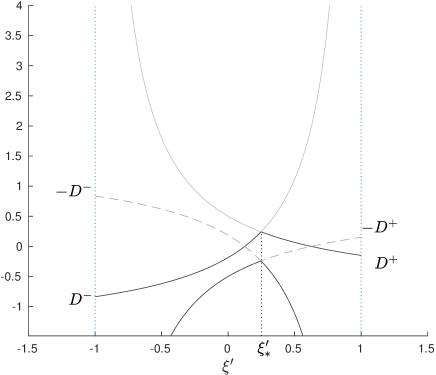
Figure 7: Illustration of relation (35). Here $D^{\pm}$ denote $d_{\rm nod}^{\pm}$ regarded as functions of $\xi,\xi^{\prime}$.

Thus we conclude that the maximal value of $\delta_{\rm ext}$ over ${\cal D}_{3}$ is

$$u^{\>e}_{\rm ext}(q,e)=\left\{\begin{array}[]{ll}p-p^{\prime}&\mbox{ if }p^{\prime}\leq p\cr m_{\rm ext}(q,e)&\mbox{ if }p^{\prime}>p\cr\end{array}\right.,$$ (36)

for some $m_{\rm ext}<(p-p^{\prime})/2<0$. Therefore, for each $(q,e)\in{\cal D}_{4}$ we obtain

$$\max\{\max_{(\omega,\omega^{\prime})\in{\cal D}_{3}}\delta_{\rm int},\max_{(\omega,\omega^{\prime})\in{\cal D}_{3}}\delta_{\rm ext}\}=|p^{\prime}-q(1+e)|.$$ (37)

  

  

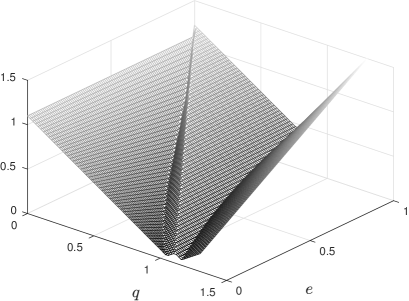
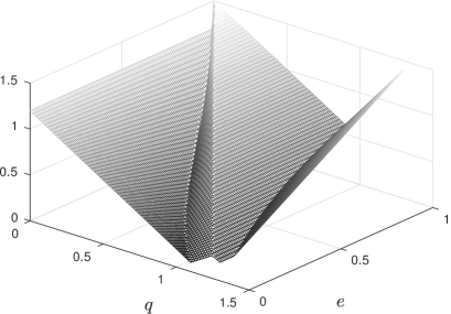
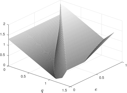
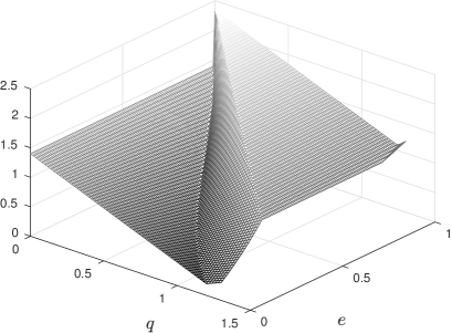
Figure 8: Graphic of $(q,e)\mapsto\max_{(\omega,\omega^{\prime})\in{\cal D}_{3}}\delta_{\rm nod}(q,e)$ for $e^{\prime}=0.1$ (top left), $e^{\prime}=0.2$ (top right), $e^{\prime}=0.3$ (bottom left), $e^{\prime}=0.4$ (bottom right). Here we set $q^{\prime}=1$.

Finally, we consider the function $\delta_{\rm link}$ and examine $\delta_{\rm link}^{(i)}$ and $\delta_{\rm link}^{(ii)}$ separately. By Lemma 1, both $-d_{\rm nod}^{+}$ and $d_{\rm nod}^{-}$ are non-decreasing functions of $\omega$ and non-increasing functions of $\omega^{\prime}$, therefore also $\delta_{\rm link}^{(i)}$ is. For each fixed value of $(q,e)$, the maximal value of $\delta_{\rm link}^{(i)}$ over ${\cal D}_{3}$ is attained for $\omega={\pi}/{2}$, $\omega^{\prime}=0$ and is

$$\min\{q(1+e)-q^{\prime},Q^{\prime}-q(1+e)\}.$$

In a similar way we prove that, for each fixed value of $(q,e)$, the maximal value of $\delta_{\rm link}^{(ii)}$ over ${\cal D}_{3}$ is attained for $\omega=0$, $\omega^{\prime}=\pi$ and is

$$\min\Bigl{\{}Q^{\prime}-q,\frac{q(1+e)}{1-e}-q^{\prime}\Bigr{\}}.$$

Therefore the maximal value of $\delta_{\rm link}$ over ${\cal D}_{3}$ is attained by $\delta_{\rm link}^{(ii)}$ and corresponds to

$$u^{\>e}_{\rm link}(q,e)=\ \min\Bigl{\{}\frac{q(1+e)}{1-e}-q^{\prime},Q^{\prime}-q\Bigr{\}}.$$

We conclude the proof of relation (30) using (3), (37) and the optimal bound

$$\delta_{\rm link}(q,e,\omega,\omega)\leq u^{\>e}_{\rm link}(q,e).$$

∎

In Figure 8 we show the graphic of $\max_{(\omega,\omega^{\prime})\in{\cal D}_{3}}\delta_{\rm nod}(q,e)$ for different values of $e^{\prime}$, with $q^{\prime}=1$.

Proposition 4.

The zero level curves of $\ell^{\>e}_{\rm int},\ell^{\>e}_{\rm ext},p^{\prime}-q(1+e)$ divide the plane $(q,e)$ into regions where different linking configurations are allowed.

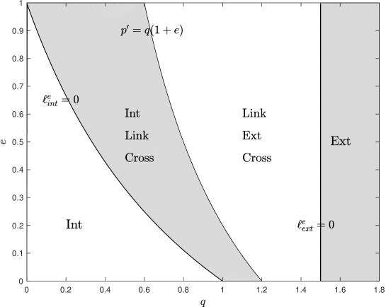
Figure 9: Regions with different linking configurations in the plane $(q,e)$ for $q^{\prime}=1$ and $e^{\prime}=0.2$.

Proof.

By Lemma 5, given $(q,e)\in{\cal D}_{4}$, we have internal nodes for each $(\omega,\omega^{\prime})\in{\cal D}_{3}$ if and only if $\ell^{\>e}_{\rm int}(q,e)>0$, therefore the region where only internal nodes are possible is delimited on the right by the curve $\ell^{\>e}_{\rm int}(q,e)=0$. In a similar way, the region with only external nodes is delimited on the left by $\ell^{\>e}_{\rm ext}(q,e)=0$.

Moreover, given $(q,e)$, we have internal nodes (resp. external nodes) for some choice of $(\omega,\omega^{\prime})$ if and only if $u^{\>e}_{\rm int}(q,e)>0$ (resp. $u^{\>e}_{\rm ext}(q,e)>0$). From relations (34), (36) we obtain that both the curves $u^{\>e}_{\rm int}(q,e)=0$ and $u^{\>e}_{\rm ext}(q,e)=0$ correspond to $p^{\prime}-q(1+e)=0$. Therefore, we can not have both the cases of internal and external nodes with the same value of $(q,e)$.

In a similar way, given $(q,e)$, we have linked orbits for some choice of $(\omega,\omega^{\prime})$ if and only if $u^{\>e}_{\rm link}(q,e)>0$. We note that the curve

$$u^{\>e}_{\rm link}(q,e)=0,$$

delimiting the region where linked orbits are possible, coincides with the curve

$$\{\ell^{\>e}_{\rm int}(q,e)=0\}\cup\{\ell^{\>e}_{\rm ext}(q,e)=0\}.$$

∎

Remark 3.

There can not exist $(q,e)\in{\cal D}_{4}$ such that we have linked orbits for each $(\omega,\omega^{\prime})\in{\cal D}_{3}$.

Proof.

If there exists $(q,e)\in{\cal D}_{4}$ such that $\delta_{\rm link}(q,e,\omega,\omega^{\prime})>0$ for each $(\omega,\omega^{\prime})\in{\cal D}_{3}$, then in particular $u^{\>e}_{\rm link}(q,e)>0$, and this corresponds to $\ell^{\>e}_{\rm int},\ell^{\>e}_{\rm ext}<0$ at $(q,e)$, so that, by ii) of Lemma 5, there exists $(\omega,\omega^{\prime})$ corresponding to a crossing configuration, that yields a contradiction.

∎

In Figure 9 we show the possible linking configurations for $q^{\prime}=1$ and $e^{\prime}=0.2$.

Next we present optimal bounds for $\delta_{\rm nod}$ as functions of $(q,\omega^{\prime})$. To this aim, we let $\omega$ vary in $[0,\pi]$ and $\omega^{\prime}$ in $[0,\pi/2]$, which is a different choice with respect to (2), however it also allows us to get all the possible values of $\delta_{\rm nod}$.

Proposition 5.

Let ${\cal D}_{5}=\{(e,\omega):0\leq e\leq 1,0\leq\omega\leq\pi\}$, ${\cal D}_{6}=\{(q,\omega^{\prime}):0<q\leq q_{\rm max},0\leq\omega^{\prime}\leq\pi/2\}$. For each choice of $(q,\omega^{\prime})\in{\cal D}_{6}$ we have

$$\displaystyle\min_{(e,\omega)\in{\cal D}_{5}}\delta_{\rm nod}=\max\bigl{\{}0,\ell^{\omega^{\prime}}_{\rm ext}\bigr{\}},$$ (38)

$$\displaystyle\max_{(e,\omega)\in{\cal D}_{5}}\delta_{\rm nod}=\max\Bigl{\{}u^{\omega^{\prime}}_{\rm link},u^{\omega^{\prime}}_{\rm ext}\Bigr{\}},$$ (39)

where

$$\ell^{\omega^{\prime}}_{\rm ext}(q,\omega^{\prime})=q-\frac{p^{\prime}}{1-e^{\prime}\cos\omega^{\prime}},$$

$$u^{\omega^{\prime}}_{\rm link}(q,\omega^{\prime})=\frac{p^{\prime}}{1-e^{\prime}\cos\omega^{\prime}}-q,$$

and

$$u^{\omega^{\prime}}_{\rm ext}(q,\omega^{\prime})=\frac{2q}{1+\cos\omega_{*}}-\frac{p^{\prime}}{1+e^{\prime}\cos\omega^{\prime}},$$

with

$$\cos\omega_{*}=\frac{p^{\prime}e^{\prime}\cos\omega^{\prime}}{\sqrt{q^{2}(1-e^{\prime 2}\cos^{2}\omega^{\prime})^{2}+(p^{\prime}e^{\prime}\cos\omega^{\prime})^{2}}+q(1-e^{\prime 2}\cos^{2}\omega^{\prime})}.$$

We prove some preliminary facts.

Lemma 7.

The following properties hold:

• for each $(q,\omega^{\prime})\in{\cal D}_{6}$ and $(e,\omega)\in{\cal D}_{5}$ we have

  $$\inf_{(e,\omega)\in{\cal D}_{5}}\delta_{\rm int}(q,e,\omega,\omega^{\prime})=-\infty,$$ (40)

  $$\delta_{\rm ext}(q,e,\omega,\omega^{\prime})\geq\delta_{\rm ext}(q,0,\omega,\omega^{\prime})=\ell^{\omega^{\prime}}_{\rm ext}(q,\omega^{\prime}).$$ (41)

• If $(q,\omega^{\prime})$ is such that $\ell^{\omega^{\prime}}_{\rm ext}(q,\omega^{\prime})\leq 0$, then there exists $(e,\omega)\in{\cal D}_{5}$ such that $d_{\rm nod}^{+}d_{\rm nod}^{-}=0$.

Proof.

Setting $e_{k}=1-\frac{1}{k},\omega_{k}=\frac{1}{k}$, $k\in\mathbb{N}$, we have

$$\lim_{k\to\infty}\delta_{\rm int}(q,e_{k},\omega_{k},\omega^{\prime})=-\infty$$

for each $(q,\omega^{\prime})\in{\cal D}_{6}$. We prove the bound (41) by observing that for each $(q,\omega^{\prime})\in{\cal D}_{6}$ and $(e,\omega)\in{\cal D}_{5}$ we have

$$\begin{split}\delta_{\rm ext}&\geq\min\biggl{\{}\min_{(e,\omega)\in{\cal D}_{5}}r_{\scaleto{+}{5pt}}-r_{\scaleto{+}{5pt}}^{\prime},\min_{(e,\omega)\in{\cal D}_{5}}r_{\scaleto{-}{5pt}}-r_{\scaleto{-}{5pt}}^{\prime}\biggr{\}}\cr&=\min\{r_{\scaleto{+}{5pt}}|_{e=0}-r_{\scaleto{+}{5pt}}^{\prime},r_{\scaleto{-}{5pt}}|_{e=0}-r_{\scaleto{-}{5pt}}^{\prime}\}=q-\frac{p^{\prime}}{1-e^{\prime}\cos\omega^{\prime}},\cr\end{split}$$

where the last equality holds because $\omega^{\prime}\in[0,\pi/2]$.

To prove $ii)$ we observe that by Lemma 1, for each $(q,\omega^{\prime})\in{\cal D}_{6}$, the maximal value of $\delta_{\rm ext}$ is attained at $e=1$, whatever the value of $\omega$. By the same lemma, $-d_{\rm nod}^{+}$ is a non-decreasing function of $\omega$, while $-d_{\rm nod}^{-}$ is non-increasing, whatever the value of $e$. Since

$$\bigl{.}\lim_{\omega\to 0^{+}}d_{\rm nod}^{+}\bigr{|}_{e=1}=\frac{p^{\prime}}{1+\xi^{\prime}}-q,\qquad\bigl{.}\lim_{\omega\to\pi^{-}}d_{\rm nod}^{+}\bigr{|}_{e=1}=-\infty,$$

and

$$\bigl{.}\lim_{\omega\to 0^{+}}d_{\rm nod}^{-}\bigr{|}_{e=1}=-\infty,\qquad\bigl{.}\lim_{\omega\to\pi^{-}}d_{\rm nod}^{-}\bigr{|}_{e=1}=\frac{p^{\prime}}{1-\xi^{\prime}}-q,$$

there is always a value $\omega_{*}$ of $\omega\in[0,\pi]$ such that

$$\bigl{.}d_{\rm nod}^{+}\bigr{|}_{e=1,\omega=\omega_{*}}=\bigl{.}d_{\rm nod}^{-}\bigr{|}_{e=1,\omega=\omega_{*}},$$ (42)

and this is given by relation

$$\cos\omega_{*}=\frac{p^{\prime}e^{\prime}\cos\omega^{\prime}}{\sqrt{q^{2}(1-e^{\prime 2}\cos^{2}\omega^{\prime})^{2}+(p^{\prime}e^{\prime}\cos\omega^{\prime})^{2}}+q(1-e^{\prime 2}\cos^{2}\omega^{\prime})}.$$ (43)

We conclude that the maximal value of $\delta_{\rm ext}$ over ${\cal D}_{5}$ is given by

$$u^{\omega^{\prime}}_{\rm ext}(q,\omega^{\prime})=\frac{2q}{1+\cos\omega_{*}}-\frac{p^{\prime}}{1+e^{\prime}\cos\omega^{\prime}}=\frac{2q}{1-\cos\omega_{*}}-\frac{p^{\prime}}{1-e^{\prime}\cos\omega^{\prime}}.$$ (44)

If $u^{\omega^{\prime}}_{\rm ext}(q,\omega^{\prime})\geq 0$, then there exists $(e,\omega)\in{\cal D}_{5}$ corresponding to a crossing configuration because we are assuming $\ell^{\omega^{\prime}}_{\rm ext}(q,\omega^{\prime})\leq 0$. On the other hand, if $u^{\omega^{\prime}}_{\rm ext}(q,\omega^{\prime})<0$ we have $\delta_{\rm ext}(q,e,\omega,\omega^{\prime})<0$ for each $(e,\omega)\in{\cal D}_{5}$. However, this assumption yields a contradiction, in fact one of the following cases holds:

• $\delta_{\rm int}(q,e,\omega,\omega^{\prime})>0$ for some $(e,\omega)\in{\cal D}_{5}$;

• $\delta_{\rm int}(q,e,\omega,\omega^{\prime})<0$ for each $(e,\omega)\in{\cal D}_{5}$, that is,

  $$u^{\omega^{\prime}}_{\rm int}(q,\omega^{\prime})=\max_{(e,\omega)\in{\cal D}_{5}}\delta_{\rm int}(q,\omega^{\prime})<0.$$

If a) holds, then by relation (40) and the continuity of $\delta_{\rm int}$ there exists $(e,\omega)\in{\cal D}_{5}$ yielding a crossing configuration. Instead, if b) holds, from $u^{\omega^{\prime}}_{\rm int}<0$ and $u^{\omega^{\prime}}_{\rm ext}<0$ we obtain that $d_{\rm nod}^{+}d_{\rm nod}^{-}<0$ at $(q,\omega^{\prime})$ for each $(e,\omega)\in{\cal D}_{5}$, that is, for the considered pair $(q,\omega^{\prime})$ we always have linked orbits. However, this contradicts relation (42).

∎

We continue the proof of Proposition 5.

Proof.

Lower bound: (38) follows from Lemma 7.

Upper bound: By Lemma 1 we obtain

$$\delta_{\rm int}(q,e,\omega,\omega^{\prime})\leq\delta_{\rm int}(q,0,\omega,\omega^{\prime})=\min\Bigl{\{}\frac{p^{\prime}}{1+e^{\prime}\cos\omega^{\prime}}-q,\frac{p^{\prime}}{1-e^{\prime}\cos\omega^{\prime}}-q\Bigr{\}}$$

for each $(q,\omega^{\prime})\in{\cal D}_{6}$, and each $(e,\omega)\in{\cal D}_{5}$. We conclude that the maximal value of $\delta_{\rm int}$ over ${\cal D}_{5}$ is

$$u^{\omega^{\prime}}_{\rm int}(q,\omega^{\prime})=\frac{p^{\prime}}{1+e^{\prime}\cos\omega^{\prime}}-q.$$ (45)

The maximal value of $\delta_{\rm ext}$ over ${\cal D}_{5}$ has been computed in Lemma 7 and is given in (44).

  

  

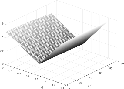
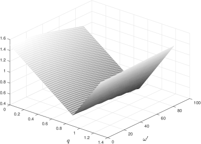
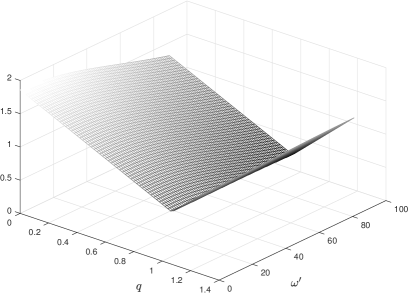
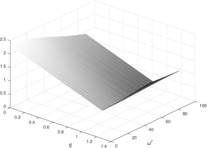
Figure 10: Graphic of $(q,\omega^{\prime})\mapsto\max_{(e,\omega)\in{\cal D}_{5}}\delta_{\rm nod}(q,\omega^{\prime})$ for $e^{\prime}=0.1$ (top left), $e^{\prime}=0.2$ (top right), $e^{\prime}=0.3$ (bottom left), $e^{\prime}=0.4$ (bottom right). Here we set $q^{\prime}=1$.

By Lemma 1, for each $(q,\omega^{\prime})\in{\cal D}_{6}$ the maximal value of $\delta_{\rm link}^{(i)}$ is attained at $\omega=\pi$ and the maximal value of $\delta_{\rm link}^{(ii)}$ is attained at $\omega=0$. We note that

$$\begin{split}\delta_{\rm link}^{(i)}|_{\omega=\pi}&=\min\Bigl{\{}\frac{q(1+e)}{1-e}-\frac{p^{\prime}}{1+e^{\prime}\cos\omega^{\prime}},\frac{p^{\prime}}{1-e^{\prime}\cos\omega^{\prime}}-q\Bigr{\}}\cr&\geq\min\Bigl{\{}\frac{p^{\prime}}{1+e^{\prime}\cos\omega^{\prime}}-q,\frac{q(1+e)}{1-e}-\frac{p^{\prime}}{1-e^{\prime}\cos\omega^{\prime}}\Bigr{\}}=\delta_{\rm link}^{(ii)}|_{\omega=0}\end{split}$$

for each $e\in[0,1]$. Therefore the maximal value of $\delta_{\rm link}$ over ${\cal D}_{5}$ is obtained by $\delta_{\rm link}^{(i)}$. By Lemma 1, $-d_{\rm nod}^{+}|_{\omega=\pi}$ is non-decreasing with $e$, while $d_{\rm nod}^{-}|_{\omega=\pi}$ is constant. Since

$$\lim_{e\to 1^{-}}-d_{\rm nod}^{+}|_{\omega=0}=+\infty$$

the maximal value of $\delta_{\rm link}$ over ${\cal D}_{5}$ is given by

$$u^{\omega^{\prime}}_{\rm link}(q,\omega^{\prime})=d_{\rm nod}^{-}|_{\omega=\pi}=\frac{p^{\prime}}{1-e^{\prime}\cos\omega^{\prime}}-q.$$ (46)

Finally, we note that $u^{\omega^{\prime}}_{\rm int}\leq u^{\omega^{\prime}}_{\rm link}$, therefore

$$\max_{(e,\omega)\in{\cal D}_{5}}\delta_{\rm nod}=\max\{u^{\omega^{\prime}}_{\rm int},u^{\omega^{\prime}}_{\rm link},u^{\omega^{\prime}}_{\rm ext}\}=\max\{u^{\omega^{\prime}}_{\rm link},u^{\omega^{\prime}}_{\rm ext}\}.$$

∎

In Figure 10 we show the graphic of $\max_{(e,\omega)\in{\cal D}_{5}}\delta_{\rm nod}(q,\omega^{\prime})$ for different values of $e^{\prime}$, with $q^{\prime}=1$. Using Remark 1 we can extend by symmetry the graphic of $\max_{(e,\omega)\in{\cal D}_{5}}\delta_{\rm nod}(q,\omega^{\prime})$ to the set $(0,q_{\rm max}]\times[0,2\pi)$.

Proposition 6.

The zero level curves of $\ell^{\omega^{\prime}}_{\rm ext},u^{\omega^{\prime}}_{\rm int},u^{\omega^{\prime}}_{\rm ext}$ divide the plane $(q,\omega^{\prime})$ into regions where different linking configurations are allowed. Moreover, the curve $u^{\omega^{\prime}}_{\rm ext}=0$ corresponds to the straight line $q=p^{\prime}/2$.

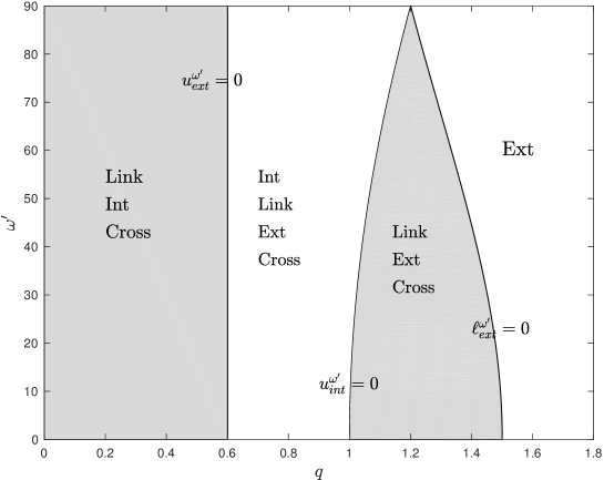
Figure 11: Regions with different linking configurations in the plane $(q,\omega^{\prime})$ for $q^{\prime}=1$ and $e^{\prime}=0.2$.

Proof.

By relation (40), given $(q,\omega^{\prime})\in{\cal D}_{6}$, we can not have internal nodes for each $(e,\omega)\in{\cal D}_{5}$. Moreover, we have only external nodes if and only if $\ell^{\omega^{\prime}}_{\rm ext}(q,\omega^{\prime})>0$, i.e. for $q>p^{\prime}/(1-e^{\prime}\cos\omega^{\prime})$. On the other hand, we have internal nodes for some choice of $(e,\omega)$ if and only if $u^{\omega^{\prime}}_{\rm int}(q,\omega^{\prime})>0$, i.e. for $q<p^{\prime}/(1+e^{\prime}\cos\omega^{\prime})$. Moreover, we have external nodes (resp. linked orbits) for some choice of $(e,\omega)$ if and only if $u^{\omega^{\prime}}_{\rm ext}(q,\omega^{\prime})>0$ (resp. $u^{\omega^{\prime}}_{\rm link}(q,\omega^{\prime})>0$).

We describe the shape of the curve $u^{\omega^{\prime}}_{\rm ext}(q,\omega^{\prime})=0$.

Eliminating $\cos\omega_{*}$ from equations

$$\frac{p^{\prime}}{1+e^{\prime}\cos\omega^{\prime}}-\frac{2q}{1+\cos\omega_{*}}=\frac{p^{\prime}}{1-e^{\prime}\cos\omega^{\prime}}-\frac{2q}{1-\cos\omega_{*}}=0$$

we obtain

$$q=\frac{p^{\prime}}{2}.$$ (47)

Vice versa, substituting $q=p^{\prime}/2$ into (43) we obtain

$$\cos\omega_{*}=e^{\prime}\cos\omega^{\prime},$$

so that $u^{\omega^{\prime}}_{\rm ext}(q,\omega^{\prime})=0$ for each $\omega^{\prime}\in[0,\pi/2]$. Therefore the curve $u^{\omega^{\prime}}_{\rm ext}=0$ is the straight line defined by (47).

∎

Remark 4.

There can not exist $(q,\omega^{\prime})\in{\cal D}_{6}$ such that we have linked orbits for each $(e,\omega)\in{\cal D}_{5}$.

Proof.

If $\delta_{\rm link}(q,e,\omega,\omega^{\prime})>0$ for each $(e,\omega)\in{\cal D}_{5}$ then in particular $u^{\omega^{\prime}}_{\rm link}(q,\omega^{\prime})>0$ and this corresponds to $\ell^{\omega^{\prime}}_{\rm ext}(q,\omega^{\prime})<0$ because $u^{\omega^{\prime}}_{\rm link}=-\ell^{\omega^{\prime}}_{\rm ext}$ . Therefore, by ii) of Lemma 7, there exists $(e,\omega)$ corresponding to a crossing configuration, that yields a contradiction.

∎

In Figure 11 we show the possible linking configurations for $q^{\prime}=1$ and $e^{\prime}=0.2$.

3.2 Bounds for $\delta_{\rm nod}$ when $e^{\prime}=0$

In this section we consider the particular case $e^{\prime}=0$, where ${\cal A}^{\prime}$ is circular. We recall some results proved in [5] concerning the orbit distance $d_{\rm min}$, that is the distance between the sets ${\cal A}$ and ${\cal A}^{\prime}$, and compare them with the corresponding results for the nodal distance $\delta_{\rm nod}$, that can be obtained by setting $e^{\prime}=0$ in the statements of Propositions 1, 3, 5.

Assume $q^{\prime}>0$ is given and let $e^{\prime}=0$. The following proposition, proved in [5], gives optimal bounds for $d_{\rm min}$ as functions of $(q,\omega)$.

Proposition 7.

Set ${\cal D}_{1}^{\prime}=\{(e,I):0\leq e\leq 1,0\leq I\leq\pi/2\}$ and ${\cal D}_{2}=\{(q,\omega):0<q\leq q_{\rm max},0\leq\omega\leq\pi/2\}$. For each choice of $(q,\omega)\in{\cal D}_{2}$ we have

$$\begin{array}[]{l}\displaystyle\min_{(e,I)\in{\cal D}_{1}^{\prime}}d_{\rm min}=\max\{0,q-q^{\prime}\},\\ \displaystyle\max_{(e,I)\in{\cal D}_{1}^{\prime}}d_{\rm min}=\max\{q^{\prime}-q,\delta_{\omega}(q,\omega)\},\\ \end{array}$$

where $\delta_{\omega}(q,\omega)$ is the distance between ${\cal A}^{\prime}$ and ${\cal A}$ with $e=1,I=\pi/2$:

$$\delta_{\omega}(q,\omega)=\sqrt{(\xi-q^{\prime}\sin\omega)^{2}+\Bigl{(}\frac{\xi^{2}-4q^{2}}{4q}+q^{\prime}\cos\omega\Bigr{)}^{2}}\,,$$ (48)

with $\xi=\xi(q,\omega)$ the unique real solution of

$$x^{3}+4q(q+\cos\omega)x-8q^{\prime}q^{2}\sin\omega=0.$$

We compare the above result with the following.

Proposition 8.

Set ${\cal D}^{\prime\prime}_{1}=\{e:0\leq e\leq 1\}$ and ${\cal D}_{2}=\{(q,\omega):0<q\leq q_{\rm max},0\leq\omega\leq{\pi}/{2}\}$. For each choice of $(q,\omega)\in{\cal D}_{2}$ we have

$$\displaystyle\min_{e\in{\cal D}_{1}^{\prime\prime}}\delta_{\rm nod}=\max\left\{0,q^{\prime}-\frac{2q}{1-\cos\omega},q-q^{\prime}\right\},$$ (49)

$$\displaystyle\max_{e\in{\cal D}_{1}^{\prime\prime}}\delta_{\rm nod}=\max\{q^{\prime}-q,\frac{2q}{1+\cos\omega}-q^{\prime}\}.$$ (50)

Proof.

We consider the statement of Proposition 1 for $e^{\prime}=0$, so that $Q^{\prime}=p^{\prime}=q^{\prime}$. By Lemma 1 we obtain

$$u^{\omega}_{\rm link}(q,\omega)\leq Q^{\prime}-\frac{q(1+\hat{e}_{*})}{1+\hat{e}_{*}\cos\omega}=p^{\prime}-\frac{q(1+\hat{e}_{*})}{1+\hat{e}_{*}\cos\omega}\leq p^{\prime}-q=u^{\omega}_{\rm int}(q,\omega).$$

Moreover, for $e^{\prime}=0$ we have $\hat{\xi}^{\prime}_{*}=0$, therefore

$$\frac{2q}{1-\cos\omega}-\frac{p^{\prime}}{1-\hat{\xi}_{*}^{\prime}}=\frac{2q}{1-\cos\omega}-q^{\prime},$$

so that

$$u^{\omega}_{\rm ext}(q,\omega)=\frac{2q}{1+\cos\omega}-q^{\prime},$$

and (4), (5) reduce to (49), (50).

∎

     

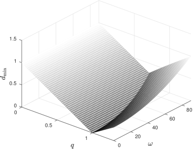
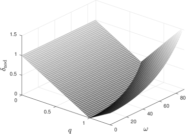
Figure 12: Left: $\max_{(e,I)\in{\cal D}_{1}^{\prime}}d_{\rm min}(q,\omega)$. Right: $\max_{e\in{\cal D}_{1}^{\prime\prime}}\delta_{\rm nod}(q,\omega)$.

In Figure 12, for $q^{\prime}=1$, we show the graphics of $\max_{(e,I)\in{\cal D}_{1}^{\prime}}d_{\rm min}(q,\omega)$ on the left, and of $\max_{e\in{\cal D}_{1}^{\prime\prime}}\delta_{\rm nod}(q,\omega)$ on the right.

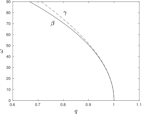
Figure 13: Comparison between the curves $\gamma$ and $\beta$.

In [5] the authors introduced the equation of a curve, denoted by $\gamma$, which separates the region in the plane $(q,\omega)$ where the trajectories maximizing $d_{\rm min}$ over ${\cal D}_{1}^{\prime}$ have $e=0$, from the region where such trajectories have $e=1$, that is, $\gamma$ is the set of points $(q,\omega)$ where $q^{\prime}-q$ and $\delta_{\omega}(q,\omega)$, defined in (48), assume the same values. This equation is

$$\begin{split}&2q^{4}+2q^{\prime}(-5+7y)q^{3}-2q^{\prime 2}(3y+22)(y-1)q^{2}+\cr&+q^{\prime 3}(y^{3}+13y^{2}+9y-27)q-2q^{\prime 4}y^{3}=0,\cr\end{split}$$ (51)

with $y=\cos\omega$. The analogous equation for $\delta_{\rm nod}$ is

$$qy+3q-2q^{\prime}y-2q^{\prime}=0,$$ (52)

that is easily obtained by equating $q^{\prime}-q$ with $\frac{2q}{1+\cos\omega}-q^{\prime}$. We denote by $\beta$ the curve defined by (52). In Figure 13 we plot both curves for comparison.

We also recall the following result (see [5]), stating optimal bounds for the orbit distance $d_{\rm min}$ as functions of $(q,e)$.

     

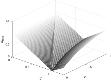
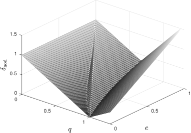
Figure 14: Left: $\max_{(I,\omega)\in{\cal D}_{3}^{\prime}}d_{\rm min}(q,e)$. Right: $\max_{\omega\in{\cal D}_{3}^{\prime\prime}}\delta_{\rm nod}(q,e)$.

Proposition 9.

Set ${\cal D}_{3}^{\prime}=\{(I,\omega):0\leq I\leq\pi/2,0\leq\omega\leq\pi/2\}$ and ${\cal D}_{4}=\{(q,e):0<q\leq q_{\rm max},0\leq e\leq 1\}$. For each choice of $(q,e)\in{\cal D}_{4}$ we have

$$\begin{array}[]{l}\displaystyle\min_{(I,\omega)\in{\cal D}_{3}^{\prime}}d_{\rm min}=\max\{0,q^{\prime}-Q,q-q^{\prime}\},\\ \displaystyle\max_{(I,\omega)\in{\cal D}_{3}^{\prime}}d_{\rm min}=\max\{\min\{q^{\prime}-q,Q-q^{\prime}\},\delta_{e}(q,e)\},\\ \end{array}$$

where $Q=q(1+e)/(1-e)$ is the (possibly infinite) apocenter distance and $\delta_{e}(q,e)$ is the distance between ${\cal A}^{\prime}$ and ${\cal A}$ with $I=\pi/2,\omega=\pi/2$:

$$\delta_{e}(q,e)=\sqrt{(\xi-q^{\prime})^{2}+\biggl{(}\frac{\xi^{2}-q^{2}(1+e)^{2}}{qe(1+e)+\sqrt{(1+e)(q^{2}-\xi^{2}(1-e))}}\biggr{)}^{2}}$$

where $\xi=\xi(q,e)$ is the unique real positive solution of

$$\begin{split}&e^{4}x^{4}+2q^{\prime}e^{2}(1-e^{2})x^{3}+(1+e)^{2}(q^{\prime 2}(1-e)^{2}+q^{2}e^{2})x^{2}\\ -\>&2q^{\prime}q^{2}e^{2}(1+e)^{2}x-q^{\prime 2}q^{2}(1-e^{2})(1+e)^{2}=0.\\ \end{split}$$

We compare the above result with the following.

Proposition 10.

Set ${\cal D}_{3}^{\prime\prime}=\{\omega:0\leq\omega\leq\pi/2\}$ and ${\cal D}_{4}=\{(q,e):0<q\leq q_{\rm max},0\leq e\leq 1\}$. For each choice of $(q,e)\in{\cal D}_{4}$ we have

$$\left\{\begin{array}[]{l}\displaystyle\min_{\omega\in{\cal D}_{3}^{\prime\prime}}\delta_{\rm nod}=\max\{0,q^{\prime}-Q,q-q^{\prime}\}\\ \displaystyle\max_{\omega\in{\cal D}_{3}^{\prime\prime}}\delta_{\rm nod}=\max\{\min\{q^{\prime}-q,Q-q^{\prime}\},|q^{\prime}-q(1+e)|\}.\\ \end{array}\right.$$ (53)

Proof.

The result follows immediately by setting $e^{\prime}=0$ in relations (29), (30).

∎

In Figure 14, for $q^{\prime}=1$, we show the graphics of $\max_{(I,\omega)\in{\cal D}_{3}^{\prime}}d_{\rm min}(q,e)$ on the left, and of $\max_{\omega\in{\cal D}_{3}^{\prime\prime}}\delta_{\rm nod}(q,e)$ on the right.

4 Applications to the discovery of near-Earth asteroids

In Figure 15 we show the distribution of the known population of near-Earth asteroids with absolute magnitude $H>22$ (faint NEAs) in the plane $(q,\omega)$. We have used the database of NEODyS (https://newton.spacedys.com/neodys) to the date of July 23, 2019. On the left of the curve $\ell^{\omega}_{\rm int}=0$, computed for $q^{\prime}=1$ au and $e^{\prime}=0$ and prolonged by symmetry, we can have only internal nodes (see also Figure 6), therefore asteroids with those values of $(q,\omega)$ are difficult to be observed because they are always on the side of the Sun. This explains why this region appears depopulated. On the other hand, we can see that several asteroids are concentrated in a neighborhood of the curve $\beta$, defined by equation (52) and prolonged by symmetry, which represents the set of pairs $(q,\omega)$ where the value of $\delta_{\rm nod}$ can not be too large, whatever the value of $e$. In [5] the concentration of faint NEAs along the curve $\gamma$ defined by equation (51) had already been noticed and explained by the same geometrical argument employing the orbit distance $d_{\rm min}$ instead of $\delta_{\rm nod}$. Here we observe that the curve $\beta$ is close to $\gamma$ (see Figure 13), but it has a much simpler expression, therefore it can be easily used for a quick computation.

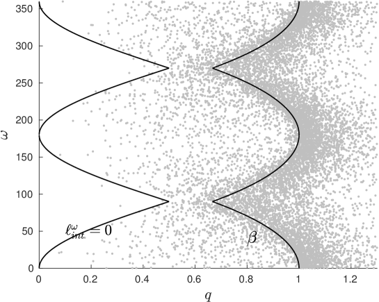
Figure 15: Orbital distribution of the known NEAs in the plane $(q,\omega)$. The gray dots correspond to faint asteroids ($H>22$).

5 Comparison with the orbit distance $d_{\rm min}$

In this section we discuss the analogies and the differences between the upper bounds found for $\delta_{\rm nod}$ in Propositions 1, 3, 5 and similar upper bounds for $d_{\rm min}$, computed by numerical methods.

In the mutual reference frame the coordinates of a point of ${\cal A}$ and another of ${\cal A}^{\prime}$ are given by

$$\left\{\begin{array}[]{l}x=r\cos(f+\omega)\cr y=r\sin(f+\omega)\cos I\cr z=r\sin(f+\omega)\sin I\cr\end{array}\right.\hskip 28.45274pt\left\{\begin{array}[]{l}x^{\prime}=r^{\prime}\cos(f^{\prime}+\omega^{\prime})\cr y^{\prime}=r^{\prime}\sin(f^{\prime}+\omega^{\prime})\cr z^{\prime}=0\end{array}\right.$$ (54)

where

$$r=\frac{q(1+e)}{1+e\cos f},\hskip 28.45274ptr^{\prime}=\frac{q^{\prime}(1+e^{\prime})}{1+e^{\prime}\cos f^{\prime}},$$

with $f,f^{\prime}\in[0,2\pi)$. Therefore, the squared distance between these two points is

$$d^{2} = (x-x^{\prime})^{2}+(y-y^{\prime})^{2}+z^{2}=$$

$$= r^{2}+r^{\prime 2}-2rr^{\prime}[\cos(f+\omega)\cos(f^{\prime}+\omega^{\prime})+\sin(f+\omega)\sin(f^{\prime}+\omega^{\prime})\cos I]=$$

$$= \frac{q^{2}(1+e)^{2}}{(1+e\cos f)^{2}}+\frac{q^{\prime 2}(1+e^{\prime})^{2}}{(1+e^{\prime}\cos f^{\prime})^{2}}-$$

$$- 2\frac{q(1+e)}{1+e\cos f}\frac{q^{\prime}(1+e^{\prime})}{1+e^{\prime}\cos f^{\prime}}[\cos(f+\omega)\cos(f^{\prime}+\omega^{\prime})+\sin(f+\omega)\sin(f^{\prime}+\omega^{\prime})\cos I]$$

From the expression above we see that we get all the possible values of the distance even if we restrict to the following ranges for $I,\omega,\omega^{\prime}$:

$$0\leq I\leq\pi/2,\qquad 0\leq\omega\leq\pi/2,\qquad 0\leq\omega^{\prime}<2\pi.$$

or

$$0\leq I\leq\pi/2,\qquad 0\leq\omega<2\pi,\qquad 0\leq\omega^{\prime}\leq\pi/2.$$

  

  

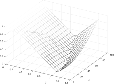
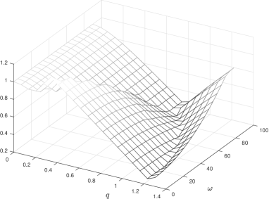
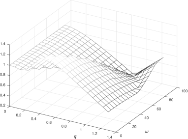
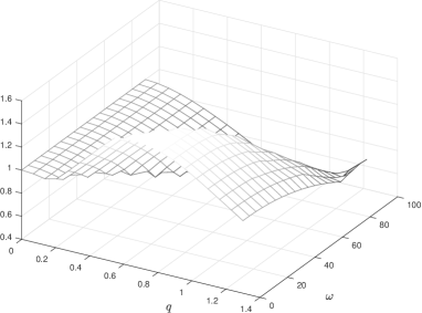
Figure 16: Graphic of $\max_{\widetilde{\cal D}_{1}}d_{\rm min}(q,\omega)$ for $e^{\prime}=0.1$ (top left), $e^{\prime}=0.2$ (top right), $e^{\prime}=0.3$ (bottom left), $e^{\prime}=0.4$ (bottom right). Here we set $q^{\prime}=1$.

In Figures 16, 17 we show, for different values of $e^{\prime}>0$, the graphics of $\max_{\widetilde{\cal D}_{1}}d_{\rm min}(q,\omega)$ and $\max_{\widetilde{\cal D}_{3}}d_{\rm min}(q,e)$, where

$$\begin{split}\widetilde{\cal D}_{1}&=\{(e,I,\omega^{\prime}):0\leq e\leq 1,\ 0\leq I\leq\pi/2,\ 0\leq\omega^{\prime}\leq 2\pi\},\cr\widetilde{\cal D}_{3}&=\{(I,\omega,\omega^{\prime}):0\leq I\leq\pi/2,\ 0<\omega\leq\pi/2,\ 0\leq\omega^{\prime}\leq 2\pi\}.\cr\end{split}$$

In both these cases we see that the graphics are similar to those in Figures 5, 8. In particular, the bulges appearing in the graphics of $\max_{{\cal D}_{1}}\delta_{\rm nod}$ when $e^{\prime}>0$ appear also in the graphics of $\max_{\widetilde{\cal D}_{1}}d_{\rm min}$.

  

  

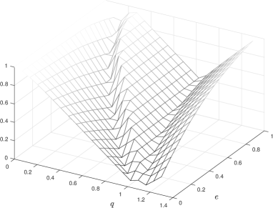
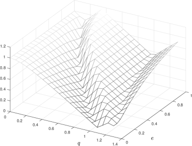
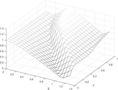
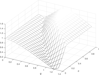
Figure 17: Graphic of $\max_{\widetilde{\cal D}_{3}}d_{\rm min}(q,e)$ for $e^{\prime}=0.1$ (top left), $e^{\prime}=0.2$ (top right), $e^{\prime}=0.3$ (bottom left), $e^{\prime}=0.4$ (bottom right). Here we set $q^{\prime}=1$.

  

  

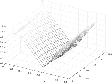
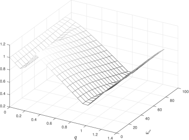
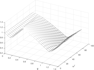
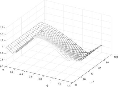
Figure 18: Graphic of $\max_{\widetilde{\cal D}_{5}}d_{\rm min}(q,\omega^{\prime})$ for $e^{\prime}=0.1$ (top left), $e^{\prime}=0.2$ (top right), $e^{\prime}=0.3$ (bottom left), $e^{\prime}=0.4$ (bottom right). Here we set $q^{\prime}=1$.

In Figure 18 we show, for the same values of $e^{\prime}$, the graphics of $\max_{\widetilde{\cal D}_{5}}d_{\rm min}(q,\omega^{\prime})$, where

$$\widetilde{\cal D}_{5}=\{(e,I,\omega):0\leq e\leq 1,\ 0\leq I\leq\pi/2,\ 0\leq\omega\leq 2\pi\}.$$

In this case the optimal bounds for $\delta_{\rm nod}$ displayed in Figure 10 has not the same features appearing here: in fact the bulges appearing in the graphics of $\max_{\widetilde{\cal D}_{5}}d_{\rm min}$ are not reproduced in the graphic of $\max_{{\cal D}_{5}}\delta_{\rm nod}$.

6 Conclusions

We have introduced optimal bounds for the nodal distance $\delta_{\rm nod}$ between a given bounded Keplerian trajectory ${\cal A}^{\prime}$ and another Keplerian trajectory ${\cal A}$, with a focus in common with the former, whose mutual orbital elements may vary. Besides being interesting in itself, this work aims at understanding how similar bounds can be stated and proved for the orbit distance $d_{\rm min}$. The conclusion is that the behavior of the upper bounds for $\delta_{\rm nod}$ given in Propositions 1, 3, as functions of $(q,\omega)$ and $(q,e)$, is similar to that for $d_{\rm min}$, obtained here by numerical computations. On the other hand, the upper bound for $\delta_{\rm nod}$ given in Proposition 5, as function of $(q,\omega^{\prime})$, is qualitatively different from that for $d_{\rm min}$. As a by-product of these results we have also found the equations of the curves dividing the planes with coordinates $(q,\omega)$, $(q,e)$, $(q,\omega^{\prime})$ into regions where different linking configurations are allowed.

7 Acknowledgements

Part of this work has been done during a visiting period of G.F. Gronchi at the Institut de mécanique céleste et de calcul des éphémérides (IMCCE), Observatoire de Paris. The same author also acknowledges the project MIUR-PRIN 20178CJA2B titled ”New frontiers of Celestial Mechanics: theory and applications”.

References

[1] Casanova, D., Tardioli, C. Lemaître, A.:
‘Space debris collision avoidance using a three-filter sequence’,
MNRAS 442, 3235-3242 (2014)
[2] Farnocchia, D., Chesley, S. R., Milani, A., Gronchi,
G. F., Chodas, P. W.: Orbits, Long-Term Prodictions, and Impact
Monitoring’, in Asteroids IV, Univ. of Arizona, Tucson (2016)
[3] Gronchi, G.F.: ‘On the stationary points of the
squared distance between two ellipses with a common focus’, SIAM
Journ. Sci. Comp. 24/1, 61-80 (2002)
[4] Gronchi, G.F.: ‘An algebraic method to compute the
critical points of the distance function between two Keplerian
orbits’, Cel. Mech. Dyn. Ast. 93/1, 297-332 (2005)
[5] Gronchi, G.F., Valsecchi, G.B.: ‘On the possible
values of the orbit distance between a near-Earth asteroid and the
Earth’, MNRAS 429/3, 2687-2699 (2013)
[6] Hoots, F. R., Crawford, L. L., Roehrich, R. L.: ‘An
Analytic Method to Determine Future Close Approaches Between
Satellites’, Cel. Mech. 33/2, 143-158 (1984)
[7] Kholshevnikov, K.V., Vassiliev, N.N.: ‘On linking
coefficient of two Keplerian orbits’, Cel. Mech. Dyn. Ast. 75/1, 67-74 (1999)
[8] Kholshevnikov, K.V., Vassiliev, N.N.: ‘On the
Distance Function Between Two Keplerian Elliptic Orbits’,
Cel. Mech. Dyn. Ast. 75/2, 75-83 (1999)
[9] Mikryukov, D.V., Baluev, R.V.: ‘A lower bound of the
distance between two elliptic orbits’, CMDA 131/6, First Online (2019)