Tarski’s Theorem, Supermodular Games, and the Complexity of Equilibria

Abstract

The use of monotonicity and Tarski’s theorem in existence proofs of equilibria is very widespread in economics, while Tarski’s theorem is also often used for similar purposes in the context of verification. However, there has been relatively little in the way of analysis of the complexity of finding the fixed points and equilibria guaranteed by this result. We study a computational formalism based on monotone functions on the $d$-dimensional grid with sides of length $N$, and their fixed points, as well as the closely connected subject of supermodular games and their equilibria. It is known that finding some (any) fixed point of a monotone function can be done in time $\log^{d}N$, and we show it requires at least $\log^{2}N$ function evaluations already on the 2-dimensional grid, even for randomized algorithms. We show that the general Tarski problem of finding some fixed point, when the monotone function is given succinctly (by a boolean circuit), is in the class $\mathsf{PLS}$ of problems solvable by local search and, rather surprisingly, also in the class $\mathsf{PPAD}$. Finding the greatest or least fixed point guaranteed by Tarski’s theorem, however, requires $d\cdot N$ steps, and is NP-hard in the white box model. For supermodular games, we show that finding an equilibrium in such games is essentially computationally equivalent to the Tarski problem, and finding the maximum or minimum equilibrium is similarly harder. Interestingly, two-player supermodular games where the strategy space of one player is one-dimensional can be solved in $O(\log N)$ steps. We also observe that computing (approximating) the value of Condon’s (Shapley’s) stochastic games reduces to the Tarski problem. An important open problem highlighted by this work is proving a $\Omega(\log^{d}N)$ lower bound for small fixed dimension $d\geq 3$; we discuss certain promising approaches.

1 Introduction

Equilibria are paramount in economics, because guaranteeing their existence in a particular strategic or market-like framework enables one to consider “What happens at equilibrium?” without further analysis. Equilibrium existence theorems are nontrivial to prove. The best known example is Nash’s theorem [18], whose proof in 1950, based on Brouwer’s fixed point theorem, transformed game theory, and inspired the Arrow-Debreu price equilibrium results [1], among many others. Decades later, complexity analysis of these theorems and corresponding solution concepts by computer scientists has created a fertile and powerful field of research [19].

Not all equilibrium theorems in economics, however, rely on Brouwer’s fixed point theorem for their proof (even though, in a specific sense made clear and proved in this paper, they could have…). Many of the exceptions ultimately rely on Tarski’s fixed point theorem [22], stating that all monotone functions on a complete lattice have a fixed point — and in fact a whole sublattice of fixed points with a largest and smallest element [23, 17, 24]. In contrast to the equilibrium theorems whose proof relies on Brouwer’s fixed point theorem, there has been relatively little complexity analysis of Tarski’s fixed point theorem and the equilibrium results it enables. (We discuss prior related work at the end of this introduction.)

Here we present several results in this direction. Let $[N]=\{1,\ldots,N\}$. To formulate the basic problem, we consider a monotone function $f$ on the $d$-dimensional grid $[N]^{d}$, that is, a function $f:[N]^{d}\mapsto[N]^{d}$ such that for all $x,y\in[N]^{d}$, $x\geq y$ implies $f(x)\geq f(y)$; in the black-box oracle model, we can query this function with specific vectors $x\in[N]^{d}$; in the white-box model we assume that the function is presented by a boolean circuit. Thus, $d$ and $N$ are the basic parameters to our model; it is useful to think of $d$ as the dimensionality of the problem, while $N$ is something akin to the inverse of the desired approximation $\epsilon$.

• Tarski’s theorem in the grid framework is easy to prove. Let $\bar{1}=(1,\ldots,1)$ denote the ($d$-dimensional) all-1 vector. Consider the sequence of grid points $\bar{1},f(\bar{1}),f(f(\bar{1})),\ldots,f^{i}(\bar{1}),\ldots$. From monotonicity of $f$, by induction on $i$ we get, for all $i\geq 0$, $f^{i}(\bar{1})\leq f^{i+1}(\bar{1})$. Unless a fixed point is arrived at, the sum of the coordinates must increase at each iteration. Therefore, after at most $dN$ iterations of $f$ applied to $\bar{1}$, a fixed point is found. In other words $f^{dN}(\bar{1})=f^{dN+1}(\bar{1})$.

• This immediately suggests an $O(dN)$ algorithm. But an $O(\log^{d}N)$ algorithm is also known: Consider the $(d-1)$-dimensional function obtained by fixing the “input value” in the $d$’th coordinate of the function $f$ with some value $r_{d}$ (initialize $r_{d}:=\lceil N/2\rceil$). Find a fixed point $z^{*}\in[N]^{d-1}$ of this $(d-1)$-dimensional monotone function $f(z,r_{d})$ (recursively). If the $d$th coordinate $f_{d}(z^{*},r_{d})$ of $f(z^{*},r_{d})$, is equal to $r_{d}$, then $(z^{*},r_{d})$ is a fixed point of the overall function $f$, and we are done. Otherwise, a binary search on the $d$’th coordinate is enabled: we need to look for a larger (smaller) value of $r_{d}$ if $f_{d}(z^{*},r_{d})>r_{d}$ (respectively, if $f_{d}(z^{*},r_{d})<r_{d}$). By an easy induction, this establishes the $O(\log^{d}N)$ upper bound ([5]).

• We conjecture that this algorithm is essentially optimal in the black box sense, for small fixed constant dimension $d$. In Theorem 4.1 we prove this result for the $d=2$ case. We provide a class of monotone functions that we call the herringbones: two monotonic paths, one starting from $\bar{1}$ and the other from $\bar{N}$, meeting at the fixed point, while all other points in the $N\times N$ grid are mapped diagonally: $f(x)=x+(-1,+1)$ or $x+(+1,-1)$, whichever of the points is closer to the monotonic path that contains the fixed point. We prove that any randomized algorithm needs to make $\Omega(\log^{2}N)$ queries (with high probability) to find the fixed point.

• Can this lower bound result be generalized to fixed $d\geq 3$? This is a key question left open by this paper. There are several obstacles to a proof establishing, e.g., a $\Omega(\log^{3}N)$ lower bound in the 3-dimensional case ($d=3$), and some possible ways for overcoming them. First, it is not easy to identify a suitable “herringbone-like” function in three or more dimensions — a monotone family of functions built around a path from $\bar{1}$ to $\bar{N}$. It nevertheless seems plausible that $\log^{d}N$ should still be (close to) a lower bound on any such algorithm (assuming of course that $N$ is sufficiently larger than $d$, so that the $dN$ algorithm does not violate the lower bound). We prove one encouraging result in this context: We give an alternative proof of the $d=2$ lower bound, in which we establish that any deterministic black-box algorithm for Tarski in two dimensions must solve a sequence of $\Omega(\log N)$ one-dimensional problems (Theorem 4.7), a result pointing to a possible induction on $d$ (recall that this is precisely the form of the $\log^{d}N$ algorithm).

• Tarski’s theorem further asserts that there is a greatest and a least fixed point, and these fixed points are especially useful in the economic applications of the result (see for example [17]). It is not hard to see, however, that finding these fixed points is NP-hard, and takes $\Omega(dN)$ time in the black box model (see Proposition 2.1).

• In terms of complexity classes, the problem Tarski is obviously in the class TFNP of total function (total search) problems. But where exactly? We show (Theorem 3.2) that it belongs in the class $\mathsf{PLS}$ of local optimum search problems.

• Surprisingly, Tarski is also in the class $P^{\mathsf{PPAD}}$ of problems reducible to a Brouwer fixed point problem (Theorem 3.3), and thus, by the known fact that the class $\mathsf{PPAD}$ is closed under polynomial time Turing reductions ([2]) it is in $\mathsf{PPAD}$ (Corollary 3.4). This result presents a heretofore unsuspected connection between two main sources of equilibrium results in economics.

• Supermodular games [23, 17, 24] — or games with strategic complementarities — comprise a large and important class of economic models, with complete lattices as strategy spaces, in which a player’s best response is a monotone function (or monotone correspondence) of the other player’s strategies. They always have pure Nash equilibria due to Tarski’s theorem. We show that finding an equilibrium for a supermodular game with (discrete) Euclidean grid strategy spaces is essentially computationally equivalent to the problem of finding a Tarski fixed point of a monotone map (Proposition 5.2 and Theorem 5.4). If there are two players and one of them has a one-dimensional strategy space, we show that a Nash equilibrium can be found in logarithmic time (in the size of the strategy spaces).

• Stochastic games [21, 4]. We show that the problems of computing the (irrational) value of Shapley’s discounted stochastic games to desired accuracy, and computing the exact value of Condon’s simple stochastic games (SSG), are both P-time reducible to the Tarski problem. The proofs employ known characterizations of the value of both Shapley’s stochastic games and Condon’s SSGs in terms of monotone fixed point equations, which can also be viewed as monotone “polynomially contracting” maps with a unique fixed point, and from properties of polynomially contracting maps, see [11].

Prior related work: in recent years a number of technical reports and papers by Dang, Qi, and Ye, have considered the complexity of computational problems related to Tarski’s theorem [5, 6, 7]. In particular, in [5] the authors provided the already-mentioned $\log^{d}N$ algorithm for computing a Tarski fixed point for a discrete map, $f:[N]^{d}\rightarrow[N]^{d}$, which is monotone under the coordinate-wise order. In [5] they also establish that determining the uniqueness of the fixed point of a monotone map under coordinate-wise order is coNP-hard, and that uniqueness under lexicographic order is also coNP-hard (already in one dimension). In [6] the authors studied another variant of the Tarski problem, namely computing another fixed point of a monotone function in an expanded domain where the smallest point is a fixed point; this variant is NP-hard (the claim in the paper that this problem is in $\mathsf{PPA}{}$ has been withdrawn by the authors [8]). In earlier work, Echenique [10], studied algorithms for computing all pure Nash equilibria in supermodular games (and games with strategic complementaries) whose strategy spaces are discrete grids. Of course computing all pure equilibria is harder than computing some pure equilibrium; indeed, we show that computing the least (or greatest) pure equilibrium of such a supermodular game is already NP-hard (Corollary 5.5). In earlier work Chang, Lyuu, and Ti [3] considered the complexity of Tarski’s fixed point theorem over a general finite lattice given via an oracle for its partial order (not given it explicitly) and given an oracle for the monotone function, and they observed that the total number of oracle queries required to find some fixed point in this model is linear in the number of elements of the lattice. They did not study monotone functions on euclidean grid lattices, and their results have no bearing on this setting.

2 Basics

A partial order $(L,\leq)$ is a complete lattice if every nonempty subset $S$ of $L$ has a least upper bound (or supremum or join, denoted $\sup S$ or $\lor S$) and a greatest lower bound (or infimum or meet, denoted $\inf S$ or $\land S$) in $L$. A function $f:L\rightarrow L$ is monotone if for all pairs of elements $x,y\in L$, $x\leq y$ implies $f(x)\leq f(y)$. A point $x\in L$ is a fixed point of $f$ if $f(x)=x$. Tarski’s theorem ([22]) states that the set $Fix(f)$ of fixed points of $f$ is a nonempty complete lattice under the same partial order $\leq$; in particular, $f$ has a greatest fixed point (GFP) and a least fixed point (LFP).

In this paper we will take as our underlying lattice $L$ a finite discrete Euclidean grid, which we fix for simplicity to be the integer grid $[N]^{d}$, for some positive integers $N,d$, where $[N]=\{1,\ldots,N\}$. Comparison of points is componentwise, i.e. $x\leq y$ if $x_{i}\leq y_{i}$ for all $i=1,\ldots,d$. We will also consider the corresponding continuous box, $[1,N]^{d}$ that includes all real points in the box. Both, the discrete and continuous box are clearly complete lattices.

Given a monotone function $f$ on the integer grid $[N]^{d}$, the problem is to compute a fixed point of $f$ (any point in $Fix(f)$). A generally harder problem is to compute specifically the LFP of $f$ or the GFP of $f$. We consider mostly the oracle model, in which the function $f$ is given by a black-box oracle, and the complexity of the algorithm is measured in terms of the number of queries to the oracle. Alternatively, we can consider also an explicit model in which $f$ is given explicitly by a polynomial-time algorithm (a polynomial-size Boolean circuit), and then the complexity of the algorithm is measured in the ordinary Turing model. Note that the number of bits needed to represent a point in the domain is $d\log N$, so polynomial time here means polynomial in $d$ and $n=\log N$. The number $N^{d}$ of points in the domain is exponential.

Tarski’s value iteration algorithm provides a simple way to compute the LFP of $f$: Starting from the lowest point of the lattice, which here is the all-1 vector $1$, apply repeatedly $f$. This generates a monotonically increasing sequence of points $1\leq f(1)\leq f^{2}(1)\leq\ldots$ until a fixed point is reached, which is the LFP of $f$. In every step of the sequence, at least one coordinate is strictly increased, therefore a fixed point is reached in at most $(N-1)d$ steps. In the worst case, the process may take that long, which is exponential in the bit size $d\log N$. Similarly, the GFP can be computed by applying repeatedly $f$ starting from the highest point of the lattice, i.e., from the all-$N$ point, until a fixed point is reached.

Another way to compute some fixed point of a monotone function $f$ (not necessarily the LFP or the GFP) is by a divide-and-conquer algorithm. In one dimension, we can use binary search: If the domain is the set $L(l,h)=\{x\in Z|l\leq x\leq h\}$ of integers between the lowest point $l$ and the highest point $h$, then compute the value of $f$ on the midpoint $m=(l+h)/2$. If $f(m)=m$ then $m$ is a fixed point; if $f(m)<m$ then recurse on the lower half $L(l,m)$, and if $f(m)>m$ then recurse on the upper half $L(m,h)$. The monotonicity of $f$ implies that $f$ maps the respective half interval into itself. Hence the algorithm correctly finds a fixed point in at most $\log N$ iterations, where $N$ is the number of points.

In the general $d$-dimensional case, suppose that the domain is the set of integer points in the box defined by the lowest point $l$ and the highest point $h$, i.e. $L(l,h)=\{x\in Z^{d}|l\leq x\leq h\}$. Consider the set of points with $d$-th coordinate equal to $m=(l+h)/2$; their first $d-1$ coordinates induce a $(d-1)$-dimensional lattice $L^{\prime}(l,h)=\{x\in Z^{d-1}|l_{i}\leq x_{i}\leq h_{i},i=1,\ldots d-1\}$. Define the function $g$ on $L^{\prime}(l,h)$ by letting $g(x)$ consist of the first $d-1$ components of $f(x,m)$. It is easy to see that $g$ is a monotone function on $L^{\prime}(l,h)$. Recursively, compute a fixed point $x^{*}$ of $g$. If $f_{d}(x^{*},m)=m$, then $(x^{*},m)$ is a fixed point of $f$ (this holds in particular if $l=h$). If $f_{d}(x^{*},m)>m$, then recurse on $L(f(x^{*},m),h)$. If $f_{d}(x^{*},m)<m$, then recurse on $L(l,f(x^{*},m))$. In either case, monotonicity implies that if the algorithm recurses, then $f$ maps the smaller box into itself and thus has a fixed point in it. An easy induction shows that the complexity of this algorithm is $O((\log N)^{d})$, ([5]).

Computing the least or the greatest fixed point is in general hard, even in one dimension, both in the oracle and in the explicit model.

Proposition 2.1.

Computing the LFP or the GFP of an explicitly given polynomial-time monotone function in one dimension is NP-hard. In the oracle model, the problem requires $\Omega(N)$ queries for a domain of size $N$.

Proof.

We prove the claim for the LFP; the GFP is similar. Reduction from Satisfiability. Given a Boolean formula $\phi$ in $n$ variables, let the domain $D=\{0,1,\ldots,2^{n}\}$, and define the function $f$ as follows. For $x\leq 2^{n}-1$, viewing $x$ as an $n$-bit binary number, it corresponds to an assignment to the $n$ variables of $\phi$; let $f(x)=x$ if the assignment $x$ satisfies $\phi$, and let $f(x)=x+1$ otherwise. Define $f(2^{n})=2^{n}$. Clearly $f$ is a monotone function and it can be computed in polynomial time. If $\phi$ is not satisfiable then the LFP of $f$ is $2^{n}$, while if $\phi$ is satisfiable then the LFP is not $2^{n}$.

For the oracle model, use the same domain $D$ and let $f$ map every $x\leq 2^{n}-1$ to $x$ or $x+1$, and $f(2^{n})=2^{n}$. The LFP is not $2^{n}$ iff there exists an $x\leq 2^{n}-1$ such that $f(x)=x$, which in the oracle model requires trying all possible $x\leq 2^{n}-1$. ∎

In the case of a continuous domain $[1,N]^{d}$, we may not be able to compute an exact fixed point, and thus we have to be content with approximation. Given an $\epsilon>0$, an $\epsilon$-approximate fixed point is a point $x$ such that $|f(x)-x|\leq\epsilon$, where we use the $L_{\infty}$ (max) norm, i.e. $|f(x)-x|=\max\{|f_{i}(x)-x_{i}||i=1,\ldots,d\}$. In this context, polynomial time means polynomial in $\log N,d,$ and $\log(1/\epsilon)$ (the number of bits of the approximation). An $\epsilon$-approximate fixed point need not be close to any actual fixed point of $f$. A problem that is generally harder is to compute a point that approximates some actual fixed point, and an even harder task is to approximate specifically the LFP or the GFP of $f$. Tarski’s value iteration algorithm, starting from the lowest point converges in the limit to the LFP (and if started from the highest point, it converges to the GFP), but there is no general bound on the number of iterations needed to get within $\epsilon$ of the LFP (or the GFP). The algorithm reaches however an $\epsilon$-approximate fixed point within $Nd/\epsilon$ iterations (note, this is exponential in $\log N,\log(1/\epsilon)$).

It is easy to see that the approximate fixed point problem for the continuous case reduces to the exact fixed point problem for the discrete case.

Proposition 2.2.

The problem of computing an $\epsilon$-approximate fixed point of a given monotone function on the continuous domain $[1,N]^{d}$ reduces to the exact fixed point problem on a discrete domain $[N/\epsilon]^{d}$.

Proof.

Given the monotone function $f$ on the continuous domain $D_{1}=[1,N]^{d}$, consider the discrete domain $D_{2}=\{x\in Z^{d}|k\leq x_{i}\leq Nk,i=1,\ldots,d\}$, where $k=\lceil 1/\epsilon\rceil$, and define the function $g$ on $D_{2}$ as follows. For every $x\in D_{2}$, let $g(x)$ be obtained from $kf(x/k)$ by rounding each coordinate to the nearest integer, with ties broken (arbitrarily) in favor of the ceiling. Since $f$ is monotone, $g$ is also monotone. If $x^{*}$ is a fixed point of $g$, then $kf(x^{*}/k)$ is within 1/2 of $x^{*}$ in every coordinate, and hence $f(x^{*}/k)$ is within $1/2k<\epsilon$ of $x^{*}/k$. Thus $x^{*}/k$ is an $\epsilon$-approximate fixed point of $f$. ∎

3 Computing a Tarski fixed point is in $\mathsf{PLS}$ $\cap$ $\mathsf{PPAD}{}$

For a monotone function $f:[N]^{d}\rightarrow[N]^{d}$ (with respect to the coordinate-wise ordering), we are interested in computing a fixed point $x^{*}\in{\mathrm{Fix}}(f)$, which we know exists by Tarski’s theorem. We shall formally define this as a discrete total search problem, using a standard construction to avoid the “promise” that $f$ is monotone.

Recall that a general discrete total search problem (with polynomially bounded outputs), $\Pi$, has a set of valid input instances $D_{\Pi}\subseteq\{0,1\}^{*}$, and associates with each valid input instance $I\in D_{\Pi}$, a non-empty set ${\mathcal{O}}_{I}\subseteq\{0,1\}^{p_{\Pi}(|I|)}$ of acceptable outputs, where $p_{\Pi}(\cdot)$ is some polynomial. (So the bit encoding length of every acceptable output is polynomially bounded in the bit encoding length of the input $I$.)

We are interested in the complexity of the following total search problem:

Definition 3.1.

$\mathtt{Tarski}{}$:

Input: A function $f:[N]^{d}\rightarrow[N]^{d}$ with $N=2^{n}$ for some $n\geq 1$, given by a boolean circuit, $C_{f}$, with $(d\cdot n)$ input gates and $(d\cdot n)$ output gates.

Output: Either a (any) fixed point $x^{*}\in{\mathrm{Fix}}(f)$, or else a witness pair of vectors $x,y\in[N]^{d}$ such that $x\leq y$ and $f(x)\not\leq f(y)$.

Note $\mathtt{Tarski}$ is a total search problem: If $f$ is monotone, it will contain a fixed point in $[N]^{d}$, and otherwise it will contain such a witness pair of vectors that exhibit non-monotonicity. (If it is non-monotone it may of course have both witnesses for non-monotonicity and fixed points.)

$\mathtt{Tarski}{}\in\mathsf{PLS}{}$

Recall that a total search problem, $\Pi$, is in the complexity class $\mathsf{PLS}$ (Polynomial Local Search) if it satisfies all of the following conditions (see [16, 25]):

1. For each valid input instance $I\in D_{\Pi}\subseteq\{0,1\}^{*}$ of $\Pi$, there is an associated non-empty set $S_{I}\subseteq\{0,1\}^{p(|I|)}$ of solutions, and an associated payoff function, $g_{I}:S_{I}\rightarrow{\mathbb{Z}}$. For each $s\in S_{I}$, there is an associated set of neighbors, ${\mathcal{N}}_{I}(s)\subseteq S_{I}$.

   A solution $s\in S_{I}$ is called a local optimum (local maximum) if for all $s^{\prime}\in{\mathcal{N}}_{I}(s)$, $g_{I}(s)\geq g_{I}(s^{\prime})$. We let ${\mathcal{O}}_{I}$ denote the set of all local optima for instance $I$. (Clearly ${\mathcal{O}}_{I}$ is non-empty, because $S_{I}$ is non-empty.)

2. There is a polynomial time algorithm, $A_{\Pi}$, that given a string $I\in\{0,1\}^{*}$, decides whether $I$ is a valid input instance $I\in D_{\Pi}$, and if so outputs some solution $s_{0}\in S_{I}$.

3. There is a polynomial time algorithm, $B_{\Pi}$, that given valid instance $I\in D_{\Pi}$ and a string $s\in\{0,1\}^{p(|I|)}$, decides whether $s\in S_{I}$, and if so, outputs the payoff $g_{I}(s)$.

4. There is a polynomial time algorithm, $H_{\Pi}$, that given valid instance $I\in D_{\Pi}$ and $s\in S_{I}$, decides whether $s$ is a local optimum, i.e., whether $s\in{\mathcal{O}}_{I}$, and otherwise computes a strictly improving neighbor $s^{\prime}\in{\mathcal{N}}_{I}(s)$, such that $g_{I}(s^{\prime})>g_{I}(s)$.

Theorem 3.2.

$\mathtt{Tarski}{}\in\mathsf{PLS}{}$.

Proof.

Each valid input instance $I_{f}\in D_{\mathtt{Tarski}}\subseteq\{0,1\}^{*}$ of $\mathtt{Tarski}$ is an encoding of a function $f:[N]^{d}\rightarrow[N]^{d}$ via a boolean circuit $C_{f}$. We can view the problem $\mathtt{Tarski}{}$ as a polynomial local search problem, as follows:

1. Define the set of “solutions” associated with valid input $I_{f}$ to be the disjoint union $S_{I_{f}}=S^{\prime}_{I_{f}}\cup S^{\prime\prime}_{I_{f}}$, where $S^{\prime}_{I_{f}}=\{x\in[N]^{d}\mid x\leq f(x)\}$ and $S^{\prime\prime}_{I_{f}}=\{(x,y)\in[N]^{d}\times[N]^{d}\mid x\leq y\wedge f(x)\not\leq f(y)\}$. Clearly, ${\mathrm{Fix}}(f)\subseteq S^{\prime}_{I_{f}}\subseteq S_{I_{f}}$. Let the payoff function $g_{I_{f}}:S_{I_{f}}\rightarrow{\mathbb{Z}}$, be defined as follows. For $x\in S^{\prime}_{I_{f}}$, $g_{I_{f}}(x):=\sum_{i=1}^{d}x_{i}$; for $(x,y)\in S^{\prime\prime}_{I_{f}}$, $g_{I_{f}}(x,y):=(dN)+1$. We define the neighbors of solutions as follows. For any $x\in S^{\prime}_{I_{f}}$, if $f(x)\leq f(f(x))$ then let the neighbors of $x$ be the singleton-set ${\mathcal{N}}_{I_{f}}(x):=\{f(x)\}$. Note that in this case again $f(x)\in S^{\prime}_{I_{f}}$. Otherwise, if $f(x)\not\leq f(f(x))$, then let ${\mathcal{N}}_{I_{f}}(x):=\{(x,f(x))\}$. Note that in this case $(x,f(x))\in S^{\prime\prime}_{I_{f}}$, since $f(x)\not\leq f(f(x))$. For $(x,y)\in S^{\prime\prime}_{I_{f}}$, let ${\mathcal{N}}_{I_{f}}(x,y):=\emptyset$ be the empty set. Thus, the set of local optima is by definition ${\mathcal{O}}_{I_{f}}=\{x\in S^{\prime}_{I_{f}}\mid\sum^{d}_{i=1}x_{i}\geq\sum_{i=1}^{d}f_{i}(x)\}\cup S^{\prime\prime}_{I_{f}}$.

   Observe that in fact ${\mathcal{O}}_{I_{f}}={\mathrm{Fix}}(f)\cup S^{\prime\prime}_{I_{f}}$. Indeed, if $x\in{\mathcal{O}}_{I_{f}}$ then $x\in S^{\prime}_{I_{f}}$ meaning $x\leq f(x)$, and also $\sum^{d}_{i=1}x_{i}\geq\sum_{i=1}^{d}f_{i}(x)$. But this is only possible if $f(x)=x$, i.e., $x\in{\mathrm{Fix}}(f)$. Likewise, if $(x,y)\in{\mathcal{O}}_{I_{f}}$ then $(x,y)\in S^{\prime\prime}_{I_{f}}$. On the other hand, if $x\in{\mathrm{Fix}}(f)$, then clearly $x\in S^{\prime}_{I_{f}}$ and $\sum^{d}_{i=1}x_{i}=\sum_{i=1}^{d}f_{i}(x)$, hence $x\in{\mathcal{O}}_{I_{f}}$.

2. There is a polynomial time algorithm $A_{\mathtt{Tarski}}$ that, given a string $I_{f}\in\{0,1\}^{*}$ first determines whether this is a valid input instance, by checking that it suitably encodes a boolean circuit (straight-line program) $C_{f}$ with $(d\log N)$ input gates and the same number of output gates, and thereby defines a function $f:[N]^{d}\rightarrow[N]^{d}$. If the input is a valid instance, then $A_{\mathtt{Tarski}}$ outputs a solution $s_{0}\in S_{I_{f}}$, by just letting $s_{0}:={\mathbf{1}}\in[N]^{d}$ be the all 1 vector. Clearly, ${\mathbf{1}}\leq f({\mathbf{1}})$, so indeed ${\mathbf{1}}\in S^{\prime}_{I_{f}}\subseteq S_{I_{f}}$.

3. There is a polynomial time algorithm $B_{\mathtt{Tarski}}$ that, given a valid instance $I_{f}$ and given a string $s\in\{0,1\}^{*}$, first decides whether $s\in S_{I_{f}}$. It does so as follows: if $s$ is (a binary encoding of) $x\in[N]^{d}$, then $B_{\mathtt{Tarski}}$ computes $f(x)$ using the given boolean circuit $C_{f}$ (encoded in instance $I_{f}$), and checking whether $x\leq f(x)$. If instead $s=(x,y)\in[N]^{d}\times[N]^{d}$, then it checks whether $(x,y)$ is a witness of non-monotonicity, by computing $f(x)$ and $f(y)$ using $C_{f}$, and checking that both $x\leq y$ and $f(x)\not\leq f(y)$ hold.

   If $s\in S_{I_{f}}$, the algorithm can also easily output the value of the objective $g_{I_{f}}(s)$. Namely, if $s=x\in S^{\prime}_{I_{f}}$, then $g_{I_{f}}(s):=\sum_{i=1}^{d}x_{i}$, and if $s=(x,y)\in S^{\prime\prime}_{I_{f}}$ then $g_{I_{f}}(s):=dN+1$.

4. Finally, there is a polynomial time algorithm $H_{\mathtt{Tarski}}$ that, given an instance $I_{f}\in D_{\mathtt{Tarski}}$ and a solution $s\in S_{I_{f}}$, decides whether $s\in{\mathcal{O}}_{I_{f}}={\mathrm{Fix}}(f)\cup S^{\prime\prime}_{I_{f}}$, and otherwise outputs $s^{\prime}\in{\mathcal{N}}_{I_{f}}(s)$, such that $g_{I_{f}}(s^{\prime})>g_{I_{f}}(s)$. Firstly, if $s=(x,y)\in S^{\prime\prime}_{I_{f}}$ (which we can check as in the prior item), then clearly $s\in{\mathcal{O}}_{I_{f}}$ and there is nothing more to do. If on the other hand $s=x\in S^{\prime}_{I_{f}}$, the algorithm uses the given circuit $C_{f}$ to compute $f(x)$, checks first whether $f(x)=x$. If so, we are done. If not, it checks whether $f(x)\leq f(f(x))$ and if so it outputs $x^{\prime}:=f(x)$. In this case, since $x\leq f(x)$ and $x\neq f(x)$, we indeed have strictly improved the objective: $g_{I_{f}}(x^{\prime})=\sum_{i=1}^{d}f_{i}(x)>\sum_{i=1}^{d}x_{i}=g_{I_{f}}(x)$. Finally, if $f(x)\not\leq f(f(x))$ it outputs the pair $(x,f(x))$. Note that in this case $(x,f(x))\in{\mathcal{N}}_{I_{f}}(x)$, and that we do strictly improve the objective value, since $g_{I_{f}}((x,f(x))=dN+1>\sum_{i=1}^{d}N\geq\sum_{i=1}^{d}x_{i}=g_{I_{f}}(x)$.

We have thus shown that $\mathtt{Tarski}{}$ satisfies all the conditions of being in $\mathsf{PLS}{}$. ∎

$\mathtt{Tarski}{}\in\mathsf{PPAD}$

To show that $\mathtt{Tarski}\in\mathsf{PPAD}$, we first show that $\mathtt{Tarski}\in P^{\mathsf{PPAD}}$ meaning that the total search problem $\mathtt{Tarski}{}$ can be solved by a polynomial time algorithm, ${\mathcal{M}}$, with oracle access to $\mathsf{PPAD}$. The algorithm ${\mathcal{M}}$ should take an input $I_{f}\in\{0,1\}^{*}$, and firstly decide whether it is a valid instance $I_{f}\in D_{\mathtt{Tarski}}$, and if so it can make repeated, adaptive, calls to an oracle for solving a $\mathsf{PPAD}$ total search problem. After at most polynomial time (and hence polynomially many such oracle calls) as a function of the input size $|I_{f}|$, ${\mathcal{M}}$ should output either an integer vector $x\in{\mathrm{Fix}}(f)$, or else output a pair of vectors $x,y\in[N]^{d}$ with $x\leq y$ and $f(x)\not\leq f(y)$, which witness non-monotonicity of the function $f:[N]^{d}\rightarrow[N]^{d}$ defined by the input instance $I_{f}$.

Once we have established that $\mathtt{Tarski}\in P^{\mathsf{PPAD}}$, the fact that $\mathtt{Tarski}\in\mathsf{PPAD}$ will follow as a simple corollary, using a prior result of Buss and Johnson [2], who showed that $\mathsf{PPAD}$ is closed under polynomial-time Turing reductions.

There are a number of equivalent ways to define the total search complexity class $\mathsf{PPAD}$. Rather than give the original definition ([20]), we will use an equivalent characterization of $\mathsf{PPAD}$ (a.k.a., $\mathsf{linear}$-$\mathsf{FIXP}$) from [11] (see section 5 of [11]). Informally, according to this characterization, a discrete total search problem, $\Pi$, is in $\mathsf{PPAD}$ if and only if it can be reduced in P-time to computing a Brouwer fixed point of an associated “polynomial piecewise-linear” continuous function that maps a non-empty convex polytope to itself. More formally, $\Pi$ is in $\mathsf{PPAD}$ if it satisfies all of the following conditions:

1. Each valid instance $I\in D_{\Pi}\subseteq\{0,1\}^{*}$ can be associated with a “polynomial-time definable” (see below) piecewise-linear continuous function $F_{I}:W(I)\rightarrow W(I)$. Here $W(I)\subseteq{\mathbb{R}}^{d_{I}}$ is a non-empty (rational) convex polytope.

2. There is a polynomial time algorithm, $R^{1}_{\Pi}$, that, given a string $I\in\{0,1\}^{d_{I}}$, first decides whether $I$ is a valid instance in $D_{\Pi}$ of $\Pi$, and if so, outputs a rational matrix $A^{I}\in{\mathbb{Q}}^{m_{I}\times d_{I}}$ and a rational vector $b^{I}\in{\mathbb{Q}}^{d_{I}}$, such that $W(I)=\{x\in{\mathbb{R}}^{d_{I}}\mid A^{I}x\leq b^{I}\}$ is a non-empty convex polytope.

3. There is a polynomial time oracle algorithm, $R^{2}_{\Pi}$, that “computes” the piecewise-linear function $F_{I}$ in the following sense.

   For any real vector $x\in{\mathbb{R}}^{d_{I}}$, consider an oracle $O_{x}$ with the following property: when $O_{x}$ is called with a rational vector $a\in{\mathbb{Q}}^{d_{I}}$ and a rational value $c\in{\mathbb{Q}}$, then the oracle outputs $O_{x}(a,c)={\mathrm{TRUE}}$ if $a^{T}x\leq c$, and otherwise it outputs $O_{x}(a,c)={\mathrm{FALSE}}$.

   $R^{2}_{\Pi}(I,O_{x})$, runs in time polynomial in $|I|$, and hence makes $poly(|I|)$ many calls to the oracle $O_{x}$, for any $x\in{\mathbb{R}}^{d_{I}}$. When given as input a valid instance $I\in D_{\Pi}$ and oracle access to $O_{x}$ for some $x\in{\mathbb{R}}^{d_{I}}$, $R^{2}_{\Pi}(I,O_{x})$ outputs “No” if $x\not\in W(I)$, and otherwise, if $x\in W(I)$, then it outputs a rational matrix $C\in{\mathbb{Q}}^{d_{I}\times d_{I}}$, and a rational vector $C^{\prime}\in{\mathbb{Q}}^{d_{I}}$, such that $F_{I}(x)=Cx+C^{\prime}\in W(I)$. (Note that since $R^{2}_{\Pi}$ runs in polynomial time in the input size $|I|$, the bit encoding sizes of the coefficients in $C$ and $C^{\prime}$ are polynomial in $|I|$.)

   Note that in this sense $R^{2}_{\Pi}$ does indeed define the piecewise-linear function $F_{I}:W(I)\rightarrow W(I)$. Specifically, for $x\in W(I)$, the sequence of (polynomially many) oracle queries made by $R^{2}_{\Pi}(I,O_{x})$ defines a system of linear inequalities (with rational, polynomially bounded, coefficients) satisfied by $x$ which define a “piece” or “cell” such that $x\in{\mathcal{C}}_{x}\subseteq W(I)$, and such that $F_{I}$ is linear on ${\mathcal{C}}_{x}$; specifically such that for any $y\in{\mathcal{C}}_{x}$, $F_{I}(y)=Cy+C^{\prime}$.

4. There is a polynomial time algorithm $R^{3}_{\Pi}$ that, given an instance $I\in D_{\Pi}$, and given any rational fixed point $x^{*}\in{\mathrm{Fix}}(F_{I})\cap{\mathbb{Q}}^{d_{I}}$, outputs an acceptable output in ${\mathcal{O}}_{I}$ for the instance $I$ of the total search problem $\Pi$.

By Brouwer’s theorem, the set ${\mathrm{Fix}}(F_{I})=\{x\in W(I)\mid F_{I}(x)=x\}$ of fixed points of $F_{I}$ is non-empty. Moreover, because of the “polynomial piecewise-linear” nature of $F_{I}$, ${\mathrm{Fix}}(F_{I})$ must also contain a rational fixed point $x^{*}\in{\mathbb{Q}}^{d_{I}}$, with polynomial bit complexity as a function of $|I|$ (see [11], Theorem 5.2). See [11], section 5, for more details on this characterization of $\mathsf{PPAD}$.

Given two vectors $l\leq h\in{\mathbb{Z}}^{d}$, let $L(l,h)=\{x\in{\mathbb{Z}}^{d}\mid l\leq x\leq h\}$, and let $B(l,h)=\{x\in{\mathbb{R}}^{d}\mid l\leq x\leq h\}$.

Theorem 3.3.

$\mathtt{Tarski}\in P^{\mathsf{PPAD}}$.

Proof.

Suppose we are given an instance $I_{f}\in D_{\mathtt{Tarski}}$ of $\mathtt{Tarski}$, corresponding to a function $f:[N]^{d}\rightarrow[N]^{d}$ (given by a boolean circuit $C_{f}$).

Let $a={\mathbf{1}}\in{\mathbb{Z}}$, and $b={\mathbf{N}}\in{\mathbb{Z}}^{d}$, denote the all $1$, and all $N$, vectors respectively. We first extend the discrete function $f$ to a (polynomial piecewise-linear) continuous function $f^{\prime}:B(a,b)\rightarrow B(a,b)$, by a suitable linear interpolation. By Brouwer’s theorem, $f^{\prime}$ has a fixed point in $B(a,b)$. However, $f^{\prime}$ may have non-integer fixed points that do not correspond to (and are not close to) any fixed point of $f$ (indeed, since we do not apriori know that $f$ is monotone, there may not be any integer fixed points).

Nevertheless, we will show that finding any such fixed point of $f^{\prime}$ allows us to make progress (via a divide and conquer binary search), towards either finding a discrete fixed point of $f$ (if it is monotone), or finding witnesses for a violation of monotonicity of $f$.

We now define $f^{\prime}$ in detail. Consider the following simplicial decomposition of $B(a,b)$. For each $i\in[d]$, let $e^{i}\in\{0,1\}^{d}$ denote the standard unit vector with $0$’s in every coordinate except a $1$ in the $i$’th coordinate. For each integer vector $y\in L(a,b-{\mathbf{1}})$, and for every permutation $\pi=(\pi_{1},\ldots,\pi_{d})$ of $[d]$, define the subsimplex $S^{y,\pi}$ as the convex hull of the following $d+1$ (affinely independent) vertices $y^{0},\ldots,y^{d+1}\in L(a,b)$, given by $y^{0}=y$, and for $i\in\{1,\ldots,d\}$, $y^{i}=y^{i-1}+e^{\pi_{i}}$.

The union of all $d!$ simplices $\{S^{y,\pi}\mid\pi\ \mbox{is a permutation of $[d]$}\}$ constitutes a simplicial subdivision of the d-cube $B(y,y+{\mathbf{1}})$, and the union of all such simplices, for all $y\in L(a,b-{\mathbf{1}})$ constitutes a simplicial subdivision of $B(a,b)$. Note the following important property of this simplicial subdivision, which we exploit: the vertices $y^{0},y^{1},\ldots,y^{d}$ of each subsimplex $S^{y,\pi}$ are totally ordered with respect to coordinate-wise order: $y^{0}\leq y^{1}\leq y^{2}\leq\ldots\leq y^{d}$.

Given this simplicial subdivision of $B(a,b)$, we define $f^{\prime}:B(a,b)\rightarrow B(a,b)$ so that it linearly interpolates $f$ inside each subsimplex $S^{y,\pi}$. Specifically, for any point $x\in S^{y,\pi}$, there is a unique vector $\lambda=(\lambda_{0},\lambda_{1},\ldots,\lambda_{d})\in[0,1]^{d+1}$, such that $\sum_{j=0}^{d}\lambda_{j}=1$, and such that $x=\sum_{j=0}^{d}\lambda_{j}y^{j}$. We define $f^{\prime}(x):=\sum_{j=0}^{d}\lambda_{j}f(y^{j})$. Note that $f^{\prime}$ agrees with $f$ on integer points in $L(a,b)$. Also if $x$ belongs to several $x\in S^{y,\pi}$ (i.e. lies on some common faces of the subsimplices), then only the common vertices will have nonzero coefficients in any subsimplex, thus they all yield the same value for $f^{\prime}(x)$.

Our next task is to show that computing a rational fixed point of $f^{\prime}(x)$ is in $\mathsf{PPAD}$, which will allow us to use the $\mathsf{PPAD}$ oracle to find such a rational fixed point. Applying the definition of $\mathsf{PPAD}$ we have given above, all we need to do is to specify a polynomial time oracle algorithm that, given oracle access $O_{x}$ to some $x\in{\mathbb{R}}^{d}$, can first locate the subsimplex $S^{y,\pi}$ such that $x\in S^{y,\pi}$ (or report that $x$ is not in the domain $B(a,b)$), and then compute the matrix $C$ and vector $C^{\prime}$ that specify the affine transformation such that $f^{\prime}(x)=Cx+C^{\prime}$. It was explained in [11] (see page 2583, second paragraph) how to do this for a standard simplicial decomposition, and essentially the same approach works for the simplicial decomposition we are using here.

Thus, $f^{\prime}$ is a polynomial piecewise-linear Brouwer function, and we can compute a rational fixed point $x^{*}\in{\mathrm{Fix}}(f^{\prime})$ for it in $\mathsf{PPAD}$. If $x^{*}$ is an integer vector, we are done: we have found a fixed point of $f$.

Suppose, on the other hand, that the computed fixed point $x^{*}$ of $f^{\prime}$ is non-integer in some coordinate. It is still useful. Consider the cell $C\subseteq S^{y,\pi}$, defined as the convex hull of the unique subset $Y^{\prime}=\{y^{j_{1}},y^{j_{2}},\ldots,y^{j_{k}}\}$ of the vertices $Y=\{y^{0},\ldots,y^{d}\}$ of $S^{y,\pi}$, such that $C$ contains $x^{*}$ in its strict interior. In other words, $x^{*}=\sum_{r=1}^{k}\lambda_{j_{r}}y^{j_{r}}$, such that $0<\lambda_{j_{r}}<1$ for all $r\in\{1,\ldots,k\}$. Let $u=y^{j_{t}}$ be the maximum vertex of $C$, and let $v=y^{j_{q}}$ be the minimum vertex of $C$ (the vertices of $C$ are ordered since they are a subset of the vertices of $S^{y,\pi}$).

Suppose that $f$ is monotone and $f(u)_{i}<u_{i}$ for some coordinate $i$. Then $f(u)_{i}\leq u_{i}-1$ because $f(u)_{i}$ is an integer. Furthermore, for all vertices $y^{j_{r}}$ of $C$, since $y^{j_{r}}\leq u=y^{j_{t}}$, we must also have $f_{i}(y^{j_{r}})\leq f_{i}(u)\leq u_{i}-1\leq y^{j_{r}}_{i}$ (where the last inequality holds because two vertices of $C$ differ in any given coordinate by at most 1). But we have $\sum_{r=1}^{k}\lambda_{j_{r}}y^{j_{r}}_{i}=x^{*}_{i}=f^{\prime}(x^{*})_{i}=\sum_{r=1}^{k}\lambda_{j_{r}}f(y^{j_{r}})_{i}$, which is impossible, since $y^{j_{r}}_{i}\geq f(y^{j_{r}})_{i}$ for every $r$, and $y^{j_{t}}_{i}>f(y^{j_{t}})_{i}$, and $\lambda_{j_{t}}>0$. Thus, since $x^{*}$ is a fixed point of $f^{\prime}$, it can not be the case that $f$ is monotone and $f(u)_{i}<u_{i}$ for some coordinate $i$. Therefore, if $f$ is monotone, then $f(u)\geq u$ (in all coordinates). For a completely analogous reason, if $f$ is monotone, we also have $f(v)\leq v$.

Suppose, on the other hand we either find that $f(u)\not\geq u$, or that $f(v)\not\leq v$. Then necessarily, it must be the case that there are a pair of vertices $y^{j_{b}},y^{j_{e}}$ of the cell $C$ containing $x^{*}$ in its interior, such that $y^{j_{b}}\leq y^{j_{e}}$ but $f(y^{j_{b}})\not\leq f(y^{j_{e}})$. So, in this case, we examine all such pairs to find such a pair, we halt and output $(y^{j_{b}},y^{j_{e}})$ as a witness pair for the non-monotonicity of $f$.

Assume on the other hand that $f(u)\geq u$ and $f(v)\leq v$. Note that in that case, if $f$ is monotone, then it maps the sublattice $L(u,b)$ to itself, and it also maps the disjoint sublattice $L(a,v)$ to itself. Thus, if $f$ is monotone, $f$ must have an integer fixed point in both $L(a,v)$ and $L(u,b)$.

So, we can choose the smaller of these two sublattices, consider the function $f$ restricted to that sublattice, and continue recursively to find a fixed point in that sublattice (if $f$ is monotone) or a violation of monotonicity. If $f$ is not monotone, it is possible that it maps some points in the sublattice $L(a,v)$ (or $L(u,b)$) to points outside. Therefore, in the recursive call for the sublattice, when we define the piecewise-linear function $f^{\prime}$ on the corresponding box $B(a,v)$ (or $B(u,b)$) we take the maximum with $a$ and minimum with $v$ (or $u$ and $b$ respectively), i.e., threshold it, so that it maps the box to itself, and hence it is a Brouwer function. When the $\mathsf{PPAD}{}$ oracle gives us back a fixed point $x^{*}$ for this (possibly thresholded) function $f^{\prime}$, we find the vertices $y^{j_{r}}$ of the cell $C$ that contains $x^{*}$ in its strict interior (i.e. the ones that have nonzero coefficients in the convex combination) and test if $f$ maps all of them within the current box. If this is not the case then we get a violation of monotonicity: Suppose wlog that the current box is $B(a,v)$ (similarly if it is $B(u,b)$). If $f(y^{j_{r}})\not\geq a$ then $(a,y^{j_{r}})$ is a violating pair because $f(a)\geq a$; if $f(y^{j_{r}})\not\leq v$ then $(y^{j_{r}},v)$ is a violating pair because $f(v)\leq v$. Thus, if $f(y^{j_{r}})$ lies outside the current box, then we return the discovered violating pair and terminate. Otherwise, the thresholding did not affect the $f(y^{j_{r}})$ and $f^{\prime}(x^{*})$ and we proceed as explained above.

Every iteration decreases the total number of points in our current lattice by a factor of $2$, from the number of points in the original lattice $L(a,b)$. So after a polynomial number of iterations in $(d+\log N)$, we either find a fixed point of $f$, or we find a witness pair of integer vectors that witness the non-monotonicity of $f$. ∎

Corollary 3.4.

$\mathtt{Tarski}\in\mathsf{PPAD}$.

Proof.

This follows immediately from Theorem 3.3, combined with a result due to Buss and Johnson ([2], Theorem 6.1), who showed that $\mathsf{PPAD}$ is closed under polynomial-time Turing reductions. ∎

4 The 2-dimensional lower bound

Consider a monotone function defined on the $N\times N$ grid $f:[N]^{2}\mapsto[N]^{2}$. Let $A$ be any (randomized) black-box algorithm for finding a fixed point of the function by computing a sequence of queries of the form $f(x,y)=?$; $A$ can of course be adaptive in that any query can depend in arbitrarily complex ways on the answers to the previous queries. For example, the divide-and-conquer algorithm described in the introduction is a black box algorithm. The following result suggests that this algorithm is optimal for two dimensions.

Theorem 4.1.

Given black-box access to a monotone function $f:\left[N\right]^{2}\rightarrow\left[N\right]^{2}$, finding a fixed point of $f$ requires $\Omega(\log^{2}N)$ queries (with high probability).

Below, we construct a hard distribution of such functions.

The basic construction

Given a monotone path from $\left(1,1\right)$ to $\left(N,N\right)$ on the $N\times N$ grid graph and a point $\left(i^{*},j^{*}\right)$ on the path, we construct $f$ as follows:

• We let $\left(i^{*},j^{*}\right)$ be the unique fixed point of $f$, i.e. $f\left(i^{*},j^{*}\right)\triangleq\left(i^{*},j^{*}\right)$.

• At all other points on the path, $f$ is directed towards the fixed point. For a point $\left(x,y\right)$ on the path that is dominated by $\left(i^{*},j^{*}\right)$, we let $f(x,y)$ be the next point on the path, i.e. $f(x,y)=\left(x+1,y\right)$ or $f(x,y)=\left(x,y+1\right)$. Similarly, for a point $(x,y)$ that is on the path and dominates $\left(i^{*},j^{*}\right)$, we let $f(x,y)$ be the previous point on the path.

• For all points outside the path, $f$ is directed towards the path. Observe that the path partitions $\left[N\right]^{2}$ into three (possibly empty) subsets: below the path, the path, and above the path. For a point $\left(x,y\right)$ below the path, we set $f\left(x,y\right)\triangleq\left(x-1,y+1\right)$. Similarly, for a point $\left(x,y\right)$ above the path, $f\left(x,y\right)\triangleq\left(x+1,y-1\right)$.

An example of such a function $f:[5]^{2}\rightarrow[5]^{2}$ is given in Figure 1.

Figure 1: A 2-dimensional “herringbone” monotone function.

Claim 4.2.

For any choice of path and point $\left(i^{*},j^{*}\right)$ on the path, $f$ constructed as above is monotone.

Choosing the fixed point

In our hard distribution, once we fix a path, we choose $\left(i^{*},j^{*}\right)$ uniformly at random among all points on the path.

Claim 4.3.

Given oracle access to $f$ and the path, any (randomized) algorithm that finds a point $\left(i^{\prime},j^{\prime}\right)$ on the path that is within $\sqrt{N}$ (Manhattan distance) from $\left(i^{*},j^{*}\right)$ requires querying $f$ at $\Omega\left(\log N\right)$ points on the path that are at least $\sqrt{N}$ apart.

Proof.

Observe that once we fix the path, the values of $f$ outside the path do not reveal information about the location of $\left(i^{*},j^{*}\right)$. The lower bound now follows from the standard lower bound for binary search. ∎

Choosing the central path

Our goal now is to prove that it is hard to find many distant points on the path. To simplify the analysis, we will only consider the special case where all points $\left(x,y\right)$ on the path satisfy $x-y\in\left[-N^{1/4},N^{1/4}\right]$. We partition the $N\times N$ grid into $\Theta\left(\sqrt{N}\right)$ regions of the form $R_{a}\triangleq\left\{\left(x,y\right)\mid x+y\in[a,a+\sqrt{N})\right\}$. Notice that each region intersects the path at exactly $\sqrt{N}$ points. The path enters each region at a point $\left(x,y\right)$ for a value $x-y$ chosen uniformly at random among $\left[-N^{1/4},N^{1/4}\right]$. We will argue (Lemma 4.6 below) that in order to find a point on the path in any region $R_{a}$, the algorithm must query the function at $\Omega\left(\log N\right)$ points in $R_{a}$ or its neighboring regions.

Each region is further partitioned into $\Theta\left(N^{1/4}\right)$ sub-regions $S_{a}\triangleq\left\{\left(x,y\right)\mid x+y\in[a,a+2N^{1/4})\right\}$. For each region, we choose a special sub-region uniformly at random. In all non-special sub-regions, the path proceeds while maintaining $x-y$ fixed, up to $\pm 1$. Inside the special sub-region, the value of $x-y$ for path points changes from the value chosen at random for the current region, to the value chosen at random for the next region.

Given a choice of random $x-y$ entry point for each region, and a random special sub-region for each region, we consider an arbitrary path that satisfies the description above. This completes the description of the construction.

Claim 4.4.

Finding the special sub-region in region $R_{a}$ requires $\Omega\left(\log N\right)$ queries to points in $R_{a}$.

Let $S_{a}$ and $S_{b}$ be the special sub-regions of two consecutive regions. Let $T\triangleq\left\{\left(x,y\right)\mid x+y\in[a+2N^{1/4},b)\right\}$ be the union of all the sub-regions between $S_{a}$ and $S_{b}$. Observe that the value of $x-y$ remains fixed (up to $\pm 1$) for all points in the intersection of the path with $T$. Also, the construction of $f$ outside $S_{a}\cup T\cup S_{b}$ does not depend at all on this value.

Claim 4.5.

In order to find any point in the intersection of the path and $T$, the algorithm must query either $\Omega\left(\log N\right)$ points from $T$, or at least one point from $S_{a}$ or $S_{b}$.

By Claim 4.4, finding $S_{a}$ or $S_{b}$ requires at least $\Omega\left(\log N\right)$ queries to the regions containing them. Therefore, the above two claims together imply:

Lemma 4.6.

In order to query a point in the intersection of the path and region $R_{a}$, any algorithm must query at least $\Omega\left(\log N\right)$ points in $R_{a}$ or its neighboring regions.

Therefore, in order to find $\Omega\left(\log N\right)$ points on the path that are at least $\sqrt{N}$ apart, the algorithm must make a total of $\Omega\left(\log^{2}N\right)$ queries, completing the proof of Theorem 4.1. ∎

4.1 An alternative proof

Theorem 4.7.

Any deterministic black box algorithm for finding a Tarski fixed point in two dimensions needs $\Omega(\log^{2}N)$ queries.

This proof appears to be more promising to generalize to more dimensions: its gist is that any such algorithm must solve $\Omega(\log N)$ independent one-dimensional problems.

Proof.

We shall describe a simple strategy for the adversary that achieves this bound. The adversary’s strategy is to again commit to “herringbone” functions as in Figure 1: the function consists of a main path consisting of a monotonically increasing path from $(1,1)$ to a point $x^{*}$, and a monotonically decreasing path from $(N,N)$ to $x^{*}$, with each step along the path, except for $x^{*}$, changing one dimension of the argument by one unit. For all points $(x,y)$ off the main path, $f(x,y)$ is either $(x-1,y+1)$ or $(x+1,y-1)$, depending on whether $(x,y)$ is below or above the main path, respectively; thus, the graph of the function is again herringbone-like, consisting of the main path, plus $45^{\hbox{\rm o}}$ paths towards the main path (see Figure 1).

For the sake of exposition and geometric intuition, we shall use a simple notation based on the eight cardinal directions: N, S, E, W, NW, SE, SW, NE. Thus, the answer $(x-1,y+1)$ to the query $f(x,y)$ will be denoted NW. To summarize the adversary’s strategy, the answer to a query $f(x,y)$ is either SE or NW, thus declaring that $(x,y)$ is not on the path, unless both answers would contradict monotonicity, in which case the adversary must choose one of the principal directions, N, S, E, W. A query of the latter type is termed a decisive query. Note that the answer to any non-decisive query $f(x,y)$ effectively “removes from consideration” a rectangular area of the grid — if $f(x,y)=NW$, the block $\{(x^{\prime},y^{\prime}):x^{\prime}\geq x,y^{\prime}\leq y\}$, that is the whole block to the SE of $(x,y)$, is excluded for further consideration in the sense that the main path can no longer intersect it, and all points $(x^{\prime},y^{\prime})$ in this block must have $f(x^{\prime},y^{\prime})=NW$. At any time, the union of these forbidden rectangles consist of an upper left region that contains all points that are above and/or to the left of the query points $(x,y)$ that point SE (i.e. such that $f(x,y)=SE$) and a lower right region that contains all points that are below or to the right of query points that point NW. The two forbidden regions are bounded by monotone staircase curves, and the main path must lie strictly between these two curves.

A query at point $q=(x,y)$ is decisive precisely when both points $(x-1,y+1)$ and $(x+1,y-1)$ to the NW and SE of $q$ belong to the forbidden area, the first one to (the boundary of) the upper left region and the second one to the lower right region. Thus, the main path must pass through the query point $q$ and now the adversary must decide whether the fixed point $x^{*}$ is above or below $(x,y)$.

How is this decision, as well as the decisions off the path (the choice between NW and SE) made? At any query, the algorithm has effectively determined that the part of the main path of current interest (certain to include the fixed point) is one of the possible monotonically increasing paths from some point $(\underline{x},\underline{y})$ (the SW-most part of the domain), either the origin or a past decisive query, to some point $(\bar{x},\bar{y})>(\underline{x},\underline{y})$ (the NE-most point of the domain) that avoids all blocks removed by past non-decisive queries. We call this region the current domain. During a decisive query $q$, the algorithm has to choose: which of the two subdomains of the current domain, the one to the SW or the one to the NE, will be the new domain? The answer is whichever subdomain has the largest number of potential main paths. Since there is at least one potential main path remaining, at least one of the directions ${\bf S}$, ${\bf W}$ must be available at $q$ (i.e., the point below or to the left of $q=(x,y)$ is not forbidden - it is possible that both are available), and similarly at least one of the directions ${\bf N}$, ${\bf E}$ must be available at $q$. The adversary compares the number of feasible monotone paths in the lower and upper subdomain (i.e. the number of feasible monotone paths between $(\underline{x},\underline{y})$ and $q$, to the number between $q$ and $(\bar{x},\bar{y})$), continues in the subdomain with the largest number of paths, and if both choices for direction are available in this subdomain, then it chooses again the direction with the larger number of paths.

During any non-decisive query, the same criterion is used: The adversary will choose the answer among NW and SE that will result in a new domain (the previous domain with one block removed) with the largest number of paths that avoid all blocks, among the two possible choices. But there is an exception: If the domain is becoming very narrow — that is, if the NW or the SE forbidden region is very close to the query point $q$ - then a different rule is used. Specifically, if the NW-SE line through the query point $q$ hits the boundary of the forbidden region on either side within distance $\leq w/2=N^{\alpha}/2$, where $\alpha<1$ (for concreteness, assume for the rest of the proof that $\alpha=1/2$ and we measure for simplicity the length of diagonal paths in the $L_{\infty}$ metric), then the adversary chooses the direction NW or SE from $q$ that is furthest from the forbidden region (breaking ties arbitrarily). We call such queries short queries.

This completes the description of the adversary’s strategy. The potential function that will inform our lower bound is the logarithm of the number of main paths is the current domain. That is, for each time $t$, we define $L_{t}$ as the logarithm of the number of monotonically increasing paths in the domain at time $t$ (that is to say, just before the $t$-th query). In the beginning, $L_{1}\geq N$ — actually, it is $2N-{1\over 2}\log N+o(1)$, since the number of paths is ${2N}\choose{N}$. When the algorithm concludes, $L_{t}=0$ (since there is only one path left, the one containing the fixed point). If the $t$-th query is a decisive query, then $L_{t+1}\geq{L_{t}\over 2}-1$, since the number of main paths before query $t$ was precisely the product of the number of paths in the upper and lower subdomain, the adversary will choose to continue in the subdomain with the largest of the two (thus, with at least the square root of the number of paths), and if there are two available choices of direction in the subdomain, it chooses the direction with the larger number of paths.

If the $t$-th query $q$ is a non-decisive and non-short query, then all feasible paths, except for those that go through the query point $q$, belong obviously to either the feasible domain that results if $f(q)=NW$ or the domain that results if $f(q)=SE$. Since $q$ is not a short query, the number of feasible paths that go through $q$ is a small fraction of the total number of feasible paths. Since the adversary chooses the direction among NW, SE with the larger number of paths, it follows that this number is approximately at least one half of the paths, hence certainly $L_{t+1}\geq L_{t}-2$.

The following lemma describes what happens at short queries:

Lemma 4.8.

If $t$ is a short query, then $L_{t+1}\geq L_{t}-N^{\alpha}\log N$.

Proof.

Consider a short query $q$ and the NW to SE line through it, which intersects the boundary of the upper left forbidden region at $a$ and the boundary of the lower right region at $b$. Suppose wlog that the adversary in this case chose $f(q)=NW$, that is, $|qa|\geq|qb|$, where $|qa|,|qb|$ is the length of the segments $qa,qb$ (in $L_{\infty}$ metric). Since $q$ is a short query, $d=|qb|\leq w/2$. Let $s$ be the minimum point of the current domain, and $u$ the maximum. For a point $p$ of the segment $ab$, we let $n_{p}$ denote the number of monotone feasible paths from $s$ to $u$ that go through $p$. Let $Q$ be the number of paths that go through a point in the $qa$ segment, and $Q^{\prime}$ the number of paths that go through a point in the $qb$ segment.

Consider a point $p^{\prime}=(x_{p^{\prime}},y_{p^{\prime}})\in qb$ and the point $p=(x_{p},y_{p})=(x_{p^{\prime}}-d,y_{p^{\prime}}+d)$ that is NW of $p^{\prime}$ at distance $d$. The point $p$ is in $qa$ since $d=|qb|\leq|qa|$. Map every $s-u$ path $\pi^{\prime}$ through $p^{\prime}$ to the path $\pi$ through $p$, which agrees with $\pi^{\prime}$ until it reaches $x-$coordinate $x_{p}$ for the first time, then $\pi$ moves up vertically to $p$, then horizontally until it meets again $\pi^{\prime}$, and then follows $\pi^{\prime}$ until the end (see Figure 2).

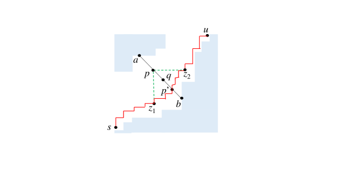
Figure 2:

Let $z_{1}$ be the first point of $\pi$ with $x-$coordinate $x_{p}$, and let $z_{2}$ be the last point of $\pi$ with $y$-coordinate $y_{p}$. How many paths $\pi^{\prime}$ through $p^{\prime}$ get mapped to the same path $\pi$ through $p$? All these paths $\pi^{\prime}$ differ only in their portion between $z_{1}$ and $z_{2}$. The number of monotone paths from $z_{1}$ to $p^{\prime}$ is at most $N\choose d$, because such a path amounts to choosing $d$ E moves out of at most $N$ steps (and some of these paths may in fact not be feasible), and similarly the number of monotone paths from $p^{\prime}$ to $z_{2}$ is at most $N\choose d$. Therefore, $n_{p^{\prime}}\leq{N\choose d}^{2}\cdot n_{p}$, for every $p^{\prime}\in qb$, and consequently $Q^{\prime}\leq{N\choose d}^{2}\cdot Q$. We have to account also for the $s-u$ paths through the query point $q$. If $|qa|>|qb|$, then we can map them to the paths through the point at distance $d$ NW of $q$, but even if $|qa|=|qb|$, note similarly that the number of paths through $q$ is at most $N^{2}$ times the number of paths through the point immediately NW of it. In any case, since $d\leq w/2$, the total number of paths before the $t$-th query is $2^{L_{t}}\leq 2{N\choose{w/2}}^{2}\cdot Q<N^{w}\cdot Q=N^{w}\cdot 2^{L_{t+1}}$. The lemma follows. ∎

The rest of the lower bound argument proceeds as follows: We shall show that there are at least $\Theta(\log N)$ decisive queries such that we can “charge” to each of them $\Theta(\log N)$ other queries — naturally, a query should be charged to only one decisive query, or at most a constant number of them. The theorem then follows immediately. The first part, the existence of $\Theta(\log N)$ decisive queries, is already obvious; the $\Theta(\log N)$ queries that can be charged to each (without much overcharging) will take a little more care to establish. We show first that there is a set of $\Omega(\log N)$ decisive queries that are $w$ far from each other in both coordinates.

Lemma 4.9.

If the total number of queries is no more than $log^{2}N$, then there is a set $S$ of $K=\Omega(\log N)$ decisive queries $\{q_{1}=(x_{1},y_{1}),\ldots,q_{K}=(x_{K},y_{K})\}$ such that, for any $1\leq i\neq j\leq K$ we have that $|x_{i}-x_{j}|,|y_{i}-y_{j}|>w$.

Proof.

Any decisive query $q_{t}=(x,y)$ takes place within a domain $D_{t}$ with a SW-most point $(\underline{x},\underline{y})$ and a NE-most point $(\bar{x},\bar{y})$. We claim that, if $x$ is within $w$ of $\underline{x},\bar{x}$, or if $y$ is within $w$ of $\underline{y},\bar{y}$, then this query decreases $L_{t}$ by at most $w\log N$. In proof, if $x$ is within $w$ of $\bar{x}$ the number of paths between $(x,y)$ and $(\bar{x},\bar{y})$ is at most ${N\choose w}\leq N^{w}$, and a similar argument holds for the other directions. Let us call such decisive queries ineffective, and otherwise they are called effective.

In summary, we have a potential function that starts at the value $N$, and then is decreased in at most $\log^{2}N$ steps either (1) by a factor of no more than two, minus additive 1 (decisive queries that are effective), or (2) by an additive term of at most $N^{\alpha}\log N$ (non-decisive, or ineffective decisive queries). It follows from arithmetic that there must be at least $\log\left({N^{1-\alpha}\over{\log^{3}N}}\right)$ queries of type (1).

Hence there is a set $S$ of $K=\Omega(\log N)$ decisive queries that are effective. At the time each of these queries was issued, it was farther than $w$ from the SW and NE corners of its domain, in both the $x$ and the $y$ direction, and thus also farther than $w$ from any other previous queries — and this includes the previous decisive queries in $S$. Hence these queries are all farther than $w$ away from each other, as claimed in the lemma. ∎

We show now how to assign $\Omega(\log n)$ non-decisive queries to each ‘effective’ query $q$ in the set $S$ of the previous lemma. These are essentially the trace of the binary search that helped the algorithm corner the adversary into $q$. We will refer in the following to the two boundary half-lines of the forbidden block generated by a non-decisive query as its walls. Consider a decisive effective query $q=(x,y)$ at time $t$.

Lemma 4.10.

For every decisive effective query point $q$ there are $\Omega(\log N)$ walls, generated by non-decisive queries, that intersect the NW-SE line through $q$ within a distance $w/2$ from $q$.

Proof.

Since the query point $q=(x,y)$ is decisive, the points $p_{1}=(x-1,y+1)$, $p_{2}=(x+1,y-1)$ that are at distance 1 NW and SE from $q$ belong to the forbidden region, hence there exist two walls within a distance of 1 from $q$ on the NW-SE line, on either side of $q$, corresponding to two queries $q_{1}=(x_{1},y_{1})$ and $q_{2}=(x_{2},y_{2})$, at times $t_{1},t_{2}$. Since $q$ is effective, the queries $q_{1},q_{2}$ are non-decisive. We will use induction on $k=2,\ldots,\lfloor\log(w/2)\rfloor$, to show that there is a set $S_{k}$ of $k$ walls, generated by non-decisive queries, that intersect the NW-SE line through $q$ on both sides, within an interval that includes the point $q$ and has length $\delta_{k}\leq 2^{k}$ (in the $L_{\infty}$ metric). This claim for $k=\lfloor\log(w/2)\rfloor$ implies immediately the lemma. For the basis, $k=2$, we let $S_{2}$ contain the walls at $p_{1}$ and $p_{2}$.

For the induction step, consider the set $S_{k}$ of walls. Let $t_{l}$ be the earliest time that generated a wall of $S_{k}$ that intersects the NW-SE line through $q$ left of $q$ (i.e. NW of $q$), let $p_{l}$ be the intersection point and $q_{l}$ the query point that generated the wall. Similarly, let $t_{r}$ be the earliest time that generated a wall of $S_{k}$ that intersects the NW-SE line through $q$ right of $q$ (i.e. SE of $q$), let $p_{r}$ be the intersection point and $q_{r}$ the query point that generated the wall.

Suppose without loss of generality that $t_{l}>t_{r}$. Why did the adversary choose SE in response to query $q_{l}$ at time $t_{l}$? Since $t_{l}>t_{r}$, the walls of $q_{r}$ existed at time $t_{l}$. The wall through $p_{l}$ is either vertical, in which case $q_{l}$ is below $p_{l}$, or the wall is horizontal, in which case $q_{l}$ is to the right of $p_{l}$ (see Figure 3). In either case, it is easy to see that the line from $q_{l}$ in the SE direction hits a wall of the query point $q_{r}$ within distance at most the length $|p_{l}p_{r}|$ of the segment $(p_{l},p_{r})$, thus at most $2^{k}$; Fig. 3 shows the geometry when the wall at $p_{r}$ is vertical (the case of a horizontal wall at $p_{r}$ is symmetric).

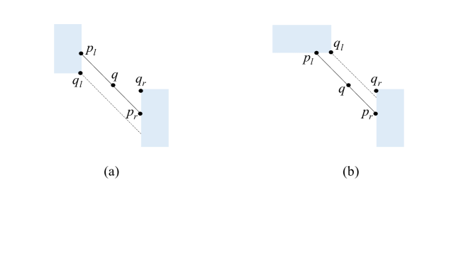
Figure 3:

Since the line from $q_{l}$ in the SE direction hits a wall within $2^{k}\leq w/2$, $q$ is a short query. Since the adversary chooses SE at $q_{l}$, the line from $q_{l}$ in the NW direction must hit also within distance at most $2^{k}$ another wall, generated by a query point $q_{k+1}$ at an earlier time $t_{k+1}<t_{l}$. Since $q_{l}$ is below or to the right of $p_{l}$, the NW-SE line through $q$ hits a wall of $q_{k+1}$ at a point $p_{k+1}$ that is at most $2^{k}$ beyond $p_{l}$. Adding this wall to $S_{k}$ yields the set $S_{k+1}$ that satisfies the induction hypothesis. ∎

We can now complete the proof of Theorem 4.7. By Lemma 4.10, to every effective decisive query $q$ we can assign $\Omega(\log N)$ non-decisive queries that generate walls within $w/2$ of $q$, hence their $x-$ or $y-$coordinate is within $w/2$ of that of $q$. Since the $\Omega(\log N)$ effective queries of the set $S$ of Lemma 4.9 are more than $w$ far from each other in both coordinates, a non-decisive query can be close to at most one query of $S$ in $x$-coordinate and at most one in $y$-coordinate. Therefore, there are $\Omega(\log^{2}N)$ distinct non-decisive queries. ∎

5 Supermodular Games

5.1 A brief intro to supermodular games

A supermodular game is a game in which the set $S_{i}$ of strategies of each player $i$ is a complete lattice, and the utility (payoff) functions $u_{i}$ satisfy certain conditions. Let $k$ be the number of players and let $S=\Pi_{i=1}^{k}S_{i}$ be the set of strategy profiles. As usual, we use $s_{i}$ to denote a strategy for player $i$ and $s_{-i}$ to denote a tuple of strategies for the other players. The conditions on the utility functions $u_{i}$ are the following:
C1. $u_{i}(s_{i},s_{-i})$ is upper semicontinuous in $s_{i}$ for fixed $s_{-i}$, and it is continuous in $s_{-i}$ for each fixed $s_{i}$, and has a finite upper bound.
C2. $u_{i}(s_{i},s_{-i})$ is supermodular in $s_{i}$ for fixed $s_{-i}$.
C3. $u_{i}(s_{i},s_{-i})$ has increasing differences in $s_{i}$ and $s_{-i}$.

A function $f:L\rightarrow{\mathbb{R}}$ is supermodular if for all $x,y\in L$, it holds $f(x)+f(y)\leq f(x\land y)+f(x\lor y)$. A function $f:L_{1}\times L_{2}\rightarrow{\mathbb{R}}$, where $L_{1},L_{2}$ are lattices, has increasing differences in its two arguments, if for all $x^{\prime}\geq x$ in $L_{1}$ and all $y^{\prime}\geq y$ in $L_{2}$, it holds that $f(x^{\prime},y^{\prime})-f(x,y^{\prime})\geq f(x^{\prime},y)-f(x,y)$.

The broader class of games with strategic complementarities (GSC) relaxes somewhat the conditions C2 and C3 into C2’, C3’ which depend only on ordinal information on the utility functions, i.e. how the utilities compare to each other rather than their precise numerical values. The supermodularity requirement of C2 is relaxed to quasi-supermodularity, where a function $f:L\rightarrow{\mathbb{R}}$ is quasi-supermodular if for all $x,y\in L$, $f(x)\geq f(x\land y)$ implies $f(y)\leq f(x\lor y)$, and if the first inequality is strict, then so is the second. The increasing differences requirement of C3 is relaxed to the single-crossing condition, where a function $f:L_{1}\times L_{2}\rightarrow{\mathbb{R}}$, satisfies the single crossing condition, if for all $x^{\prime}>x$ in $L_{1}$ and all $y^{\prime}>y$ in $L_{2}$, it holds that $f(x^{\prime},y)\geq f(x,y)$ implies $f(x^{\prime},y^{\prime})\geq f(x,y^{\prime})$, and if the first inequality is strict then so is the second. All the structural and algorithmic properties below of supermodular games hold also for games with strategic complementarities.

We will consider here games where each $S_{i}$ is a discrete (or continuous) finite box in $d_{i}$ dimensions of size $N$ in each coordinate. We let $d=\sum_{i=1}^{k}d_{i}$ be the total number of coordinates. In the discrete case, condition C1 is trivial. Condition C2 is trivial if $d_{i}=1$ (all functions in one dimension are supermodular), but nontrivial for 2 or more dimensions. C3 is nontrivial.

Supermodular games (and GSC) have pure Nash equilibria. Furthermore, the pure Nash equilibria form a complete lattice [17], thus there is a highest and a lowest equilibrium. Another important property is that the best response correspondence $\beta_{i}(s_{-i})$ for each player $i$ has the property that (1) both $\sup\beta_{i}(s_{-i})$ and $\inf\beta_{i}(s_{-i})$ are in $\beta_{i}(s_{-i})$, and (2) both functions $\sup\beta_{i}(\cdot)$ and $\inf\beta_{i}(\cdot)$ are monotone functions [24]. The function $\bar{\beta}(s)=(\sup\beta_{1}(s_{-1}),\ldots,\sup\beta_{k}(s_{-k}))$ of the supremum best responses is a monotone function from $S$ to itself, and its greatest fixed point is the highest Nash equilibrium of the game. The function $\underline{\beta}(s)=(\inf\beta_{1}(s_{-1}),\ldots,\inf\beta_{k}(s_{-k}))$ of the infimum best responses is also a monotone function, and its least fixed point is the lowest Nash equilibrium of the game.

Example 5.1.

(A simplified Diamond search model [17].)  There are $k$ players (businesses). Each player $i\in[k]$ can exert some amount of “effort”, $s_{i}\in[0,m_{i}]$, where $m_{i}>0$, to find a business partner. So, the strategy space $S_{i}$ of player $i$ is the closed bounded interval $[0,m_{i}]$. Any player $i$ incurs a cost $C_{i}(s_{i})$ for exerting effort $s_{i}$, where we assume $C_{i}(\cdot)$ is some arbitrary continuous function (we do not necessarily assume that $C_{i}(s_{i})$ is increasing in $s_{i}$; this is not needed). The payoff to player $i$ depends also on how much effort others are putting into finding a business partner. Specifically, for each player $i$, we assume that for some $\alpha_{i}>0$ the utility function $u_{i}(s_{1},\ldots,s_{k})$ for player $i$ is given by:

$$u_{i}(s):=\alpha_{i}\cdot s_{i}\cdot(\sum_{j\neq i}s_{j})-C_{i}(s_{i})$$

Let us check that this is a supermodular game. Clearly the strategy space $S_{i}=[0,m_{i}]$ of each player (a closed interval) is a complete lattice.
C1. condition C1 certainly holds, since in fact $u_{i}(s_{i},s_{-i})$ is continuous in both $s_{i}$ and $s_{-i}$, and has a finite upper bound (because the strategy spaces of all players are bounded intervals).
C2. condition C2 holds vacuously, because for fixed $s^{\prime}_{-i}$, the function $f(s_{i}):=u_{i}(s_{i},s^{\prime}_{-i})$ is a function in a single real-valued parameter, $s_{i}$, and any such function is supermodular, because for all $s_{i},s^{\prime}_{i}\in S_{i}$, $f(s_{i})+f(s^{\prime}_{i})=f(\min\{s_{i},s^{\prime}_{i}\})+f(\max\{s_{i},s^{\prime}_{i}\})=f(s_{i}\land s^{\prime}_{i})+f(s_{i}\lor s^{\prime}_{i})$.
C3. To see that condition C3 holds, i.e., that the payoff functions $u_{i}(s_{i},s_{-i})$ have increasing differences in $s_{i}$ and $s_{-i}$, suppose that $s^{\prime}_{i}\geq s_{i}$ and $s^{\prime}_{-i}\geq s_{-i}$ (coordinate-wise inequality). Then note that we have:

$$u_{i}(s^{\prime}_{i},s^{\prime}_{-i})-u_{i}(s_{i},s^{\prime}_{-i}) = \alpha_{i}s^{\prime}_{i}(\sum_{j\neq i}s^{\prime}_{j})-C_{i}(s^{\prime}_{i})-(\alpha_{i}s_{i}(\sum_{j\neq i}s^{\prime}_{j})-C_{i}(s_{i}))$$

$$= \alpha_{i}(s^{\prime}_{i}-s_{i})(\sum_{j\neq i}s^{\prime}_{j})-C_{i}(s^{\prime}_{i})+C_{i}(s_{i})$$

$$\geq \alpha_{i}(s^{\prime}_{i}-s_{i})(\sum_{j\neq i}s_{j})-C_{i}(s^{\prime}_{i})+C_{i}(s_{i})$$

$$= u_{i}(s^{\prime}_{i},s_{-i})-u_{i}(s_{i},s_{-i})$$

∎

5.2 Complexity of equilibrium computation in supermodular games

Given a supermodular game, the relevant problems include: (a) find a Nash equilibrium (anyone), and (b) find the highest or the lowest equilibrium. In the case of continuous domains, we again have to relax to an approximate solution. We assume that we have access to a best response function, e.g. $\bar{\beta}(\cdot)$ and/or $\underline{\beta}(\cdot)$, as an oracle or as a polynomial-time function. The monotonicity of these functions implies then easily the following:

Proposition 5.2.

1. The problem of computing a Nash equilibrium of a $k$-player supermodular game over a discrete finite strategy space $\Pi_{i=1}^{k}[N]^{d_{i}}$ reduces to the problem of computing a fixed point of a monotone function over $[N]^{d}$ where $d=\sum_{i=1}^{k}d_{i}$. Computing the highest (or lowest) Nash equilibrium reduces to computing the greatest (or lowest) fixed point of a monotone function.

2. For games with continuous box strategy spaces, $\Pi_{i=1}^{k}[1,N]^{d}_{i}$, and Lipschitz continuous utility functions with Lipschitz constant $K$, the problem of computing an $\epsilon$-approximate Nash equilibrium reduces to exact fixed point computation point for a monotone function with a discrete finite domain $[NK/\epsilon]^{d}$.

Proof.

1. Follows from the monotonicity of $\bar{\beta}(\cdot)$ and $\underline{\beta}(\cdot)$. If $s$ is fixed point of $\bar{\beta}(\cdot)$, then $s_{i}=\sup\beta_{i}(s_{-i})$ is a best response to $s_{-i}$ for all $i$ (since $\sup\beta_{i}(s_{-i})\in\beta_{i}(s_{-i})$), therefore $s$ is a Nash equilibrium of the game. The GFP of $\bar{\beta}(\cdot)$ is the highest Nash equilibrium. Similarly, every fixed point of $\underline{\beta}(\cdot)$ is an equilibrium of the game, and the LFP of $\underline{\beta}(\cdot)$ is the lowest equilibrium.

2. Suppose that the utility functions are Lipschitz continuous with Lipschitz constant $K$. To compute an $\epsilon$-approximate Nash equilibrium of the game, it suffices to find a $\epsilon/K$-approximate fixed point of the function $\bar{\beta}(\cdot)$. For, if $s$ is such an approximate fixed point and $s^{\prime}=\bar{\beta}(s)$, then $|s^{\prime}-s|\leq\epsilon/K$ in every coordinate. Hence $|u_{i}(s_{i},s_{-i})-u_{i}(s^{\prime}_{i},s_{-i})|\leq\epsilon$, and $s^{\prime}_{i}$ is a best response to $s_{-i}$, hence $s$ is an $\epsilon$-approximate equilibrium. Computing an $\epsilon/K$-approximate fixed point of the function $\bar{\beta}(\cdot)$ on the continuous domain, reduces by Proposition 2.2 to the exact fixed point problem for the discrete domain $[NK/\epsilon]^{d}$. ∎

Not every monotone function can be the (sup or inf) best response function of a game. In particular, a best response function has the property that the output values for the components corresponding to a player depend only on the input values for the other components corresponding to the other players. Thus, for example, for two one-dimensional players, if the function $f(x,y)$ is the best response function of a game, it must satisfy $f_{1}(x,y)=f_{1}(x^{\prime},y)$ for all $x,x^{\prime},y$, and $f_{2}(x,y)=f_{2}(x,y^{\prime})$ for all $x,y,y^{\prime}$. This property helps somewhat in improving the time needed to find a fixed point, and thus an equilibrium of the game, as noted below. For example, in the case of two one-dimensional players, an equilibrium can be computed in $O(\log N)$ time, instead of the $\Omega(\log^{2}N)$ time needed to find a fixed point of a general monotone function in two dimensions.

Theorem 5.3.

Given a supermodular game with two players with discrete strategy spaces $[N]^{d_{i}}$, $i=1,2$ with access to the sup (or inf) best response function $\bar{\beta}(\cdot)$ (or $\underline{\beta}(\cdot)$), we can compute an equilibrium in time $O((\log N)^{\min(d_{1},d_{2})})$. More generally, for $k$ players with dimensions $d_{1},\ldots,d_{k}$, an equilibrium can be computed in time $O((\log N)^{d^{\prime}})$, where $d^{\prime}=\sum_{i}d_{i}-\max_{i}d_{i}$.

Proof.

Suppose that we have access to the sup best response $\bar{\beta}(\cdot)$. Assume without loss of generality that the first player has the maximum dimension, $d_{1}=\max_{i}d_{i}$. We apply the divide-and-conquer algorithm, but take advantage of the property of the monotone function $\bar{\beta}$ that the first $d_{1}$ components of $\bar{\beta}(x)$ do not depend on the first $d_{1}$ coordinates of $x$. As a consequence, for any fixed assignment to the other coordinates, i.e. choice of a strategy profile $s_{-1}$ for all the players except the first player, the induced function on the first $d_{1}$ coordinates maps every point to the best response $\bar{\beta}_{1}(s_{-1})$ of player 1. Thus the fixed point of the induced function is simply $\bar{\beta}_{1}(s_{-1})$, it can be computed with one call to $\bar{\beta}$, and there is no need to recurse on the first $d_{1}$ coordinates. It follows that the algorithm takes time at most $O((\log N)^{d^{\prime}})$, where $d^{\prime}=\sum_{i}d_{i}-\max_{i}d_{i}$. ∎

Conversely, we can reduce the fixed point computation problem for an arbitrary monotone function to the equilibrium computation problem for a supermodular game with two players.

Theorem 5.4.

1. Given a monotone function $f$ on $[N]^{d}$ (resp. $[1,N]^{d}$) we can construct a supermodular game $G$ with two players, each with strategy space $[N]^{d}$ (resp. $[1,N]^{d}$), so that the equilibria of $G$ correspond to the fixed points of $f$.

2. More generally, the fixed point problem for a monotone function $f$ in $d$ dimensions can be reduced to the equilibrium problem for a supermodular game with any number $k\geq 2$ of players with any dimensions $d_{1},\ldots,d_{k}$, provided that $\sum_{i}d_{i}\geq 2d$ and $\sum_{i}d_{i}-\max_{i}d_{i}\geq d$.

Proof.

1. We will define the utility functions $u_{i}$ so that the best responses $\beta_{i}$ of both players are functions (i.e. are unique). For player 1, the best response will be $\beta_{1}(y)=y$, for all $y\in[N]^{d}$, and for player 2, the best response will be $\beta_{2}(x)=f(x)$, for all $x\in[N]^{d}$. If $x$ is a fixed point of $f$, then $(x,x)$ is an equilibrium of the game, since $\beta(x,x)=(x,f(x))=(x,x)$. Conversely, if $(x,y)$ is an equilibrium of the game, then $\beta(x,y)=(x,y)$, therefore $x=y$ and $y=f(x)$, hence $x=f(x)$. Thus, the set of equilibria of $G$ is $\{(x,x)|x\in Fix(f)\}$.

The utility function for player 1 is set to $u_{1}(x,y)=-(x-y)^{2}=-\sum_{j=1}^{d}(x_{j}-y_{j})^{2}$. The utility function for player 2 is $u_{2}(x,y)=-(f(x)-y)^{2}=-\sum_{j=1}^{d}(f_{j}(x)-y_{j})^{2}$. Obviously, the best response functions are as stated above, $\beta_{1}(y)=y$ and $\beta_{2}(x)=f(x)$.

The utility functions $u_{1},u_{2}$ satisfy condition C2 with equality. For example, to check $u_{2}$ ($u_{1}$ is similar), fix a $x$ and consider two values $y,y^{\prime}$. For every $j=1,\ldots,d$, we have $-(f_{j}(x)-y_{j})^{2}-(f_{j}(x)-y^{\prime}_{j})^{2}=-(f_{j}(x)-max(y_{j},y^{\prime}_{j}))^{2}-(f_{j}(x)-min(y_{j},y^{\prime}_{j}))^{2}$. Summing over all $j$ yields: $-(f(x)-y)^{2}-(f(x)-y^{\prime})^{2}=-(f(x)-max(y,y^{\prime}))^{2}-(f_{j}(x)-min(y,y^{\prime}))^{2}$.

To verify condition C3 for $u_{2}$, consider any $x^{\prime}\geq x$ and $y^{\prime}\geq y$. We have $u_{2}(x^{\prime},y^{\prime})-u_{2}(x,y^{\prime})-(u_{2}(x^{\prime},y)-u_{2}(x,y))$ $=-\sum_{j=1}^{d}(f_{j}(x^{\prime})-y^{\prime}_{j})^{2}+\sum_{j=1}^{d}(f_{j}(x)-y^{\prime}_{j})^{2}+\sum_{j=1}^{d}(f_{j}(x^{\prime})-y_{j})^{2}-\sum_{j=1}^{d}(f_{j}(x)-y_{j})^{2}$ $=\sum_{j=1}^{d}2(y^{\prime}_{j}-y_{j})(f_{j}(x^{\prime})-f_{j}(x))\geq 0$, where the last inequality holds because $y^{\prime}\geq y$ and $f(x^{\prime})\geq f(x)$ since $x^{\prime}\geq x$ and $f$ is monotone. Similarly, condition C3 can be verified for $u_{1}$.

2. Order the players in increasing order of their dimension, let $T$ be the ordering of all the $\sum_{i=1}^{k}d_{i}$ coordinates consisting first of the set $Co(1)$ of coordinates of player 1 (in any order), then the set $Co(2)$ of coordinates of player 2, and so forth. Number the coordinates in the order $T$ from 1 to $\sum_{i=1}^{k}d_{i}$, and label them cyclically with the labels $1,\ldots,d$.

We define the (unique) best response function $\beta$ as follows. For every coordinate $j\leq d$ (in the ordering $T$), we set $\beta_{j}(x)=f_{j}(x^{\prime})$, where $x^{\prime}$ is a subvector of $x$ with $d$ coordinates that have distinct labels $1,\ldots,d$ and which belong to different players than coordinate $j$. The subvector $x^{\prime}$ is defined as follows. Suppose that coordinate $j$ belongs to player $r$ ($j\in Co(r)$), and let $t=\sum_{i=1}^{r-1}d_{i}$. If $d_{r}\leq d$, then $x^{\prime}$ is the subvector of $x$ that consists of the first $t$ coordinates (in the order $T$) and the coordinates $t+1+d,\ldots,2d$; note that all these coordinates do not belong to player $r$. If $d_{r}>d$, then $r<k$ (since $\sum_{i}d_{i}-\max_{i}d_{i}\geq d$). In this case, let $x^{\prime}$ be the subvector of $x$ consisting of the last $d$ coordinates (in $T$); all of these belong to player $k\neq r$. For coordinates $j>d$, we set $\beta_{j}(x)=x_{j^{\prime}}$, where $j^{\prime}\in[d]$ is equal to $j\mod d$, unless $j^{\prime}$ belongs to the same player $r$ as $j$, in which case $d_{r}>d$, hence $r\neq k$; in this case we set $\beta_{j}(x)=x_{j"}$ for some (any) coordinate $j"$ of the last player $k$ that is labeled $j^{\prime}$.

We define the utility functions of the players so that they yield the above best response function $\beta$. Namely, we define the utility function of player $i$ to be $u_{i}(x)=-\sum_{j\in Co(i)}(x_{j}-\beta_{j}(x))^{2}$. It can be verified as in part 1 that the utility functions satisfy conditions C2 and C3. It can be easily seen also that at any equilibrium of the game, all coordinates with the same label must have the same value, and the corresponding $d$-vector $x$ is a fixed point of $f$. Conversely, for any fixed point $x$ of $f$, the corresponding strategy profile of the game is an equilibrium. ∎

Since the 2-dimensional monotone fixed point problem requires $\Omega(\log^{2}N)$ queries by Theorem 4.1, it follows that the equilibrium problem for two 2-dimensional players also requires $\Omega(\log^{2}N)$ queries, which is tight because it can be also solved in $O(\log^{2}N)$ time by Theorem 5.3. Similarly, for higher dimensions $d$, if the monotone fixed point problem requires $\Omega(\log^{d}N)$ queries then the equilibrium problem for two d-dimensional players is also $\Theta(\log^{d}N)$.

The same reduction from monotone functions to supermodular games of Theorem 5.4, combined with Proposition 2.1 implies the hardness of computing the highest and lowest equilibrium.

Corollary 5.5.

It is NP-hard to compute the highest and lowest equilibrium of a supermodular game with two 1-dimensional players with explicitly given polynomial-time best response (and utility) functions.

6 Condon’s and Shapley’s stochastic games reduce to $\mathtt{Tarski}$

In this section we show that computing the exact (rational) value of Condon’s simple stochastic games ([4]), as well as computing the (irrational) value of Shapley’s more general (stopping/discounted) stochastic games [21] to within a given desired error $\epsilon>0$ (given in binary), are both polynomial time reducible to $\mathtt{Tarski}{}$.

6.1 Condon’s simple stochastic games reduce to $\mathtt{Tarski}$

Recall that a simple stochastic game (SSG) is a 2-player zero-sum game, played on the vertices of an edge-labeled directed graph, specified by $G=(V,V_{0},V_{1},V_{2},\delta)$, whose vertices $V=\{v_{1},\ldots,v_{n}\}$ include two special sink vertices, a ${\mathbf{0}}$-sink, $v_{n-1}$, and a $\mathbf{1}$-sink, $v_{n}$, and where the rest of the vertices $V\setminus\{v_{n-1},v_{n}\}=\{v_{1},\ldots,v_{n-2}\}$ are partitioned into three disjoint sets $V_{0}$ (random), $V_{1}$ (max), and $V_{2}$ (min). The labeled directed edge relation is $\delta\subseteq(V\setminus\{v_{n-1},v_{n}\})\times((0,1]\cup\bot)\times V$. For each “random” node $u\in V_{0}$, every outgoing edge $(u,p_{u,v},v)\in\delta$ is labeled by a positive probability $p_{u,v}\in(0,1]$, such that these probabilities sum to $1$, i.e., $\sum_{\{v\in V\mid(u,p_{u,v},v)\in\delta\}}p_{u,v}=1$. We assume, for computational purposes, that the probabilities $p_{u,v}$ are rational numbers (given as part of the input, with numerator and denominator given in binary). The outgoing edges from “max” ($V_{1}$) and “min” ($V_{2}$) nodes have an empty label, “$\bot$”. We assume each vertex $u\in V\setminus\{v_{n-1},v_{n}\}$ has at least one outgoing edge. Thus in particular, for any node $u\in V_{1}\cup V_{2}$ there exists an outgoing edge $(u,\bot,v)\in\delta$ for some $v\in V$. Finally, there is a designated start vertex $s\in V$.

A play of the game transpires as follows: a token is initially placed on $s$, the start node. Thereafter, during each “turn”, when the token is currently on a node $u\in V$, unless $u$ is already a sink node (in which case the game halts), the token is moved across an outgoing edge of $u$ to the next node by whoever “controls” $u$. For a random node $u\in V_{0}$, which is controlled by “nature”, the outgoing edge is chosen randomly according to the probabilities $(p_{u,v})_{v\in V}$. For $u\in V_{1}$, the outgoing edge is chosen by player 1, the $\max$ player, who aims to maximize the probability that the token will eventually reach the $\mathbf{1}$-sink. For $u\in V_{2}$, the outgoing edge is chosen by player 2, the $\min$ player, who aims to minimize the probability that the token will eventually reach the $\mathbf{1}$-sink. The game halts if the token ever reaches either of the two sink nodes.

For every possible start node $s=v_{i}\in V$, this zero-sum game has a well defined value, $q^{*}_{i}\in[0,1]$. This is, by definition, a probability such that player 1, the max player (and, respectively, player 2, the min player) has a strategy to “force” reaching the $1$-sink with probability at least (respectively, at most) $q^{*}_{i}$, irrespective of what the other player’s strategy is. In other words, these games are determined. Moreover $q^{*}_{i}$ is a rational value whose encoding size, with numerator and denominator in binary, is polynomial in the bit encoding size of the SSG ([4]). Furthermore, both players have deterministic, memoryless (a.k.a., pure, positional) optimal strategies in the game (which do not depend on the specific start node $s$), in which for each vertex $u\in V_{1}$ (or $u\in V_{2}$) the max player (respectively the min player) chooses the same specific outgoing edge every time the token visits vertex $u$, regardless of the prior history of play prior to that visit to $u$.

Given an SSG, the goal is to compute the value of the game (starting at each vertex). Condon ([4]) already showed that the problem of deciding whether the value is $>1/2$ is in NP $\cap$ co-NP, and it is a long-standing open problem whether this is in P-time. Moreover, the search problem of computing the value for an SSG is known to be in both $\mathsf{PLS}{}$ and $\mathsf{PPAD}{}$ (see, e.g., [26] and [11]).

Proposition 6.1.

The following total search problem is polynomial-time reducible to $\mathtt{Tarski}{}$: Given an instance $G$ of Condon’s simple stochastic game, and given a start vertex $s=v_{i}\in V$, computing the exact (rational) value $q^{*}_{i}$ of the game.

Proof.

Let $x=(x_{1},\ldots,x_{n})$ be an $n$-vector of variables. The $n$-vector $q^{*}$ of values, $q^{*}_{i}$, of the SSG starting at each vertex $v_{i}$, is given by the least fixed point (LFP) solution of the following monotone min-max-linear system of $n$ equations in $n$ unknowns:

$$x_{i}=\left\{\begin{array}[]{ll}\sum_{\{v_{j}\in V\mid(v_{i},p_{v_{i},v_{j}},v_{j})\in\delta\}}p_{v_{i},v_{j}}x_{j}&\mbox{if $v_{i}\in V_{0}$}\\ \max\{x_{j}\mid(v_{i},\bot,v_{j})\in\delta\}&\mbox{if $v_{i}\in V_{1}$}\\ \min\{x_{j}\mid(v_{i},\bot,v_{j})\in\delta\}&\mbox{if $v_{i}\in V_{2}$}\\ 0&\mbox{if $v_{i}=v_{n-1}$ is the $\mathbf{0}$-sink}\\ 1&\mbox{if $v_{i}=v_{n}$ is the $\mathbf{1}$-sink}\end{array}\right.$$

We denote this system of equations by $x=F(x)$. Note that $F(x)$ defines a monotone map $F:[0,1]^{n}\rightarrow[0,1]^{n}$ mapping the complete lattice $[0,1]^{n}$ (under coordinate-wise order) to itself. Thus by Tarski’s theorem it has a least (as well as greatest) fixed point. It is well known that the least fixed point (LFP) is $q^{*}$.

Consider now the “$\beta$-discounted” (or “$\beta$-stopping”) version of these equations, $x=(1-\beta)F(x)$. where each equation now has the form $x_{i}=(1-\beta)F_{i}(x)$, for a given discount value $\beta\in(0,1)$. We can also view these equations as corresponding to a modified $\beta$-stopping version, $G^{\beta}$, of the original SSG, $G$, where at each vertex there is a direct probability $\beta$ of immediately transitioning to the $\mathbf{0}$-sink; and with the remaining probability, $(1-\beta)$, there remain exactly the same possibilities as before in $G$.)

Letting $F^{\beta}(x):=(1-\beta)F(x)$, note that $F^{\beta}:[0,1]^{n}\rightarrow[0,1]^{n}$ defines both a monotone map and a contraction map with respect to the $l_{\infty}$ norm. Specifically, for $x,y\in[0,1]^{n}$, $\|F^{\beta}(x)-F^{\beta}(y)\|_{\infty}\leq(1-\beta)\|x-y\|_{\infty}$. Hence, by Banach’s fixed point theorem, $x=F^{\beta}(x)$ has a unique fixed point solution, $q^{\beta}\in[0,1]^{n}$ (which is also both the least and greatest fixed point of $x=F^{\beta}(x)$ in $[0,1]^{n}$). The vector $q^{\beta}$ corresponds to the game values of the $\beta$-stopping game $G^{\beta}$, starting at each vertex.

Let $|G|$ denote the bit encoding size of the given SSG, $G$. There is a fixed polynomial, $h()$ such that for any SSG, $G$, the denominator of the rational values $q^{*}_{i}$ is at most $2^{h(|G|)}$. If we apply this to the already $\beta$-discounted SSG, $G^{\beta}$, then this says that the denominators of the values $q^{\beta}_{i}$ are at most $2^{h(|G|+\log(1/\beta))}$.

Moreover, for any SSG $G$, there is also a fixed polynomial, $r(x)$, such that given a rational vector $q^{\prime}\in[0,1]^{n}$, such that $\|q^{*}-q^{\prime}\|_{\infty}<2^{-r(|G|)}$, the closest rational number to $q^{\prime}_{i}$ with denominator at most $2^{h(|G|)}$ is $q^{*}_{i}$.

It is also known (see, e.g., Lemma 8 in [4]) that there is some fixed polynomial $t(\cdot)$, such that if $\beta=\epsilon 2^{-t(|G|)}$, for any $\epsilon\in(0,1)$, then $\|q^{*}-q^{\beta}\|_{\infty}<\epsilon/2$.

Thus if we let $\epsilon=2^{-r(|G|)}$, and $\beta=\epsilon 2^{-t(|G|)}$, then not only do we have $\|q^{*}-q^{\beta}\|_{\infty}<2^{-r(|G|)}$, but we also have that, for all $i\in[n]$, the closest rational number to $q^{\beta}_{i}$ with denominator at most $2^{h(|G|)}$ is $q^{*}_{i}$.

Next we note that for $\beta=2^{-w(|G|)}$, where $w(x):=r(x)+t(x)$ is a polynomial, the map $F^{\beta}:[0,1]^{n}\rightarrow[0,1]^{n}$ defines a polynomially contracting function, as defined in [11], because for all $x,y\in[0,1]^{n}$, $\|F^{\beta}(x)-F^{\beta}(y)\|_{\infty}<(1-\beta)\|x-y\|_{\infty}$. In other words, the Lipschitz constant for the contraction map has the form $(1-\frac{1}{2^{poly(|I|)}})$, where $|I|$ denotes the bit encoding size of the input $I$ that describes the map. Hence, it follows from Proposition 2.2, part (3.) of [11] that in order to compute some $q^{\prime}\in[0,1]^{n}$ such that $\|q^{\beta}-q^{\prime}\|_{\infty}<\epsilon/2$, for some desired $\epsilon\in(0,1)$, it suffices to compute some $q^{\prime}\in[0,1]^{n}$ such that $\|F^{\beta}(q^{\prime})-q^{\prime}\|_{\infty}<(\epsilon/2)\beta$.

Combining the above facts together it follows that, given an SSG, $G$, computing its vector of values $q^{*}$ is P-time reducible to computing a vector $q^{\prime}\in[0,1]^{n}$ such that $\|F^{\beta}(q^{\prime})-q^{\prime}|<\frac{1}{2^{z(|G|)}}$, where $\beta=2^{-w(|G|)}$, and where $z(x):=w(x)+r(x)=t(x)+2\cdot r(x)$, is a fixed polynomial.

We next show that, given $G$, the problem of computing such a vector $q^{\prime}\in[0,1]^{n}$ is reducible to $\mathtt{Tarski}$. Note, firstly, that for $\beta=2^{-w(|G|)}$, $F^{\beta}(x)$ is polynomial-time computable, given the rational vector $y\in[0,1]^{n}$, and given the underlying SSG $G$.

We now define a discrete monotone function $H:[M]^{n}\rightarrow[M]^{n}$, such that $H()$ is a discretization of the monotone contraction map $F^{\beta}()$, where $\beta=2^{-w(|G|)}$, such that any fixed point of $H$ directly yields (via rescaling) a vector $q^{\prime}\in[0,1]^{n}$ such that $\|F^{\beta}(q^{\prime})-q^{\prime}|<2^{-z(|G|)}$.

The map $H()$ is defined as follows. We let $M=2^{2\cdot z(|G|)}$. For $v\in[M]^{n}$, we let $H(v)_{i}=\lfloor M\cdot F^{\beta}(v/M)_{i}\rfloor$, for all $i\in[n]$. Clearly, $H:[M]^{n}\rightarrow[M]^{n}$ defines a monotone map which is polynomial-time computable, given the input vector $v\in[M]^{n}$ and given the SSG, $G$. Moreover, if we find some fixed point $v^{*}\in[M]^{n}$ such that $v^{*}=H(v^{*})$, then $\|F^{\beta}(v^{*}/M)-v^{*}/M\|_{\infty}<2^{-z(|G|)}$. Hence, a fixed point $v^{*}$ of $H$ immediately yields a vector $q^{\prime}\in[0,1]^{n}$ such that $\|F^{\beta}(q^{\prime})-q^{\prime}\|_{\infty}<2^{-z(|G|)}$, given which we know we can compute $q^{*}$ in P-time. We have therefore shown that the problem of computing the vector $q^{*}\in[0,1]^{n}$ of values for a given SSG, $G$, is P-time reducible to $\mathtt{Tarski}{}$. ∎

6.2 Shapley’s stochastic games reduce to $\mathtt{Tarski}$

We now consider the original stochastic games introduced by Shapley in [21], which are more general than Condon’s games, and show that approximating the value of such a game (which is in general irrational, even when the input data associated with the game consists of rational numbers), to within any given desired accuracy, $\epsilon>0$ (given in binary as part of the input), is polynomial time reducible to $\mathtt{Tarski}$.

Shapley’s games are a class of two-player zero-sum “stopping”, or equivalently “discounted”, stochastic games. An instance of Shapley’s stochastic game is given by $G=(V,A,P,s)$, where $V=\{v_{1},\ldots,v_{n}\}$ is a set of $n$ vertices (or “states”). For each vertex, $v_{i}\in V$, there is an associated $m_{i}\times n_{i}$ reward matrix, $A^{i}$, where $m_{i}$ and $n_{i}$ are positive integers denoting, respectively, the number of distinct “actions” available to player 1 (the maximizer) and player 2 (the minimizer) at vertex $v_{i}$, and where for each pair of such actions, $j\in[m_{i}]$ and $k\in[n_{i}]$, $A^{i}_{j,k}\in{\mathbb{Q}}$ is a reward for player 1 (which we assume, for computational purposes, is a rational number given as input by giving its numerator and denominator in binary). Furthermore, for each vertex $v_{i}\in V$, and each pair of actions $j\in[m_{i}]$ and $k\in[n_{i}]$, $P^{i}_{j,k}\in[0,1]^{n}$ is a vector of probabilities on the vertices $V$, such that $0\leq P^{i}_{j,k}(r)$, and $\sum_{r=1}^{n}P^{i}_{j,k}(r)<1$, i.e., the probabilities sum to strictly less than $1$. Again, we assume each such probability $P^{i}_{j,k}(r)\in{\mathbb{Q}}$ is a rational number given as input in binary. Finally, the game specifies a designated start vertex $s\in V$.

A play of Shapley’s game transpires as follows: a token is initially placed on $s$, the start node. Thereafter, during each “round” of play, if the token is currently on some node $v_{i}\in V$, both players simultaneously and independently choose respective actions $j\in[m_{i}]$ and $k\in[n_{i}]$, and player 1 then receives the corresponding reward $A^{i}_{j,k}$ from player 2; thereafter, for each $r\in[n]$ with probability $P^{i}_{j,k}(r)$ the token is moved from node $v_{i}$ to node $v_{r}$, and with the remaining positive probability $q^{i}_{j,k}=1-\sum_{r=1}^{n}P^{i}_{j,k}(r)>0$, the game “halts”. Let $q=\min\{q^{i}_{j,k}\mid i,j,k\}>0$ be the minimum such halting probability at any state, and under any pair of actions. Since $q$ is positive, i.e., since there is positive probability $\geq q>0$ of halting after each round, a play of the game eventually halts with probability 1. The goal of player 1 (player 2) is to maximize (minimize, respectively) the expected total reward that player 1 receives from player 2 during the entire play. A strategy for each player specifies, based in principle on the entire history of play thusfar, a probability distribution on the actions available at the current token location. Given strategies $\sigma_{1}$ and $\sigma_{2}$ for player 1 and 2, respectively, let $r_{i}(\sigma_{1},\sigma_{2})$ denote the expected total payoff to player 1, starting at node $s=v_{i}\in V$. Shapley [21] showed that these games have a value, meaning that $\sup_{\sigma_{1}}\inf_{\sigma_{2}}r_{i}(\sigma_{1},\sigma_{2})=\inf_{\sigma_{2}}\sup_{\sigma_{1}}r_{i}(\sigma_{1},\sigma_{2})$. In fact, Shapley showed that both players have optimal stationary (but randomized) strategies in such games, i.e., optimal strategies that only depend on the current node where the token is located, not the prior history of play, but where players can randomize on their choice of actions at each node.

Let $r^{*}_{i}=\sup_{\sigma_{1}}\inf_{\sigma_{2}}r_{i}(\sigma_{1},\sigma_{2})$ denote the game value starting at vertex $s=v_{i}\in V$.

Proposition 6.2.

The following total search problem is polynomial-time reducible to $\mathtt{Tarski}$: Given an instance $G$ of Shapley’s stochastic game, and given $\epsilon>0$ (in binary), compute a vector $r^{\prime}\in{\mathbb{Q}}^{n}$ such that $\|r^{*}-r^{\prime}\|_{\infty}<\epsilon$.

Proof.

For a matrix $B\in{\mathbb{R}}^{m_{i}\times n_{i}}$, let $\mathsf{Val}(B)$ denote the von Neumann minimax value of the corresponding 2-player zero-sum (one-shot) matrix game defined by $B$. Shapley showed that for an instance $G$ of his stochastic game, the $n$-vector $r^{*}\in{\mathbb{R}}^{n}$ of values starting at each vertex is the unique solution to the following system of $n$ equations in $n$ unknowns $x=(x_{1},\ldots,x_{n})$. For each vertex $v_{i}\in V$, define the $m_{i}\times n_{i}$ matrix $B^{i}(x)$ whose $(j,k)$-entry is $B^{i}(x)_{j,k}=A^{i}_{j,k}+\sum_{r=1}^{n}P^{i}_{j,k}(r)x_{r}$. The equations are given by:

$$x_{i}=\mathsf{Val}(B^{i}(x))\quad\mbox{for all $i\in[n]$}$$

Denote this system of equations by $x=F(x)$. If we let $M=max_{i,j,k}|A^{i}_{j,k}|$ denote the maximum absolute value reward, then it is easy to observe that $F(x)$ defines a map

$$F:\left[\frac{-M}{q},\frac{M}{q}\right]^{n}\rightarrow\left[\frac{-M}{q},\frac{M}{q}\right]^{n}$$

from $\left[\frac{-M}{q},\frac{M}{q}\right]^{n}$ to itself, and moreover, as Shapley observed, $F(x)$ is a contraction map with respect to the $l_{\infty}$ norm. Specifically, for any $x,y\in\left[\frac{-M}{q},\frac{M}{q}\right]^{n}$, $\|F(x)-F(y)\|_{\infty}\leq(1-q)\|x-y\|_{\infty}$. In other words, the Lipschitz constant of the contraction map is $(1-q)$. (Hence, $F(x)$ is a polynomially contracting function, as defined in [11].)

Hence, by Banach’s fixed point theorem, $F(x)$ has a unique fixed point in $\left[\frac{-M}{q},\frac{M}{q}\right]^{n}$. Shapley showed that the unique fixed point is indeed the vector of game values $r^{*}$, i.e., that $r^{*}=F(r^{*})$ and $r^{*}\in\left[\frac{-M}{q},\frac{M}{q}\right]^{n}$. Furthermore, $F(x)$ is also clearly a monotone function, even when the rewards $A^{i}_{j,k}$ can take on negative values. This is because the rewards only play an additive role in the entries $B^{i}(x)_{j,k}=A^{i}_{j,k}+\sum_{r=1}^{n}P^{i}_{j,k}(r)x_{r}$ of the matrices $B^{i}(x)$, and the coefficient $P^{i}_{i,k}(r)$ of each variable $x_{r}$ is non-negative (it is a probability), and because the minimax value operator $\mathsf{Val}(\cdot)$ is a monotone operator. In other words, for any two matrices $B,B^{\prime}\in{\mathbb{R}}^{m_{i}\times n_{i}}$, if $B\leq B^{\prime}$ (entry-wise inequality), then clearly $\mathsf{Val}(B)\leq\mathsf{Val}(B^{\prime})$.

Thus $r^{*}$ is both the unique fixed point solutions of the polynomially contracting map $F(x)$, as well as the (least and greatest) fixed point solution of the monotone (Tarski) map $F(x)$. Furthermore, $F(x)$ is a polynomial-time computable map: given the input game $G$, and given a rational vector $b\in{\mathbb{Q}}^{n}$ (with entries encoded in binary), we can compute $F(b)$ in time polynomial in the total bit encoding size of $G$ and $b$.

Thus, just as in the case of the functions $F^{\beta}(x)$ that arose for showing that computing the value of Condon’s stochastic games reduces to Tarski, it follows from the from [11] (Proposition 2.2, part (3.)), that in order to compute a vector $r^{\prime}\in\left[\frac{-M}{q},\frac{M}{q}\right]^{n}$, such that $\|r^{*}-r^{\prime}\|_{\infty}<\epsilon$, it suffices to compute $r^{\prime}$ such that $\|F(r^{\prime})-r^{\prime}\|_{\infty}<\epsilon\cdot q$.

Hence, again as in the proof for Condon’s game, this allows us to “discretize” the monotone function $F()$, to turn the problem of computing such a vector $r^{\prime}$ into an instance of $\mathtt{Tarski}{}$. Specifically, for a positive integer $K$, let $\langle K\rangle=\{-K,-K+1,\ldots,1,0,1,\ldots,K-1,K\}$. We construct a discrete monotone map, $H^{\prime}:\langle M^{\prime}\rangle^{n}\rightarrow\langle M^{\prime}\rangle^{n}$, where $M^{\prime}=4M/(\epsilon\cdot q)$. For $v\in\langle M^{\prime}\rangle^{n}$, we let $H^{\prime}(v)_{i}=\lfloor M^{\prime}\cdot F(v/M^{\prime})_{i}\rfloor$, for all $i\in[n]$. $H^{\prime}$ defines a monotone map which is polynomial-time computable, given the input vector $v\in\langle M^{\prime}\rangle^{n}$, given the instance $G$ of Shapley’s stochastic game, and given the desired error $\epsilon>0$ (in binary). Moreover (again, as in the case for Condon’s game), if we find a fixed point $v^{*}\in\langle M^{\prime}\rangle^{n}$ such that $v^{*}=H^{\prime}(v^{*})$, then $\|F(v^{*}/M^{\prime})-v^{*}/M^{\prime}\|_{\infty}\leq\epsilon\cdot q$, and hence $\|r^{*}-v^{*}/M^{\prime}\|_{\infty}<\epsilon$.

Hence we have shown that approximating the value vector $r^{*}$, for a given instance $G$ of Shapley’s stochastic game, within a given desired additive error $\epsilon>0$ (given in binary), is polynomial-time reducible to $\mathtt{Tarski}$. ∎

7 Conclusions

We have studied the complexity of computing a Tarski fixed point for a monotone function over a finite discrete Euclidean grid, and we have shown that this problem essentially captures the complexity of computing a ($\epsilon$-approximate) pure Nash equilibrium of a supermodular game. We have also shown that computing the value of Condon’s and Shapley’s stochastic games reduces to this $\mathtt{Tarski}$ fixed point problem, where the monotone function is given succinctly (by a boolean circuit).

We have provided several upper bounds for the $\mathtt{Tarski}$ problem, showing that it is contained in both $\mathsf{PLS}{}$ and $\mathsf{PPAD}$. On the other hand, in the oracle model, for 2-dimensional monotone functions $f:[N]^{2}\rightarrow[N]^{2}$, we have shown a $\Omega(\log^{2}N)$ lower bound for the (expected) number of (randomized) queries required to find a Tarski fixed point, which matches the $O(\log^{d}N)$ upper bound for $d=2$.

A key question left open by our work is to improve the lower bounds in the oracle model to higher dimensions. It is tempting to conjecture that for any dimension $d<\log N$, a lower bound close to $\Omega(\log^{d}N)$ holds. On the other hand, we know that this cannot hold for arbitrary $d$ and $N$, because we also have the $dN$ upper bound (which is better than $\log^{d}N$ when $d=\omega(\log N)$).

Another interesting open question is the relationship between the $\mathtt{Tarski}$ problem and the total search complexity class $\mathsf{CLS}{}$ [9], as well as the closely related recently defined class $\mathsf{EOPL}$ (which stands for “End of Potential Line” [13, 14]). $\mathsf{EOPL}{}$ is contained in $\mathsf{CLS}{}$, which is contained in both $\mathsf{PLS}$ and $\mathsf{PPAD}$. Is $\mathtt{Tarski}$ in $\mathsf{CLS}$ (or in $\mathsf{EOPL}{}$)? That would be remarkable, as the proof that it is in $\mathsf{PPAD}$ is currently quite indirect. Conversely, can $\mathtt{Tarski}$ be proved to be $\mathsf{CLS}{}$-hard ($\mathsf{EOPL}{}$-hard)? (Recall from the previous section that some key problems in $\mathsf{CLS}{}$ related to stochastic games do reduce to $\mathtt{Tarski}$.)

Another question worth considering is the complexity of the $\mathtt{unique}{}$-$\mathtt{Tarski}{}$ problem, where the monotone function is further assumed (promised) to have a unique fixed point. Is $\mathtt{unique}$-$\mathtt{Tarski}{}$ easier than $\mathtt{Tarski}{}$? Note that our $\Omega(\log^{2}N)$ lower bound in the oracle model, in dimension $d=2$, applies on the family of “herringbone” functions which do have a unique fixed point.

Acknowledgements

Thanks to Alexandros Hollender for pointing us to [2].

References

- [1] K. J. Arrow and G. Debreu. Existence of an equilibrium for a competitive economy. Econometrica, pages 265–290, 1954.
- [2] S. R. Buss and A. S. Johnson. Propositional proofs and reductions between NP search problems. Annals of Pure and Applied Logic, volume 163, pp. 1163–1182, 2012.
- [3] C.-L. Chang, Y.-D. Lyuu, and Y.-W. Ti. The complexity of Tarski’s fixed point theorem. Theoretical Computer Science, volume 401, pp. 228-235, 2008.
- [4] A. Condon. The complexity of stochastic games. Information and Computation, volume 96, pp. 203–224, 1992.
- [5] C. Dang, Q. Qi, and Y. Ye. Computational models and complexities of Tarski’s fixed points. Technical Report, Stanford University, 2012.
- [6] C. Dang and Y. Ye. On the complexity of an expanded Tarski’s fixed point problem under the componentwise ordering. Theoretical Computer Science, volume 732, pp. 26–45, 2018.
- [7] C. Dang and Y. Ye. On the complexity of a class of Discrete Fixed Point Problems under the Lexicographic Ordering. Technical Report, City University of Hong Kong, CY2018-3, 17 pages, 2018.
- [8] C. Dang and Y. Ye. Personal commuication with the authors. March, 2019.
- [9] C. Daskalakis and C. H. Papadimitriou. Continuous Local Search. In Proceedings of 22nd ACM-SIAM Symp. on Discrete Algorithms (SODA), pages 790–804, 2011.
- [10] F. Echenique. Finding all equilibria in games with strategic complements. Journal of Economic Theory, 135(1):514-532, 2007.
- [11] K. Etessami and M. Yannakakis. On the complexity of Nash equilibria and other fixed points. Siam Journal on Computing, 39(6):2531-2597, 2010.
- [12] K. Etessami and M. Yannakakis. Recursive Markov decision processes and recursive stochastic games. Journal of the ACM, 62(2), 69 pages, 2015.
- [13] J. Fearnley, S. Gordon, R. Mehta, and R. Savani. End of Potential Line. arXiv preprint 1804.03450, 54 pages, 2018.
- [14] J. Fearnley, S. Gordon, R. Mehta, and R. Savani. Unique End of Potential Line. In Proc. of 46th Int. Coll. on Automata, Languages, and Programming (ICALP’19), 15 pages, 2019. (Full preprint: arXiv:1811.03841, 90 pages, 2018.)
- [15] H. Freudenthal. Simplizialzerlegungen von beschrankter flachheit. Annals of Mathematics, vol. 43, pp. 580-582, 1942.
- [16] D. S. Johnson, C. H. Papadimitriou, M. Yannakakis. How easy is local search? Journal of Computer and System Sciences, vol. 37, pages 79-100, 1988.
- [17] P. Milgrom and J. Roberts. Rationalizability, learning, and equilibrium in games with strategic complementarities. Econometrica, pages 1255-1277, 1990.
- [18] J. Nash. Non-cooperative Games. Annals of Mathematics, pages 286–295, 1951.
- [19] N. Nisan, T. Roughgarden, E. Tardos, and V. V. Vazirani (editors). Algorithmic Game Theory. Cambridge University Press, 2007.
- [20] C. H. Papadimitriou. On the Complexity of the Parity Argument and Other Inefficient Proofs of Existence. Journal of Computer and System Sciences, 48(3):498-532, 1994.
- [21] L. S. Shapley. Stochastic Games. Proceeding of the National Academy of Sciences, volume 39(10), pages 1095–1100, 1953.
- [22] A. Tarski. A lattice-theoretical fixpoint theorem and its applications. Pacific Journal of Mathematics, volume 5(2), pages 285–309, 1955.
- [23] D. M. Topkis. Equilibrium Points in Nonzero-Sum n-Person Submodular Games. SIAM Journal on control and optimization, volume 17(6), pages 773–787, 1979.
- [24] D. M. Topkis. Supermodularity and Complementarity. Princeton University Press, 2011.
- [25] M. Yannakakis. Computational complexity (Chapter 2). Local Search in Combinatorial Optimization. (Edited by E. Aarts and J. K. Lenstra.), John Wiley & Sons, 1997.
- [26] M. Yannakakis. The analysis of local search problems and their heuristics. In Proc. of Symp. on Theoretical Aspects of Computer Science (STACS), LNCS 415, Springer, pp. 298–311, 1990.