A study of Kepler supernova remnant: angular power spectrum estimation from radio frequency data

Abstract

Supernova remnants (SNRs) have a variety of overall morphology as well as rich structures over a wide range of scales. Quantitative study of these structures can potentially reveal fluctuations of density and magnetic field originating from the interaction with ambient medium and turbulence in the expanding ejecta. We have used $1.5$GHz (L band) and $5$GHz (C band) VLA data to estimate the angular power spectrum $C_{\ell}$ of the synchrotron emission fluctuations of the Kepler SNR. This is done using the novel, visibility based, Tapered Gridded Estimator of $C_{\ell}$. We have found that, for $\ell=(1.9-6.9)\times 10^{4}$, the power spectrum is a broken power law with a break at $\ell=3.3\times 10^{4}$, and power law index of $-2.84\pm 0.07$ and $-4.39\pm 0.04$ before and after the break respectively. The slope $-2.84$ is consistent with 2D Kolmogorov turbulence and earlier measurements for the Tycho SNR. We interpret the break to be related to the shell thickness of the SNR ($0.35$ pc) which approximately matches $\ell=3.3\times 10^{4}$ (i.e., $0.48$ pc). However, for $\ell>6.9\times 10^{4}$, the estimated $C_{\ell}$ of L band is likely to have dominant contribution from the foregrounds while for C band the power law slope $-3.07\pm 0.02$ is roughly consistent with $3$D Kolmogorov turbulence like that observed at large $\ell$ for Cas A and Crab SNRs.

1 Introduction

A supernova explosion marks the end stage of the life cycle of a massive star. The huge amount of kinetic energy released during the explosion, moves through the surrounding interstellar medium (ISM) in the form of a shock wave. As the shock travels ahead of the ejected stellar material, it collects materials from the ISM through heating and compression. When the mass swept up by the shock becomes almost comparable to that of the ejecta, the remnant enters into its adiabatic phase. This is generally characterized by a spherically symmetric model which assumes an isotropic explosion in a homogeneous ambient medium. This simplistic assumption leads to a self-similar solution which was given independently by Sedov (1946) and Taylor (1950), for any strong point-like explosion. However, the one-dimensional self-similarity does not remain valid for other phases of evolution due to the interaction of the ejecta with the inhomogeneities in the ISM (Chevalier, 1977).

Besides the temporal evolution, at any epoch a supernova remnant (SNR) exhibits a variety of rich and complex structure across a wide range of length scale and frequency of observation. At radio wavelengths, the dominant contribution to the SNR emission comes from the non-thermal synchrotron radiation, emitted by relativistic electrons spiralling in the magnetic field. A plausible hypothesis (Gull, 1973) is that the interaction between the ISM and the ejecta amounts to a convective instability, which makes sufficient turbulent energy available to account for the observed synchrotron radio emission. It is difficult to identify each underlying source of turbulence and precisely quantify its nature. However, the statistical quantification of the observed intensity fluctuations in the synchrotron radiation is expected to reveal interesting information about the fine spatial structures in the remnant.

Roy et al. (2009) have carried out a power spectrum analysis of the intensity fluctuations for two supernova remnants, Cas A and Crab. The power spectrum was estimated directly from the visibilities measured in the radio interferometric observations from Very Large Array (VLA) at frequencies $~{}1.5$ GHz (L band) and $~{}5$ GHz (C band). The estimator correlated pairs of visibilities (see Bare Estimator of Choudhuri et al. (2014)) and the resultant power spectrums of the SNRs were found to follow approximately a power law of index $-3.24\pm 0.03$. A break in power law from $-3.2$ to $-2.2$ was noted for Cas A owing to the shell-type structure of the remnant. Moreover, no such change in the power law of the power spectrum was observed for filled-type geometry of Crab. These power law power spectrums were shown to be roughly consistent with MHD turbulence in the synchrotron emitting plasma. For Tycho SNR, a Kolmogorov-like magnetic energy spectrum has been reported by analysing the spatial two-point correlation function of synchrotron intensities (Shimoda et al., 2018).

In this paper, we estimate the angular power spectrum of the Kepler SNR using two different VLA archival visibility data observed in the L and C bands respectively. We use an improved estimator Tapered Gridded Estimator (TGE) (Choudhuri et al., 2016b) which helps in computing the angular power spectrum directly from the visibilities by efficiently gridding the data, thereby reducing the computational time. This gridding property is not particularly important here since we handle a small amount of data. The estimator gives an added advantage of suppressing the residual point source contamination to a large extent by tapering the primary beam response through an appropriate convolution in the visibility domain. We also present the angular power spectrum estimates of Cas A and Crab as consistency checks for the estimator and to verify the results reported in Roy et al. (2009).

Kepler’s supernova (SN1604) was first recorded by Johannes Kepler. $5$GHz results at Cambridge and at Owens valley, revealed that Kepler SNR has a shell structure of $170\arcsec$ diameter, almost circular, but with irregular brightness distribution i.e brightest in the North, with a gap in the South and a peculiar dent in the East and the remnant is quite similar to Tycho’s SNR in term of its age, size, flux density and radio structure (Gull, 1975). Kepler SNR is estimated to be located at a distance of $(4.8-6.4)$ kpc (Reynoso & Goss, 1999) using VLA H i observations of the remnant. The remnant is believed to be a result of type Ia explosion. From deep Chandra observations, Reynolds et al. (2007) confirmed the high Fe/O ratio and found no evidence for a neutron star, further supporting the Type Ia origin. Patnaude et al. (2012) claimed that Kepler SNR was likely to be a $91$T-like event that produced nearly $1M_{\sun}$ ⁵⁶Ni, by comparing the observed X-ray spectrum with simulated spectra based on their hydrodynamic modeling. By simply comparing the X-ray spectra, Katsuda et al. (2015) found that line intensity ratios of iron-group elements (IGE) to intermediate-mass elements (IME) for Kepler SNR and SNR $0509-67.5$ are much higher than those for Tycho SNR and therefore argued that Kepler SNR is the product of an overlumious Type Ia SNe.

We present the estimates of the angular power spectrum of the observed intensity fluctuations from the VLA archival data of the Kepler SNR using TGE. The details of the archival data used here and its analysis technique are briefly outlined in Section 2. The methodology of the power spectrum estimation and its error are described in Section 3. We discuss the results of Cas A, Crab SNR in Section 4. We present the results of Kepler SNR in Section 5, followed by its discussion and conclusion in Section 6.

2 Data

We use multi-configuration archival data (details given in Table 1) of VLA observations of Kepler SNR in the L and C frequency bands. Here we reduce the single frequency and line-free channel data of Kepler SNR in each configuration using the standard tasks (Wilson et al. (2013), Thompson et al. (2017)) in classic AIPS. The bad visibility points are flagged following which the flux density scale and instrumental phase are calibrated. The calibrated visibility data of the target source is subsequently separated from the multi-source uv data of a given configuration using the task SPLIT. We convert the calibrated visibilities of the SNR into a CLEANed radio image (shown in Figure 1) to verify the flagging and calibration. The angular diameter of the remnant is inferred from the image along the north-south and east-west directions by identifying the boundary of the remnant. The approximate mean diameter evaluated for Kepler SNR are $3.70\arcmin$ and $3.30\arcmin$ in L and C bands respectively.

Band	Array	Observation date	Bandwidth (MHz)	ToS (mins)	Central frequency (GHz)
C	A	2004 December 17	25	318	IF1 : 4.7149, IF2: 4.9851
C	B	2005 March 8	50	245	IF1 : 4.7149, IF2: 4.9851
C	C	2004 May 6	50	165	IF1 : 4.7149, IF2: 4.9851
L	A	2004 December 19	25	319	IF1 : 1.4649, IF2: 1.3649
L	B	2005 April 27	50	216	IF1 : 1.4649, IF2: 1.3649
L	C	2004 May 6	50	165	IF1 : 1.2851, IF2: 1.4649

Table 1: Specifications of the VLA archival data for Kepler SNR bearing project code AD$498$. The fifth column ToS stands for the total on-source time.

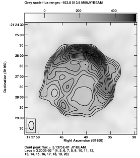
Figure 1: Total intensity contour plots of the Kepler SNR obtained using AIPS from the calibrated visibility data set of C (left) and L (right) bands respectively. Only the VLA C configuration data were used for both the plots.

3 Methodology

3.1 Power spectrum estimation using TGE

We apply the visibility based TGE (details in Choudhuri et al. (2014, 2016b)) to the calibrated visibility data of the SNR to estimate the angular power spectrum $C_{\ell}$ of the measured brightness temperature fluctuations. Each measured visibility $\mathcal{V}_{i}$ is assumed to be the sum of two contributions namely the sky signal $\mathcal{S}(\textbf{{U}}_{\rm i})$ and a system noise contribution $\mathcal{N}_{i}$

$$\mathcal{V}_{i}=\mathcal{S}(\textbf{{U}}_{\rm i})+\mathcal{N}_{i}\,.$$ (1)

The signal component $\mathcal{S}(\textbf{{U}}_{\rm i})$ is the Fourier transform of the product of the telescope’s primary beam pattern $\textit{A}(\bm{\theta})$ and the brightness temperature fluctuations $\delta\textit{T}(\bm{\theta})$ on the sky (eg. eq. ($10.2.10$) of Chengalur et al. 2003)

$$\mathcal{S}(\textbf{{U}}_{\rm i})=Q_{\nu}\int d^{2}\bm{\theta}\,e^{2\pi i\textbf{{U}}_{\rm i}\cdot\bm{\theta}}\,\textit{A}(\bm{\theta})\,\delta\textit{T}(\bm{\theta})$$ (2)

where $\bm{\theta}$ is a 2D vector in the plane of the sky with $\theta=\mid\bm{\theta}\mid$. Here $Q_{\nu}=2k_{B}/\lambda^{2}$ is the conversion factor from brightness temperature to specific intensity in the Rayleigh Jeans limit and $k_{B}$ is the Boltzmann constant. Eq. (2) can also be written in terms of a convolution as

$$\mathcal{S}(\textbf{{U}}_{\rm i})=Q_{\nu}\int d^{2}{\textbf{{U}}}\,\tilde{a}(\textbf{{U}}_{\rm i}-\textbf{{U}})\,\Delta\tilde{T}(\textbf{{U}})$$ (3)

where $\tilde{a}(\textbf{{U}})$ and $\Delta\tilde{T}(\textbf{{U}})$ are the Fourier transforms of $\textit{A}(\bm{\theta})$ and $\delta\textit{T}(\bm{\theta})$ respectively. Here we assume that the observed sky signal $\delta\textit{T}(\bm{\theta})$ is a particular realization of a statistically homogeneous and isotropic Gaussian random field whose statistical properties are completely quantified by the angular power spectrum $C_{\ell}$ defined using

$$\langle\Delta\tilde{T}(\textbf{{U}})\,\Delta\tilde{T}^{*}(\textbf{{U}}^{{}^{\prime}})\rangle=\delta^{2}_{D}(\textbf{{U}}-\textbf{{U}}^{{}^{\prime}})\,C_{2\pi U}$$ (4)

where the angular brackets denotes an ensemble average over different realizations of the random field $\delta\textit{T}(\bm{\theta})$. The estimator here aims to determine $C_{\ell}$ from $\mathcal{V}_{i}$ the measured visibilities.

The primary beam pattern $\textit{A}(\bm{\theta})$ quantifies how the individual antenna responds to signals from different directions $\bm{\theta}$ in the sky. The primary beam pattern $\textit{A}(\bm{\theta})$ typically has a full width at half maxima $(\theta_{FWHM})$ of $\sim\lambda/D$ where $D$ is the antenna diameter, and for example $\theta_{FWHM}\sim 30^{\arcmin}$ for VLA in the L band. The target source one wishes to observe is usually smaller than the angular extent of $\textit{A}(\bm{\theta})$, and for example it is $\sim 3^{\arcmin}$ for the Kepler SNR. In addition to the sky signal from the target source, the measured visibilities $\mathcal{V}_{i}$ may have significant contributions from other sources which lie within the angular extent of $\textit{A}(\bm{\theta})$. It is therefore desirable to restrict the sky response to a small region around the target source and thereby avoid contributions from extraneous sources. The TGE achieves this by tapering the sky response with a suitably chosen window function $\textit{W}(\bm{\theta})$. Here we have used $\textit{W}(\bm{\theta})=e^{-\theta^{2}/\theta_{w}^{2}}$ with $\theta_{w}=0.6\,f\,\theta_{FWHM}$ where the parameter $0<f\leq 1$ controls the amount of tapering. The sky response gets narrower as the value of $f$ is reduced. This tapering is introduced by convolving the measured visibilities with $\tilde{w}(\textbf{{U}})$ which is the Fourier transfrom of $\textit{W}(\bm{\theta})$. This is implemented by dividing the uv plane into a rectangular grid and calculating the convolved visibility (eq. 5) at each grid point $g$

$$\mathcal{V}_{cg}=\sum_{i}\tilde{w}(\textbf{{U}}_{\rm g}-\textbf{{U}}_{\rm i})\mathcal{V}_{i}$$ (5)

where $\textbf{{U}}_{\rm g}$ refers to the baseline corresponding to the grid point $g$. The size of the rectangular uv grid is set by the choice of $U_{max}$ and $U_{min}$ such that each grid can incorporate the visibility data of both the largest configuration and the shortest configuration of VLA. We have chosen a grid spacing within which the convolution in eq. (5) is well represented. The uniform grid size and spacing allows us to collapse the visibility data of the different VLA configurations into a single grid. Note that the two observing bands L and C of VLA were analyzed separately. The gridded and convolved visibility $\mathcal{V}_{cg}$ in eq. (5) can be expressed in terms of the Fourier components $\Delta\tilde{T}(\textbf{{U}})$ as

$$\mathcal{V}_{cg}=Q_{\nu}\int d^{2}\textbf{{U}}\,\tilde{K}(\textbf{{U}}_{\rm g}-\textbf{{U}})\,\Delta\tilde{T}(\textbf{{U}})+\sum_{i}\tilde{w}(\textbf{{U}}_{\rm g}-\textbf{{U}}_{\rm i})\mathcal{N}_{i}$$ (6)

where

$$\tilde{K}(\textbf{{U}}_{\rm g}-\textbf{{U}})=\int d^{2}\textbf{{U}}^{{}^{\prime}}\,\tilde{w}(\textbf{{U}}_{\rm g}-\textbf{{U}}^{{}^{\prime}})\,B(\textbf{{U}}^{{}^{\prime}})\,\tilde{a}(\textbf{{U}}^{{}^{\prime}}-\textbf{{U}})$$ (7)

is the effective gridding kernel and

$$B(\textbf{{U}})=\sum_{i}\delta^{2}_{D}(\textbf{{U}}-\textbf{{U}}_{\rm i})$$ (8)

is the baseline sampling in the uv plane. The self correlation of the gridded and convolved visibilities is given by

$$|\mathcal{V}_{cg}|^{2}=Q_{\nu}^{2}\int d^{2}{\textbf{{U}}}\,|\tilde{K}(\textbf{{U}}_{\rm g}-\textbf{{U}})|^{2}\,C_{2\pi U}+\sum_{i}|\tilde{w}(\textbf{{U}}_{\rm g}-\textbf{{U}}_{\rm i})|^{2}|\mathcal{N}_{i}|^{2}\,.$$ (9)

We expect the function $\mid\tilde{K}(\textbf{{U}})\mid^{2}$ to be peaked around $\mid\textbf{{U}}\mid=0$ and have a narrow width in comparison to $C_{2\pi U}$. At large baselines $\mid\textbf{{U}}\mid$, or equivalently at large angular multipoles $\ell$, the convolution in eq. (9) can be approximated as

$$|\mathcal{V}_{cg}|^{2}=\bigg{[}Q_{\nu}^{2}\int d^{2}{\textbf{{U}}}\,|\tilde{K}(\textbf{{U}}_{\rm g}-\textbf{{U}})|^{2}\bigg{]}\,C_{2\pi U}+\sum_{i}|\tilde{w}(\textbf{{U}}_{\rm g}-\textbf{{U}}_{\rm i})|^{2}|\mathcal{N}_{i}|^{2}$$ (10)

under the assumption that $C_{2\pi U}$ is nearly constant across the width of $\tilde{K}(\textbf{{U}}_{\rm g}-\textbf{{U}})$. The estimator is then defined as

$$\hat{E}_{g}=(M_{g})^{-1}\times\bigg{(}|\mathcal{V}_{cg}|^{2}-\sum_{i}|\tilde{w}(\textbf{{U}}_{\rm g}-\textbf{{U}}_{\rm i})|^{2}|\mathcal{V}_{i}|^{2}\bigg{)}$$ (11)

where $M_{g}$ is a normalization constant and $\langle\hat{E}_{g}\rangle$ gives an unbiased estimate of the angular power spectrum $C_{\ell}$ at the angular multipole $\ell_{g}=2\pi\mid\textbf{{U}}_{\rm g}\mid$. The values estimated at the individual grid points were averaged in circular bins of equal logarithmic interval in $\ell$, and we present the bin averaged values of the angular power spectrum $C_{\ell}$. We refer to this estimated angular power spectrum as $C^{E}_{\ell}$.

We have used simulations of the observed visibilities to determine the normalization constant $M_{g}$. Similar simulations were also used for the error estimates presented in Section 3.3 of this paper. We next discuss how we have simulated the visibilites corresponding to an input model angular power spectrum $C^{M}_{\ell}$ for the sky signal. For simulating the visibilities we assume that the brightness temperature fluctuations $\delta\textit{T}(\bm{\theta})$ on the sky are realizations of a statistically homogeneous and isotropic Gaussian random field whose statistical properties are completely determined by the angular power spectrum. We generate the Fourier components of the brightness temperature fluctuations corresponding to the input model angular power spectrum $C_{\ell}^{M}$ using

$$\Delta\tilde{T}(\textbf{{U}})=\sqrt{\frac{\Omega C_{\ell}^{M}}{2}}[x(\textbf{{U}})+iy(\textbf{{U}})]$$ (12)

where $\Omega$ is the total solid angle of the simulation $\ell=2\pi|\textbf{{U}}|$, and $x(\textbf{{U}})$ ,$y(\textbf{{U}})$ are independent Gaussian random variables with zero mean and unit variance. The simulations were carried out on synthesized grids of size $4096\times 4096$ and $2048\times 2048$ with resolution $0.005\arcmin$ and $0.02\arcmin$ for the C and L bands of VLA respectively. For each sampled baseline $\textbf{{U}}_{i}$, the sky signal contribution $\mathcal{S}(\textbf{{U}}_{i})$ to the simulated visibility $\mathcal{V}_{i}$ is computed from the Fourier transform of the product (eq. 2) of the quantity $Q_{\nu}\,\delta\textit{T}(\bm{\theta})$ with the telescope’s primary beam $\textit{A}(\bm{\theta})$. In addition to the sky signal, the visibilities also have a system noise contribution $\mathcal{N}_{i}$   (eq. 1). For a single polarization, we have modelled both the real and imaginary components of $\mathcal{N}_{i}$ as Gaussian random variables with zero mean and variance $\sigma_{N}^{2}$ whose value we have specified later. The simulated visibilities have the same baseline distribution as the actual measured data. The simulations closely follow the methodology presented in Choudhuri et al. (2017) to which the reader is referred for further details.

The value of the normalization constant $M_{g}$ is calculated using

$$M_{g}=\bigg{\langle}\,\big{(}|\mathcal{V}_{cg}|^{2}-\sum_{i}|\tilde{w}(\textbf{{U}}_{\rm g}-\textbf{{U}}_{\rm i})|^{2}|\mathcal{V}_{i}|^{2}\big{)}\,\bigg{\rangle}UAPS$$ (13)

where angular brackets denote an ensemble average over different realizations of the simulated visibilities corresponding to an unit angular power spectrum (UAPS) for which $C^{M}_{\ell}=C^{UAPS}_{\ell}=1$. Note that the UAPS simulations only have the sky signal contribution, and there is no system noise. Here we have averaged over $200$ independent realizations of the UAPS simulation to reduce the statistical uncertainty in the estimated $M_{g}$.

Various approximations, including that for the convolution in eq. (9), have been extensively tested in Choudhuri et al. (2014). The fact that the TGE is able to faithfully recover $C_{\ell}$ from the visibility data even in the presence of sparse sampling of the baselines has been validated using simulations in Choudhuri et al. (2016b). A detailed study (Choudhuri et al., 2016a) has demonstrated, using simulations, that the TGE is able to suppress the contribution from extraneous sources (foregrounds) in the outer regions of the telescope’s field of view (FoV) while faithfully estimating $C_{\ell}$ from the visibility data. The same has been recently demonstrated using $325\,{\rm MHz}$ uGMRT observations (Chakraborty et al., 2019) of the diffuse Galactic synchrotron emission (DGSE).

3.2 Interpreting $C^{E}_{\ell}$

In the simplest picture, we may think of a SNR as an expanding spherically symmetric shock propagating in an uniform ISM, as was originally considered by Sedov (1946) and Taylor (1950). The resulting brightness temperature fluctuations on the sky can be represented as

$$\delta\textit{T}(\bm{\theta})=\textit{R}(\bm{\theta})\,\bar{T}_{s}$$ (14)

where $\textit{R}(\bm{\theta})$ is a dimensionless profile function with $R(0)=1$ at the center of the SNR and $\textit{R}(\bm{\theta})=0$ for $\theta>\theta_{r}$, i.e. it is zero beyond the angular extent $\theta_{r}$ of the SNR and $\bar{T}_{s}$ is the brightness temperature at the center of the SNR. The profile function $\textit{R}(\bm{\theta})$ captures the angular profile of the remnant. We however see (Figure 1, also in Roy et al. (2009)) that the SNR exhibits structures spanning nearly the entire range of accessible angular scales i.e from $\theta_{r}$ to the angular resolution of the observations. We interpret these fluctuations as arising from MHD turbulence in the SNR.

A statistical interpretation of turbulence is well accepted in the literature (Taylor (1935), Monin & Yaglom (1971)). Considering the turbulent ISM of our Galaxy, Chandrasekhar & Münch (1952) have modelled this in terms of a continuous matter distribution with a mean and a fluctuating component. The fluctuating component was assumed to be a statistically homogeneous and isotropic random field whose statistical properties were described by the two-point correlation function. In line with this work, we model the brightness temperature fluctuation $\delta\textit{T}(\bm{\theta})$ of the radiation received from the SNR through

$$\delta\textit{T}(\bm{\theta})=\textit{R}(\bm{\theta})[\bar{T}_{s}+\delta\textit{T}_{s}(\bm{\theta})]$$ (15)

where we have assumed the fluctuating component $\delta\textit{T}_{s}(\bm{\theta})$ to be the outcome of a statistically homogeneous and isotropic Gaussian random process (presumably turbulence) whose statistical properties are completely specified by the angular power spectrum $C_{\ell}$. Note that $C_{\ell}$ is the Fourier transform of the two point correlation function. Here both $\bar{T}_{s}$ and $\delta\textit{T}_{s}(\bm{\theta})$ are modulated by a dimensionless profile function $\textit{R}(\bm{\theta})$ which incorporates the radial profile of the SNR and cuts off the emission beyond the finite angular extent of the SNR. Similar models have also been used in earlier works (Begum et al., 2006; Dutta et al., 2008, 2009, 2013) which have estimated and interpreted the angular power spectrum of the HI 21-cm emission from several external galaxies.

The angular power spectrum $C^{E}_{\ell}$ estimated from $\delta\textit{T}(\bm{\theta})$ is related to $C_{\ell}$ (which corresponds to $\delta\textit{T}_{s}(\bm{\theta})$ ) through a convolution

$$C^{E}_{2\pi\mid\textbf{{U}}\mid}=\int d^{2}\textbf{{U}}^{{}^{\prime}}\,\mid\tilde{r}(\textbf{{U}}-\textbf{{U}}^{{}^{\prime}})\mid^{2}\,C_{2\pi\mid\textbf{{U}}^{{}^{\prime}}\mid}$$ (16)

where $\tilde{r}(\textbf{{U}})$ is the Fourier transform of $\textit{R}(\bm{\theta})$. Considering a power law of the form $C_{\ell}\propto A\,\ell^{\beta}$ with a negative power law index $(\beta<0)$, at large $\ell$ $(\gg\ell_{m})$ the convolution is well approximated by

$$C^{E}_{2\pi\mid\textbf{{U}}\mid}=\left[\int d^{2}\textbf{{U}}^{{}^{\prime}}\,\mid\tilde{r}(\textbf{{U}}^{{}^{\prime}})\mid^{2}\right]\,C_{2\pi\mid\textbf{{U}}\mid}$$ (17)

where the estimated $C^{E}_{\ell}$ has the same slope as $C_{\ell}$, and the two differ only differ by a proportionality constant $\left[\int d^{2}\bm{\theta}\,\mid\textit{R}(\bm{\theta})\mid^{2}\right]=\left[\int d^{2}\textbf{{U}}^{{}^{\prime}}\,\mid\tilde{r}(\textbf{{U}}^{{}^{\prime}})\mid^{2}\right]$ (Dutta et al., 2009). However, at small $\ell$ $(\leq\ell_{m})$ the convolution (eq. 16) introduces a break at $\ell_{m}$. The shape of $C^{E}_{\ell}$ differs significantly from that of $C_{\ell}$ at $\ell\leq\ell_{m}$, and $C^{E}_{\ell}$ flattens out in this range. The value of $\ell_{m}$ is inversely proportional to the angular extent of the SNR, the exact value of $\ell_{m}$ however depends on the slope $\beta$ and the shape of the profile function $\textit{R}(\bm{\theta})$. In the $\ell$ range $\ell\gg\ell_{m}$ the estimated $C^{E}_{\ell}$ is proportional to $C_{\ell}$, and the estimated $C^{E}_{\ell}$ values can be used to determine the slope of $C_{\ell}$. This $\ell$ range can also be used to determine the amplitude of $C_{\ell}$ provided we have a precise model for $\textit{R}(\bm{\theta})$, however we have not attempted this here.

In the present work, we have modelled the angular profile of the SNR as a Gaussian of the form $\textit{R}(\bm{\theta})=e^{-{\theta^{2}/\theta_{r}^{2}}}$. For each data the value of $\theta_{r}$ was chosen so as to correctly reproduce the break $\ell_{m}$ in $C^{E}_{\ell}$ (as discussed later). For each data, the chosen value of $\theta_{r}$ was also found to be roughly consistent with the angular extent of the SNR estimated from the image made with the corresponding data. We have used the values $\theta_{r}=0.8\arcmin,1.2\arcmin,1.3\arcmin,0.7\arcmin$ for Kepler SNR in C and L bands, Cas A and Crab SNR respectively.

3.3 Error estimation

The statistical fluctuations inherent to the sky signal $\mathcal{S}(\textbf{{U}}_{i})$ as well as the system noise contribution $\mathcal{N}_{i}$ both contribute to statistical errors in the estimated angular power spectrum $C^{E}_{\ell}$. We have used simulations to estimate these errors. We have used simulations to generate several statistically independent realizations of the visibilities $\mathcal{V}_{i}$ for which the average $C_{\ell}$ matches $C^{E}_{\ell}$, the variance determined from the multiple realizations of the simulation is used to estimate the statistical errors $\delta C_{\ell}$ in the estimated $C^{E}_{\ell}$. The simulations were carried out using the methodology outlined earlier and for which the details are presented in Choudhuri et al. (2017).

As mentioned earlier, the slope of $C^{E}_{\ell}$ matches that of the sky signal $C_{\ell}$ at $\ell\gg\ell_{m}$ the amplitude however differs. The convolution (eq. 16) causes $C^{E}_{\ell}$ to differ from $C_{\ell}$ at $\ell\leq\ell_{m}$. To simulate the sky signal we have assumed that $C^{M}_{\ell}=B^{-1}\,C^{E}_{\ell}$ for $\ell\geq\ell_{m}$ and we have applied a spline interpolation to the estimated $C^{E}_{\ell}$ to obtain a continuous function of $\ell$. We have fitted a power law to $C^{E}_{\ell}$ at the vicinity of $\ell\approx\ell_{m}$ (with $\ell\geq\ell_{m}$) and we have extrapolated this for $C^{M}_{\ell}$ at $\ell<\ell_{m}$. The amplitude of $C^{M}_{\ell}$ is $B^{-1}=\left[\int d^{2}\bm{\theta}\,\mid\textit{R}(\bm{\theta})\mid^{2}\right]$, however the actual form of $\textit{R}(\bm{\theta})$ is not precisely known and we have set the value of $B^{-1}$ so that $C_{\ell}$ estimated from the simulated visibilities matches $C^{E}_{\ell}$ estimated from the actual data. We find that the values of $B^{-1}$ used here satisfy $B^{-1}\approx\left[\int d^{2}\bm{\theta}\,\mid\textit{R}(\bm{\theta})\mid^{2}\right]$ which is expected from our analysis. For the system noise contribution we have used

$$\sigma_{N}=\frac{SEFD}{\eta_{c}\sqrt{2t_{int}\Delta\nu}}$$ (18)

where SEFD, $\eta_{c}$ are the system equivalent flux density (Jy) and the correlator efficiency respectively, $t_{int}$ is the integration time per visibility in seconds and $\Delta\nu$ is the channel width in Hz. The values of $t_{int}$, $\Delta\nu$ and $\sigma_{N}$ which we have used here have been tabulated in Table 2 (for Kepler SNR) and Table 3 (for Cas A and Crab SNR). Note that these values are different for the different sources, frequency bands and VLA configurations.

In this work we have generated $10$ statistically independent realization of the simulated visibilities. The resulting estimates of $C_{\ell}$ were used to determine the error $\delta C_{\ell}$ for the measured $C^{E}_{\ell}$.

Band	Configuration	Channel width $\Delta\nu$ MHz	$t_{int}$ secs	$\sigma_{N}$ (mJy)
L	A	15.625	3.3	65
L	B	37.5	5	34
L	C	50	10	21
C	A	15.625	3.3	53
C	B	37.5	5	28
C	C	50	10	17

Table 2: Channel width $\Delta\nu$, integration time $t_{int}$ and r.m.s. system noise $\sigma_{N}$ eq. (18) for Kepler SNR in A, B, C configurations of VLA L and C bands.

Source	Configuration	Channel width $\Delta\nu$ MHz	$t_{int}$ secs	$\sigma_{N}$ (mJy)
Cas A	A	6.25	10	119
Cas A	B	12.5	10	85
Cas A	C	25	10	60
Cas A	D	25	10	60
Crab	A	50	10	37
Crab	B	25	10	53
Crab	C	25	10	53
Crab	D	50	10	37

Table 3: Channel width $\Delta\nu$, integration time $t_{int}$ and r.m.s. system noise $\sigma_{N}$ eq. (18) for Cas A and Crab SNR in A, B, C, D configurations of VLA C band

4 Cas A and Crab revisited

An earlier work Roy et al. (2009) has analyzed the angular power spectrum of the Cas A and Crab SNRs. Their analysis was however based on a different estimator (the “Bare Estimator” of Choudhuri et al. (2014)) which uses the pairwise correlation of the individual visibilities to estimate $C_{\ell}$. The TGE used here is computationally more efficient in that it deals with the gridded visibilities, it also allows the sky response to be tapered to eliminate the contribution from extraneous sources located far away from the target source. In order to test if the results from the two different methodologies are consistent, and also to have $C_{\ell}$ measurements for Cas A, Crab and Kepler SNR using the same estimator, we have first revisited Cas A and Crab. Here we re-analyze the calibrated VLA C band visibility data of Cas A and Crab SNR (details of the data in Table $1$ of Roy et al. (2009)) following the methodology described in Section 3.

The left panel of Figure 2 shows $C^{E}_{\ell}$ estimated using TGE for both the Cas A and Crab SNR. It may be noted that instead of $C^{E}_{\ell}$, throughout the paper we have shown the scaled angular power spectrum $\ell(\ell+1)\,C^{E}_{\ell}/2\pi$ which can be interpreted as the variance of the brightness temperature fluctuations at the angular scale corresponding to $\ell$. The $\ell$ range shown here corresponds to the entire baseline range of the observations. For both the SNRs $C^{E}_{\ell}$ appears to be a power law with a negative power-law index at large $\ell$,. The error bars of $C^{E}_{\ell}$ are not noticeable in this $\ell$ range. We see that $C^{E}_{\ell}$ flattens out at $\ell\leq\ell_{m}(=10^{4})$. This can be attributed to the convolution (eq. 16) due to the finite angular size of the SNR. The error bars at small $\ell$ are quite large due to the sample variance.

Considering $\ell>10^{4}$, for both the SNRs we find that a single power law of the form $C=A\ell^{\beta}$ does not provide a good fit to this $\ell$ range. However, a better fit is obtained with broken power law where the slope has two different values for $\ell>\ell_{b}$ and $\ell<\ell_{b}$ respectively. For each SNR we have visually identified an $\ell$ range within which $C^{E}_{\ell}$ appears to be single power law in $\ell$, and we have used $\chi^{2}$ minimization to determine the best fit values of the amplitude $A$ and power law index (slope) $\beta$. The right panel of Figure 2 shows the best fit power laws obtained for the Cas A and Crab SNRs. The $\ell$ range and the best fit power law indices are tabulated in Table 4 and Table 5 for Cas A and Crab SNRs respectively.

We find that for Cas A $C^{E}_{\ell}$ shows a break at $\ell_{b}=6.60\times 10^{4}$ with $\beta=-2.28\pm 0.08$ and $\beta=-3.13\pm 0.01$ for $\ell<\ell_{b}$ and $\ell>\ell_{b}$ respectively. These findings are consistent with the results of Roy et al. (2009) within the measurement errors bars. The steepening of the power law at $\ell>\ell_{b}$ has been attributed to a transition from 2D to 3D MHD turbulence at scales smaller than the shell thickness of the Cas A SNR. The large value of the reduced $\chi^{2}$ for the fit at $\ell>\ell_{b}$ suggests that the errors in $C^{E}_{\ell}$ have possibly been underestimated in this $\ell$ range.

Considering Crab, we find a break at $\ell_{b}=3.14\times 10^{5}$ with $\beta=-3.23\pm 0.01$ and $\beta=-3.39\pm 0.01$ for $\ell<\ell_{b}$ and $\ell>\ell_{b}$ respectively. In contrast, Roy et al. (2009) found that a single power law with $\beta=-3.24\pm 0.03$ provides a good fit consistent with MHD turbulence in the filled-centre supernova remnant of Crab. The slope obtained at $\ell<\ell_{b}$ in the present paper is consistent with the results of Roy et al. (2009). However, it is difficult to associate a morphological feature with the change of $0.16$ in the value of $\beta$ found at $\ell>\ell_{b}$ in the present paper. It may be possible that there is a gradual steepening of the power spectrum at small scales (large $\ell$), however it is not possible to say anything conclusive regarding this with the present data.

In conclusion of this section we note that the angular power spectrum obtained using TGE are broadly consistent with the earlier results of Roy et al. (2009).

\psfrag{C}[top]{$\ell(\ell+1)\,C^{E}_{\ell}/2\pi$ \quad${\rm K}^{2}$}\psfrag{ l}{}\psfrag{ l}[bottom]{$\ell$}\psfrag{ K}{}\psfrag{10}{}\psfrag{2}[bottom]{$10^{2}$}\psfrag{3}[bottom]{$10^{3}$}\psfrag{4}[bottom]{$10^{4}$}\psfrag{5}[bottom]{$10^{5}$}\psfrag{6}[bottom]{$10^{6}$}\psfrag{7}[bottom]{$10^{7}$}\psfrag{4}[right]{$10^{4}$}\psfrag{3}[right]{$10^{3}$}\psfrag{2}[right]{$10^{2}$}\psfrag{1}[right]{$10^{1}$}\psfrag{0}[right]{$10^{0}$}\psfrag{-1}[right]{$10^{-1}$}\psfrag{-2}[right]{$10^{-2}$}\psfrag{-3}{}\psfrag{-4}[right]{$10^{-4}$}\psfrag{-5}{}\psfrag{-6}[right]{$10^{-6}$}\psfrag{-7}{}\psfrag{-8}[right]{$10^{-8}$}\psfrag{-9}{}\psfrag{-10}[right]{$10^{-10}$}\psfrag{-11}{}\psfrag{-12}[right]{$10^{-12}$}\includegraphics[scale={0.30},angle={-90}]{CasA9_1.ps}

\psfrag{C}[top]{$\ell(\ell+1)\,C^{E}_{\ell}/2\pi$ \quad${\rm K}^{2}$}\psfrag{ l}{}\psfrag{ l}[bottom]{$\ell$}\psfrag{ K}{}\psfrag{10}{}\psfrag{2}[bottom]{$10^{2}$}\psfrag{3}[bottom]{$10^{3}$}\psfrag{4}[bottom]{$10^{4}$}\psfrag{5}[bottom]{$10^{5}$}\psfrag{6}[bottom]{$10^{6}$}\psfrag{7}[bottom]{$10^{7}$}\psfrag{4}[right]{$10^{4}$}\psfrag{3}[right]{$10^{3}$}\psfrag{2}[right]{$10^{2}$}\psfrag{1}[right]{$10^{1}$}\psfrag{0}[right]{$10^{0}$}\psfrag{-1}[right]{$10^{-1}$}\psfrag{-2}[right]{$10^{-2}$}\psfrag{-3}{}\psfrag{-4}[right]{$10^{-4}$}\psfrag{-5}{}\psfrag{-6}[right]{$10^{-6}$}\psfrag{-7}{}\psfrag{-8}[right]{$10^{-8}$}\psfrag{-9}{}\psfrag{-10}[right]{$10^{-10}$}\psfrag{-11}{}\psfrag{-12}[right]{$10^{-12}$}\psfrag{l}[t]{$\ell$}\psfrag{ l}[b]{$\ell$}\psfrag{10}{}\psfrag{2}[bottom]{$10^{2}$}\psfrag{3}[bottom]{$10^{3}$}\psfrag{4}[bottom]{$10^{4}$}\psfrag{5}[bottom]{$10^{5}$}\psfrag{6}[bottom]{$10^{6}$}\psfrag{7}[bottom]{$10^{7}$}\psfrag{4}[right]{$10^{4}$}\psfrag{3}[right]{$10^{3}$}\psfrag{2}[right]{$10^{2}$}\psfrag{1}[right]{$10^{1}$}\psfrag{0}[right]{$10^{0}$}\psfrag{-1}[right]{$10^{-1}$}\psfrag{-2}[right]{$10^{-2}$}\psfrag{-3}{}\psfrag{-4}[right]{$10^{-4}$}\psfrag{-5}{}\psfrag{-6}[right]{$10^{-6}$}\psfrag{-7}{}\psfrag{-8}[right]{$10^{-8}$}\psfrag{-9}{}\psfrag{-10}[right]{$10^{-10}$}\psfrag{-11}{}\psfrag{-12}[right]{$10^{-12}$}\includegraphics[scale={0.30},angle={-90}]{CasA8_1.ps}

Figure 2: Estimated scaled angular power spectrum $\ell(\ell+1)\,C^{E}_{\ell}/(2\pi)$ of Cas A and Crab SNRs as a function of angular multipole $\ell$. The $\pm 1\sigma$ error bars are derived by simulating the observations of A,B,C,D configurations in VLA C ($5$GHz) band. The convolution dominated region for $\ell<10^{4}$ has not been shown in the right panel. The best fit lines $C^{E}_{\ell}\propto\ell^{\,\beta}$ are plotted with red solid and dotted lines in the right panel. The corresponding fit values of the power-law index $\beta$ for the two $\ell$ ranges are shown in Table 4 & Table 5 for Cas A and Crab SNR respectively.

$\ell$ range	power index $\beta$	No. of points $N$	$\frac{\chi^{2}}{(N-2)}$
$1.88\times 10^{4}-6.60\times 10^{4}$	$-2.28\pm 0.08$	$7$	$0.86$
$8.17\times 10^{4}-1.88\times 10^{6}$	$-3.13\pm 0.01$	$18$	$3.44$

Table 4: The values of the parameters obtained by fitting $C^{E}_{\ell}$ of Cas A SNR

$\ell$ range	power index $\beta$	No. of points $N$	$\frac{\chi^{2}}{(N-2)}$
$2.20\times 10^{4}-3.14\times 10^{5}$	$-3.23\pm 0.01$	$12$	$1.56$
$3.14\times 10^{5}-9.42\times 10^{5}$	$-3.39\pm 0.01$	$5$	$1.03$

Table 5: The values of the parameters obtained by fitting $C^{E}_{\ell}$ of Crab SNR

5 Results

Figure 1 shows that the radio emission of the Kepler SNR has an incomplete shell and is slightly more elongated along the east-west direction. The asymmetry of north-south brightness distribution was explained by a bow shock model (Bandiera (1987),Borkowski et al. (1992)) where it was proposed that a bow shock structure in the North originated from the motion of a mass losing system through the ISM prior to the supernova. Recently, Zhang & Chevalier (2019) showed that the stellar winds of Kepler SNR shape up the remnant as it strongly interacts with the dense circumstellar medium (CSM). Although the morphology and dynamics of Kepler SNR has been studied with observations (DeLaney et al., 2002) and numerical simulations (Toledo-Roy et al., 2014), the statistical properties of the small-scale structures associated with the remnant as quantified by the power spectrum (or correlation function) of observed intensity fluctuations has not been investigated in earlier works.

\psfrag{CK}[top]{ $\ell(\ell+1)\,C^{E}_{\ell}/2\pi\quad{\rm K}^{2}$}\psfrag{ l}[80][b]{$\ell$}\psfrag{l}[80][b]{$\ell$}\psfrag{m}{$\ell_{m}$}\psfrag{10}{}\psfrag{2}[bottom]{$10^{2}$}\psfrag{3}[bottom]{$10^{3}$}\psfrag{4}[bottom]{$10^{4}$}\psfrag{5}[bottom]{$10^{5}$}\psfrag{6}[bottom]{$10^{6}$}\psfrag{7}[bottom]{$10^{7}$}\psfrag{3}[right]{$10^{3}$}\psfrag{2}[right]{$10^{2}$}\psfrag{1}[right]{$10^{1}$}\psfrag{0}[right]{$10^{0}$}\psfrag{-1}[right]{$10^{-1}$}\psfrag{-2}[right]{$10^{-2}$}\psfrag{-3}{}\psfrag{-4}[right]{$10^{-4}$}\psfrag{-5}{}\psfrag{-6}[right]{$10^{-6}$}\psfrag{-7}{}\psfrag{-8}[right]{$10^{-8}$}\psfrag{-9}{}\psfrag{-10}[right]{$10^{-10}$}\psfrag{-11}{}\psfrag{-12}[right]{$10^{-12}$}\includegraphics[scale={0.30},angle={-90}]{sim2_1.ps}

\psfrag{CK}[top]{ $\ell(\ell+1)\,C^{E}_{\ell}/2\pi\quad{\rm K}^{2}$}\psfrag{ l}[80][b]{$\ell$}\psfrag{l}[80][b]{$\ell$}\psfrag{m}{$\ell_{m}$}\psfrag{10}{}\psfrag{2}[bottom]{$10^{2}$}\psfrag{3}[bottom]{$10^{3}$}\psfrag{4}[bottom]{$10^{4}$}\psfrag{5}[bottom]{$10^{5}$}\psfrag{6}[bottom]{$10^{6}$}\psfrag{7}[bottom]{$10^{7}$}\psfrag{3}[right]{$10^{3}$}\psfrag{2}[right]{$10^{2}$}\psfrag{1}[right]{$10^{1}$}\psfrag{0}[right]{$10^{0}$}\psfrag{-1}[right]{$10^{-1}$}\psfrag{-2}[right]{$10^{-2}$}\psfrag{-3}{}\psfrag{-4}[right]{$10^{-4}$}\psfrag{-5}{}\psfrag{-6}[right]{$10^{-6}$}\psfrag{-7}{}\psfrag{-8}[right]{$10^{-8}$}\psfrag{-9}{}\psfrag{-10}[right]{$10^{-10}$}\psfrag{-11}{}\psfrag{-12}[right]{$10^{-12}$}\includegraphics[scale={0.30},angle={-90}]{sim3_1.ps}

Figure 3: Estimated scaled angular power spectrum $\ell(\ell+1)\,C^{E}_{\ell}/(2\pi)$ of Kepler SNR as a function of angular multipole $\ell$. The $\pm 1\sigma$ error bars are derived by simulating the observations in A,B,C configurations of VLA C and L band.

Figure 3 presents the binned angular power spectrum $C^{E}_{\ell}$ estimated from the C band and L band calibrated visibility data of the Kepler SNR (Table 1. The $\ell$ range shown in the figure corresponds to the entire baseline distribution analyzed here. For both C and L bands at large $\ell$ we find that $C^{E}_{\ell}$ falls steeply with increasing $\ell$ whereas this flattens out at small $\ell$ ($\leq\ell_{m}$) where $\ell_{m}=1.7\times 10^{4}$. The corresponding angular scale $\pi/\ell_{m}\approx 0.63^{{}^{\prime}}$ is approximately $1/3$ the radius of $(1.75^{{}^{\prime}})$ of Kepler SNR estimated from Figure 1. The angular extent of the Kepler SNR is imprinted in the angular profile function $\textit{R}(\bm{\theta})$. As discussed earlier, the flattening seen at $\ell<\ell_{m}$ is an outcome of the convolution (eq. 16) with the angular profile function $\textit{R}(\bm{\theta})$. We notice that the error bars are rather large for $\ell<\ell_{m}$. The errors at small $\ell$ are sample variance dominated, and these are large as we do not have many independent estimates of the angular power spectrum at angular scales which are comparable or larger than the angular extent of the SNR. In addition to the steep decline in $C^{E}_{\ell}$ at $\ell>\ell_{m}$ and a flattening at $\ell<\ell_{m}$, we also notice two kink like features in both the C band and L band results around $\ell\sim 10^{4}$. In order to check whether these are genuine astrophysical features associated with the Kepler SNR or if they are artifacts introduced by the baseline distribution, the estimator or some other effect we have superimposed the results from the two different bands after suitably scaling $C^{E}_{\ell}$ (Figure 4). We find that the kink like features seen in the C and L bands match with respect to both the $\ell$ position as well as the relative amplitude. We also see that the C and L band results are in close agreement over a broad $\ell$ range $\ell_{1}=4.76\times 10^{3}$ to $\ell_{2}=6.91\times 10^{4}$. The close match between the C and L band results further reinforces the idea that the estimated angular power spectrum $C^{E}_{\ell}$ reflects genuine astrophysical features pertaining to the Kepler SNR. Considering the kinks in $C^{E}_{\ell}$, the fact that the corresponding $\ell$ values are smaller than $\ell_{m}$ indicates that these are possibly related to morphological features in the overall profile of the Kepler SNR. In the subsequent parts of this paper we primarily focus on the range $\ell>\ell_{m}$ where $C^{E}_{\ell}$ fall steeply with increasing $\ell$. The C and L band results show the same (nearly) scale invariant behaviour in the range $\ell_{m}<\ell<\ell_{2}$. The scale invariant behaviour extends beyond $\ell_{2}$ for the C band whereas the L band result flattens out at $\ell>\ell_{2}$. Later in this paper we discuss possible causes for this discrepancy between the C and L band results at large $\ell$.

\psfrag{ l}{}\psfrag{l}[bottom]{$\ell$}\psfrag{l1}{$\ell_{1}$}\psfrag{l2}{$\ell_{2}$}\psfrag{C K}[top]{$\ell(\ell+1)\,C^{E}_{\ell}/2\pi$\quad[units]}\psfrag{10}{}\psfrag{2}[bottom]{$10^{2}$}\psfrag{3}[bottom]{$10^{3}$}\psfrag{4}[bottom]{$10^{4}$}\psfrag{5}[bottom]{$10^{5}$}\psfrag{6}[bottom]{$10^{6}$}\psfrag{7}[bottom]{$10^{7}$}\psfrag{0}[right]{$10^{0}$}\psfrag{-1}[right]{$10^{-1}$}\psfrag{1}[right]{$10^{1}$}\psfrag{2}[right]{$10^{2}$}\psfrag{3}[right]{$10^{3}$}\psfrag{-2}{}\psfrag{-3}[right]{$10^{-3}$}\psfrag{-4}{}\psfrag{-5}[right]{$10^{-5}$}\psfrag{-6}{}\psfrag{-7}[right]{$10^{-7}$}\psfrag{-8}{}\psfrag{-9}[right]{$10^{-9}$}\psfrag{-10}{}\psfrag{-11}[right]{$10^{-11}$}\psfrag{-12}{}\psfrag{-13}[right]{$10^{-13}$}\psfrag{-14}{}\includegraphics[scale={0.28},angle={-90}]{sim1_1.ps}

Figure 4: Estimated scaled angular power spectrum $\ell(\ell+1)\,C^{E}_{\ell}/(2\pi)$ of Kepler SNR for C and L bands in arbitary units, without the $1\sigma$ error bars.

The subsequent analysis is restricted to the range $\ell>\ell_{m}$ where the shape of $C^{E}_{\ell}$ is not affected by the overall angular size of the remnant. For both the C and L bands we notice (Figure 5) that it is possible to identify three distinct $\ell$ ranges (respectively denoted as I, II and III) where $C^{E}_{\ell}$ shows a different behaviour in each of these $\ell$ ranges. We have separately analyzed $C^{E}_{\ell}$ for each $\ell$ range and observational band, and carried out $\chi^{2}$ minimization to determine the best fit power-law of the form $C=A\ell^{\beta}$. Range I spans $1.88\times 10^{4}<\ell\leq 3.27\times 10^{4}$, and we have $\beta=-2.82\pm 0.06$ and $\beta=-2.77\pm 0.26$ in the C and L bands respectively. Range II spans the range $3.27\times 10^{4}<\ell\leq 6.91\times 10^{4}$ and we have $\beta=-4.37\pm 0.06$ and $\beta=-4.43\pm 0.01$ in the C and L bands respectively. In both of these $\ell$ ranges the results from the C band are consistent with those in the L band. We find that $C^{E}_{\ell}$ shows a steepening from range I to range II with $\beta$ increasing from $\approx-2.8$ to $\approx-4.4$ across the boundary at $\ell=3.27\times 10^{4}$. As noted earlier, the results from the C and L bands are different at large $\ell$ and as a consequence the $\ell$ boundaries of range III are different for each band. Considering the C band, we find that range III extends across a relatively large $\ell$ range spanning $6.91\times 10^{4}<\ell\leq 3.77\times 10^{5}$ where we obtain a best-fit power law with $\beta=-3.07\pm 0.02$. In the L band we find that range III extends across a relatively smaller $\ell$ range spanning $1.26\times 10^{5}\leq\ell\leq 4.40\times 10^{5}$ where we obtain a best-fit power law with $\beta=-1.33\pm 0.04$. The results of power-law fitting for ranges I, II and III are summarized in Tables 8 and 8 for the C and L bands respectively. We note that the reduced $\chi^{2}$ is particularly small for a few cases in ranges I and II, we interpret this as indicating that the errors (possibly sample variance) have been over-estimated at low $\ell$. In contrast we have quite large values of the reduced $\chi^{2}$ in range III, we interpret this as indicating that the errors at large $\ell$ (mainly system noise) have been underestimated. In addition to this, there possibly are small deviations from the power law which contribute to the large reduced $\chi^{2}$ at large $\ell$. Finally, we have suitably scaled $C^{E}_{\ell}$ estimated in the C and L bands and combined the values. Considering the $\ell$ ranges I and II, a power law was fitted to the combined results for which the best fit parameters are presented in Table 8. We find that the results from the combined analysis of the two bands yields $\beta=-2.84\pm 0.07$ and $\beta=-4.39\pm 0.04$ for ranges I and II respectively. These results are consistent with those obtained individually from the C and L bands (Table 8 and 8).

\psfrag{ l}{}\psfrag{l}[bottom]{$\ell$}\psfrag{C K}[top]{$\ell(\ell+1)\,C^{E}_{\ell}/2\pi$ \quad${\rm K}^{2}$}\psfrag{10}{}\psfrag{2}[bottom]{$10^{2}$}\psfrag{3}[bottom]{$10^{3}$}\psfrag{4}[bottom]{$10^{4}$}\psfrag{5}[bottom]{$10^{5}$}\psfrag{6}[bottom]{$10^{6}$}\psfrag{7}[bottom]{$10^{7}$}\psfrag{1}[right]{$10^{1}$}\psfrag{2}[right]{$10^{2}$}\psfrag{3}[right]{$10^{3}$}\psfrag{0}[right]{$10^{0}$}\psfrag{-1}[right]{$10^{-1}$}\psfrag{-2}[right]{$10^{-2}$}\psfrag{-3}[right]{$10^{-3}$}\psfrag{-4}[right]{$10^{-4}$}\psfrag{-5}[right]{$10^{-5}$}\psfrag{-6}{}\psfrag{-7}[right]{$10^{-7}$}\psfrag{-8}{}\psfrag{-9}[right]{$10^{-9}$}\psfrag{-10}{}\psfrag{-11}[right]{$10^{-11}$}\psfrag{-12}{}\psfrag{-13}[right]{$10^{-13}$}\psfrag{-14}{}\includegraphics[scale={0.30},angle={-90}]{kep_cband_2_1.ps}

\psfrag{ l}{}\psfrag{l}[bottom]{$\ell$}\psfrag{C K}[top]{$\ell(\ell+1)\,C^{E}_{\ell}/2\pi$ \quad${\rm K}^{2}$}\psfrag{10}{}\psfrag{2}[bottom]{$10^{2}$}\psfrag{3}[bottom]{$10^{3}$}\psfrag{4}[bottom]{$10^{4}$}\psfrag{5}[bottom]{$10^{5}$}\psfrag{6}[bottom]{$10^{6}$}\psfrag{7}[bottom]{$10^{7}$}\psfrag{1}[right]{$10^{1}$}\psfrag{2}[right]{$10^{2}$}\psfrag{3}[right]{$10^{3}$}\psfrag{0}[right]{$10^{0}$}\psfrag{-1}[right]{$10^{-1}$}\psfrag{-2}[right]{$10^{-2}$}\psfrag{-3}[right]{$10^{-3}$}\psfrag{-4}[right]{$10^{-4}$}\psfrag{-5}[right]{$10^{-5}$}\psfrag{-6}{}\psfrag{-7}[right]{$10^{-7}$}\psfrag{-8}{}\psfrag{-9}[right]{$10^{-9}$}\psfrag{-10}{}\psfrag{-11}[right]{$10^{-11}$}\psfrag{-12}{}\psfrag{-13}[right]{$10^{-13}$}\psfrag{-14}{}\includegraphics[scale={0.30},angle={-90}]{kep_lband_2_1.ps}

Figure 5: Estimated scaled angular power spectrum $\ell(\ell+1)\,C^{E}_{\ell}/(2\pi)$ of Kepler SNR as a function of angular multipole $\ell$. The $\pm 1\sigma$ error bars are derived by simulating the observations of A,B,C configurations of VLA C and L bands. The convolution dominated region for $\ell<1.7\times 10^{4}$ has not been shown here. The best fit lines $C^{E}_{\ell}\propto\ell^{\,\beta}$ are plotted in black solid line, dot line and dot-dash line for $\ell$ ranges I,II and III respectively. The corresponding fit values of the power-law index $\beta$ for the three $\ell$ ranges are listed in Table 8 and Table 8 for C and L band respectively.

We notice that in range III the power law index has two different values $\beta=-3.07\pm 0.02$ and $\beta=-1.33\pm 0.04$ in the C and L bands respectively. Here the source Kepler SNR, with a flux density of $19$Jy at $1$GHz (Green, 2014), is much fainter than the Cas A SNR ($2400$Jy at $1$GHz) and the Crab SNR ($960$Jy at $1$GHz) which have been previously analyzed in Roy et al. (2009). Therefore, it is possible that the angular power spectrum at small angular scales (large $\ell$) has significant contribution from other sources like the extragalactic point sources and the DGSE, collectively referred to as foregrounds. These foregrounds are frequency dependent and its effects are more pronounced in the low frequency band i.e. L band as compared to C band. We estimate the expected contribution of the individual foregrounds from models which have been developed in the context of $21$cm cosmology. The details are given in the Appendix A and the results are shown in the Figure 5. For the C band, the expected foreground contribution is smaller than the measured $C^{E}_{\ell}$ for nearly the entire $\ell$ range. However, for the L band the expected foreground contribution is comparable to the measured $C^{E}_{\ell}$ for range III while the measured signal exceeds the predicted foregrounds in ranges I and II. We conclude that range III of L band is possibly contaminated by the foregrounds and we exclude this from the subsequent discussion. The rest of the $C^{E}_{\ell}$ measurements i.e. ranges I,II and III for C band and ranges I and II for L band, are not significantly affected by foregrounds and the measurements here pertain to the Kepler SNR.

Range	$\ell_{min}$	$\ell_{max}$	power index $\beta$	No. of points $N$	$\frac{\chi^{2}}{(N-2)}$
I	$1.88\times 10^{4}$	$3.27\times 10^{4}$	$-2.82\pm 0.06$	$3$	$0.02$
II	$3.25\times 10^{4}$	$6.91\times 10^{4}$	$-4.37\pm 0.06$	$4$	$0.35$
III	$6.91\times 10^{4}$	$3.77\times 10^{5}$	$-3.07\pm 0.02$	$8$	$9.89$

Table 6: The values of the parameters obtained by fitting $C^{E}_{\ell}$ of Kepler SNR in C band

Range	$\ell_{min}$	$\ell_{max}$	power index $\beta$	No. of points $N$	$\frac{\chi^{2}}{(N-2)}$
I	$1.88\times 10^{4}$	$3.27\times 10^{4}$	$-2.77\pm 0.26$	$3$	$0.90$
II	$3.27\times 10^{4}$	$6.91\times 10^{4}$	$-4.43\pm 0.01$	$4$	$0.02$
III	$1.26\times 10^{5}$	$4.40\times 10^{5}$	$-1.33\pm 0.04$	$6$	$16.30$

Table 7: The values of the parameters obtained by fitting $C^{E}_{\ell}$ of Kepler SNR in L band

Range	$\ell_{min}$	$\ell_{max}$	power index $\beta$	No. of points $N$	$\frac{\chi^{2}}{(N-2)}$
I	$1.88\times 10^{4}$	$3.27\times 10^{4}$	$-2.84\pm 0.07$	$6$	$0.27$
II	$3.27\times 10^{4}$	$6.91\times 10^{4}$	$-4.39\pm 0.04$	$7$	$0.29$

Table 8: The values of the parameters obtained by fitting combined $C^{E}_{\ell}$ of Kepler SNR in L and C bands

6 Discussion and Conclusion

At angular scales $\ell>\ell_{m}$, we observe that $C^{E}_{\ell}$ for Kepler SNR (Figure 5) shows three different power laws (Table 8 and 8) over the three distinct $\ell$ ranges (I, II and III). Considering range I which has the smallest $\ell$ values we find the power law index $\beta=-2.8$ for both the bands. This value is comparable to the power law index $\beta=-8/3$ predicted for two-dimensional in-compressible Kolmogorov turbulence (Kolmogorov, 1941). This is also consistent with the findings of Shimoda et al. (2018) who have analyzed the intensity fluctuations of a $1.4$GHz VLA image of the Tycho SNR and found that the two-point correlation function in the outer shells of the SNR shows a scaling close to the Kolmogorov $r^{2/3}$. This kind of power law scaling is also predicted for developed MHD turbulence (Goldreich & Sridhar, 1995). Considering the Kepler SNR, we see that the power law becomes steeper in range II with $\beta=-4.4$. Roy et al. (2009) have found a steepening of the power law index from $-2.2$ at $\ell\leq 6.28\times 10^{4}$ to $-3.2$ at $\ell>6.91\times 10^{4}$ for Cas A SNR. It is well accepted that Cas A is a shell type SNR (Reed et al., 1995) and the break in the power law was interpreted as a transition from 2D to 3D turbulence at the scale corresponding to the shell thickness. Interpreting the transition from range I to range II of Kepler SNR along the same lines, we see that the boundary at $\ell=3.27\times 10^{4}$ corresponds to a shell thickness of $0.48$pc which roughly matches with the value of $0.35$pc reported in Matsui et al. (1984) and Dickel et al. (1988). We would expect $\beta$ to change from $-8/3$ to $-11/3$ for Kolmogorov turbulence. However, the difficulty for Kepler SNR is that the observed steepening from $-2.8$ to $-4.4$ significantly exceeds the difference of $-1$ expected in a transition from 2D to 3D turbulence. Considering range III, we see that the power law again becomes flatter with $\beta=-3.1$. This is close to the power law index $\beta=-3.2$ found at large $\ell$ for both the Cas A and the Crab SNRs (Roy et al., 2009). The equivalent energy spectrum $E(k)=k^{2}P(k)$ for Kepler SNR is $E(k)\propto k^{-1.1}$. One plausible reason for the slope in range III being less steep as compared to range II is that viscous damping can be important in small-scale turbulence. Cho et al. (2002) have shown that the turbulent magnetic energy spectrum is flattened due to viscous damping, however the relation between the magnetic power spectrum and the intensity power spectrum reported here is not well understood.

To validate our above interpretations of $C^{E}_{\ell}$, we present systematic 3D simulations which were carried out to model the envisaged scenario. These simulations aid to understand the effect of the finite shell thickness and also investigate the effect of the line of sight integration on the measured signal. Since the entire observations and analysis are in terms of the angular scale $\theta$ and the angular multipoles $\ell$, the 3D simulations are in terms of ${\bf r}$ which is in angular units and its Fourier conjugate ${\bf k}$ for which $\mid{\bf k}\mid=\ell$. These can be converted to physical units using the distance to the SNR. We simulate the brightness temperature fluctuations $\delta T({\bf r})$ inside a 3D cube of size $[3.072^{\arcmin^{3}}]$ with $[1024]^{3}$ grid points and spacing $0.003^{\arcmin}$. We ascribe a shell geometry to the remnant to model range I and II. For this, we generate fluctuations $\delta T({\bf r})$ considering a 3D power spectrum $P(k)=A_{1}k^{-4.4}$ which corresponds to range II. To mimic the Kepler SNR’s shell, we introduce a spherical shell of outer radius $1.5^{\arcmin}$ (which is approximately the observed size of the SNR) and shell thickness $0.3^{\arcmin}$ which approximately corresponds to $\ell=3.27\times 10^{4}$ where we have the boundary between range I and II. The off-shell brightness temperature fluctuations were erased. To model range III of C band, we generate brightness temperature fluctuations corresponding to a 3D power spectrum $P(k)=A_{2}k^{-3.1}$. These fluctuations fill the core which is a sphere of radius $1.2^{\arcmin}$ enclosed within the inner radius of the shell. The shell and the core are combined and the resulting 3D cube is projected on to a 2D plane which corresponds to the plane of the sky. The amplitudes $A_{1}$ and $A_{2}$ are set to match the data $C^{E}_{\ell}$ of C band (left panel of Figure 5). We estimate the angular power spectrum $C_{\ell}$ from the projected 2D brightness temperature fluctuations. We have used $1,000$ statistically independent realizations of the simulations to obtain the mean $C_{\ell}$ shown as Model A in Figure 6. We see that the simulated $C_{\ell}$ is able to reproduce the features visible in $C^{E}_{\ell}$. For comparison we have also considered Model B where the shell thickness is doubled to $0.6^{\arcmin}$. We find that Model B fails to match $C^{E}_{\ell}$ in the vicinity of the transition from range I to range II. This indicates that the shell thickness is reflected in the $\ell$ position of the transition from range I to II. These simulations validate our geometrical picture where we interpret range I as 2D turbulence at angular scales larger than the shell thickness, range II as 3D turbulence within the shell and range III as 3D turbulence within the core. The line of sight averaging does not affect the slope of the estimated power spectrum in ranges II and III. We finally note that our model presented here is not unique, rather it presents a plausible geometrical picture of the SNR.

\psfrag{C K}[2]{$\ell(\ell+1)\,C_{\ell}/2\pi$ \quad${\rm K}^{2}$}\psfrag{ l}{}\psfrag{l}[bottom]{$\ell$}\psfrag{l1}{$\ell_{1}$}\psfrag{l2}{$\ell_{2}$}\psfrag{10}{}\psfrag{2}[bottom]{$10^{2}$}\psfrag{3}[bottom]{$10^{3}$}\psfrag{4}[bottom]{$10^{4}$}\psfrag{5}[bottom]{$10^{5}$}\psfrag{6}[bottom]{$10^{6}$}\psfrag{7}[bottom]{$10^{7}$}\psfrag{1}[right]{$10^{1}$}\psfrag{0}[right]{$10^{0}$}\psfrag{-1}[right]{$10^{-1}$}\psfrag{-2}{}\psfrag{-3}[right]{$10^{-3}$}\psfrag{-4}{}\psfrag{-5}[right]{$10^{-5}$}\psfrag{-6}{}\psfrag{-7}[right]{$10^{-7}$}\psfrag{-8}{}\psfrag{-9}[right]{$10^{-9}$}\psfrag{-10}{}\psfrag{-11}[right]{$10^{-11}$}\psfrag{-12}{}\psfrag{-13}[right]{$10^{-13}$}\psfrag{-14}{}\includegraphics[scale={0.28},angle={-90}]{model6_1.ps}

Figure 6: Comparison of the model angular power spectrum $C_{\ell}$ with the estimated C band angular power spectrum $C^{E}_{\ell}$ of the Kepler SNR. Models A and B shown here differ in the value of the inner radius of the shell which is $1.2^{\arcmin}$ and $0.9^{\arcmin}$ respectively.

In this paper we have interpreted the intensity fluctuations of the Kepler SNR as arising from MHD turbulence. At large angular scales the slope $(\beta=-2.8)$ of the measured power spectrum is consistent with 2D Kolmogorov turbulence and also the angular two-point correlation of the Tycho SNR (Shimoda et al., 2018). At small angular scales the slope $(\beta=-3.1)$ for the Kepler SNR is consistent with earlier measurements for Cas A and Crab SNRs (Roy et al., 2009). However, for Kepler we have a third intermediate $\ell$ range where the power spectrum falls steeply with $\beta=-4.4$. Such a steep intermediate range has not been observed in any of the three SNRs which have been analyzed earlier and this is possibly an outcome of the complex morphology of the Kepler SNR (Figure 1). The relation between the slopes of the power spectrum for different SNRs is expected to throw light on the nature of the underlying physical processes. We plan to carry out similar power spectrum analysis for other Galactic supernova remnants in future.

Appendix A Calculation of the foregrounds contribution

Here we provide an explicit calculation of the contribution of the foregrounds to the angular power spectrum of Kepler SNR, which are likely to be dominant at smaller angular scales.

As mentioned earlier, Kepler SNR is a weaker source than Cas A, Crab SNR. Hence, the measured $C^{E}_{\ell}$ at smaller angular scales can be strongly affected by foregrounds like extragalactic point sources and diffuse Galactic synchrotron emission (DGSE). Both of the foregrounds have an inverse frequency scaling. Therefore it is possible that lower frequency L band is more contaminated than C band. We carefully estimate the amount of contribution of the individual foregrounds for the two bands and analyze its effect on the measured $C^{E}_{\ell}$.

We use a mean frequency spectral index of $\alpha=2.50$ (de Oliveira-Costa et al., 2008) for diffuse synchrotron emission and calculate the expected amplitude of $C_{\ell}$

$$C_{\ell,\nu}=513mK^{2}\bigg{(}\frac{1000}{\ell}\bigg{)}^{2.34}\bigg{(}\frac{\nu}{150MHz}\bigg{)}^{-2\alpha}$$ (19)

(Ghosh et al., 2012) using $\nu=1.5$GHz and $\nu=5$GHz for L and C band respectively. A particular value of $\ell$ ($\ell=2.51\times 10^{5}$) is chosen from range III. The amplitude of expected DGSE is $6-7$ order of magnitude lesser than that of the measured $C^{E}_{\ell}$ at the operating frequency of the bands and for all values of $\ell$. However, the contribution of point sources is independent of $\ell$. We refer to an earlier work (Singal et al., 2010) to evaluate the amplitude of $C_{\ell}$ due to discrete point sources. For the flux of the brightest source $S_{c}$ in the FoV, the Poisson contribution of the point sources is given by

$$C_{\ell}=\bigg{(}\frac{\partial B}{\partial T}\bigg{)}^{-2}\int\limits_{0}^{S_{c}}S^{2}\frac{dN}{dS}dS.$$ (20)

The value of $S_{c}$ considered here is $5\sigma$ where the value of $\sigma$ is taken from a region of the image, outside the source. This $5\sigma$ value is comparable to the maximum flux of the image. We estimate the $C_{\ell}$ in equation (20) using the different source count

$$\frac{dN}{dS}=kS^{-\gamma}$$ (21)

from Ciliegi et al. (2003) for C band and Bondi et al. (2003) for L band. The amplitude of $C_{\ell}$ calculated using eq. (20) is less than that of the measured $C^{E}_{\ell}$ at the second largest $\ell$ value for C band. Considering L band, the point source contribution of $C_{\ell}$ is in excess of $C^{E}_{\ell}$ for range III. Therefore, the range III of L band may be contaminated by the foregrounds and is excluded from being the characteristic of the remnant.

References

- Bandiera (1987) Bandiera R., 1987, ApJ, 319, 885
- Begum et al. (2006) Begum A., Chengalur J. N., Bhardwaj S., 2006, MNRAS, 372, L33
- Bondi et al. (2003) Bondi M., et al., 2003, A&A, 403, 857
- Borkowski et al. (1992) Borkowski K. J., Blondin J. M., Sarazin C. L., 1992, ApJ, 400, 222
- Chakraborty et al. (2019) Chakraborty A., et al., 2019, MNRAS, 487, 4102
- Chandrasekhar & Münch (1952) Chandrasekhar S., Münch G., 1952, ApJ, 115, 103
- Chengalur et al. (2003) Chengalur J., Gupta Y., Dwarakanath K. S., 2003, Low frequency Radio Astronomy, NCRA-TIFR
- Chevalier (1977) Chevalier R. A., 1977, ARA&A, 15, 175
- Cho et al. (2002) Cho J., Lazarian A., Vishniac E. T., 2002, ApJ, 566, L49
- Choudhuri et al. (2014) Choudhuri S., Bharadwaj S., Ghosh A., Ali S. S., 2014, MNRAS, 445, 4351
- Choudhuri et al. (2016a) Choudhuri S., Bharadwaj S., Roy N., Ghosh A., Ali S. S., 2016a, MNRAS, 459, 151
- Choudhuri et al. (2016b) Choudhuri S., Bharadwaj S., Chatterjee S., Ali S. S., Roy N., Ghosh A., 2016b, MNRAS, 463, 4093
- Choudhuri et al. (2017) Choudhuri S., Roy N., Bharadwaj S., Saiyad Ali S., Ghosh A., Dutta P., 2017, New Astron., 57, 94
- Ciliegi et al. (2003) Ciliegi P., Zamorani G., Hasinger G., Lehmann I., Szokoly G., Wilson G., 2003, A&A, 398, 901
- DeLaney et al. (2002) DeLaney T., Koralesky B., Rudnick L., Dickel J. R., 2002, ApJ, 580, 914
- Dickel et al. (1988) Dickel J. R., Sault R., Arendt R. G., Matsui Y., Korista K. T., 1988, ApJ, 330, 254
- Dutta et al. (2008) Dutta P., Begum A., Bharadwaj S., Chengalur J. N., 2008, MNRAS, 384, L34
- Dutta et al. (2009) Dutta P., Begum A., Bharadwaj S., Chengalur J. N., 2009, MNRAS, 398, 887
- Dutta et al. (2013) Dutta P., Begum A., Bharadwaj S., Chengalur J. N., 2013, New Astron., 19, 89
- Ghosh et al. (2012) Ghosh A., Prasad J., Bharadwaj S., Ali S. S., Chengalur J. N., 2012, MNRAS, 426, 3295
- Goldreich & Sridhar (1995) Goldreich P., Sridhar S., 1995, ApJ, 438, 763
- Green (2014) Green D. A., 2014, Bulletin of the Astronomical Society of India, 42, 47
- Gull (1973) Gull S. F., 1973, MNRAS, 161, 47
- Gull (1975) Gull S. F., 1975, MNRAS, 171, 237
- Katsuda et al. (2015) Katsuda S., et al., 2015, ApJ, 808, 49
- Kolmogorov (1941) Kolmogorov A. N., 1941, Proc. Acad. Sci. USSR, 31, 538
- Matsui et al. (1984) Matsui Y., Long K. S., Dickel J. R., Greisen E. W., 1984, ApJ, 287, 295
- Monin & Yaglom (1971) Monin A., Yaglom A., 1971, Statistical fluid mechanics; mechanics of turbulence, Cambridge, Mass., MIT Press [c1971-75]
- Patnaude et al. (2012) Patnaude D. J., Badenes C., Park S., Laming J. M., 2012, ApJ, 756, 6
- Reed et al. (1995) Reed J. E., Hester J. J., Fabian A. C., Winkler P. F., 1995, ApJ, 440, 706
- Reynolds et al. (2007) Reynolds S. P., Borkowski K. J., Hwang U., Hughes J. P., Badenes C., Laming J. M., Blondin J. M., 2007, ApJ, 668, L135
- Reynoso & Goss (1999) Reynoso E. M., Goss W. M., 1999, AJ, 118, 926
- Roy et al. (2009) Roy N., Bharadwaj S., Dutta P., Chengalur J. N., 2009, MNRAS, 393, L26
- Sedov (1946) Sedov L. I., 1946, Journal of Applied Mathematics and Mechanics, 10, 241
- Shimoda et al. (2018) Shimoda J., Akahori T., Lazarian A., Inoue T., Fujita Y., 2018, MNRAS, 480, 2200
- Singal et al. (2010) Singal J., Stawarz Ł., Lawrence A., Petrosian V., 2010, MNRAS, 409, 1172
- Taylor (1935) Taylor G. I., 1935, Proceedings of the Royal Society of London. Series A-Mathematical and Physical Sciences, 151, 465
- Taylor (1950) Taylor G. I., 1950, Proceedings of the Royal Society of London. Series A, Mathematical and Physical Sciences, 201, 159
- Thompson et al. (2017) Thompson A. R., Moran J. M., Swenson Jr. G. W., 2017, Interferometry and Synthesis in Radio Astronomy, 3rd Edition, doi:10.1007/978-3-319-44431-4.
- Toledo-Roy et al. (2014) Toledo-Roy J. C., Esquivel A., Velázquez P. F., Reynoso E. M., 2014, MNRAS, 442, 229
- Wilson et al. (2013) Wilson T. L., Rohlfs K., Huttemeister S., 2013, Tools of Radio Astronomy, (6th Edition), Springer-Verlag (Berlin), doi:10.1007/978-3-319-44431-4.
- Zhang & Chevalier (2019) Zhang D., Chevalier R. A., 2019, MNRAS, 482, 1602
- de Oliveira-Costa et al. (2008) de Oliveira-Costa A., Tegmark M., Gaensler B. M., Jonas J., Landecker T. L., Reich P., 2008, MNRAS, 388, 247