High-energy resummation in heavy-quark pair hadroproduction

A.D. Bolognino^1,2,∗, F.G. Celiberto^3,4†, M. Fucilla^1‡, D.Yu. Ivanov^5,6§, and A. Papa^1,2¶

¹ Dipartimento di Fisica, Università della Calabria

I-87036 Arcavacata di Rende, Cosenza, Italy

² Istituto Nazionale di Fisica Nucleare, Gruppo collegato di Cosenza

I-87036 Arcavacata di Rende, Cosenza, Italy

³ Dipartimento di Fisica, Università degli Studi di Pavia, I-27100 Pavia, Italy

⁴ INFN, Sezione di Pavia, I-27100 Pavia, Italy

⁵ Sobolev Institute of Mathematics, 630090 Novosibirsk, Russia

⁶ Novosibirsk State University, 630090 Novosibirsk, Russia

The inclusive hadroproduction of two heavy quarks, featuring a large separation in rapidity, is proposed as a novel probe channel of the Balitsky-Fadin-Kuraev-Lipatov (BFKL) approach. In a theoretical setup which includes full resummation of leading logarithms in the center-of-mass energy and partial resummation of the next-to-leading ones, predictions for the cross section and azimuthal coefficients are presented for kinematic configurations typical of current and possible future experimental analyses at the LHC.

^∗e-mail: ad.bolognino@unical.it

^†e-mail: francescogiovanni.celiberto@unipv.it

^‡e-mail: mike.fucilla@libero.it

^§e-mail: d-ivanov@math.nsc.ru

^¶e-mail: alessandro.papa@fis.unical.it

1 Introduction

The study of high-energy reactions falling in the so-called semi-hard sector [1], where the scale hierarchy, $s\gg Q^{2}\gg\Lambda_{\rm QCD}^{2}$ ($s$ is the squared center-of-mass energy, $Q$ the hard scale given by the process kinematics and $\Lambda_{\rm QCD}$ the QCD mass scale), strictly holds, definitely represents an excellent channel to probe and deepen our knowledge of strong interactions in kinematic ranges so far unexplored.

In the Regge limit, $s\gg|t|$, fixed-order calculations in perturbative QCD miss the effect of large energy logarithms, entering the perturbative series with a power increasing along with the order, thus compensating the smallness of the strong coupling, $\alpha_{s}$. The Balitsky-Fadin-Kuraev-Lipatov (BFKL) [2] approach represents the most powerful tool to resum to all orders, both in the leading (LLA) and the next-to-leading (NLA) approximation, these large-energy logarithmic contributions. In the BFKL framework, the cross section of hadronic processes can be expressed as the convolution of two impact factors, related to the transition from each colliding particle to the respective final-state object, and a process-independent Green’s function. The evolution of the BFKL Green’s function is controlled by an integral equation, whose kernel is known at the next-to-leading order (NLO) both for forward scattering (i.e. for $t=0$ and color singlet in the $t$-channel) [3, 4] and for any fixed, not growing with $s$, momentum transfer $t$ and any possible two-gluon color state in the $t$-channel [5, 6, 7].

Our ability to study reactions in the BFKL approach is however restricted by the exiguous number of available impact factors, since just few of them are known with NLO accuracy: 1) colliding-parton (quarks and gluons) impact factors [8, 9, 10, 11], which represent the common basis for the calculation of the 2) forward-jet impact factor [12, 13, 14, 15, 16] and of the 3) forward light-charged hadron one [17], 4) the impact factor describing the $\gamma^{*}$ to light-vector-meson leading twist transition [18], and 5) the $\gamma^{*}$ to $\gamma^{*}$ transition [19, 20].

Pursuing the goal to get a more exhaustive comprehension of this high-energy regime, a significant range of semi-hard reactions (see Ref. [21] for applications) has been proposed so far: the diffractive leptoproduction of one [22, 23, 24] or two light vector mesons [25, 26, 27, 28], the inclusive hadroproduction of two jets featuring large transverse momenta and well separated in rapidity (Mueller–Navelet channel [29]), for which several phenomenological studies have appeared so far [30, 31, 32, 33, 34, 35, 36, 37, 38, 39, 40, 41, 42, 43, 44], the inclusive detection of two light-charged rapidity-separated hadrons [45, 46, 47], three- and four-jet hadroproduction [48, 49, 50, 51, 52, 53, 54, 55, 56], $J/\Psi$-jet [57], hadron-jet [58, 59, 60] and forward Drell–Yan dilepton production [61, 62, 63] with a possible backward-jet tag [64, 65].

In this work we introduce and study within NLA BFKL accuracy a novel semi-hard reaction, i.e. the inclusive emission of two rapidity-separated heavy quarks in the collision of two protons (hadroproduction). In Refs. [66, 67] a process with the same final state was considered, but produced through the collision of two (quasi-)real photons (photoproduction) emitted by two interacting electron and positron beams according to the equivalent-photon approximation (EPA). For center of mass energies much larger than the hard scale of the process, given here by the heavy-quark mass, the prerequisites are fulfilled for a theoretical description within the BFKL approach. Similarly to the treatment of the photoproduction case in Refs. [66, 67], we will convolute leading-order impact factors with the NLA BFKL Green’s function. In this approximation, the hadroproduction process is initiated at partonic level by a gluon-gluon collision:

$$g(p_{1})\ +\ g(p_{2})\ \to\ Q\text{-jet}(q_{1})\ +\ X\ +\ Q\text{-jet}(q_{2})\;,$$ (1)

where $Q$ stands for a charm/bottom quark or the respective antiquark. In Fig. 1 we present a pictorial description of this process, in the case when the tagged object from the upper (lower) vertex is a heavy quark with transverse momentum $q_{1}$ ($q_{2}$).

The aim of this paper is to provide predictions for cross section and azimuthal coefficients of the expansion in the (cosine of the) relative angle in the transverse plane between the flight directions of the two tagged heavy quarks, to be compared with current and future experimental analyses at the LHC. We will see that in the same kinematical conditions where the photoproduction process was considered in Refs. [66, 67], the hadroproduction mechanism leads to a much higher cross section. Moreover, we will consider in detail the inclusive hadroproduction of two bottom quarks and present a phenomenological analysis tailored on the kinematics and the energies of the LHC, proposing it as a new channel for the investigation of the BFKL dynamics at hadron colliders.

The work is organized as follows: Section 2 is to set the theoretical framework up; Section 3 is devoted to our results for cross sections and azimuthal coefficients and correlations as a function of the rapidity interval, $\Delta Y$, between the tagged heavy quarks; Section 6 carries our closing statements and some outlook.

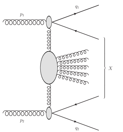
Figure 1: Diagrammatic representation of the heavy-quark pair hadroproduction in the case when a heavy quark with transverse momentum $q_{1}(q_{2})$ from the upper (lower) vertex is tagged.

2 Theoretical setup

For the process under consideration (see Fig. 1) we plan to construct the cross section, differential in some of the kinematic variables of the tagged heavy quark or antiquark, and some azimuthal correlations between the tagged fermions. In the BFKL approach the cross section takes the factorized form, diagrammatically represented in Fig. 2, given by the convolution of the impact factors for the transition from a real gluon to a heavy quark-antiquark pair with the BFKL Green’s function $G$.

In our calculation we will partially include NLA resummation effects, by taking the BFKL Green’s function in the NLA, while the impact factors are kept at leading order.

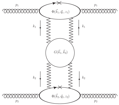
Figure 2: Schematic representation of the BFKL factorization for the heavy-quark pair hadroproduction.

2.1 Impact factor

The (differential) impact factor for the hadroproduction of a heavy-quark pair reads 

$$\begin{split}d\Phi^{\{{Q\bar{Q}\}}}_{gg}(\vec{k},\vec{q},z)&=\frac{\alpha_{s}^{2}\sqrt{N_{c}^{2}-1}}{2\pi N_{c}}\left[\left(m^{2}\left(R+\bar{R}\right)^{2}+\left(z^{2}+\bar{z}^{2}\right)\left(\vec{P}+\vec{\bar{P}}\right)^{2}\right)\right.\\ &\left.-\frac{N_{c}^{2}}{N_{c}^{2}-1}\left(2m^{2}R\bar{R}+\left(z^{2}+\bar{z}^{2}\right)2\vec{P}\cdot\vec{\bar{P}}\right)\right]\;d^{2}\vec{q}\;dz\;,\end{split}$$ (2)

where $R$, $\bar{R}$, $\vec{P}$ and $\vec{\bar{P}}$ are defined as

$$R=\frac{1}{m^{2}+\vec{q}^{\;2}}-\frac{1}{m^{2}+(\vec{q}-z\vec{k})^{2}}\;,$$ (3)

$$\bar{R}=\frac{1}{m^{2}+(\vec{q}-z\vec{k})^{2}}-\frac{1}{m^{2}+(\vec{q}-\vec{k})^{2}}\;,$$ (4)

$$\vec{P}=\frac{\vec{q}}{m^{2}+\vec{q}^{\;2}}-\frac{\vec{q}-z\vec{k}}{m^{2}+(\vec{q}-z\vec{k})^{2}}\;,$$ (5)

$$\vec{\bar{P}}=\frac{\vec{q}-z\vec{k}}{m^{2}+(\vec{q}-z\vec{k})^{2}}-\frac{\vec{q}-\vec{k}}{m^{2}+(\vec{q}-\vec{k})^{2}}\;.$$ (6)

Here $\alpha_{s}$ denotes the QCD coupling, $N_{c}$ gives the number of colors, $m$ stands for the heavy-quark mass, $z$ and $\bar{z}\equiv 1-z$ are the longitudinal momentum fractions of the quark and antiquark produced in the same vertex and $k$, $q$, $k-q$ represent the transverse momenta with respect to the gluons collision axis of the Reggeized gluon, the produced quark and antiquark, respectively.

In the following we will need the projection of the impact factors onto the eigenfunctions of the leading-order BFKL kernel, to get their so called $(n,\nu)$-representation. We get

$$\frac{d\Phi_{gg}^{\{{Q\bar{Q}\}}}\left(n,\nu,\vec{q},z\right)}{d^{2}\vec{q}\;dz}\equiv\int\frac{d^{2}\vec{k}}{\pi\sqrt{2}}(\vec{k}^{\;2})^{i\nu-\frac{3}{2}}e^{in\theta}\frac{d\Phi^{\{{Q\bar{Q}\}}}_{gg}(\vec{k},\vec{q},z)}{d^{2}\vec{q}\;dz}$$

$$=\frac{\alpha_{s}^{2}\sqrt{N_{c}^{2}-1}}{2\pi N_{c}}\left\{m^{2}\left(I_{3}-2\frac{I_{2}(0)}{m^{2}+\vec{q}^{\;2}}\right)+(z^{2}+\bar{z}^{2})\left(-m^{2}\left(I_{3}-2\frac{I_{2}(0)}{m^{2}+\vec{q}^{\;2}}\right)+\frac{I_{2}(1)}{m^{2}+\vec{q}^{\;2}}\right)\right.$$

$$\left.-\frac{N_{c}^{2}}{N_{c}^{2}-1}\Bigg{[}2m^{2}\left[\left(z^{2}+\bar{z}^{2}-1\right)\left(1-\left(z^{2}\right)^{\frac{1}{2}-i\nu}\right)\right]\frac{I_{2}(0)}{m^{2}+\vec{q}^{\;2}}+\left[2m^{2}(z^{2}+\bar{z}^{2}-1)\left(z^{2}\right)^{\frac{1}{2}-i\nu}\right]\right.$$

$$\left.\left(I_{3}-\frac{I_{4}(0)}{\left(z^{2}\right)^{\frac{1}{2}-i\nu}}\right)-(z^{2}+\bar{z}^{2})\bigg{[}(1-z)^{2}I_{4}(1)-\frac{\left(1-\left(z^{2}\right)^{\frac{1}{2}-i\nu}\right)}{m^{2}+\vec{q}^{\;2}}I_{2}(1)\bigg{]}\Bigg{]}\right\}$$

$$\equiv\alpha_{s}^{2}\;e^{in\varphi}c(n,\nu,\vec{q},z)\;,$$ (7)

where $I_{2}(\lambda)$, $I_{3}$ and $I_{4}(\lambda)$ read

$$\begin{split}I_{2}\left(\lambda\right)&=\frac{\left(\vec{q}^{\;2}\right)^{\frac{n}{2}}e^{in\varphi}}{\sqrt{2}}\frac{1}{\left(m^{2}+\vec{q}^{\;2}\right)^{\frac{3}{2}+\frac{n}{2}-i\nu-\lambda}}\frac{\Gamma\left(\frac{1}{2}+\frac{n}{2}+i\nu+\lambda\right)\Gamma\left(\frac{1}{2}+\frac{n}{2}-i\nu-\lambda\right)}{\Gamma\left(1+n\right)}\\ &\times\frac{\left(\frac{1}{2}+\frac{n}{2}-i\nu-\lambda\right)}{\left(-\frac{1}{2}+\frac{n}{2}+i\nu+\lambda\right)}\;_{2}F_{1}\left(-\frac{1}{2}+\frac{n}{2}+i\nu+\lambda,\frac{3}{2}+\frac{n}{2}-i\nu-\lambda,1+n,\zeta\right)\;,\end{split}$$ (8)

$$\begin{split}I_{3}=\frac{\left(\vec{q}^{\;2}\right)^{\frac{n}{2}}e^{in\varphi}}{\sqrt{2}}&\frac{1}{\left(m^{2}+\vec{q}^{\;2}\right)^{\frac{5}{2}+\frac{n}{2}-i\nu}}\frac{\Gamma\left(\frac{1}{2}+\frac{n}{2}+i\nu\right)\Gamma\left(\frac{1}{2}+\frac{n}{2}-i\nu\right)}{\Gamma\left(1+n\right)}\frac{\left(\frac{1}{2}+\frac{n}{2}-i\nu\right)}{\left(-\frac{1}{2}+\frac{n}{2}+i\nu\right)}\;\\ &\times\left(\frac{3}{2}+\frac{n}{2}-i\nu\right)\;_{2}F_{1}\left(-\frac{1}{2}+\frac{n}{2}+i\nu,\frac{5}{2}+\frac{n}{2}-i\nu,1+n,\zeta\right)\;,\end{split}$$ (9)

$$\begin{split}I_{4}\left(\lambda\right)=&\frac{\left(\vec{q}^{\;2}\right)^{\frac{n}{2}}e^{in\varphi}}{z^{2}\sqrt{2}}\frac{\left(\frac{3}{2}-i\nu-\lambda+\frac{n}{2}\right)}{\left(m^{2}+\vec{q}^{\;2}\right)^{\frac{5}{2}-i\nu-\lambda+\frac{n}{2}}}\frac{\Gamma\left(\frac{1}{2}+\frac{n}{2}+i\nu+\lambda\right)\Gamma\left(\frac{1}{2}+\frac{n}{2}-i\nu-\lambda\right)}{\Gamma\left(1+n\right)}\\ &\times\frac{\left(\frac{1}{2}+\frac{n}{2}-i\nu-\lambda\right)}{\left(-\frac{1}{2}+\frac{n}{2}+i\nu+\lambda\right)}\int_{0}^{1}d\Delta\left(1+\frac{\Delta}{z}-\Delta\right)^{n}\left(1+\frac{\Delta}{z^{2}}-\Delta\right)^{-\frac{5}{2}+i\nu+\lambda-\frac{n}{2}}\;\\ &\times\;_{2}F_{1}\left(-\frac{1}{2}+i\nu+\lambda+\frac{n}{2},\frac{5}{2}-i\nu-\lambda+\frac{n}{2},1+n,\zeta\;\frac{\left(1+\frac{\Delta}{z}-\Delta\right)^{2}}{\left(1+\frac{\Delta}{z^{2}}-\Delta\right)}\right)\;,\end{split}$$ (10)

and $\zeta\equiv\frac{\vec{q}^{\;2}}{m^{2}+\vec{q}^{\;2}}$; the azimuthal angles $\theta$ and $\varphi$ are defined as $\cos\theta\equiv k_{x}/|\vec{k}|$ and $\cos\varphi\equiv q_{x}/|\vec{q}|$. We refer the reader to the Appendix B for details on the derivation of these results.

2.2 Kinematics of the process

For the tagged quark momenta we introduce the standard Sudakov decomposition, using as light-cone basis the momenta $p_{1}$ and $p_{2}$ of the colliding gluons,

$$q=zp_{1}+\frac{m^{2}+\vec{q}^{\;2}}{zW^{2}}p_{2}+q_{\perp}\;,$$ (11)

with $W^{2}=(p_{1}+p_{2})^{2}=2p_{1}\cdot p_{2}=4E_{g_{1}}E_{g_{2}}$ ; $p_{1}=E_{g_{1}}(1,\vec{0},1)$ and $p_{2}=E_{g_{2}}(1,\vec{0},-1)$, so that

$$2q\cdot p_{2}=2zp_{1}\cdot p_{2}=zW^{2}=2E_{g_{2}}\left(E+q_{\|}\right)\;,$$ (12)

$$2q\cdot p_{1}=\frac{m^{2}+\vec{q}^{\;2}}{z}=2E_{g_{1}}\left(E-q_{\|}\right)\;;$$ (13)

here $q=(E,\vec{q},q_{\|})$ and the rapidity can be expressed as

$$y=\frac{1}{2}\ln\frac{\left(E+q_{\|}\right)}{\left(E-q_{\|}\right)}=\ln\left[\frac{2zE_{g_{1}}}{\sqrt{m^{2}+\vec{q}^{\;2}}}\right]\;.$$ (14)

Accordingly, the rapidities of the two tagged quarks in our process are

$$y_{1}=\ln\left[\frac{2z_{1}E_{g_{1}}}{\sqrt{m^{2}+\vec{q}_{1}^{\;2}}}\right]\hskip 5.69046pt{\rm{and}}\hskip 5.69046pty_{2}=-\ln\left[\frac{2z_{2}E_{g_{2}}}{\sqrt{m^{2}+\vec{q}_{2}^{\;2}}}\right]\;,$$ (15)

whence their rapidity difference is

$$\Delta Y\equiv y_{1}-y_{2}=\ln\frac{W^{2}z_{1}z_{2}}{\sqrt{\left(m^{2}+\vec{q}_{1}^{\;2}\right)\left(m^{2}+\vec{q}_{2}^{\;2}\right)}}\;.$$ (16)

For the semi-hard kinematics we have the requirement

$$\frac{W^{2}}{\sqrt{\left(m^{2}+\vec{q}_{1}^{\;2}\right)\left(m^{2}+\vec{q}_{2}^{\;2}\right)}}=\frac{e^{\Delta Y}}{z_{1}z_{2}}\gg 1\;,$$ (17)

therefore we will consider the kinematics when $\Delta Y\geq\Delta_{0}\sim 1\div 2$.

In what follows, we will need a cross section differential in the rapidities of the tagged quarks. For this reason we adopt the change of variables:

$$z_{1}\to y_{1}=\ln\left[\frac{2z_{1}E_{g_{1}}}{\sqrt{m^{2}+\vec{q}_{1}^{\;2}}}\right]\;,\quad dy_{1}=\frac{dz_{1}}{z_{1}}\;,$$

$$z_{2}\to y_{2}=-\ln\left[\frac{2z_{2}E_{g_{2}}}{\sqrt{m^{2}+\vec{q}_{2}^{\;2}}}\right]\;,\quad dy_{2}=-\frac{dz_{2}}{z_{2}}\;,$$

which implies

$$dz_{1}dz_{2}=\frac{e^{\Delta Y}\sqrt{m^{2}+\vec{q}_{1}^{\;2}}\sqrt{m^{2}+\vec{q}_{2}^{\;2}}}{W^{2}}dy_{1}dy_{2}\;.$$

2.3 The BFKL cross section and azimuthal coefficients

The differential cross section for the inclusive production of a pair of heavy quarks separated in rapidity can be cast in the form:

$$\frac{d\sigma_{gg}}{dy_{1}dy_{2}d|\vec{q}_{1}|d|\vec{q}_{2}|d\varphi_{1}d\varphi_{2}}=\frac{1}{(2\pi)^{2}}\left[\mathcal{C}_{0}+2\sum_{n=1}^{\infty}\cos(n\varphi)\mathcal{C}_{n}\right],$$ (18)

where $\varphi=\varphi_{1}-\varphi_{2}-\pi$, while $\mathcal{C}_{0}$ gives the, $\varphi$-averaged, cross section summed over the azimuthal angles, $\varphi_{1,2}$, of the produced quarks, and the other coefficients, $\mathcal{C}_{n}$, determine the distribution of the relative azimuthal angle between the two quarks.

The expression for the $\mathcal{C}_{n}$ coefficient is the following (see, e.g., Ref. [38]):

$$\begin{split}\mathcal{C}_{n}=&\frac{|\vec{q}_{1}||\vec{q}_{2}|\sqrt{m^{2}+\vec{q}_{1}^{\;2}}\sqrt{m_{2}^{2}+\vec{q}_{2}^{\;2}}}{W^{2}}e^{\Delta Y}\\ &\times\int_{-\infty}^{+\infty}d\nu\left(\frac{W^{2}}{s_{0}}\right)^{\bar{\alpha}_{s}\left(\mu_{R}\right)\chi\left(n,\nu\right)+\bar{\alpha}_{s}^{2}\left(\mu_{R}\right)\left(\bar{\chi}\left(n,\nu\right)+\frac{\beta_{0}}{8N_{c}}\chi\left(n,\nu\right)\left(-\chi\left(n,\nu\right)+\frac{10}{3}+2\ln\frac{\mu_{R}^{2}}{\sqrt{s_{1}s_{2}}}\right)\right)}\\ &\times\alpha_{s}^{4}\left(\mu_{R}\right)c_{1}\left(n,\nu,\vec{q}_{1}^{\;2},z_{1}\right)c_{2}\left(n,\nu,\vec{q}_{2}^{\;2},z_{2}\right)\left\{1+\bar{\alpha}_{s}\left(\mu_{R}\right)\left(\frac{\bar{c}_{1}^{(1)}}{c_{1}}+\frac{\bar{c}_{2}^{(1)}}{c_{2}}\right)\right.\\ &\left.+\bar{\alpha}_{s}\left(\mu_{R}\right)\frac{\beta_{0}}{2N_{c}}\left(\frac{5}{3}+\ln\frac{\mu_{R}^{2}}{s_{1}s_{2}}+f\left(\nu\right)\right)+\bar{\alpha}_{s}^{2}\left(\mu_{R}\right)\ln\left(\frac{W^{2}}{s_{0}}\right)\frac{\beta_{0}}{4N_{c}}\chi\left(n,\nu\right)f\left(\nu\right)\right\}\;,\end{split}$$ (19)

where

$$\chi\left(n,\nu\right)=2\psi(1)-\psi\left(\frac{n}{2}+\frac{1}{2}+i\nu\right)-\psi\left(\frac{n}{2}+\frac{1}{2}-i\nu\right)$$ (20)

are the eigenvalues of the leading-order BFKL kernel, with $\psi=\Gamma^{\prime}(x)/\Gamma(x)$, and

$$\beta_{0}=\frac{11}{3}N_{c}-\frac{2}{3}n_{f}$$ (21)

is the first coefficient of the QCD $\beta$-function, responsible for running-coupling effects. The function $f\left(\nu\right)$ is defined by

$$i\frac{d}{d\nu}\ln\frac{c_{1}}{c_{2}}=2\left[f(\nu)-\ln(\sqrt{s_{1}s_{2}})\right]\;,$$ (22)

with $s_{i}$, $i=1,2$ the hard scales in our two-tagged-quark process, which are chosen to be equal to $m_{i}^{2}+\vec{q}_{i}^{\;2}$, and

$$\begin{split}c_{1}\left(n,\nu,\vec{q}_{1}^{\;2},z_{1}\right)=\frac{1}{e^{in\varphi_{1}}\alpha_{s}^{2}}\frac{d\Phi_{gg}^{\{{Q\bar{Q}\}}}\left(n,\nu,\vec{q}_{1},z_{1}\right)}{d^{2}\vec{q}_{1}\;dz_{1}}\end{split}$$ (23)

$$\begin{split}c_{2}\left(n,\nu,\vec{q}_{2}^{\;2},z_{2}\right)=\frac{1}{e^{-in(\varphi_{2}+\pi)}\alpha_{s}^{2}}\left[\frac{d\Phi_{gg}^{\{{Q\bar{Q}\}}}\left(n,\nu,\vec{q}_{2},z_{2}\right)}{d^{2}\vec{q}_{2}\;dz_{2}}\right]^{*}\end{split}$$ (24)

$$\frac{\bar{c}_{1}^{(1)}}{c_{1}}+\frac{\bar{c}_{2}^{(1)}}{c_{2}}=\chi\left(n,\nu\right)\ln\frac{s_{0}}{\sqrt{\left(m_{1}^{2}+\vec{q}_{1}^{\;2}\right)\left(m_{2}^{2}+\vec{q}_{2}^{\;2}\right)}}\;.$$ (25)

The presence in the latter formula of the combination $\varphi_{2}+\pi$ is due to the fact that, in the second impact factor, the Reggeon is outgoing instead of incoming. The scale $s_{0}$ can be arbitrarily chosen, within NLA accuracy; in this calculation, the choice $s_{0}=\sqrt{s_{1}s_{2}}$ has been made. It is worth to remark that Eq. (19) is written for the general case when two heavy quarks of different masses $m_{1},m_{2}$ are detected.

2.4 The proton-proton cross section

In order to pass from the gluon-initiated process to the one initiated by proton-proton collisions, we must take into account the distribution of the gluons inside the two colliding particles,

$$d\sigma_{pp}=f_{g_{1}}(x_{1},\mu_{F_{1}})f_{g_{2}}(x_{2},\mu_{F_{2}})d\sigma_{gg}dx_{1}dx_{2}\;,$$ (26)

with $f_{g_{i}}$, $i=1,2$ being the gluon collinear parton distribution functions and $d\sigma_{gg}$ the cross-section in Eq. (27). Therefore the final expression for our observable is

$$\frac{d\sigma_{pp}}{d(\Delta Y)d\varphi_{1}d\varphi_{2}}=\frac{1}{(2\pi)^{2}}\left[C_{0}+2\sum_{n=1}^{\infty}\cos(n\varphi)C_{n}\right]\;,$$ (27)

where

$$\begin{split}C_{n}=&\int_{q_{1,{\rm{min}}}}^{q_{1,{\rm{max}}}}d|\vec{q}_{1}|\int_{q_{2,{\rm{min}}}}^{q_{2,{\rm{max}}}}d|\vec{q}_{2}|\int_{y_{1,{\rm{min}}}}^{y_{1,{\rm{max}}}}dy_{1}\int_{y_{2,{\rm{min}}}}^{y_{2,{\rm{max}}}}dy_{2}\;\delta(y_{1}-y_{2}-\Delta Y)\\ &\int_{e^{-(y_{1,{\rm{max}}}-y_{1})}}^{1}dx_{1}f_{g_{1}}(x_{1},\mu_{F_{1}})\int_{e^{-(y_{2,{\rm{max}}}+y_{2})}}^{1}dx_{2}f_{g_{2}}(x_{2},\mu_{F_{2}})\;\mathcal{C}_{n}\end{split}$$ (28)

stands for the $n^{\rm th}$ azimuthal coefficient integrated over the $(\vec{q}_{1,2},y_{1,2})$ phase space and the rapidity separation between the two tagged quarks is kept fixed to $\Delta Y$.

2.5 The “box” $Q\bar{Q}$ cross section

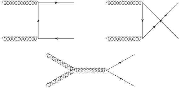
Figure 3: Feynman diagrams contributing at the lowest order to the $Q\bar{Q}$ hadroproduction.

In this section, we consider, for the sake of comparison, the lowest-order QCD cross section for the production of a heavy quark-antiquark pair in proton-proton collisions. This process, which we dub “box” with a little abuse of terminology, does not represent a background for the inclusive reaction of interest in this work when the two detected heavy quarks are of different flavors or, being of the same flavors, are both quark or both antiquarks.

The Feynman diagrams contributing to this process at the leading order are shown in Fig. 3. The differential cross section is presented, e.g., in Ref. [68] and in our notation takes the form

$$\begin{split}\frac{d\sigma_{pp}}{d(\Delta Y)}=\;&\frac{\pi\alpha_{s}^{2}}{s(N_{c}^{2}-1)}\int_{{\rm min}(q^{2}_{\rm min},\frac{s}{4\cosh^{2}(\Delta Y/2)}-m^{2})}^{{\rm min}(q^{2}_{\rm max},\frac{s}{4\cosh^{2}(\Delta Y/2)}-m^{2})}\frac{d\vec{q}^{\>2}}{M^{2}}\int_{\frac{M^{2}}{s}}^{1}\frac{dx}{x}f_{g_{1}}(x,\mu_{F_{1}})f_{g_{2}}(M^{2}/xs,\mu_{F_{2}})\\ &\times\left(C_{F}\frac{M^{4}}{t_{1}u_{1}}-C_{A}\right)\left[\frac{t_{1}^{2}+u_{1}^{2}}{M^{4}}+4\frac{m^{2}}{M^{2}}-4\frac{m^{4}}{t_{1}u_{1}}\right]\;,\end{split}$$ (29)

where

$$M^{2}=4(m^{2}+\vec{q}^{\>2})\cosh^{2}(\Delta Y/2)\;,$$ (30)

$$t_{1}=-\frac{M^{2}}{2}\left[1-\tanh(\Delta Y/2)\right]\;,$$ (31)

$$u_{1}=-\frac{M^{2}}{2}\left[1+\tanh(\Delta Y/2)\right]\;.$$ (32)

Here, $C_{F}=(N_{c}^{2}-1)/2N_{c}$, $C_{A}=N_{c}$, $s$ is the squared center-of-mass energy of the proton-proton system and $m$ is the heavy-quark mass; $\mu_{F_{1}}$, $\mu_{F_{2}}$ are both set to $\sqrt{m_{Q}^{2}+\vec{q}^{\>2}}$ and $\alpha_{s}$ is also calculated at this scale. The upper and lower limits in the integration over $\vec{q}^{\>2}$ come from the constraint $M^{2}\leq s$; in their expression, $q^{2}_{\rm min}$ and $q^{2}_{\rm max}$ represent the kinematic cuts on the heavy quark/antiquark transverse momentum. There is also a constraint on $\Delta Y$, coming from the requirement that $M^{2}|_{\vec{q}^{\>2}=0}\leq s$, which is however always fulfilled for the values of $\Delta Y$ and $s$ considered in the numerical analysis presented below.

3 Numerical analysis

3.1 Results

In this Section we present our results for the dependence on the rapidity interval between the two tagged bottom quarks, $\Delta Y\equiv y_{1}-y_{2}$, of the $\varphi$-averaged cross section $C_{0}$ and of the azimuthal correlations, $R_{n0}=C_{n}/C_{0}\equiv\langle\cos n\varphi\rangle$, and their ratios, $R_{n0}=C_{n}/C_{m}$ [71, 72]. We fix the $m_{1,2}$ masses at the value $m_{b}=4.18$ GeV/$c^{2}$ [73].

With the idea of matching realistic kinematic configurations, typical of the current and possible future LHC analyses, we integrate the quark transverse momenta in the symmetric range 20 GeV $<q_{1,2}<$ 100 GeV, fixing the center-of-mass energy to $\sqrt{s}=14$ TeV and studying the behavior of our observables in the rapidity range $1.5<\Delta Y<9$. Ranges of the transverse momenta of the bottom-jets ($b$-jets) are typical of CMS analyses [74, 75].

Pure LLA and NLA BFKL predictions for the $\varphi$-averaged cross section, $C_{0}$, together with the leading-order $pp\rightarrow q\bar{q}$ cross section, are presented in Table 1. Results for $C_{0}$ and for several azimuthal-correlation ratios, $R_{nm}$, are shown in Fig. 4.

As a complementary study (see Fig. 5), we present results for $C_{0}$ in the case of charmed-jet ($c$-jet) pair emission ($m_{1,2}=m_{c}=1.2$ GeV/$c^{2}$), comparing predictions for the hadroproduction with the ones related to the photoproduction mechanism (see Ref. [66] for details on the theoretical framework and for a recent phenomenological analysis conducted by some of us) in the kinematic configurations typical of the future CLIC linear accelerator, namely 1 GeV $<q_{1,2}<$ 10 GeV, $\sqrt{s}=3$ TeV and $1.5<\Delta Y<10.5$.

All calculations are done in the $\overline{\rm MS}$ scheme.

Table 1: $\Delta Y$-dependence of the $\varphi$-averaged cross section $C_{0}$ [nb] for $\sqrt{s}=14$ TeV. $C_{\mu}$ stands for $\mu_{R}^{2}/\sqrt{s_{1}s_{2}}\equiv\mu_{F_{1,2}}^{2}/s_{1,2}$.

$\Delta Y$	$\begin{array}[]{c}\rm Box\\ Q\bar{Q}\end{array}$	$\begin{array}[]{c}\rm LLA\\ C_{\mu}=1/2\end{array}$	$\begin{array}[]{c}\rm LLA\\ C_{\mu}=1\end{array}$	$\begin{array}[]{c}\rm LLA\\ C_{\mu}=2\end{array}$	$\begin{array}[]{c}\rm NLA\\ C_{\mu}=1/2\end{array}$	$\begin{array}[]{c}\rm NLA\\ C_{\mu}=1\end{array}$	$\begin{array}[]{c}\rm NLA\\ C_{\mu}=2\end{array}$
1.5	33830.3	38.17(24)	30.01(21)	23.58(16)	22.25(26)	23.93(23)	25.19(27)
3.0	3368.86	18.118(98)	13.191(71)	9.838(61)	7.245(74)	8.205(76)	8.172(82)
4.5	124.333	6.996(33)	4.715(23)	3.276(16)	2.209(20)	2.411(17)	2.422(19)
6.0	3.19206	1.976(10)	1.2430(60)	0.8044(38)	0.4497(35)	0.4968(35)	0.4868(37)
7.5	0.0610921	0.3317(16)	0.19115(92)	0.11509(57)	0.05318(36)	0.05785(39)	0.05577(42)
9.0	0.000681608	0.02215(10)	0.011458(56)	0.006340(30)	0.002566(17)	0.002668(16)	0.002513(16)

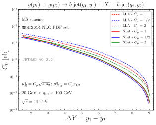
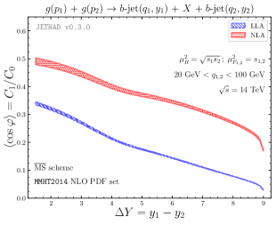
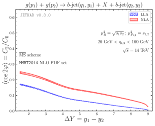
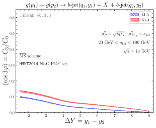
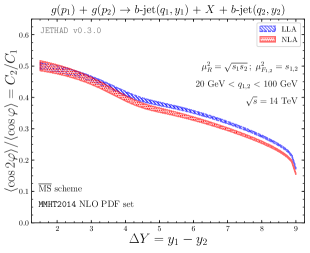
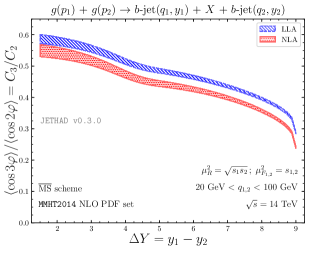
Figure 4: $\Delta Y$-dependence of $C_{0}$ ($b$-jet pair) for different values of $C_{\mu}=\mu_{R}^{2}/\sqrt{s_{1}s_{2}}\equiv\mu^{2}_{F_{1,2}}/s_{1,2}$ (data points have been slightly shifted along the horizontal axis for the sake of readability), with $s_{1,2}=m^{2}_{1,2}+\vec{q}_{1,2}^{\;2}$ and of several ratios $R_{nm}\equiv C_{n}/C_{m}$, for 20 GeV $<q_{1,2}<$ 100 GeV and $\sqrt{s}=14$ TeV.

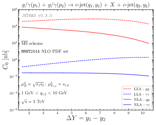
Figure 5: $\Delta Y$-dependence of $C_{0}$ ($c$-jet pair) for both the hadroproduction ($gg$) and the photoproduction ($\gamma\gamma$) mechanisms, for 1 GeV $<q_{1,2}<$ 10 GeV and $\sqrt{s}=3$ TeV.

3.2 Numerical strategy and uncertainty estimate

The numerical analysis was done using Jethad, a Fortran code we recently developed, oriented towards the study of inclusive semi-hard processes. In order to perform numerical integrations, Jethad was interfaced with the Cern program library [76] and with the Cuba integrators [77, 78], making extensive use of the Vegas [79] and the WGauss [76] integrators. The numerical stability of our predictions was crosschecked using an independent Mathematica code. The gluon PDFs ($f_{g_{1,2}}$) were calculated via the MMHT2014 NLO PDF parameterization [80] as implemented in the Les Houches Accord PDF Interface (LHAPDF) 6.2.1 [81], while a two-loop running coupling setup with $\alpha_{s}\left(M_{Z}\right)=0.11707$ with dynamic-flavor thresholds was chosen.

The most relevant source of uncertainty, coming from the numerical six-dimensional integration over the variables $|\vec{q}_{1}|$, $|\vec{q}_{2}|$, $y_{1}$, $\nu$, $x_{1}$, and $x_{2}$, was directly estimated by Vegas. Other sources of uncertainties, related with the upper cutoff in the $\nu$- and the $\Delta$-integration in Eq. (19) and Eq. (10), respectively, are negligible with respect to the first one. Thus, the error estimates of our predictions are just those given by Vegas. In order to quantify the uncertainty related to the renormalization scale ($\mu_{R}$) and the factorization one ($\mu_{F_{1,2}}$), we simultaneously vary the square of both of them around their “natural” values, $\sqrt{s_{1}s_{2}}$ and $s_{1,2}$ respectively, in the range 1/2 to two. The parameter $C_{\mu}$ entering Table 1 gives the ratio $C_{\mu}=\mu_{R}^{2}/\sqrt{s_{1}s_{2}}\equiv\mu_{F_{1,2}}^{2}/s_{1,2}$.

3.3 Discussion

The inspection of results for the $\varphi$-averaged cross section, $C_{0}$, in the $b$-jet pair production case (Table 1 and in the left upper panel of Fig. 4) clearly indicates the usual onset of the BFKL dynamics. On the one hand, although the high-energy resummation predicts a growth with energy of the partonic-subprocess cross section, its convolution with parent-gluon PDFs (Eq. (26)) leads, as a net effect, to a falloff with $\Delta Y$ of both LLA and NLA predictions. On the other hand, next-to-leading corrections to the BFKL kernel become more and more negative when the rapidity distance grows, thus making NLA results steadily lower than pure LLA ones.

Data in Table 1 also show that the cross section $C_{0}$ is smaller than the reference “box” cross section for small $\Delta Y$; at larger rapidity differences, however, the BFKL mechanism with the gluonic exchange in the $t$-channel starts to dominate. We stress, however, that for our two heavy-quark (or two heavy-antiquark) tagged process, the “box” mechanism is not a background.

Azimuthal correlations (remaining panels of Fig. 4) are always smaller than one and decrease when $\Delta Y$ grows (LLA results are always more decorrelated than NLA ones), as an expected consequence of the larger emission of undetected partons (the $X$ system in Eq. (3)). The cause for this narrowness, with respect to other, recently investigated reactions, such as Mueller–Navelet jet, dihadron or hadron-jet correlations (see, e.g., Refs. [31, 47, 58]), is straightforward. Since the two detected (anti)quarks stem from distinct vertices (each of them together the respective antiparticle), their transverse momenta are kinematically not constrained at all, even at leading order.

The analysis presented in Fig. 5 for the $c$-jet pair production unambiguously shows that, at fixed center-of-mass energy and transverse-momentum range, predictions for $C_{0}$ in the hadroproduction channel ($gg$) are several orders of magnitude higher than the corresponding ones in the photoproduction case ($\gamma\gamma$). This comes as a result of two competing effects. On one side, from a “rough” comparison between the ($gg$) impact factor (Eq. (2)) and the ($\gamma\gamma$) one (Eq. (2) of Ref. [66] and footnote of Ref. [67]), it emerges that the two analytic structures are quite similar, the main difference being the fact that, since the photon cannot interact directly with the Reggeized gluon, some terms present in the first case are missing in the second one. In both of the two impact factors there are constants that can be factorized out in the final form of the cross section. Since two heavy-quark impact factors enter the expression of cross sections, one has an overall factor

$$\kappa_{(gg)}=\frac{\alpha_{s}^{4}\,(N_{c}^{2}-1)}{(2\pi N_{c})^{2}}$$ (33)

in the ($gg$) case and an overall factor

$$\kappa_{(\gamma\gamma)}=\frac{\alpha_{\rm em}^{2}\,\alpha_{s}^{2}\,e_{c}^{4}(N_{c}^{2}-1)}{\pi^{2}}$$ (34)

in the ($\gamma\gamma$) case, with $\alpha_{\rm em}$ the QED coupling and $e_{c}$ the electric charge of the charm quark in units of the positron charge. The ratio between the two factors is

$$\kappa_{{}^{(gg)}\!/_{(\gamma\gamma)}}\equiv\frac{\kappa_{(gg)}}{\kappa_{(\gamma\gamma)}}\simeq 3\div 4\times 10^{3}\;,$$ (35)

which would explain the enhancement of the hadroproduction with respect to the photoproduction. On the other side, however, one should take into account the effect of the parent-particle distributions: gluon PDF [80] or EPA photon flux (see Eq. (8) of Ref. [66]). It is possible to show that the gluon PDF dominates over the photon flux in the moderate-$x$ region, while the second one prevails in the $x\to 0^{+}$ and $x\to 1^{-}$ limits. In the realistic kinematic ranges we have considered in this paper and in Refs. [66, 67] the relevant $x$-region turns to be just the intermediate one, thus leading to an enhancement of the hadroproduction mechanism with respect to the photoproduction one (see, e.g., Fig. 5) even larger than what suggested by the ratio $\kappa_{{}^{(gg)}\!/_{(\gamma\gamma)}}$.

4 Summary and outlook

We have proposed the inclusive hadroproduction of two heavy quarks separated by a large rapidity interval as a new channel for the investigation of BFKL dynamics. We have performed an all-order resummation of the leading energy logarithms and a resummation of the next-to-leading ones entering the BFKL Green’s function. In this approximation, the cross section can be written as the convolution of the partonic cross section for the collision of two gluons producing the two heavy quarks with the respective gluon PDFs.

We have calculated the cross section for this process summed over the relative azimuthal angle of the two tagged quarks and presented results for the azimuthal angle correlations. The behavior of these observables turned to be the usual one, characteristic feature of the onset of the BFKL dynamics. Finally, a comparison between the photoproduction and the hadroproduction mechanism has been carried out.

This process enriches the selection of semi-hard reactions that can be used as probes of the QCD in the high-energy limit, and in particular of the BFKL resummation mechanism, in the kinematic ranges of the LHC and of future hadronic colliders.

Several prospective developments of this work can be planned and afforded. The first one consists in the calculation of the NLO correction to the forward heavy-quark pair impact factor, which would allow for a full NLA BFKL treatment of the process under consideration. The second one is to include into the theoretical analysis the quark fragmentation needed to match, from the theoretical side, the experimental tagging procedure of heavy-quark mesons. Since the photoproduction channel has already been considered (Refs. [66, 67]), a process of photo/hadro-production (when the first (anti)quark is emitted by a (quasi-)real photon, while the second one stems from a gluon), hybrid with respect to the previous ones, can also be examined. One last idea is to investigate semi-hard channels featuring the emission of a single quark. For instance, one can study the single forward heavy-quark production, convolving the corresponding impact factor with the unintegrated gluon density (UGD) in the proton.

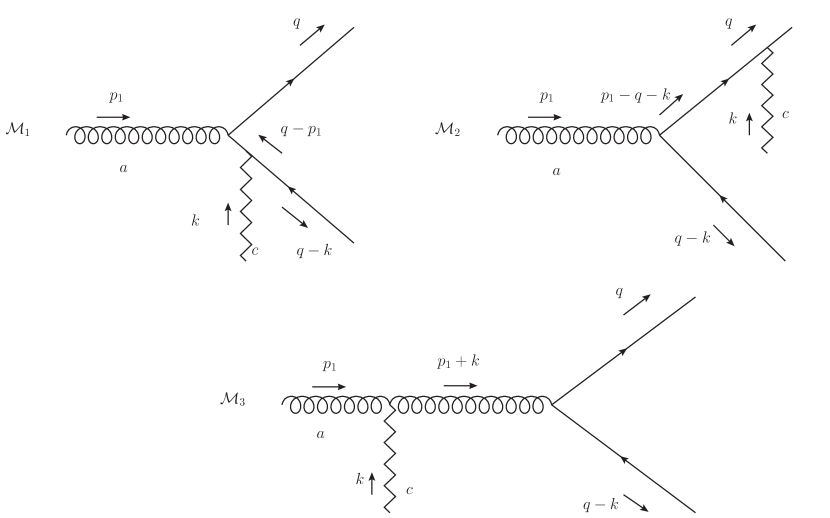
Figure 6: Feynman diagrams relevant for the calculation of the impact factor for the heavy-quark pair hadroproduction. The zigzag line denotes a Reggeized gluon.

Appendix A

In this Section we give the expression of the leading-order impact factor, together with the functional form of the amplitude for the $g+R\to q\bar{q}$ subprocess, where $R$ here means “Reggeized gluon”. The leading-order impact factor is defined as [69]

$$\begin{split}d\Phi_{gg}^{\{{Q\bar{Q}\}}}(\vec{q},\vec{k},z)=&\frac{\braket{cc^{\prime}}{\mathcal{\widehat{P}}}{0}}{2\left(N^{2}-1\right)}\\ &\times\sum_{\lambda_{Q}\lambda_{\bar{Q}}\lambda_{G}}\sum_{Q\bar{Q}a}\int\frac{ds_{gR}}{2\pi}d\rho_{\{{Q\bar{Q}\}}}\Gamma_{g\rightarrow\{{Q\bar{Q}\}}}^{ca}\left(q,k,z\right)\left(\Gamma_{g\rightarrow\{{Q\bar{Q}\}}}^{ac^{\prime}}\left(q,k,z\right)\right)^{\ast}\;,\end{split}$$ (36)

where

$$\braket{cc^{\prime}}{\mathcal{\widehat{P}}}{0}=\frac{\delta^{cc^{\prime}}}{\sqrt{N^{2}-1}}$$ (37)

is the projector on the singlet state. We take the sum over helicities, $\{\lambda_{Q},\lambda_{\bar{Q}}\}$, and over color indices, $\{Q,\bar{Q}\}$, of the two produced particles (quark and antiquark) and average over polarization and color states of the incoming gluon. In Eq. (36), $s_{gR}$ denotes the invariant squared mass of the gluon-Reggeon system, while $d\rho_{\{{Q\bar{Q}\}}}$ is the differential phase space of the outgoing particles. The amplitude $\Gamma_{g\rightarrow\{{Q\bar{Q}\}}}^{ca}$ describes the production of quark-antiquark pair in a collision between a gluon and a Reggeon. The latter can be treated as an ordinary gluon in the so called “nonsense” polarization state $\epsilon_{R}^{\mu}=p_{2}^{\mu}/s$, see, e.g., Ref. [70]. Having two particles produced in the intermediate state, one can write

$$\frac{ds_{gR}}{2\pi}d\rho_{\{{Q\bar{Q}\}}}=\frac{1}{2\left(2\pi\right)^{3}}\delta\left(1-z-\bar{z}\right)\delta^{(2)}\left(\vec{k}-\vec{q}-\vec{\bar{q}}\right)\frac{dzd\bar{z}}{z\bar{z}}d^{2}\vec{q}\;d^{2}\vec{\bar{q}}\;,$$ (38)

with $\bar{q}$ the antiquark momentum, and $\bar{z}$ its longitudinal momentum fraction (with respect to the incoming gluon). Summing over the three contributions, $\{{\cal M}_{1,2,3}\}$, of Fig. 6, one gets

$$\begin{split}\Gamma_{g\rightarrow\{{Q\bar{Q}\}}}^{ca}&=ig^{2}\left(\tau^{a}\tau^{c}\right)\bar{u}\left(q\right)\left(mR\not{\epsilon}-2z\vec{P}\cdot\vec{\epsilon}-\vec{\not{P}}\not{\epsilon}\right)\frac{\not{p}_{2}}{\hat{s}}v\left(\bar{q}\right)\\ &+ig^{2}\left(\tau^{c}\tau^{a}\right)\bar{u}\left(q\right)\left(m\bar{R}\not{\epsilon}-2z\vec{\bar{P}}\cdot\vec{\epsilon}-\vec{\not{\bar{P}}}\;\;\not{\epsilon}\right)\frac{\not{p}_{2}}{\hat{s}}v\left(\bar{q}\right)\;,\end{split}$$ (39)

where $\hat{s}=W^{2}$, $\epsilon^{\mu}$ identifies the gluon polarization vector, $\{\tau\}$ are the $SU(3)$ color matrices and $R,\bar{R},\vec{P},\vec{\bar{P}}$ are defined in Eqs. (3)-(6), respectively. Using Eq. (39) together with Eq. (36) and performing sums and integrations (the latter ones only on the antiquark variables), our final result reads

$$\begin{split}d\Phi^{\{{Q\bar{Q}\}}}_{gg}(\vec{k},\vec{q},z)&=\frac{\alpha_{s}^{2}\sqrt{N_{c}^{2}-1}}{2\pi N_{c}}\left[\left(m^{2}\left(R+\bar{R}\right)^{2}+\left(z^{2}+\bar{z}^{2}\right)\left(\vec{P}+\vec{\bar{P}}\right)^{2}\right)\right.\\ &\left.-\frac{N_{c}^{2}}{N_{c}^{2}-1}\left(2m^{2}R\bar{R}+\left(z^{2}+\bar{z}^{2}\right)2\vec{P}\cdot\vec{\bar{P}}\right)\right]\;d^{2}\vec{q}\;dz\;,\end{split}$$ (40)

which exactly matches the definition of the impact factor given in Eq. (2).

Appendix B

In this Section we present the four integrals necessary to perform the $(n,\nu)$-projection of the impact factor.

The first integral,

$$I_{1}\equiv\int\frac{d^{2}\vec{k}}{\pi\sqrt{2}}\left(\vec{k}^{\;2}\right)^{i\nu-\frac{3}{2}}e^{in\theta}\;,\quad{\rm{for}}\;n\neq 0\;,$$ (41)

vanishes because of the periodicity condition on the angle $\theta$.

The second integral reads

$$\begin{split}I_{2}\left(\lambda\right)\equiv\int\frac{d^{2}\vec{k}}{\pi\sqrt{2}}(\vec{k}^{\;2})^{i\nu-\frac{3}{2}}e^{in\theta}\frac{(\vec{k}^{\;2})^{\lambda}}{m^{2}+(\vec{q}-\vec{k})^{2}}\end{split}$$ (42)

$$\begin{split}&=\frac{\left(\vec{q}^{\;2}\right)^{\frac{n}{2}}e^{in\varphi}}{\sqrt{2}}\frac{1}{\left(m^{2}+\vec{q}^{\;2}\right)^{\frac{3}{2}+\frac{n}{2}-i\nu-\lambda}}\frac{\Gamma\left(\frac{1}{2}+\frac{n}{2}+i\nu+\lambda\right)\Gamma\left(\frac{1}{2}+\frac{n}{2}-i\nu-\lambda\right)}{\Gamma\left(1+n\right)}\\ &\times\frac{\left(\frac{1}{2}+\frac{n}{2}-i\nu-\lambda\right)}{\left(-\frac{1}{2}+\frac{n}{2}+i\nu+\lambda\right)}\;_{2}F_{1}\left(-\frac{1}{2}+\frac{n}{2}+i\nu+\lambda,\frac{3}{2}+\frac{n}{2}-i\nu-\lambda,1+n,\zeta\right)\;.\end{split}$$ (43)

The third integral can be presented as

$$I_{3}\equiv\int\frac{d^{2}\vec{k}}{\pi\sqrt{2}}(\vec{k}^{\,\,2})^{i\nu-\frac{3}{2}}e^{in\theta}\frac{1}{\left(m^{2}+(\vec{q}-\vec{k})^{2}\right)^{2}}$$ (44)

$$\begin{split}=&\frac{\left(\vec{q}^{\;2}\right)^{\frac{n}{2}}e^{in\varphi}}{\sqrt{2}}\frac{1}{\left(m^{2}+\vec{q}^{\;2}\right)^{\frac{5}{2}+\frac{n}{2}-i\nu}}\frac{\Gamma\left(\frac{1}{2}+\frac{n}{2}+i\nu\right)\Gamma\left(\frac{1}{2}+\frac{n}{2}-i\nu\right)}{\Gamma\left(1+n\right)}\frac{\left(\frac{1}{2}+\frac{n}{2}-i\nu\right)}{\left(-\frac{1}{2}+\frac{n}{2}+i\nu\right)}\;\\ &\times\left(\frac{3}{2}+\frac{n}{2}-i\nu\right)\;_{2}F_{1}\left(-\frac{1}{2}+\frac{n}{2}+i\nu,\frac{5}{2}+\frac{n}{2}-i\nu,1+n,\zeta\right)\;.\end{split}$$ (45)

For the sake of completeness, we show the entire derivation of the fourth integral, defined as

$$I_{4}\left(\lambda\right)\equiv\int\frac{d^{2}\vec{k}}{\pi\sqrt{2}}(\vec{k}^{\;2})^{i\nu-\frac{3}{2}}e^{in\theta}\frac{(\vec{k}^{\;2})^{\lambda}}{(m^{2}+(\vec{q}-\vec{k})^{2})(m^{2}+(\vec{q}-z\vec{k})^{2})}\;,$$ (46)

which is the most cumbersome one. The strategy to calculate $I_{2}(\lambda)$ and $I_{3}$ is the same. To lighten the notation, it is useful to define $\alpha=i\nu+\lambda$, then the integral can be easily put in the following form:

$$I_{4}\left(\lambda\right)=\frac{1}{z^{2}}\int\frac{d^{2}\vec{k}}{\pi\sqrt{2}}\frac{(\vec{k}\cdot\vec{l}\;)^{n}}{(\vec{k}^{\;2})^{\frac{3}{2}+\frac{n}{2}-\alpha}\left(m^{2}+\left(\vec{q}-\vec{k}\right)^{2}\right)\left(\frac{m^{2}}{z^{2}}+\left(\frac{\vec{q}}{z}-\vec{k}\right)^{2}\right)}\;.$$ (47)

where $\vec{l}\equiv(i,1)$ and the following formula,

$$e^{in\theta}=\left(\cos{\theta}+i\sin{\theta}\right)^{n}=\left(\frac{k_{x}+ik_{y}}{|\vec{k}\;|}\right)^{n}=\frac{(\vec{k}\cdot\vec{l}\;)^{n}}{(\vec{k}^{\;2})^{\frac{n}{2}}}\;,$$ (48)

has been used. Using the Feynman parametrization

$$\begin{split}\frac{1}{s^{M}t^{N}w^{L}}&=\frac{\Gamma\left(M+N+L\right)}{\Gamma\left(M\right)\Gamma\left(N\right)\Gamma\left(L\right)}\int_{0}^{1}dx\int_{0}^{1}dy\int_{0}^{1}dz\frac{x^{M-1}y^{N-1}z^{L-1}\delta\left(1-x-y-z\right)}{\left(xs+yt+zw\right)^{M+N+L}}\\ &=\frac{\Gamma\left(M+N+L\right)}{\Gamma\left(M\right)\Gamma\left(N\right)\Gamma\left(L\right)}\int_{0}^{1}dx\int_{0}^{1-x}dy\frac{x^{M-1}y^{N-1}\left(1-x-y\right)^{L-1}}{\left(xs+yt+\left(1-x-y\right)w\right)^{M+N+L}}\;.\end{split}$$ (49)

one finds that

$$\begin{split}&I_{4}\left(\lambda\right)=\frac{1}{z^{2}}\frac{\Gamma\left(\frac{7}{2}-\alpha+\frac{n}{2}\right)}{\Gamma\left(\frac{3}{2}-\alpha+\frac{n}{2}\right)}\int\frac{d^{2}\vec{k}}{\pi\sqrt{2}}\\ &\times\int_{0}^{1}dx\int_{0}^{1-x}dy\frac{\left(1-x-y\right)^{\frac{1}{2}-\alpha+\frac{n}{2}}\left(\vec{k}\cdot\vec{l}\;\right)^{n}}{\left[x\left(\frac{m^{2}}{z^{2}}+\left(\frac{\vec{q}}{z}-\vec{k}\right)^{2}\right)+y\left(m^{2}+\left(\vec{q}-\vec{k}\right)^{2}\right)+\left(1-x-y\right)\vec{k}^{\;2}\right]^{\frac{7}{2}-\alpha+\frac{n}{2}}}\;.\end{split}$$ (50)

Making the following substitution, $\vec{k}\to\vec{k}+\left(\frac{x}{z}+y\right)\vec{q}$, and observing that

$$\left(\vec{k}\cdot\vec{l}+\left(\frac{x}{z}+y\right)\vec{q}\cdot\vec{l}\;\right)^{n}=\sum_{j}{n\choose j}\left(\vec{k}\cdot\vec{l}\;\right)^{j}\left(\frac{x}{z}+y\right)^{n-j}\left(\vec{q}\cdot\vec{l}\;\right)^{n-j}\;,$$ (51)

after some trivial calculations, one obtains

$$\begin{split}I_{4}\left(\lambda\right)=&\frac{1}{z^{2}}\left(\frac{5}{2}-\alpha+\frac{n}{2}\right)\left(\frac{3}{2}-\alpha+\frac{n}{2}\right)\int_{0}^{1}dx\int_{0}^{1-x}dy\left(1-x-y\right)^{\frac{1}{2}-\alpha+\frac{n}{2}}\\ &\times\int\frac{d^{2}\vec{k}}{\sqrt{2}}\frac{\sum_{j}{n\choose j}\left(\vec{k}\cdot\vec{l}\;\right)^{j}\left(\frac{x}{z}+y\right)^{n-j}\left(\vec{q}\cdot\vec{l}\;\right)^{n-j}}{\left[\vec{k}^{\;2}+L^{2}\right]^{\frac{7}{2}-\alpha+\frac{n}{2}}}\;,\end{split}$$ (52)

where

$$L^{2}=\left(\frac{x}{z^{2}}+y\right)\left(m^{2}+\vec{q}^{\;2}\right)-\left(\frac{x}{z}+y\right)^{2}\vec{q}^{\;2}\;.$$ (53)

The only term which gives non-zero contribute in the binomial in Eq. (52) is the $0^{\rm th}$ coefficient, namely

$$\left(\frac{x}{z}+y\right)^{n}\left(\vec{q}\cdot\vec{l}\;\right)^{n}=\left(\frac{x}{z}+y\right)^{n}\left(\vec{q}^{\;2}\right)^{\frac{n}{2}}e^{in\varphi}\;,$$ (54)

where $\varphi$ is the azimuthal angle of the vector $\vec{q}$.

Hence,

$$\begin{split}I_{4}&\left(\lambda\right)=\frac{\left(\vec{q}^{\;2}\right)^{\frac{n}{2}}e^{in\varphi}}{z^{2}}\left(\frac{5}{2}-\alpha+\frac{n}{2}\right)\left(\frac{3}{2}-\alpha+\frac{n}{2}\right)\\ &\times\int_{0}^{1}dx\int_{0}^{1-x}dy\left(1-x-y\right)^{\frac{1}{2}-\alpha+\frac{n}{2}}\left(\frac{x}{z}+y\right)^{n}\int\frac{d^{2}\vec{k}}{\sqrt{2}}\frac{1}{\left[\vec{k}^{\;2}+L^{2}\right]^{\frac{7}{2}-\alpha+\frac{n}{2}}}\;.\end{split}$$ (55)

For the integration in $d^{2}\vec{k}$, we use the formula

$$\int\frac{d^{2}k}{(2\pi)^{3}}\frac{1}{(\vec{k}^{\,\,2}+L^{2})^{\rho}}=\frac{2}{(4\pi)^{2}}\frac{\Gamma(\rho-1)}{\Gamma(\rho)}(L^{2})^{-\rho+1}\;,$$ (56)

setting $\rho=\frac{7}{2}-\alpha+\frac{n}{2}$. We then obtain

$$\begin{split}I_{4}\left(\lambda\right)=&\frac{\left(\vec{q}^{\;2}\right)^{\frac{n}{2}}e^{in\varphi}}{z^{2}\sqrt{2}}\frac{\left(\frac{3}{2}-\alpha+\frac{n}{2}\right)}{\left(m^{2}+\vec{q}^{\;2}\right)^{\frac{5}{2}-\alpha+\frac{n}{2}}}\int_{0}^{1}dx\int_{0}^{1-x}dy\\ &\times\left(1-x-y\right)^{\frac{1}{2}-\alpha+\frac{n}{2}}\left(\frac{x}{z}+y\right)^{n}\left[\left(\frac{x}{z^{2}}+y\right)-\zeta\left(\frac{x}{z}+y\right)^{2}\right]^{-\frac{5}{2}+\alpha-\frac{n}{2}}\;,\end{split}$$ (57)

where

$$\zeta=\frac{\vec{q}^{\;2}}{m^{2}+\vec{q}^{\;2}}\;.$$ (58)

To integrate this expression over one of the two Feynman parameters, we perform the following change of variables:

$$x\,=\,\tau\Delta\;,$$ (59)

$$y\,=\,\tau\left(1-\Delta\right)\;,$$

The Jacobian determinant is simply

$$||J||=\tau\;,$$ (60)

and the integral $I_{4}\left(\lambda\right)$ becomes

$$\begin{split}I_{4}\left(\lambda\right)=\frac{\left(\vec{q}^{\;2}\right)^{\frac{n}{2}}e^{in\varphi}}{z^{2}\sqrt{2}}&\frac{\left(\frac{3}{2}-\alpha+\frac{n}{2}\right)}{\left(m^{2}+\vec{q}^{\;2}\right)^{\frac{5}{2}-\alpha+\frac{n}{2}}}\int_{0}^{1}d\Delta\left(1+\frac{\Delta}{z}-\Delta\right)^{n}\left(1+\frac{\Delta}{z^{2}}-\Delta\right)^{-\frac{5}{2}+\alpha-\frac{n}{2}}\\ &\times\int_{0}^{1}d\tau\left(1-\tau\right)^{\frac{1}{2}-\alpha+\frac{n}{2}}\tau^{-\frac{3}{2}+\alpha+\frac{n}{2}}\left(1-A\tau\right)^{-\frac{5}{2}+\alpha-\frac{n}{2}}\;,\end{split}$$ (61)

where

$$A=\zeta\frac{\left(1+\frac{\Delta}{z}-\Delta\right)^{2}}{\left(1+\frac{\Delta}{z^{2}}-\Delta\right)}\;.$$ (62)

Let us now consider the integral representation of the hypergeometric function,

$$\mathcal{B}(b,c-b)\,{{}_{2}}F_{1}(a,b,c,z)=\int_{0}^{1}dx\,x^{b-1}(1-x)^{c-b-1}(1-zx)^{-a}\;,$$ (63)

with the Euler function

$$\mathcal{B}(u,\omega)=\frac{\Gamma(u)\Gamma(\omega)}{\Gamma(u+\omega)}\;.$$ (64)

For the $\tau$ integration it is enough to consider Eq. (63) and the Eq. (64), setting:

$$a\,=\,\frac{5}{2}-\alpha+\frac{n}{2}\;,\quad\quad b\,=\,-\frac{1}{2}+\alpha+\frac{n}{2}\;,\quad\quad c\,=\,1+n\;,\quad\quad z\,=\,A\;.$$

Finally, expressing $A$ and $\alpha$ in their explicit form and making use of the property

$${}_{2}F_{1}(a,b,c,z)=\;_{2}F_{1}(b,a,c,z)\;,$$

one finds

$$\begin{split}I_{4}\left(\lambda\right)=&\frac{\left(\vec{q}^{\;2}\right)^{\frac{n}{2}}e^{in\varphi}}{z^{2}\sqrt{2}}\frac{\left(\frac{3}{2}-i\nu-\lambda+\frac{n}{2}\right)}{\left(m^{2}+\vec{q}^{\;2}\right)^{\frac{5}{2}-i\nu-\lambda+\frac{n}{2}}}\frac{\Gamma\left(\frac{1}{2}+\frac{n}{2}+i\nu+\lambda\right)\Gamma\left(\frac{1}{2}+\frac{n}{2}-i\nu-\lambda\right)}{\Gamma\left(1+n\right)}\\ &\times\frac{\left(\frac{1}{2}+\frac{n}{2}-i\nu-\lambda\right)}{\left(-\frac{1}{2}+\frac{n}{2}+i\nu+\lambda\right)}\int_{0}^{1}d\Delta\left(1+\frac{\Delta}{z}-\Delta\right)^{n}\left(1+\frac{\Delta}{z^{2}}-\Delta\right)^{-\frac{5}{2}+i\nu+\lambda-\frac{n}{2}}\;\\ &\times\;_{2}F_{1}\left(-\frac{1}{2}+i\nu+\lambda+\frac{n}{2},\frac{5}{2}-i\nu-\lambda+\frac{n}{2},1+n,\zeta\frac{\left(1+\frac{\Delta}{z}-\Delta\right)^{2}}{\left(1+\frac{\Delta}{z^{2}}-\Delta\right)}\right)\;.\end{split}$$ (65)

References

• [1] L.V. Gribov, E.M. Levin, M.G. Ryskin, Phys. Rept.  100 (1983) 1.
• [2] V.S. Fadin, E. Kuraev, L. Lipatov, Phys. Lett. B 60, 50 (1975); Sov. Phys. JETP 44, 443 (1976); E. Kuraev, L. Lipatov, V.S. Fadin, Sov. Phys. JETP 45, 199 (1977); I. Balitsky, L. Lipatov, Sov. J. Nucl. Phys. 28, 822 (1978).
• [3] V.S. Fadin, L.N. Lipatov, Phys. Lett. B 429 (1998) 127.
• [4] M. Ciafaloni, G. Camici, Phys. Lett. B 430 (1998) 349.
• [5] V.S. Fadin, R. Fiore, A. Papa, Phys. Rev. D 60 (1999) 074025.
• [6] V.S. Fadin, D.A. Gorbachev, Pisma v Zh. Eksp. Teor. Fiz. 71 (2000) 322 [JETP Letters 71 (2000) 222]; Phys. Atom. Nucl. 63 (2000) 2157 [Yad. Fiz. 63 (2000) 2253].
• [7] V.S. Fadin, R. Fiore, Phys. Lett. B610 (2005) 61 [Erratum-ibid. 621 (2005) 61]; Phys. Rev. D 72 (2005) 014018.
• [8] V.S. Fadin, R. Fiore, M.I. Kotsky, A. Papa, Phys. Lett. D61 (2000) 094005.
• [9] V.S. Fadin, R. Fiore, M.I. Kotsky, A. Papa, Phys. Lett. D61 (2000).
• [10] M. Ciafaloni, D. Colferai, Nucl. Phys. B 538 (1999) 187.
• [11] M. Ciafaloni, G. Rodrigo, JHEP 0005 (2000) 042.
• [12] J. Bartels, D. Colferai, G.P. Vacca, Eur. Phys. J.  C 24 (2002) 83.
• [13] J. Bartels, D. Colferai, G.P. Vacca, Eur. Phys. J.  C 29 (2003) 235.
• [14] F. Caporale, D.Yu. Ivanov, B. Murdaca, A. Papa, A. Perri, JHEP 1202, 101 (2012).
• [15] D.Yu. Ivanov, A. Papa, JHEP 1205, 086 (2012).
• [16] D. Colferai, A. Niccoli, JHEP 1504, 071 (2015).
• [17] D.Yu. Ivanov, A. Papa, JHEP 1207 (2012) 045 [arXiv:1205.6068 [hep-ph]].
• [18] D.Yu. Ivanov, M.I. Kotsky, A. Papa, Eur. Phys. J. C 38 (2004) 195.
• [19] J. Bartels, S. Gieseke, C.F. Qiao, Phys. Rev. D 63 (2001) 056014 [Erratum-ibid. D 65 (2002) 079902]; J. Bartels, S. Gieseke, A. Kyrieleis, Phys. Rev. D 65 (2002) 014006; J. Bartels, D. Colferai, S. Gieseke, A. Kyrieleis, Phys. Rev. D 66 (2002) 094017; J. Bartels, Nucl. Phys. (Proc. Suppl.) (2003) 116; J. Bartels, A. Kyrieleis, Phys. Rev. D 70 (2004) 114003; V.S. Fadin, D.Yu. Ivanov, M.I. Kotsky, Phys. Atom. Nucl. 65 (2002) 1513 [Yad. Fiz. 65 (2002) 1551]; Nucl. Phys. B 658 (2003) 156.
• [20] I. Balitsky, G.A. Chirilli, Phys. Rev. D 87 (2013) 014013.
• [21] F.G. Celiberto, PhD thesis, arXiv:1707.04315 [hep-ph].
• [22] A.D. Bolognino, F.G. Celiberto, D.Yu. Ivanov, A. Papa, Eur. Phys. J. C 78 (2018) no.12, 1023 [arXiv:1808.02395 [hep-ph]].
• [23] A.D. Bolognino, F.G. Celiberto, D.Yu. Ivanov, A. Papa, arXiv:1808.02958 [hep-ph].
• [24] A.D. Bolognino, F.G. Celiberto, D.Yu. Ivanov, A. Papa, arXiv:1902.04520 [hep-ph].
• [25] D.Yu. Ivanov, M.I. Kotsky, A. Papa, Eur. Phys. J. C 38 (2004) 195 [hep-ph/0405297].
• [26] D.Yu. Ivanov, A. Papa, Nucl. Phys. B 732 (2006) 183 [hep-ph/0508162].
• [27] D.Yu. Ivanov, A. Papa, Eur. Phys. J. C 49 (2007) 947 [hep-ph/0610042].
• [28] R. Enberg, B. Pire, L. Szymanowski, S. Wallon, Eur. Phys. J. C 45 (2006) 759 Erratum: [Eur. Phys. J. C 51 (2007) 1015] [hep-ph/0508134].
• [29] A.H. Mueller, H. Navelet, Nucl. Phys. B 282, 727 (1987).
• [30] D. Colferai, F. Schwennsen, L. Szymanowski, S. Wallon, JHEP 1012 (2010) 026 [arXiv:1002.1365 [hep-ph]].
• [31] F. Caporale, D.Yu. Ivanov, B. Murdaca, A. Papa, Nucl. Phys. B 877 (2013) 73 [arXiv:1211.7225 [hep-ph]].
• [32] B. Ducloué, L. Szymanowski, S. Wallon, JHEP 1305 (2013) 096 [arXiv:1302.7012 [hep-ph]].
• [33] B. Ducloué, L. Szymanowski, S. Wallon, Phys. Rev. Lett.  112 (2014) 082003 [arXiv:1309.3229 [hep-ph]].
• [34] F. Caporale, B. Murdaca, A. Sabio Vera, C. Salas, Nucl. Phys. B 875 (2013) 134 [arXiv:1305.4620 [hep-ph]].
• [35] B. Ducloué, L. Szymanowski, S. Wallon, Phys. Lett. B 738 (2014) 311 [arXiv:1407.6593 [hep-ph]].
• [36] F. Caporale, D.Yu. Ivanov, B. Murdaca, A. Papa, Eur. Phys. J. C 74, no. 10, 3084 (2014) [Eur. Phys. J. C 75, no. 11, 535 (2015)] [arXiv:1407.8431 [hep-ph]].
• [37] B. Ducloué, L. Szymanowski, S. Wallon, Phys. Rev. D 92 (2015) no.7, 076002 [arXiv:1507.04735 [hep-ph]].
• [38] F. Caporale, D.Yu. Ivanov, B. Murdaca, A. Papa, Phys. Rev. D 91 (2015) no.11, 114009 [arXiv:1504.06471 [hep-ph]].
• [39] F.G. Celiberto, D.Yu. Ivanov, B. Murdaca, A. Papa, Eur. Phys. J. C 75 (2015) no.6, 292 [arXiv:1504.08233 [hep-ph]].
• [40] F.G. Celiberto, D.Yu. Ivanov, B. Murdaca, A. Papa, Acta Phys. Polon. Supp.  8 (2015) 935 [arXiv:1510.01626 [hep-ph]].
• [41] F.G. Celiberto, D.Yu. Ivanov, B. Murdaca, A. Papa, Eur. Phys. J. C 76 (2016) no.4, 224 [arXiv:1601.07847 [hep-ph]].
• [42] F.G. Celiberto, D.Yu. Ivanov, B. Murdaca, A. Papa, PoS DIS 2016 (2016) 176 [arXiv:1606.08892 [hep-ph]].
• [43] F. Caporale, F.G. Celiberto, G. Chachamis, D. Gordo Gómez, A. Sabio Vera, Nucl. Phys. B 935 (2018) 412 [arXiv:1806.06309 [hep-ph]].
• [44] G. Chachamis, arXiv:1512.04430 [hep-ph].
• [45] F.G. Celiberto, D.Yu. Ivanov, B. Murdaca, A. Papa, Phys. Rev. D 94 (2016) no.3, 034013 [arXiv:1604.08013 [hep-ph]].
• [46] F.G. Celiberto, D.Yu. Ivanov, B. Murdaca, A. Papa, AIP Conf. Proc.  1819 (2017) no.1, 060005 doi:10.1063/1.4977161 [arXiv:1611.04811 [hep-ph]].
• [47] F.G. Celiberto, D.Yu. Ivanov, B. Murdaca, A. Papa, Eur. Phys. J. C 77 (2017) no.6, 382 [arXiv:1701.05077 [hep-ph]].
• [48] F. Caporale, G. Chachamis, B. Murdaca, A. Sabio Vera, Phys. Rev. Lett.  116 (2016) no.1, 012001 [arXiv:1508.07711 [hep-ph]].
• [49] F. Caporale, F.G. Celiberto, G. Chachamis, A. Sabio Vera, Eur. Phys. J. C 76 (2016) no.3, 165 [arXiv:1512.03364 [hep-ph]].
• [50] F. Caporale, F.G. Celiberto, G. Chachamis, D. Gordo Gómez, A. Sabio Vera, Nucl. Phys. B 910 (2016) 374 [arXiv:1603.07785 [hep-ph]].
• [51] F. Caporale, F.G. Celiberto, G. Chachamis, A. Sabio Vera, PoS DIS 2016 (2016) 177 [arXiv:1610.01880 [hep-ph]].
• [52] F. Caporale, F.G. Celiberto, G. Chachamis, D. Gordo Gómez, A. Sabio Vera, Eur. Phys. J. C 77 (2017) no.1, 5 arXiv:1606.00574 [hep-ph].
• [53] F.G. Celiberto, Frascati Phys. Ser.  63 (2016) 43 [arXiv:1606.07327 [hep-ph]].
• [54] F. Caporale, F.G. Celiberto, G. Chachamis, D. Gordo Gómez, A. Sabio Vera, AIP Conf. Proc.  1819 (2017) no.1, 060009 [arXiv:1611.04813 [hep-ph]].
• [55] F. Caporale, F.G. Celiberto, G. Chachamis, D. Gordo Gómez, A. Sabio Vera, EPJ Web Conf.  164 (2017) 07027 [arXiv:1612.02771 [hep-ph]].
• [56] F. Caporale, F.G. Celiberto, G. Chachamis, D. Gordo Gómez, A. Sabio Vera, Phys. Rev. D 95 (2017) no.7, 074007 [arXiv:1612.05428 [hep-ph]].
• [57] R. Boussarie, B. Ducloué, L. Szymanowski, S. Wallon, Phys. Rev. D 97 (2018) no.1, 014008 [arXiv:1709.01380 [hep-ph]].
• [58] A.D. Bolognino, F.G. Celiberto, D.Yu. Ivanov, M.M.A. Mohammed, A. Papa, Eur. Phys. J. C 78 (2018) no.9, 772 [arXiv:1808.05483 [hep-ph]].
• [59] A.D. Bolognino, F.G. Celiberto, D.Yu. Ivanov, M.M.A. Mohammed, A. Papa, arXiv:1902.04511 [hep-ph].
• [60] A.D. Bolognino, F.G. Celiberto, D.Yu. Ivanov, M.M.A. Mohammed, A. Papa, arXiv:1906.11800 [hep-ph].
• [61] L. Motyka, M. Sadzikowski, T. Stebel, JHEP 1505 (2015) 087 [arXiv:1412.4675 [hep-ph]].
• [62] D. Brzeminski, L. Motyka, M. Sadzikowski, T. Stebel, JHEP 1701 (2017) 005 [arXiv:1611.04449 [hep-ph]].
• [63] F.G. Celiberto, D. Gordo Gómez, A. Sabio Vera, Phys. Lett. B 786 (2018) 201 [arXiv:1808.09511 [hep-ph]].
• [64] K. Golec-Biernat, L. Motyka, T. Stebel, JHEP 1812 (2018) 091 [arXiv:1811.04361 [hep-ph]].
• [65] M. Deak, A. van Hameren, H. Jung, A. Kusina, K. Kutak, M. Serino, Phys. Rev. D 99 (2019) no.9, 094011 [arXiv:1809.03854 [hep-ph]].
• [66] F.G. Celiberto, D.Yu. Ivanov, B. Murdaca, A. Papa, Phys. Lett. B 777 (2018) 141 [arXiv:1709.10032 [hep-ph]].
• [67] A.D. Bolognino, F.G. Celiberto, M. Fucilla, D.Yu. Ivanov, B. Murdaca, A. Papa, arXiv:1906.05940 [hep-ph].
• [68] V. Ahrens, A. Ferroglia, M. Neubert, B.D. Pecjak, L.L. Yang, JHEP 1009 (2010) 097 [arXiv:1003.5827 [hep-ph]].
• [69] V.S. Fadin, R. Fiore, Phys. Lett. B 440 (1998) 359 [hep-ph/9807472].
• [70] V.S. Fadin, R. Fiore, Phys. Rev. D 64 (2001) 114012 [hep-ph/0107010].
• [71] A. Sabio Vera, Nucl. Phys. B 746 (2006) 1 [hep-ph/0602250].
• [72] A. Sabio Vera, F. Schwennsen, Nucl. Phys. B 776 (2007) 170 [hep-ph/0702158 [HEP-PH]].
• [73] M. Tanabashi et al. [Particle Data Group], Phys. Rev. D 98 (2018) no.3, 030001.
• [74] S. Chatrchyan et al. [CMS Collaboration], JHEP 1204 (2012) 084 [arXiv:1202.4617 [hep-ex]].
• [75] S. Chatrchyan et al. [CMS Collaboration], JINST 8 (2013) P04013 [arXiv:1211.4462 [hep-ex]].
• [76] CERNLIB Homepage: http://cernlib.web.cern.ch/cernlib.
• [77] T. Hahn, Comput. Phys. Commun. 168 (2005) 78 [arXiv:1408.6373 [hep-ph]].
• [78] T. Hahn, J. Phys. Conf. Ser. 608 (2015) 1 [arXiv:hep-ph/0404043].
• [79] G.P. Lepage, J. Comput. Phys. 27 (1978) 192.
• [80] L.A. Harland-Lang, A.D. Martin, P. Motylinski, R.S. Thorne, Eur. Phys. J. C 75 (2015) no.5, 204 [arXiv:1412.3989 [hep-ph]].
• [81] A. Buckley, J. Ferrando, S. Lloyd, K. Nordström, B. Page, M. Rüfenacht, M. Schönherr, G. Watt, Eur. Phys. J. C 75 (2015) 132 [arXiv:1412.7420 [hep-ph]].