The high-energy collision of black holes in higher dimensions

Abstract

We compute the gravitational wave energy $E_{\rm rad}$ radiated in head-on collisions of equal-mass, nonspinning black holes in up to $D=8$ dimensional asymptotically flat spacetimes for boost velocities $v$ up to about $90\,\%$ of the speed of light. We identify two main regimes: Weak radiation at velocities up to about $40\,\%$ of the speed of light, and exponential growth of $E_{\rm rad}$ with $v$ at larger velocities. Extrapolation to the speed of light predicts a limit of $12.9\,\%$ $(10.1,~{}7.7,~{}5.5,~{}4.5)\,\%$ of the total mass that is lost in gravitational waves in $D=4$ $(5,\,6,\,7,\,8)$ spacetime dimensions. In agreement with perturbative calculations, we observe that the radiation is minimal for small but finite velocities, rather than for collisions starting from rest. Our computations support the identification of regimes with super Planckian curvature outside the black-hole horizons reported by Okawa, Nakao, and Shibata [Phys. Rev. D 83 121501(R) (2011)].

I Introduction

The study of general relativity (GR) in more than four spacetime dimensions has many motivations; in the search for a theory of quantum gravity, often investigated in the context of string theory; in the study of the gauge/gravity duality relating higher-dimensional GR to lower-dimensional conformal field theories; and in the insights provided by the interesting behavior of GR in the limit that $D$ tends to $\infty$ to name but three.

One particular application of interest of higher-dimensional GR is in the context of TeV gravity scenarios, proposed to explain the hierarchy problem between the electroweak scale and Planck scale. In such theories there exist large extra dimensions of size $\mathcal{O}(\rm mm)$ into which gravity can leak, tuning down the Planck scale to $\mathcal{O}(1)$ TeV Arkani-Hamed et al. (1998); Antoniadis (1990); Antoniadis et al. (1998) . It has been proposed that in such scenarios, trans-Planckian particle collisions could result in black-hole (BH) formation in events observed in cosmic rays, or at high-energy particle colliders such as the LHC Banks and Fischler (1999); Giddings and Thomas (2002); Dimopoulos and Landsberg (2001). From a gravitational perspective, it is proposed that the collision of two highly boosted BHs should approximate such a collision.

In $D=4$ spacetime dimensions the problem of colliding BHs, and the study of the radiated energy has been extensively studied, with the advent of numerical relativity providing the opportunity to fully study the nonlinear behavior at the moment of the BH merger. Prior to numerical approaches, well-known results of Hawking Hawking (1971) and Penrose Penrose (1974), detailed in D’Eath and Payne (1992a); Eardley and Giddings (2002), estimated the upper bound on radiation from head-on collisions to be 29% of the total Arnowitt-Deser-Misner (ADM) mass Arnowitt et al. (1962) of the system, followed later by the perturbative results of D’Eath and Payne considering the case of colliding Aichelburg-Sexl shockwaves, providing an estimate of 16.4% in the limit that two colliding black holes were boosted to the speed of light D’Eath (1978); D’Eath and Payne (1992a, b, c). Similar calculations have been performed in higher dimensions, which find that the radiated energy in gravitational waves (GWs) as a function of $D$ should vary as $\frac{1}{2}-\frac{1}{D}$ Herdeiro et al. (2011); Coelho et al. (2013, 2012, 2014). See also Eardley and Giddings (2002) for bounds regarding the radiated energy in BH formation by particle collisions in higher dimensions. Early numerical results by Anninos et al. in $D=4$ Anninos et al. (1993) considering head-on collisions from rest have since been followed by an exploration of high-energy BH collisions; probing the radiated energy for head-on collisions for equal Sperhake et al. (2008a) and unequal mass Sperhake et al. (2016), with results independently verified in Healy et al. (2016), finding that approximately 13% of the ADM mass is lost in GW emission. Further to this, grazing collisions and collisions of spinning BHs were studied in Shibata et al. (2008); Sperhake et al. (2009, 2013) with the grazing collisions exhibiting zoom-whirl behavior Glampedakis and Kennefick (2002); Pretorius and Khurana (2007) and resulting in near extremal Kerr BHs radiating approximately 50% of the ADM mass of the spacetime. The study of the collision of spinning black holes provided evidence for the so-called matter-does-not-matter conjecture, that in the limit of high boosts, as kinetic energy dominates, the internal structure of the colliding objects, such as their spins, ceases to affect the outcome of the collision, supported also by simulations of boosted collisions of fluid balls and boson stars Choptuik and Pretorius (2010); East and Pretorius (2013); Rezzolla and Takami (2013).

To more accurately model the high-energy interactions of TeV gravity scenarios, it is necessary to explore such boosted BH collisions in more than four spacetime dimensions. Since the breakthrough in numerical relativity Pretorius (2005a); Baker et al. (2006); Campanelli et al. (2006), it has been possible to use numerical techniques to explore a variety of questions about fundamental physics Cardoso et al. (2015); Barack et al. (2019). In particular, the study of higher-dimensional spacetimes with numerical relativity has been very fruitful, allowing the investigation of the stability of black objects Shibata and Yoshino (2010); Lehner and Pretorius (2010); Figueras et al. (2016, 2017); Bantilan et al. (2019), as well as simulations of the collisions of black holes from rest Witek et al. (2010); Cook et al. (2017) and with initial momentum Okawa et al. (2011); Zilhão et al. (2011); Cook et al. (2018). The work of Okawa et al. Okawa et al. (2011) in particular has raised the interesting proposal that in grazing collisions in higher dimensions, super-Planckian curvature can be formed in regions outside of an event horizon.

In this paper we report on head-on, boosted collisions of nonspinning, Schwarzschild-Tangherlini BHs in spacetime dimensions $D=4,\,\ldots,\,8$, and investigate the energy radiated in the emission of gravitational waves. We also study regions of high curvature that appear to form outside of a common horizon. In Sec. II we introduce the computational framework used to perform the simulations of these collisions. In Sec. III.1 we present the results from tests of our numerical code, followed by the results of our simulations in Sec. III.2. We present our conclusions in Sec. IV and the calculations that provide our boosted BH initial data in the Appendix A. We use units where the speed of light and the Planck constant are $c=\hbar=1$.

II Computational framework

The simulations reported below have been performed with the lean code Sperhake (2007); Sperhake et al. (2008b) which employs the Baumgarte-Shapiro-Shibata-Nakamura-Oohara-Kojima (BSSNOK) Nakamura et al. (1987); Shibata and Nakamura (1995); Baumgarte and Shapiro (1998) formulation of the Einstein equations and the moving puncture approach for modeling BHs Baker et al. (2006); Campanelli et al. (2006). lean is based on the cactus computational toolkit Allen, G. and Goodale, T. and Massó, J. and Seidel, E. (1999); zzz (001) and uses mesh refinement provided by carpet zzz (002); Schnetter et al. (2004). In this work we focus on higher-dimensional general relativity and consider asymptotically flat, $D$-dimensional spacetimes with $SO(D-3)$ isometry, i.e. rotational symmetry in all but three spatial dimensions. This class of spacetimes includes, among other configurations, the head-on collision of nonspinning BHs, which are the main subject of our study.

For spacetimes with this symmetry, there are different approaches to dimensionally reduce the problem to an effectively three-dimensional computational domain where a few extra field variables encode all information about the extra dimensions Pretorius (2005b); Shibata and Yoshino (2010); Zilhão et al. (2010); Yoshino and Shibata (2011a, b); Zilhão (2012); see also the review Cardoso et al. (2015). Here we use an approach sometimes referred to as the modified cartoon method which represents a generalization of the cartoon technique developed for the modeling of axisymmetric spacetimes in $3+1$ codes in Ref. Alcubierre et al. (2001). The specific set of equations and variables we use are those detailed in Cook et al. (2016).

The physical analysis of our simulations relies on the computation of the GW energy emitted during the collisions and the properties of the remnant BH formed therein. We extract the GW energy using the numerical implementation of Ref. Cook and Sperhake (2017) which is based on the projections of the Weyl tensor Godazgar and Reall (2012) analogous to the Newman-Penrose scalars commonly employed in four-dimensional BH simulations. For the diagnostics of the remnant BHs, we compute the apparent horizon (AH) using the higher-dimensional AH finder of Ref. Cook et al. (2018) which is based on the techniques developed in Refs. Gundlach (1998); Alcubierre et al. (2000).

In previous studies of boosted BH binaries in four or more spacetime dimensions, we have used conformally flat initial data of Bowen-York Bowen and York (1980) type which are analytic solutions of the momentum constraints and where the Hamiltonian constraint reduces to a differential equation for the conformal factor that is conveniently solved in the so-called puncture approach Brandt and Brügmann (1997); Ansorg et al. (2004). This approach generalizes in a natural way to higher dimensions Yoshino et al. (2006); Zilhão et al. (2011) but, in either four or higher dimensions, these data contain spurious or “junk” gravitational radiation that rapidly increases with the initial boost and leads to large numerical uncertainties above $v\gtrsim 0.7$; cf. Fig. 3 in Sperhake et al. (2008a). More recently, Healy et al. Healy et al. (2016) achieved a reduction of the spurious GW content by using a nonflat conformal metric with appropriate attenuation functions, reducing the overall error budget in high-energy collisions in four dimensions.

Here we use a relatively simple construction of initial data following the approach of Okawa et al. (2011), which we find to result in negligible spurious radiation over the entire parameter range explored. These data consist of the superposition of boosted Tangherlini Tangherlini (1963) BHs in isotropic coordinates. This ingredient is the main change in our present study compared to our previous work and is described in more detail in the Appendix A.

III Results

In the limit of a single nonboosted BH, our initial data reduce to the Tangherlini metric in isotropic coordinates (10), described by one free parameter $\mu$ that determines the ADM mass $M$ of the spacetime and the Schwarzschild radius $R_{S}$ of the BH according to Emparan and Reall (2008) [see also Eq. (8)]

$$M=\frac{(D-2)\Omega_{D-2}}{16\pi\,G}\mu\,,~{}~{}~{}~{}~{}~{}~{}~{}~{}~{}R_{S}^{D-3}=\mu\,.$$ (1)

Here $\Omega_{D-2}$ denotes the area of the $D-2$ unit sphere. The superposition of $N$ such BHs initially at rest represents the analog of Brill-Lindquist Brill and Lindquist (1963) initial data whose ADM mass is, in the limit of large separations, the sum of the individual BH masses.

Here we focus on head-on collisions of two equal-mass, nonspinning BHs, $\mathcal{A}$ and $\mathcal{B}$, characterized by three parameters: the initial position $x=\pm x_{0}$, the number $D$ of spacetime dimensions, and the initial velocity $v\mathrel{\vbox{\hbox{\scriptsize.}\hbox{\scriptsize.}}}=v_{\mathcal{B}}=-v_{\mathcal{A}}$ in the center-of-mass frame. The boost enters the total mass of the system in the form of a Lorentz factor $\gamma=1/\sqrt{1-v^{2}}$ and we accordingly determine the ADM mass of a binary spacetime from Eq. (1) with the substitution $\mu=\gamma(\mu_{\mathcal{A}}+\mu_{\mathcal{B}})$. In the remainder of this work, we measure energy in units of the ADM mass, and length and time in units of the Schwarzschild radius associated with the rest mass of the BH system, i.e. $R_{S}=(\mu_{\mathcal{A}}+\mu_{\mathcal{B}})^{1/(D-3)}$.

For our set of BH binaries, we fix $x_{0}/R_{S}=10$, vary the number of dimensions from $D=5$ to $D=8$ and consider initial boost velocities up to a $D$-dependent maximal velocity, $v_{\rm max}=0.91~{}(0.85,~{}0.8,~{}0.7)$ in $D=5~{}(6,~{}7,~{}8)$. The limitations in the velocity range arise from achieving numerically stable evolutions of the increasingly steep gradients of the metric fields encountered at larger $D$.

For our simulations we have used a grid setup (in units of $R_{S}$)

$$\left\{(288,\,144,\,96,\,64)\times(5,\,2.5,\,1.25,\,0.625),~{}h=1/96\right\}$$

using the notation of Sec. II E in Sperhake (2007). In the following we first discuss code tests to calibrate numerical uncertainties and validate the suitability of our initial data. Next, we present and discuss the results obtained from our set of simulations.

III.1 Code tests

The initial data constructed according to the procedure of the Appendix only satisfy the Einstein constraints if assuming one of the following limits: (i) large initial separation $x_{0}\rightarrow\infty$, (ii) vanishing velocity $v\rightarrow 0$, or (iii) ultrarelativistic velocities $v\rightarrow 1$ (where we recover the Aichelburg-Sexl metric Aichelburg and Sexl (1971) and the gravitational field of an individual “hole” is nonvanishing only on a plane orthogonal to the direction of motion). An additional mitigating factor arises from the relatively fast falloff of the metric in higher dimensions. Nevertheless, it is imperative to verify that constraint violations do not adversely affect our results beyond the level of accuracy inherent to the numerical time evolution of the Einstein equations. This numerical error is estimated below as about $2.5\,\%$.

We have verified the consistency of our initial data through the following three tests. First, we compute a numerical estimate $M_{\rm num}$ for the ADM mass of the binary initial data from the metric components [see e.g. Eq. (134) in Cardoso et al. (2015)]. This value is compared with the sum

$$M=\gamma\frac{(D-2)\Omega_{D-2}}{16\pi\,G}(\mu_{\mathcal{A}}+\mu_{\mathcal{B}})\,,$$

which gives the total mass of two BHs with Lorentz factor $\gamma$ in the large-separation limit. The normalized difference $(M-M_{\rm num})/M$ is displayed as black $\times$ symbols in Fig. 1 for our set of simulations.

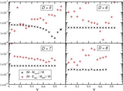
Figure 1: The normalized difference between the analytic and numerical ADM mass, $|M-M_{\rm num}|/M$ as obtained from the initial data of the Appendix for $D=5$, $6$, $7$ and $8$ and the different initial velocities is shown as black $\times$ symbols. The red $+$ symbols likewise denote deviations in the expected energy balance between the total ADM mass $M$, the horizon mass $M_{\rm AH}$ of the merger remnant BH and the radiated GW energy, i.e. $|M-E_{\rm rad}-M_{\rm AH}|/M$.

The excellent agreement (to within $10^{-4}$ or better) demonstrates consistency of the initial data with the mass energy of a boosted BH binary.

The second test addresses the energy balance throughout the entire time evolution. Assuming that the spacetime settles down to a stationary vacuum BH at late times, the ADM mass $M$ has to be equal to the sum of the postmerger remnant BH mass $M_{\rm AH}$ and the energy $E_{\rm rad}$ lost in gravitational radiation. The fractional deviation $(M-E_{\rm rad}-M_{\rm AH})/M$ from energy conservation is shown as the red $+$ symbols in Fig. 1 and demonstrates that energy is conserved in our simulations below the percent level. The accuracy of this test is limited by the discretization error of the horizon mass determined in Cook et al. (2018) to be about $0.5\,\%$ for the resolution employed here.

For the third consistency test, we have checked the convergence of the Hamiltonian constraint [see e.g. Eq. (54) in Cardoso et al. (2015)] for the specific configuration $D=8$, $v=0.6$. This choice has been motivated by the fact that we generally found it most difficult to achieve stable and accurate simulations for the case of

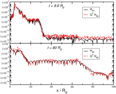
Figure 2: The Hamiltonian constraint along the collision axis for a binary with $v=0.6$ in $D=8$ dimensions. Note that only the range $x\geq 0$ is shown, as the second BH and the range $x<0$ are incorporated through reflection symmetry across the origin. The times $t=9.6\,R_{S}$ and $t=80\,R_{S}$ correspond to the infall and postmerger stages of the collision. The high-resolution results (red dashed curves) have been amplified by a factor $Q^{3}$, $Q=96/64$, to approximately match the low-resolution results, indicating convergence at about third order. The loss of convergence at $\sim 10^{-13}$ is due to roundoff error.

moderate to high velocities in $D=8$ dimensions; this is likely due to the increasingly steep gradients in the metric variables as the number of dimensions increases. In order to monitor the behavior of the constraints, we have additionally evolved this configuration with a grid resolution $h=R_{S}/64$. Figure 2 displays the violations of the Hamiltonian constraint along the collision axis at times $t=9.6\,R_{S}$ (the infall phase before merger) and $t=80\,R_{S}$ (in the postmerger ringdown phase). The high-resolution results have been amplified by a factor $Q^{3}$ with $Q=96/64$ and the resulting agreement of the curves thus obtained indicates convergence at about third order, which is in agreement with the use of fourth- and second-order ingredients in the discretization Sperhake (2007). The loss of convergence at a level of about $10^{-13}$ is due to the roundoff error of the double precision variables employed in the code. We observe the same behavior for the momentum constraint, which results in a figure very similar to Fig. 2, also showing convergence at $\approx$ third order.

In order to estimate the discretization error of our results, we have also studied the convergence of the energy $E_{\rm rad}$ radiated from this configuration in GWs. We have complemented the above simulations with a third run at resolution $h=R_{S}/48$; unlike the constraints, we do not know the continuum limit of $E_{\rm rad}$ and, hence, need this extra run. The GW energy $E_{\rm rad}$ is shown in Fig. 3.

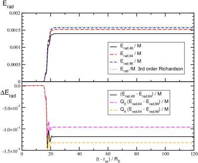
Figure 3: The energy released in gravitational radiation in the collision of a BH binary starting with $v=0.6$ in $D=8$ dimensions. (Upper panel) The results obtained for the different resolutions and the prediction obtained from third-order Richardson extrapolation. (Lower panel) The differences between the individual simulations. The high versus medium resolution differences have been amplified by factors $Q_{3}=1.947$ and $Q_{4}=2.692$ expected for third- and fourth-order convergence. The results indicate convergence in between and we estimate the uncertainty using the more conservative third-order extrapolation to the continuum limit.

The differences in $E_{\rm rad}$ indicate convergence between third and fourth order, and we estimate the uncertainty due to discretization using the more conservative third-order Richardson extrapolation. This yields a numerical uncertainty of $1.5\,\%$ for the high resolution ($h=R_{S}/96$). Note that the results of Fig. 3 contain the spurious gravitational radiation of the initial data, but this content is so small that it is not perceptible in the plots, about $10^{-7}\,M$ for this configuration. Even though its contribution can be larger, especially in $D=5$, we have found the spurious GW content to be orders of magnitude below the discretization error in all configurations. This is in marked contrast to the major role of the junk radiation in the error budget of our evolutions of conformally flat data (see e.g. Sperhake et al. (2008a)) and represents a major benefit of the superposed BH initial data.

We have analyzed two further sources of numerical uncertainties. First, the extraction of the gravitational radiation at finite radius incurs an error which we estimate through extrapolation to infinity using a series expansion in $1/r$; cf. Sec. 2 in Sperhake et al. (2011). We find this error to be about $1\,\%$ for $D=5$ and significantly lower for $D>5$. We attribute the small magnitude of this error once more to the rapid falloff of the metric fields in higher dimensions, which implies an approximately flat background metric at smaller radii than in four spacetime dimensions. Finally, we have varied the initial position of the BHs and find that the value $x_{0}=10\,R_{S}$ is sufficiently large that a further increase of $x_{0}$ leads to no significant changes in the results. In summary, we estimate the relative numerical uncertainty of our results as about $2.5\,\%$.

III.2 Numerical results and comparison with analytic calculations

The first main result of our work is displayed in Fig. 4 which shows the energy radiated in GWs from a binary with initial boost velocity $v$ in $D$ spacetime dimensions. The data have been complemented with those obtained in Ref. Sperhake et al. (2008a) for collisions in $D=4$ dimensions.

For all values $D$, two regimes are distinct in the figure. At velocities $v\lesssim 0.4$, the radiated energy shows mild variation around the rest-mass limit $E_{\rm rad}(v=0)$ whereas for $v\gtrsim 0.4$ the energy grows approximately exponentially with $v$; note the logarithmic scale on the vertical axis. Contrary to what might be expected intuitively, the lowest radiation efficiency for a given $D$ is not always realized in the rest-mass limit. For $D\geq 6$, the function

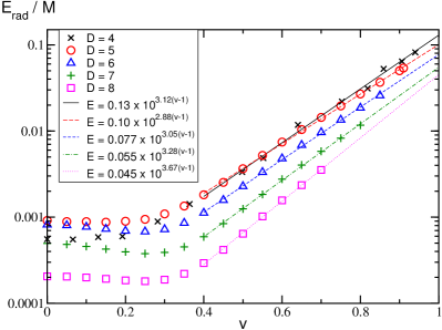
Figure 4: The energy $E_{\rm rad}$ radiated in gravitational waves from the head-on collision of two equal-mass nonspinning BHs with initial velocity $v$ in $D$ spacetime dimensions. The fits have been computed from data with $v\geq 0.4$ assuming a functional relation $\log E_{\rm rad}=a_{0}+a_{1}v$. The results have been rewritten to facilitate easy reading of the limit $E_{\rm rad}(v\rightarrow 1)$.

$E_{\rm rad}(v)$ exhibits a minimum at finite $v\approx 0.25$. This behavior has in fact already been noticed in point-particle calculations by Berti et al. Berti et al. (2011). In their Fig. 1, the energy radiated in collisions starting from rest exceeds that for mild boost velocities for $D\geq 6$; note that, contrary to our Fig. 4, their horizontal axis denotes the number of dimensions while different symbols mark the velocity. For $D=11$, their rest-mass case produces even more radiation than the ultrarelativistic limit. Our dataset does not allow a clear verification of whether this unexpected phenomenon persists in the comparable mass limit, but applying fits to our numerical data confirms that the radiative efficiency in the ultrarelativistic limit decreases for larger $D$.

For our fits, we have considered only data at $v\geq 0.4$, where we observe an approximately linear growth of $\log E_{\rm rad}$ with $v$. We therefore apply for each value of $D$ a regression of the form

$$\log E_{\rm rad}=a_{0}+a_{1}v\,.$$ (2)

It is straightforward to translate the resulting coefficients into the following notation, where the coefficient in front represents the limit $E_{\rm rad}(v\rightarrow 1)$,

$$E_{\rm rad}=(0.129\pm 0.03)\times 10^{(3.12\pm 0.05)(v-1)}~{} \text{ in }D=4$$

$$E_{\rm rad}=(0.101\pm 0.010)\times 10^{(2.88\pm 0.03)(v-1)}~{} \text{ in }D=5$$

$$E_{\rm rad}=(0.077\pm 0.008)\times 10^{(3.05\pm 0.03)(v-1)}~{} \text{ in }D=6$$

$$E_{\rm rad}=(0.055\pm 0.005)\times 10^{(3.28\pm 0.03)(v-1)}~{} \text{ in }D=7$$

$$E_{\rm rad}=(0.045\pm 0.008)\times 10^{(2.88\pm 0.05)(v-1)}~{} \text{ in }D=8\,.$$

The minor deviation of the result for $D=4$ in this list from the ultrarelativistic limit reported in Sperhake et al. (2008a) is due to the different functional relations employed in the fits.

It has been noted in Ref. Cook et al. (2017) that the overall reduction of the radiated energy with increasing $D$ bears a qualitative resemblance to the decreasing surface area of the $D$ dimensional unit sphere, $\mathcal{A}_{D-2}=2\pi^{(D-1)/2}\,/\,\Gamma[(D-1)/2]$. The $D$ dependence of the radiation efficiency, however, will also be affected by the increasingly steep strong-field gradients in larger $D$. These would be expected to result in more violent interaction, but also imply that this interaction occurs increasingly close to merger such that more of the strong-field dynamics are captured inside the common apparent horizon and cannot radiate to infinity. The net impact of these competing effects is not obvious, but our numerical results demonstrate dominance of those effects reducing $E_{\rm rad}$.

We next investigate whether our data confirm the intriguing observation by Okawa et al. Okawa et al. (2011) that

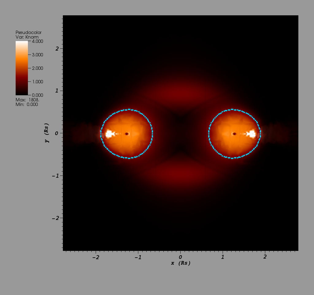
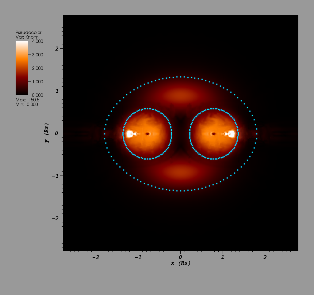
Figure 5: The normalized Kretschmann scalar $\mathcal{K}/\mathcal{K}_{p}$ at times $t=12.8\,R_{S}$ (left) and $t=13.3\,R_{S}$ (right panel) in the collision of a binary with $v=0.85$ in $D=6$ dimensions. The light-blue lines show the apparent horizon. At $t=12.8\,R_{S}$ two regions where $\mathcal{K}>1$ form, one above and one below the collision axis, indicating that super-Planckian curvature may become visible outside the BH horizon. At $t=13.3$ a common horizon has formed and engulfed this region.

high-energy BH collisions in higher dimensions may form regions of super-Planckian curvature that are not hidden inside an event horizon. For this analysis, Okawa et al. compute the Kretschmann scalar $\mathcal{K}^{2}\mathrel{\vbox{\hbox{\scriptsize.}\hbox{\scriptsize.}}}=R^{{\scriptscriptstyle{A}}{\scriptscriptstyle{B}}{\scriptscriptstyle{C}}{\scriptscriptstyle{D}}}R_{{\scriptscriptstyle{A}}{\scriptscriptstyle{B}}{\scriptscriptstyle{C}}{\scriptscriptstyle{D}}}$ (where $A,\,B,\,\ldots=0,\,\ldots,\,D-1$) and normalize the result with the corresponding value obtained on the horizon of a BH with a mass equal to the Planck mass. Their Fig. 2 displays the Kretschmann scalar thus normalized, and identifies a region of super-Planckian curvature around the origin and outside the BHs’ apparent horizons.

We have explored this phenomenon for our head-on collision with $v=0.85$ in $D=6$ dimensions. Some care is required in the comparison, however, because we use the convention of Emparan and Reall (2008) and write the Einstein equations as $G_{{\scriptscriptstyle{A}}{\scriptscriptstyle{B}}}=8\pi GT_{{\scriptscriptstyle{A}}{\scriptscriptstyle{B}}}$ for all values of $D$, which mildly differs from the convention of Okawa et al. (2011). For our choice, the mass of a Tangherlini BH with mass parameter $\mu$ is given by Eq. (1). We regard a BH as in the Planckian regime if its Compton wavelength $1/M_{p}$ (recall that we set $\hbar=c=1$) is equal to its horizon radius, i.e.

$$\frac{1}{M_{p}^{D-3}}\overset{!}{=}r_{S}^{D-3}=\mu=\frac{16\pi GM_{p}}{(D-2)\Omega_{D-2}}$$ (4)

$$\Rightarrow M_{p}^{D-2}=\frac{(D-2)\Omega_{D-2}}{16\pi G}\,.$$

For $D=6$, we thus obtain for the Planck mass $M_{p}^{4}=2\pi/(3G)$. The Kretschmann scalar on the horizon of a Tangherlini BH in $D=6$ dimensions is

$$\mathcal{K}^{2}=\frac{240\mu^{2}}{r^{10}}\,.$$ (5)

In this expression we first substitute for $\mu$ in terms of the BH mass through Eq. (1), and then insert for $M$ the Planck mass $M_{p}$ obtained from Eq. (4). The result gives the Kretschmann scalar on the horizon of a BH with mass $M_{p}$ as

$$\mathcal{K}_{p}^{2}=\frac{180\pi}{G}\,.$$ (6)

Following Ref. Okawa et al. (2011) we have computed the normalized $\mathcal{K}/\mathcal{K}_{p}$ and show in Fig. 5 the result in the $xy$ plane; we recall that this plane is orthogonal to the $z$ direction, i.e. the quasiradial direction associated with our rotational isometry Cook et al. (2016). The apparent horizon is displayed in the figure with light blue, dashed curves and contains the regions of highest curvature. Shortly before we first find a common apparent horizon, however, two regions of significant curvature $\mathcal{K}>\mathcal{K}_{p}$ have formed above and below the collision axis (left panel in Fig. 5). This region is eventually enclosed inside the common apparent horizon that we first observe at $t=13.3~{}R_{S}$ in the right panel. Our evidence for regions of super-Planckian curvature is less strong than that presented in Okawa et al. (2011) because our failure to find an apparent horizon at $t=12.8~{}R_{S}$ in the left panel of Fig. 5 does not prove that an apparent horizon does not exist. The simulation presented in Okawa et al. (2011), in contrast, represents a scattering configuration, which demonstrates more clearly that a common horizon is not present at the time of super-Planckian curvature. Nonetheless, our results support their observations, and indicate that super-Planckian curvature outside a cloaking horizon may also form in head-on collisions of BHs and in $D>5$. Theoretically, there is no reason why super-Planckian curvature outside a BH horizon cannot occur in $D=4$, but we are not aware of a case where this has been observed.

IV Conclusions

In this study we have modeled head-on collisions of nonspinning, equal-mass BH binaries with boost velocities up to $v_{\rm max}=0.91~{}(0.85,~{}0.8,~{}0.7)$ in $D=5~{}(6,~{}7,~{}8)$ spacetime dimensions. By using initial data constructed from superposed Lorentz boosted Tangherlini BH solutions in isotropic coordinates, we have managed to significantly reduce the amount of spurious gravitational radiation as compared with conformally flat initial data of Bowen-York type. We have verified the suitability of these initial data by confirming conservation of the total mass energy and convergence of the Einstein constraints (Figs. 1 and 2). We estimate the relative numerical error of our results to be about $2.5\,\%$ (Fig. 3, Sec. III.1). By also including previous results obtained for boosted head-on collisions in $D=4$ dimensions Sperhake et al. (2008a), our main findings are summarized as follows.

• Independent of the number of spacetime dimensions, we identify two distinct regimes: For initial boosts $v\lesssim 0.4$, the radiated GW energy only mildly deviates from the limit of collisions starting from rest. For $v\gtrsim 0.4$, the radiated energy grows approximately exponentially with the velocity parameter $v$ (Fig. 4).

• In agreement with point-particle calculations Berti et al. (2011), we find that for $D\geq 6$, the radiated energy as a function of initial velocity reaches a local minimum for mild but finite boosts $v\approx 0.25$ (Fig. 4).

• By extrapolating the numerical results to the ultrarelativistic limit $v\rightarrow 1$, we find that head-on collisions of equal-mass, nonspinning BHs radiate $12.9\,\%$, $10.1\,\%$, $7.7\,\%$, $5.5\,\%$, $4.5\,\%$ of the total energy in the center-of-mass frame, respectively, in $D=4,~{}5,~{}6,~{}7,~{}8$ dimensions; cf. Eq. (LABEL:eq:Erad).

• By computing the Kretschmann curvature scalar for head-on collisions in $D=6$ dimensions with initial boost $v=0.85$, we identify regions with super-Planckian curvature outside the apparent horizon, supporting previous numerical results Okawa et al. (2011) which show “visible” regions of super-Planckian curvature in grazing BH collisions in $D=5$.

Our results for the radiated energy demonstrate that high-energy collisions of BHs can radiate considerable amounts of energy even in higher dimensions. On the other hand, the values we find are significantly lower than the remarkable $E_{\rm rad}/M=\frac{1}{2}-\frac{1}{D}$ formula derived from first-order perturbative calculations of shock-wave collisions Coelho et al. (2012, 2014). In $D=4$, the inclusion of second-order terms in the perturbative calculations has lowered the radiation estimate from $E_{\rm rad}^{(1)}=25\,\%$ to $E_{\rm rad}^{(2)}=16.4\,\%$ D’Eath (1978); D’Eath and Payne (1992c). First steps have been taken to extend the $D>4$ case to second order Coelho et al. (2014). It will be interesting to see if estimates of the total radiated energy will lead to a similar reduction and, thus, close the gap between numerical relativity and shock-wave calculations. Our numerical results suggest that relatively simple BH production scenarios based on cross sections derived from the (higher-dimensional) Schwarzschild radius Sirunyan et al. (2018); Giddings and Thomas (2002) would require only mild modifications by a factor close to unity in order to account for energy loss through gravitational radiation.

Results in $D=4$ have shown that grazing collisions may emit gravitational waves more efficiently than the head-on limit; to compute whether this also holds in higher dimensions is one of the main questions to be addressed in future work. A further extension of our work may consider boosted collisions of BHs in higher-dimensional Lovelock gravity following the BH solutions and formalism of Refs. Dadhich (2011); Dadhich et al. (2013); Dadhich (2016). Such a program, however, might require more investigation to ensure availability of a well-posed initial-value formulation Papallo and Reall (2017); Papallo (2018-03-29).

Appendix A INITIAL DATA FOR BOOSTED BLACK-HOLE BINARIES

In this section we need a wider set of indices to distinguish between spacetime and spatial, as well as between on- and off-domain spatial indices. More specifically, we use capital early (middle) latin indices to cover all spacetime (spatial) dimensions. Lowercase middle latin indices cover the three spatial directions inside our computational domain, and early latin indices the extra dimensions outside the computational domain. Greek indices include time and the on-domain directions. For $D$ spacetime dimensions, our indices therefore have the following ranges:

$$A,~{}B,\ldots=0,\,\ldots,\,D-1\,;~{}~{}~{} I,~{}J,\ldots=1,\,\ldots,\,D-1\,;$$ (7)

$$i,~{}j,\ldots=1,\,2,\,3\,;~{}~{}~{} a,~{}b,\ldots=4,\,\ldots,\,D-1\,.$$

$$\alpha,~{}\beta,\ldots=0,\,1,\,2,\,3\,.$$

Our starting point is the Tangherlini metric that describes a $D$-dimensional, spherically symmetric BH with mass parameter $\mu$ in radial gauge and polar slicing,

$$ds^{2}=-\left(1-\frac{\mu}{R^{D-3}}\right)dt^{2}+\left(1-\frac{\mu}{R^{D-3}}\right)^{-1}dR^{2}+R^{2}d\omega^{2}_{D-2}\,,$$ (8)

where $d\omega^{2}_{D-2}$ denotes the line element of the $D-2$ sphere. The metric in isotropic coordinates is obtained by transforming the radial coordinate according to

$$R=r\left(1+\frac{\mu}{4r^{D-3}}\right)^{\frac{2}{D-3}}\,,$$ (9)

which leads to the metric

$$ds^{2}=-\Omega^{2}\Psi^{-2}dt^{2}+\Psi^{\frac{4}{D-3}}(dr^{2}+r^{2}d\omega_{D-2}^{2})$$

$$\hphantom{ds^{2}}=-\Omega^{2}\Psi^{-2}dt^{2}+\Psi^{\frac{4}{D-3}}[(dx^{1})^{2}+\ldots+(dx^{D-1})^{2}]\,,$$

$$\Omega=1-\frac{\mu}{4r^{D-3}}\,,~{}~{}~{}~{}~{}~{}~{}~{}~{}~{}\Psi=1+\frac{\mu}{4r^{D-3}}\,.$$ (10)

where $x^{1},\,\ldots,\,x^{D-1}$ are standard Cartesian coordinates with $r^{2}=(x^{1})^{2}+\ldots+(x^{D-1})^{2}$.

In the ADM formalism Arnowitt et al. (1962); York (1979), the spacetime metric is written in terms of the lapse function $\alpha$, the shift vector $\beta^{I}$ and the spatial metric $\gamma_{IJ}$ according to

$$g_{AB}=\left(\begin{array}[]{c|c}-\alpha^{2}+\beta_{M}\beta^{M}&\beta_{J}\\[3.0pt] \hline\cr\\[-7.0pt] \beta_{I}&\gamma_{IJ}\end{array}\right)=\left(\begin{array}[]{c|c|c}-\alpha^{2}+\beta_{m}\beta^{m}&\beta_{j}&0\\[5.0pt] \hline\cr\\[-7.0pt] \beta_{i}&\gamma_{ij}&0\\[5.0pt] \hline\cr\\[-7.0pt] 0&0&\gamma_{ww}\delta_{ab}\end{array}\right)\,,$$ (11)

where the first expression is general, and the second accounts for the simplifications due to $SO(D-3)$ isometry. For the inverse metric we likewise have

$$g^{{\scriptscriptstyle{A}}{\scriptscriptstyle{B}}}=\left(\begin{array}[]{c|c}-\alpha^{-2}&\alpha^{-2}\beta^{{\scriptscriptstyle{J}}}\\[3.0pt] \hline\cr\\[-7.0pt] \alpha^{-2}\beta^{{\scriptscriptstyle{I}}}&\gamma^{{\scriptscriptstyle{I}}{\scriptscriptstyle{J}}}-\alpha^{-2}\beta^{{\scriptscriptstyle{I}}}\beta{{}^{\scriptscriptstyle{J}}}\end{array}\right)=\left(\begin{array}[]{c|c|c}\alpha^{-2}&\alpha^{-2}\beta^{j}&0\\[5.0pt] \hline\cr\\[-7.0pt] \alpha^{-2}\beta^{i}&\gamma^{ij}-\alpha^{-2}\beta^{i}\beta^{j}&0\\[5.0pt] \hline\cr\\[-7.0pt] 0&0&\gamma^{ww}\delta^{ab}\end{array}\right)\,.$$ (12)

Here $w$ is not an index: $\gamma_{ww}$ and $\gamma^{ww}=1\,/\,\gamma_{ww}$ merely denote the single extra variable for the metric and inverse metric needed to describe the geometry in the extra dimensions. We also note that $\gamma^{ij}$ is the inverse of $\gamma_{ij}$, and $\gamma^{{\scriptscriptstyle{I}}{\scriptscriptstyle{J}}}$ the inverse of $\gamma_{{\scriptscriptstyle{I}}{\scriptscriptstyle{J}}}$.

By equating (11) and (12) with the Cartesian metric of Eq. (10), we obtain the components for the lapse, shift and spatial metric

$$\alpha=\Omega\Psi^{-1}\,,~{}~{}~{}~{}~{}~{}~{}~{} \beta^{i}=\beta^{a}=0\,,$$ (13)

$$\gamma_{ij}=\Psi^{\frac{4}{D-3}}\,\delta_{ij}\,,~{}~{}~{}~{}~{}~{}~{}~{} \gamma_{ia}=0\,,$$

$$\gamma_{ab}=\gamma_{ww}\,\delta_{ab}\,,~{}~{}~{}~{}~{}~{}~{}~{} \gamma_{ww}=\Psi^{\frac{4}{D-3}}\,.$$

The extrinsic curvature has a more complicated relation to the metric and also involves derivatives. We use the sign convention where

$$K_{{\scriptscriptstyle{I}}{\scriptscriptstyle{J}}}=-\frac{1}{2\alpha}\left(\partial_{0}\gamma_{{\scriptscriptstyle{I}}{\scriptscriptstyle{J}}}-\beta^{{\scriptscriptstyle{M}}}\partial_{{\scriptscriptstyle{M}}}\gamma_{{\scriptscriptstyle{I}}{\scriptscriptstyle{J}}}-\gamma_{{\scriptscriptstyle{M}}{\scriptscriptstyle{J}}}\partial_{{\scriptscriptstyle{I}}}\beta^{{\scriptscriptstyle{M}}}-\gamma_{{\scriptscriptstyle{I}}{\scriptscriptstyle{M}}}\partial_{{\scriptscriptstyle{J}}}\beta^{{\scriptscriptstyle{M}}}\right)\,.$$ (14)

Applied to the Tangherlini metric (10), however, one directly finds that $K_{{\scriptscriptstyle{I}}{\scriptscriptstyle{J}}}=0$, because the metric is time independent and has zero shift vector.

The next step in our initial data construction consists of applying a Lorentz boost to the Tangherlini metric in Cartesian coordinates. For this purpose we consider an observer $\mathcal{O}$ in the rest frame of the BH, and a second observer $\tilde{\mathcal{O}}$ who moves with velocity $-v^{{\scriptscriptstyle{I}}}$ relative to $\mathcal{O}$. The transformation between the two frames is given by

$$x^{\tilde{{\scriptscriptstyle{A}}}}=\Lambda^{\tilde{{\scriptscriptstyle{A}}}}{}_{{\scriptscriptstyle{E}}}x^{{\scriptscriptstyle{E}}}+x_{0}^{\tilde{{\scriptscriptstyle{A}}}}~{}~{}~{}~{}~{}\Leftrightarrow~{}~{}~{}~{}~{}x^{{\scriptscriptstyle{E}}}=\Lambda^{{\scriptscriptstyle{E}}}{}_{\tilde{{\scriptscriptstyle{A}}}}(x^{\tilde{{\scriptscriptstyle{A}}}}-x_{0}^{\tilde{{\scriptscriptstyle{A}}}})\,,$$ (15)

where

$$\Lambda^{\tilde{{\scriptscriptstyle{A}}}}{}_{{\scriptscriptstyle{E}}}=\left(\begin{array}[]{c|c}\Lambda^{\tilde{\alpha}}{}_{\epsilon}&0\\[3.0pt] \hline\cr\\[-7.0pt] 0&\delta^{\tilde{a}}{}_{e}\end{array}\right)=\left(\begin{array}[]{c|c|c}\gamma&\gamma v_{j}&0\\[3.0pt] \hline\cr\\[-7.0pt] \gamma v^{i}&\delta^{i}{}_{j}+(\gamma-1)\frac{v^{i}v_{j}}{|\vec{v}|^{2}}&0\\[5.0pt] \hline\cr\\[-7.0pt] 0&0&\delta^{\tilde{a}}{}_{e}\end{array}\right)\,,$$ (16)

and its inverse $\Lambda^{{\scriptscriptstyle{E}}}{}_{\tilde{{\scriptscriptstyle{A}}}}$ is obtained from the same expression by simply inverting the sign of the velocity $v^{i}$. Note that boosts in the extra dimensions are excluded here in order to preserve the $SO(D-3)$ isometry. Without loss of generality, we will from now on set the constant offset $x_{0}^{\tilde{A}}$ to zero, which merely implies synchronization of the two observers’ clocks when they meet.

The metric components and their derivatives in the two frames $\mathcal{O}$ and $\tilde{\mathcal{O}}$ are related by

$$g_{\tilde{{\scriptscriptstyle{A}}}\tilde{{\scriptscriptstyle{B}}}} = \Lambda^{{\scriptscriptstyle{E}}}{}_{\tilde{{\scriptscriptstyle{A}}}}\Lambda^{{\scriptscriptstyle{F}}}{}_{\tilde{{\scriptscriptstyle{B}}}}\,g_{{\scriptscriptstyle{E}}{\scriptscriptstyle{F}}}\,,$$ (17)

$$\partial_{\tilde{{\scriptscriptstyle{C}}}}g_{\tilde{{\scriptscriptstyle{A}}}\tilde{{\scriptscriptstyle{B}}}} = \Lambda^{{\scriptscriptstyle{G}}}{}_{\tilde{{\scriptscriptstyle{C}}}}\Lambda^{{\scriptscriptstyle{E}}}{}_{\tilde{{\scriptscriptstyle{A}}}}\Lambda^{{\scriptscriptstyle{F}}}{}_{\tilde{{\scriptscriptstyle{B}}}}\,\partial_{{\scriptscriptstyle{G}}}g_{{\scriptscriptstyle{E}}{\scriptscriptstyle{F}}}\,.$$ (18)

For the eventual calculation, it is convenient to consider separately in these relations the spacetime components inside our computational domain and those corresponding to the off-domain directions $x^{a}$. This leads to the following transformation rules for the metric, its inverse and its partial derivatives,

$$g_{\tilde{\alpha}\tilde{\beta}}=\Lambda^{\mu}{}_{\tilde{\alpha}}\Lambda^{\nu}{}_{\tilde{\beta}}g_{\mu\nu}\,,~{}~{} g_{\tilde{a}\tilde{b}}=\delta_{\tilde{a}\tilde{b}}\,g_{ww}\,,$$

$$g^{\tilde{\alpha}\tilde{\beta}}=\Lambda^{\tilde{\alpha}}{}_{\mu}\Lambda^{\tilde{\beta}}{}_{\nu}g^{\mu\nu}\,,~{}~{} g^{\tilde{a}\tilde{b}}=\delta^{\tilde{a}\tilde{b}}g^{ww}\,,$$

$$\partial_{\tilde{\gamma}}g_{\tilde{\alpha}\tilde{\beta}}=\Lambda^{\lambda}{}_{\tilde{\gamma}}\Lambda^{\mu}{}_{\tilde{\alpha}}\Lambda^{\nu}{}_{\tilde{\beta}}\partial_{\lambda}g_{\mu\nu}\,,~{}~{} \partial_{\tilde{\gamma}}g_{\tilde{a}\tilde{b}}=\Lambda^{\lambda}{}_{\tilde{\gamma}}\delta_{\tilde{a}\tilde{b}}\partial_{\lambda}g_{ww}\,,$$

with all other components and derivatives being manifestly zero. The ADM variables in the boosted frame $\tilde{\mathcal{O}}$ can then be read off from these expressions through the relations (11), (12) and (14), which hold in exactly the same form in the new coordinates $x^{\tilde{\alpha}}$. This gives us

$$\tilde{\alpha}=\big{(}-g^{\tilde{0}\tilde{0}}\big{)}^{-1/2}\,,~{}~{}~{}~{}~{}\beta_{\tilde{i}}=g_{\tilde{0}\tilde{i}}\,,~{}~{}~{}~{}~{}\gamma_{\tilde{i}\tilde{j}}=g_{\tilde{i}\tilde{j}}\,,$$

$$\gamma_{\tilde{a}\tilde{b}}=\gamma_{\tilde{w}\tilde{w}}\,\delta_{\tilde{a}\tilde{b}}\,,~{}~{}~{}~{}~{}\gamma_{\tilde{w}\tilde{w}}=g_{\tilde{w}\tilde{w}}=g_{ww}\,,$$

$$K_{\tilde{i}\tilde{j}}=\frac{-1}{2\tilde{\alpha}}\left(\partial_{\tilde{0}}\gamma_{\tilde{i}\tilde{j}}-\beta^{\tilde{m}}\partial_{\tilde{m}}\gamma_{\tilde{i}\tilde{j}}-\gamma_{\tilde{m}\tilde{j}}\partial_{\tilde{i}}\beta^{\tilde{m}}-\gamma_{\tilde{i}\tilde{m}}\partial_{\tilde{j}}\beta^{\tilde{m}}\right)\,,$$

$$K_{\tilde{a}\tilde{b}}=K_{\tilde{w}\tilde{w}}\,\delta_{\tilde{a}\tilde{b}}\,.$$

$$K_{\tilde{w}\tilde{w}}=\frac{-1}{2\tilde{\alpha}}\left(\partial_{\tilde{0}}\gamma_{\tilde{w}\tilde{w}}-\beta^{\tilde{m}}\partial_{\tilde{m}}\gamma_{\tilde{w}\tilde{w}}-2\gamma_{\tilde{w}\tilde{w}}\frac{\beta^{\tilde{z}}}{\tilde{z}}\right)\,.$$ (20)

Note that we have put a tilde on the index free lapse function $\tilde{\alpha}$ to distinguish it from the lapse $\alpha$ in the rest frame $\mathcal{O}$, and that we have used in the last line the relation Cook et al. (2016)

$$\lim_{z\rightarrow 0}\partial_{a}\beta^{c}=\frac{\beta^{z}}{z}\delta_{a}{}^{c}\,.$$ (21)

This transformation allows us to compute the initial data for a single boosted BH. For binary data, we compute such a solution for two BHs $\mathcal{A}$ and $\mathcal{B}$ with opposite boost velocities $v_{\mathcal{B}}^{i}=-v_{\mathcal{A}}^{i}$ and initially located at positions $x_{\mathcal{A}}^{i}=-x_{\mathcal{B}}^{i}$, which gives us the center-of-mass frame for equal-mass BHs. Following Sperhake et al. (2005), we construct superposed binary data from the two individual solutions according to

$$\gamma_{\tilde{i}\tilde{j}} = \gamma_{\tilde{i}\tilde{j}}^{\mathcal{A}}+\gamma_{\tilde{i}\tilde{j}}^{\mathcal{B}}-\delta_{\tilde{i}\tilde{j}}\,,$$

$$\hat{K}^{\tilde{i}}{}_{\tilde{j}} = K^{\tilde{i}}{}_{\tilde{j}}{}^{\mathcal{A}}+K^{\tilde{i}}{}_{\tilde{j}}{}^{\mathcal{B}}\,,$$

$$K_{\tilde{i}\tilde{j}} = \frac{1}{2}\left(\gamma_{\tilde{i}\tilde{m}}\hat{K}^{\tilde{m}}{}_{\tilde{j}}+\gamma_{\tilde{j}\tilde{m}}\hat{K}^{\tilde{m}}{}_{\tilde{i}}\right)\,.$$ (22)

Instead of superposing the lapse and shift vector in an analogous way, we initialize the lapse in terms of the conformal factor of the BSSNOK formulation, $\tilde{\alpha}=\sqrt{\tilde{\chi}}\,,~{}~{}\tilde{\chi}=(\det\gamma_{\tilde{i}\tilde{j}})^{-1/(D-1)}$, and set the initial shift to zero, $\beta^{\tilde{i}}=0$.

References

- Arkani-Hamed et al. (1998) N. Arkani-Hamed, S. Dimopoulos, and G. R. Dvali, Phys. Lett. B 429, 263 (1998), hep-ph/9803315.
- Antoniadis (1990) I. Antoniadis, Phys. Lett. B 246, 377 (1990).
- Antoniadis et al. (1998) I. Antoniadis, N. Arkani-Hamed, S. Dimopoulos, and G. R. Dvali, Phys. Lett. B 436, 257 (1998), hep-ph/9804398.
- Banks and Fischler (1999) T. Banks and W. Fischler (1999), hep-th/9906038.
- Giddings and Thomas (2002) S. B. Giddings and S. Thomas, Phys. Rev. D 65, 056010 (2002), hep-ph/0106219.
- Dimopoulos and Landsberg (2001) S. Dimopoulos and G. Landsberg, Phys. Rev. Lett. 87, 161602 (2001), hep-th/0106295.
- Hawking (1971) S. W. Hawking, Phys. Rev. Lett. 26, 1344 (1971).
- Penrose (1974) R. Penrose (1974), presented at the Cambridge University Seminar, Cambridge, England (unpublished).
- D’Eath and Payne (1992a) P. D. D’Eath and P. N. Payne, Phys. Rev. D 46, 658 (1992a).
- Eardley and Giddings (2002) D. M. Eardley and S. B. Giddings, Phys. Rev. D 66, 044011 (2002), gr-qc/0201034.
- Arnowitt et al. (1962) R. Arnowitt, S. Deser, and C. W. Misner, in Gravitation an introduction to current research, edited by L. Witten (John Wiley, New York, 1962), pp. 227–265, gr-qc/0405109.
- D’Eath (1978) P. D. D’Eath, Phys. Rev. D 18, 990 (1978).
- D’Eath and Payne (1992b) P. D. D’Eath and P. N. Payne, Phys. Rev. D 46, 675 (1992b).
- D’Eath and Payne (1992c) P. D. D’Eath and P. N. Payne, Phys. Rev. D 46, 694 (1992c).
- Herdeiro et al. (2011) C. Herdeiro, M. O. P. Sampaio, and C. Rebelo, JHEP 1107, 121 (2011), arXiv:1105.2298 [hep-th].
- Coelho et al. (2013) F. S. Coelho, C. Herdeiro, C. Rebelo, and M. Sampaio, Phys. Rev. D 87, 084034 (2013), arXiv:1206.5839 [hep-th].
- Coelho et al. (2012) F. S. Coelho, C. Herdeiro, and M. O. P. Sampaio, Phys. Rev. Lett. 108, 181102 (2012), arXiv:1203.5355 [hep-th].
- Coelho et al. (2014) F. S. Coelho, C. Herdeiro, and M. O. P. Sampaio, JHEP 12, 119 (2014), arXiv:1410.0964 [hep-th].
- Anninos et al. (1993) P. Anninos, D. Hobill, E. Seidel, L. Smarr, and W.-M. Suen, Phys. Rev. Lett. 71, 2851 (1993), gr-qc/9309016.
- Sperhake et al. (2008a) U. Sperhake, V. Cardoso, F. Pretorius, E. Berti, and J. A. González, Phys. Rev. Lett. 101, 161101 (2008a), arXiv:0806.1738 [gr-qc].
- Sperhake et al. (2016) U. Sperhake, E. Berti, V. Cardoso, and F. Pretorius, Phys. Rev. D 93, 044012 (2016), arXiv:1511.08209 [gr-qc].
- Healy et al. (2016) J. Healy, I. Ruchlin, C. O. Lousto, and Y. Zlochower, Phys. Rev. D 94, 104020 (2016), eprint arXiv:1506.06153 [gr-qc].
- Shibata et al. (2008) M. Shibata, H. Okawa, and T. Yamamoto, Phys. Rev. D 78, 101501(R) (2008), arXiv:0810.4735 [gr-qc].
- Sperhake et al. (2009) U. Sperhake, V. Cardoso, F. Pretorius, E. Berti, T. Hinderer, and N. Yunes, Phys. Rev. Lett. 103, 131102 (2009), arXiv:0907.1252 [gr-qc].
- Sperhake et al. (2013) U. Sperhake, E. Berti, V. Cardoso, and F. Pretorius, Phys. Rev. Lett. 111, 041101 (2013), arXiv:1211.6114 [gr-qc].
- Glampedakis and Kennefick (2002) K. Glampedakis and D. Kennefick, Phys. Rev. D 66, 044002 (2002), gr-qc/0203086.
- Pretorius and Khurana (2007) F. Pretorius and D. Khurana, Class. Quantum Grav. 24, S83 (2007), gr-qc/0702084.
- Choptuik and Pretorius (2010) M. W. Choptuik and F. Pretorius, Phys. Rev. Lett. 104, 111101 (2010), arXiv:0908.1780 [gr-qc].
- East and Pretorius (2013) W. E. East and F. Pretorius, Phys. Rev. Lett. 110, 101101 (2013), arXiv:1210.0443 [gr-qc].
- Rezzolla and Takami (2013) L. Rezzolla and K. Takami, Class. Quant. Grav. 30, 012001 (2013), arXiv:1209.6138 [gr-qc].
- Pretorius (2005a) F. Pretorius, Phys. Rev. Lett. 95, 121101 (2005a), gr-qc/0507014.
- Baker et al. (2006) J. G. Baker, J. Centrella, D.-I. Choi, M. Koppitz, and J. van Meter, Phys. Rev. Lett. 96, 111102 (2006), gr-qc/0511103.
- Campanelli et al. (2006) M. Campanelli, C. O. Lousto, P. Marronetti, and Y. Zlochower, Phys. Rev. Lett. 96, 111101 (2006), gr-qc/0511048.
- Cardoso et al. (2015) V. Cardoso, L. Gualtieri, C. Herdeiro, and U. Sperhake, Living Rev. Relativity 18, 1 (2015), arXiv:1409.0014 [gr-qc].
- Barack et al. (2019) L. Barack et al., Class. Quant. Grav. 36, 143001 (2019), eprint arXiv:1806.05195 [gr-qc].
- Shibata and Yoshino (2010) M. Shibata and H. Yoshino, Phys. Rev. D 81, 104035 (2010), arXiv:1004.4970 [gr-qc].
- Lehner and Pretorius (2010) L. Lehner and F. Pretorius, Phys. Rev. Lett. 105, 101102 (2010), arXiv:1006.5960 [hep-th].
- Figueras et al. (2016) P. Figueras, M. Kunesch, and S. Tunyasuvunakool, Phys. Rev. Lett. 116, 071102 (2016), arXiv:1512.04532 [hep-th].
- Figueras et al. (2017) P. Figueras, M. Kunesch, L. Lehner, and S. Tunyasuvunakool, Phys. Rev. Lett. 118, 151103 (2017), eprint arXiv:1702.01755 [hep-th].
- Bantilan et al. (2019) H. Bantilan, P. Figueras, M. Kunesch, and R. Panosso Macedo, Phys. Rev. D 100, 086014 (2019), eprint 1906.10696.
- Witek et al. (2010) H. Witek, M. Zilhão, L. Gualtieri, V. Cardoso, C. Herdeiro, A. Nerozzi, and U. Sperhake, Phys. Rev. D 82, 104014 (2010), arXiv:1006.3081 [gr-qc].
- Cook et al. (2017) W. G. Cook, U. Sperhake, E. Berti, and V. Cardoso, Phys. Rev. D 96, 124006 (2017), eprint arXiv:1709.10514 [gr-qc].
- Okawa et al. (2011) H. Okawa, K.-i. Nakao, and M. Shibata, Phys. Rev. D 83, 121501(R) (2011), arXiv:1105.3331 [gr-qc].
- Zilhão et al. (2011) M. Zilhão, M. Ansorg, V. Cardoso, L. Gualtieri, C. Herdeiro, U. Sperhake, and H. Witek, Phys. Rev. D 84, 084039 (2011), arXiv:1109.2149 [gr-qc].
- Cook et al. (2018) W. G. Cook, D. Wang, and U. Sperhake, Class. Quant. Grav. 35, 235008 (2018), eprint arXiv:1808.05834 [gr-qc].
- Sperhake (2007) U. Sperhake, Phys. Rev. D 76, 104015 (2007), gr-qc/0606079.
- Sperhake et al. (2008b) U. Sperhake, E. Berti, V. Cardoso, J. A. González, B. Brügmann, and M. Ansorg, Phys. Rev. D 78, 064069 (2008b), arXiv:0710.3823 [gr-qc].
- Nakamura et al. (1987) T. Nakamura, K. Oohara, and Y. Kojima, Prog. Theor. Phys. Suppl. 90, 1 (1987).
- Shibata and Nakamura (1995) M. Shibata and T. Nakamura, Phys. Rev. D 52, 5428 (1995).
- Baumgarte and Shapiro (1998) T. W. Baumgarte and S. L. Shapiro, Phys. Rev. D 59, 024007 (1998), gr-qc/9810065.
- Allen, G. and Goodale, T. and Massó, J. and Seidel, E. (1999) Allen, G. and Goodale, T. and Massó, J. and Seidel, E., in Proceedings of Eighth IEEE International Symposium on High Performance Distributed Computing, HPDC-8, Redondo Beach, 1999 (IEEE Press, , 1999).
- zzz (001) zzz001, Cactus Computational Toolkit homepage: http://www.cactuscode.org/.
- zzz (002) zzz002, Carpet Code homepage: http://www.carpetcode.org/.
- Schnetter et al. (2004) E. Schnetter, S. H. Hawley, and I. Hawke, Class. Quant. Grav. 21, 1465 (2004), gr-qc/0310042.
- Pretorius (2005b) F. Pretorius, Class. Quantum Grav. 22, 425 (2005b), gr-qc/0407110.
- Zilhão et al. (2010) M. Zilhão, H. Witek, U. Sperhake, V. Cardoso, L. Gualtieri, C. Herdeiro, and A. Nerozzi, Phys. Rev. D 81, 084052 (2010), arXiv:1001.2302 [gr-qc].
- Yoshino and Shibata (2011a) H. Yoshino and M. Shibata, Prog.Theor.Phys.Suppl. 189, 269 (2011a).
- Yoshino and Shibata (2011b) H. Yoshino and M. Shibata, Prog.Theor.Phys.Suppl. 190, 282 (2011b).
- Zilhão (2012) M. Zilhão, Ph.D. thesis, University of Porto (2012), arXiv:1301.1509 [gr-qc].
- Alcubierre et al. (2001) M. Alcubierre, S. Brandt, B. Brügmann, D. Holz, E. Seidel, R. Takahashi, and J. Thornburg, Int. J. Mod. Phys. D 10, 273 (2001), gr-qc/9908012.
- Cook et al. (2016) W. G. Cook, P. Figueras, M. Kunesch, U. Sperhake, and S. Tunyasuvunakool, Int. J. Mod. Phys. D 25, 1641013 (2016), arXiv:1603.00362 [gr-qc].
- Cook and Sperhake (2017) W. G. Cook and U. Sperhake, Class. Quant. Grav. 34, 035010 (2017), arXiv:1609.01292 [gr-qc].
- Godazgar and Reall (2012) M. Godazgar and H. S. Reall, Phys. Rev. D 85, 084021 (2012), arXiv:1201.4373 [gr-qc].
- Gundlach (1998) C. Gundlach, Phys. Rev. D 57, 863 (1998), gr-qc/9707050.
- Alcubierre et al. (2000) M. Alcubierre, S. Brandt, B. Brügmann, C. Gundlach, J. Masso, E. Seidel, and P. Walker, Class. Quant. Grav. 17, 2159 (2000), gr-qc/9809004.
- Bowen and York (1980) J. M. Bowen and J. W. York, Jr., Phys. Rev. D 21, 2047 (1980).
- Brandt and Brügmann (1997) S. Brandt and B. Brügmann, Phys. Rev. Lett. 78, 3606 (1997), gr-qc/9703066.
- Ansorg et al. (2004) M. Ansorg, B. Brügmann, and W. Tichy, Phys. Rev. D 70, 064011 (2004), gr-qc/0404056.
- Yoshino et al. (2006) H. Yoshino, T. Shiromizu, and M. Shibata, Phys. Rev. D 74, 124022 (2006), gr-qc/0610110.
- Tangherlini (1963) F. Tangherlini, Nuovo Cim. 27, 636 (1963).
- Emparan and Reall (2008) R. Emparan and H. S. Reall, Living Reviews in Relativity 11 (2008), http://www.livingreviews.org/lrr-2008-6, eprint arXiv:0801.3471 [hep-th].
- Brill and Lindquist (1963) D. R. Brill and R. W. Lindquist, Phys. Rev. 131, 471 (1963).
- Aichelburg and Sexl (1971) P. C. Aichelburg and R. U. Sexl, Gen. Rel. Grav. 2, 303 (1971).
- Sperhake et al. (2011) U. Sperhake, B. Brügmann, D. Müller, and C. F. Sopuerta, Class. Quant. Grav. 28, 134004 (2011), arXiv:1012.3173 [gr-qc].
- Berti et al. (2011) E. Berti, V. Cardoso, and B. Kipapa, Phys. Rev. D 83, 084018 (2011).
- Sirunyan et al. (2018) A. M. Sirunyan et al. (CMS), JHEP 11, 042 (2018), eprint arXiv:1805.06013 [hep-ex].
- Dadhich (2011) N. Dadhich, Math. Today 26, 37 (2011), eprint 1006.0337.
- Dadhich et al. (2013) N. Dadhich, J. M. Pons, and K. Prabhu, Gen. Rel. Grav. 45, 1131 (2013), eprint 1201.4994.
- Dadhich (2016) N. Dadhich, Eur. Phys. J. C 76, 104 (2016), eprint 1506.08764.
- Papallo and Reall (2017) G. Papallo and H. S. Reall, Phys. Rev. D 96, 044019 (2017), eprint arXiv:1705.04370 [gr-qc].
- Papallo (2018-03-29) G. Papallo, Ph.D. thesis, Cambridge U., DAMTP (2018-03-29), URL https://www.repository.cam.ac.uk/handle/1810/277416.
- York (1979) J. W. York, Jr., in Sources of Gravitational Radiation, edited by L. Smarr (Cambridge University Press, Cambridge, 1979), pp. 83–126.
- Sperhake et al. (2005) U. Sperhake, B. Kelly, P. Laguna, K. L. Smith, and E. Schnetter, Phys. Rev. D 71, 124042 (2005), gr-qc/0503071.