Multipartite entanglement structure in the Eigenstate Thermalization Hypothesis

Abstract

We study the quantum Fisher information (QFI) and, thus, the multipartite entanglement structure of thermal pure states in the context of the Eigenstate Thermalization Hypothesis (ETH). In both the canonical ensemble and the ETH, the quantum Fisher information may be explicitly calculated from the response functions. In the case of ETH, we find that the expression of the QFI bounds the corresponding canonical expression from above. This implies that although average values and fluctuations of local observables are indistinguishable from their canonical counterpart, the entanglement structure of the state is starkly different; with the difference amplified, e.g., in the proximity of a thermal phase transition. We also provide a state-of-the-art numerical example of a situation where the quantum Fisher information in a quantum many-body system is extensive while the corresponding quantity in the canonical ensemble vanishes. Our findings have direct relevance for the entanglement structure in the asymptotic states of quenched many-body dynamics.

Introduction.— Thermalization is a phenomenon in many-body physics that occurs with a high degree of universality Gallavotti (2013). The question of how and why thermalization emerges from unitary quantum time evolution was posed even in the inception of quantum theory by some of its founding fathers Schrödinger (1927); Neumann (1929); Goldstein et al. (2010). Nature shows us that the evolution of a pure, thermally isolated system typically results in an asymptotic state that is indistinguishable from a finite temperature Gibbs ensemble by either local or linear response measurements. One predictive framework for understanding thermalization from quantum dynamics is the Eigenstate Thermalization Hypothesis (ETH). Inspired by early works by Berry Berry and Tabor (1977); Berry (1977), later formulated by Deutsch Deutsch (1991), ETH was fully established by Srednicki as a condition on matrix elements of generic operators $\hat{O}$ in the energy eigenbasis Srednicki (1994, 1996, 1999). Subsequently, ETH has motivated a considerable body of numerical work over the past decade Rigol et al. (2008); Polkovnikov et al. (2011); D’Alessio et al. (2016). Far from being an academic issue, thermalization in closed quantum systems is now regularly scrutinized in laboratories worldwide where advances in the field of ultra-cold atom physics have allowed for probing quantum dynamics on unprecedented timescales in condensed matter physics  Kinoshita et al. (2006); Lewenstein et al. (2007); Polkovnikov et al. (2011); Bloch et al. (2012).

Whenever the ETH is satisfied, it is difficult to contrast the coherence of a pure state with that of a statistical mixture by means of standard measurments. Therefore, a question that naturally comes to mind is: will pure state dynamics possess detectable features beyond thermal noise? This question, posed recently by Kitaev Kitaev (2015) in the context of black-hole physics, lead him to suggest the study of a peculiar type of out-of-time-order correlations (OTOC), originally introduced by Larkin and Ovchinikov Larkin and Ovchinnikov (1969). This object, as a result of a nested time structure, detects quantum chaos and correlations beyond thermal ones. It was recently shown Foini and Kurchan (2019); Chan et al. (2019) that OTOC are controlled by correlations beyond ETH. Despite its promising features, the interpretation of the connection between the OTOC and the underlying quantum state dynamics is, in general, complex.

The purpose of this Letter is to show that the task of discriminating a pure state that “looks” thermal from a true, thermal Gibbs density matrix might be better achieved by a different physical quantity: the quantum Fisher information (QFI) Helstrom (1969); Tóth and Apellaniz (2014); Pezze and Smerzi (2014), a quantity of central importance in metrology Giovannetti et al. (2011); Pezzè et al. (2018) and entanglement theory Hyllus et al. (2012); Tóth (2012). The first observation of our work is that the QFI computed in the eigenstates of the Hamiltonian ${\cal F}_{\textrm{ETH}}$ (or in the asymptotic state of a quenched dynamics), and the one computed in the Gibbs state at the corresponding inverse temperature $\beta$, ${\cal F}_{\textrm{Gibbs}}$ Hauke et al. (2016); Gabbrielli et al. (2018), satisfy the inequality ${\cal F}_{\textrm{ETH}}\geq{\cal F}_{\textrm{Gibbs}}$, where the equality holds at zero temperature. By computing both terms, we quantify the difference. The corresponding multipartite entanglement structure, as obtained from the Fisher information densities $f_{Q}={\cal F}/N$ is in stark contrast. For example, in systems possessing finite temperature phase transitions, we argue that $\mathcal{F}_{\textrm{ETH}}$ diverges with system size at critical points (implying extensive multipartiteness of entanglement in the pure state), while it is only finite in the corresponding Gibbs ensemble Hauke et al. (2016); Gabbrielli et al. (2018); Frérot and Roscilde (2018).
The second main result in this work is numerical. The explicit calculation of $\mathcal{F}_{\textrm{ETH}}$ in a non-integrable model is an arduous task as it involves full diagonalization and data processing of off-diagonal matrix elements which exponentially increase with system size. We use state-of-the-art and highly optimized exact diagonalization and data sorting routines to extract the universal features of these off-diagonal matrix elements, in order to compute the relevant correlation functions and the corresponding QFI densities. We study both ${\cal F}_{\textrm{ETH}}$ and ${\cal F}_{\textrm{Gibbs}}$ in the XXZ model with integrability breaking staggered field, unravelling the interesting behavior of these quantities.

ETH and linear response.— The ETH ansatz for the matrix elements of observables in the eigenbasis of the Hamiltonian, is formally stated as Srednicki (1999); D’Alessio et al. (2016)

$$O_{nm}=O(\bar{E})\delta_{nm}+e^{-S(\bar{E})/2}f_{\hat{O}}(\bar{E},\omega)R_{nm},$$ (1)

where $\bar{E}=(E_{n}+E_{m})/2$, $\omega=E_{m}-E_{n}$, $S(\bar{E})$ is the microcanonical entropy and $R_{nm}$ is a random variable with zero average and unit variance. Both $O(\bar{E})$ and $f_{\hat{O}}(\bar{E},\omega)$ are smooth functions of their arguments. In particular, $O(\bar{E})$ is the microcanonical average in a shell centered around energy $\bar{E}$. Crucially, through the off-diagonal matrix elements, the function $f_{\hat{O}}(\bar{E},\omega)$ can be extracted, allowing for the explicit calculation of non-equal correlation functions in time. The response function and the symmetrized noise are defined respectively as $\chi_{\hat{O}}(t_{1},t_{2})\coloneqq-i\theta(t_{1}-t_{2})\langle[\hat{O}(t_{1}),\hat{O}(t_{2})]\rangle$ and $S_{\hat{O}}(t_{1},t_{2})\coloneqq\langle\{\hat{O}(t_{1}),\hat{O}(t_{2})\}\rangle-2\langle\hat{O}(t_{1})\rangle\langle\hat{O}(t_{2})\rangle$. The expectation value of these correlation functions can be taken with respect to a single energy eigenstate ${\hat{H}|E\rangle=E|E\rangle}$ and Fourier-transformed with respect to the time difference to be expressed in frequency domain. For local operators or sums of local operators, the spectral function ${{\rm Im}[\chi_{\hat{O}}(\omega)]=-\chi_{\hat{O}}^{\prime\prime}(\omega)}$ and $S_{\hat{O}}(\omega)$ can be approximated imposing the ETH Srednicki (1999); D’Alessio et al. (2016). In the thermodynamic limit they read

$$\chi_{\hat{O}}^{\prime\prime}(\omega) \approx 2\pi\sinh\left(\frac{\beta\omega}{2}\right)|f_{\hat{O}}(E,\omega)|^{2}\ ,$$ (2)

$$S_{\hat{O}}(\omega) \approx 4\pi\cosh\left(\frac{\beta\omega}{2}\right)|f_{\hat{O}}(E,\omega)|^{2}\ .$$ (3)

These relations satisfy the fluctuation dissipation theorem (FDT) $S_{\hat{O}}(\omega)=2\coth(\frac{\beta\omega}{2})\chi_{\hat{O}}^{\prime\prime}(\omega)$. In this context, the inverse temperature is given by the thermodynamic definition $\beta=\partial S(E)/\partial E$ and it corresponds to the canonical temperature at the same average energy $E=\langle E|\hat{H}|E\rangle=\text{Tr}(\hat{H}\,e^{-\beta\hat{H}})/Z$.

Quantum Fisher information and linear response.— There has been some interest in relating ETH to the bipartite entanglement entropy Deutsch et al. (2013); Vidmar and Rigol (2017); Murthy and Srednicki (2019a), here we apply ETH to the quantum Fisher information $\mathcal{F}(\hat{O})$. This quantity was introduced to bound the precision of the estimation of a parameter $\phi$, conjugated to an observable $\hat{O}$ using a quantum state $\hat{\rho}$, via the so-called quantum Cramer-Rao bound $\Delta\phi^{2}\leq 1/M\mathcal{F}(\hat{O})$, where $M$ is the number of independent measurements made in the protocol Pezzè et al. (2018).

Most importantly, the QFI has key mathematical properties Braunstein and Caves (1994); Petz and Ghinea (2011); Tóth and Apellaniz (2014); Pezzè et al. (2018), such as convexity, additivity, monotonicity and it can be used to probe the multipartite entanglement structure of a quantum state Hyllus et al. (2012); Tóth (2012). If, for a certain $\hat{O}$, the QFI density satisfies

$$f_{Q}(\hat{O})=\frac{\mathcal{F}(\hat{O})}{N}>m\ ,$$ (4)

then, at least $(m+1)$ parties in the system are entangled (with $1\leq m\leq N-1$ a divisor of $N$). In particular, if $N-1\leq f_{Q}(\hat{O})\leq N$, then the state is called genuinely $N$-partite entangled. In general, different operators $\hat{O}$ lead to different bounds and there is no systematic method (without some knowledge on the physical system Hauke et al. (2016); Pezzè et al. (2017)) to choose the optimal one, which will typically be an extensive sum of local operators. For a general mixed state described by the density matrix $\rho=\sum_{n}p_{n}|E_{n}\rangle\langle E_{n}|$, it was shown that Braunstein and Caves (1994)

$${\mathcal{F}}(\hat{O})=2\sum_{n,n^{\prime}}\frac{(p_{n}-p_{n^{\prime}})^{2}}{p_{n}+p_{n^{\prime}}}|\langle E_{n}|\hat{O}|E_{n^{\prime}}\rangle|^{2}{\leq 4\,\langle\Delta\hat{O}^{2}\rangle}\ ,$$ (5)

with $\langle\Delta\hat{O}^{2}\rangle=\text{Tr}(\hat{\rho}\,\hat{O}^{2})-\text{Tr}(\hat{\rho}\,\hat{O})^{2}$. The equality holds in the case of pure states $\hat{\rho}=|\psi\rangle\langle\psi|$.

Let us now contrast the QFI computed on a thermodynamic ensemble with the one of a single energy eigenstate for an operator satisfying ETH. When computed on a canonical Gibbs state with $p_{n}=e^{-\beta E_{n}}/Z$ in Eq. (5), it was shown that Hauke et al. (2016)

$$\begin{split}{\cal F}_{\textrm{Gibbs}}(\hat{O})&=\frac{2}{\pi}\int_{-\infty}^{+\infty}d\omega\,\tanh\left(\frac{\beta\omega}{2}\right)\chi_{\hat{O}}^{\prime\prime}(\omega)\ .\end{split}$$ (6)

The same result holds in the microcanonical ensemble not . If in contrast one considers a pure eigenstate at the same temperature, i.e. with energy $E=\textrm{Tr}(\hat{H}e^{-\beta\hat{H}}/Z)$ compatible with the average energy of a canonical state in the system, the QFI is

$$\begin{split}{\cal F}_{\textrm{ETH}}(\hat{O})&=4\,\langle E|\Delta\hat{O}^{2}|E\rangle=\int_{-\infty}^{+\infty}\frac{d\omega}{\pi}S_{\hat{O}}(\omega)\\ &=\frac{2}{\pi}\int_{-\infty}^{+\infty}d\omega\,\coth\left(\frac{\beta\omega}{2}\right)\chi_{\hat{O}}^{\prime\prime}(\omega)\ ,\end{split}$$ (7)

where $S_{\hat{O}}(\omega)$ in the previous equation is determined by the function $f_{\hat{O}}(E,\omega)$ appearing in Eq. (2) as described. Since $S_{\hat{O}}(\omega)$ evaluated explicitly from ETH is equivalent to its canonical counterpart, then the following result holds

$${\cal F}_{\textrm{ETH}}(\hat{O})\geq{\cal F}_{\textrm{Gibbs}}(\hat{O})\ .$$ (8)

Notice that the variance over the Gibbs ensemble, that already bounds the corresponding QFI through Eq.(5), also bounds from above $\mathcal{F}_{\text{ETH}}$, as discussed below.

This analysis has immediate consequences for the QFI and the entanglement structure, of asymptotic states in out-of-equilibrium unitary dynamics. In this framework, the expectation value of time dependent operators $O(t)=\langle\psi|\hat{O}(t)|\psi\rangle$ (or of the correlation functions defined above) are taken with respect to an initial pure state $|\psi\rangle$, which is not an eigenstate of the Hamiltonian $\hat{H}$. Provided that the QFI attains an asymptotic value at long times $\mathcal{F}_{\infty}$, taking the long-time average Not , whenever there are no degeneracies or only a subextensive number of them, we have that ${{\overline{\mathcal{F}(\hat{O})}=\mathcal{F}_{\infty}}(\hat{O})}=4\langle\Delta\hat{O}^{2}\rangle_{\text{DE}}$ with ${\langle\,\cdot\,\rangle_{\text{DE}}=\text{Tr}(\hat{\rho}_{\text{DE}}\,\cdot\,)}$ Rossini et al. (2014); Pappalardi et al. (2017), and the diagonal ensemble defined as $\hat{\rho}_{\text{DE}}=\sum|c_{n}|^{2}|E_{n}\rangle\langle E_{n}|$ with $c_{n}=\langle\psi|E_{n}\rangle$. We remark that, since the out-of-equilibrium global state is pure, $\mathcal{F}_{\infty}(\hat{O})$ is given by the variance of $\hat{O}$ over the diagonal ensemble which is different from the QFI computed on the state $\hat{\rho}_{\text{DE}}$ using Eq. (5). See SM for the details on the out-of-equilibrium setting.

For sufficiently chaotic Hamiltonians, the initial state $|\psi\rangle$ considered is usually a microcanonical superposition around an average energy $E=\langle\psi|\hat{H}|\psi\rangle$ with variance ${\delta^{2}E=\langle\psi|\hat{H}^{2}|\psi\rangle-\langle\psi|\hat{H}|\psi\rangle}^{2}$, i.e. $|c_{n}|^{2}$ has a narrow distribution around $E$ with small fluctuations ${\delta^{2}E/E^{2}\sim 1/N}$ D’Alessio et al. (2016). Then it follows ${\langle\Delta\hat{O}^{2}\rangle_{\text{DE}}=\langle E|\Delta\hat{O}^{2}|E\rangle\,+\left(\frac{\partial O}{\partial E}\right)^{2}\,\delta^{2}E}$, where the first term represents fluctuations inside each eigenstate –computed before in Eq. (7) – and the second is related to energy fluctuations SM . This observation, together with the bound (8), leads to

$${\cal F}_{\infty}(\hat{O})\geq{\cal F}_{\textrm{ETH}}(\hat{O})\geq{\cal F}_{\textrm{Gibbs}}(\hat{O})\ ,$$ (9)

where the equality holds in the low temperature limit $T\to 0$. This also implies that $4\langle\Delta\hat{O}^{2}\rangle_{\text{Gibbs}}\geq\mathcal{F}_{\text{ETH}}(\hat{O})$ not . These expressions set a hierarchy in the entanglement content of “thermal states” at the same temperature, yet of different nature (mixed/pure). Furthermore, via Eqs. (6)-(7), one can quantify this difference via $\Delta\mathcal{F}=\mathcal{F}_{\text{ETH}}-\mathcal{F}_{\text{Gibbs}}=1/\pi\int d\omega S_{\hat{O}}(\omega)/\cosh^{2}(\beta\omega/2)$.

Multipartite entanglement at thermal criticality.— The major difference between the ETH and Gibbs multipartite entanglement can be appreciated at critical points of thermal phase transitions, where $\hat{O}$ in (5) is the order parameter of the theory. While it is well known that the QFI does not witness divergence of multipartiteness at thermal criticality, i.e. $\mathcal{F}_{\textrm{Gibbs}}/N\sim\text{const.}$ Hauke et al. (2016); Gabbrielli et al. (2018), on the other hand, the ETH result obeys the following critical scaling with the system size $N$

$$f_{Q}^{\textrm{ETH}}\sim\frac{\mathcal{F}_{\textrm{ETH}}}{N}\sim N^{\gamma/(\nu\,d)}\ ,$$ (10)

where $\gamma$ and $\nu$ are the critical exponents of susceptibility and correlation length of the thermal phase transition respectively and $d$ is the dimensionality of the system Cardy (2012).

Evaluation.— We now turn to the evaluation of Eq. (2) in the context of a physical system with a microscopic Hamiltonian description. Consider the anisotropic spin-$\frac{1}{2}$ Heisenberg chain, also known as the spin-$\frac{1}{2}$ XXZ chain, with the Hamiltonian given by ($\hbar=1$):

$$\hat{H}_{\textrm{XXZ}}=\sum_{i=1}^{N-1}\left[\left(\hat{\sigma}^{x}_{i}\hat{\sigma}^{x}_{i+1}+\hat{\sigma}^{y}_{i}\hat{\sigma}^{y}_{i+1}\right)+\Delta\,\hat{\sigma}^{z}_{i}\hat{\sigma}^{z}_{i+1}\right],$$ (11)

where $\hat{\sigma}^{\nu}_{i}$, $\nu=x,y,z$, correspond to Pauli matrices in the $\nu$ direction at site $i$ in a one-dimensional lattice with $N$ sites defined with open boundary conditions (OBCs). In Eq. (11), $\Delta$ corresponds to the anisotropy parameter. The spin-$\frac{1}{2}$ XXZ chain corresponds to one of the canonical integrable models. We now add a strong integrability breaking perturbation in the form of a staggered magnetic field across the chain, with the Hamiltonian defined as

$$\hat{H}_{\textrm{SF}}=\hat{H}_{\textrm{XXZ}}+b\,\sum_{i\,\textrm{even}}\hat{\sigma}^{z}_{i},$$ (12)

where $b$ is the strength of the staggered magnetic field. Eq. (12) is the Hamiltonian of the staggered field model. This model is quantum chaotic with Wigner-Dyson level spacing statistics and diffusive transport Brenes et al. (2018). The models described before commute with the total magnetization operator in the $z$ direction, $[\hat{H}_{\textrm{XXZ}},\sum_{i}\hat{\sigma}^{z}_{i}]=[\hat{H}_{\textrm{SF}},\sum_{i}\hat{\sigma}^{z}_{i}]=0$ and are, therefore, $U(1)$-symmetric. Even with OBCs, parity symmetry is present in the system. We break this symmetry by adding a small perturbation $\delta\hat{\sigma}^{z}_{1}$ on the first site.

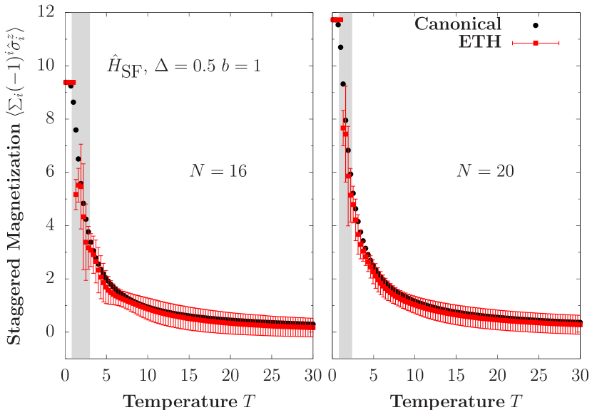
Figure 1: Expectation value of the staggered magnetization as a function of temperature in both the canonical ensemble and the corresponding ETH prediction for and $N=16$ (left) $N=20$ (right). Gray area highlights the low temperature regime, close to the edges of the spectrum where the ETH prediction gives the largest fluctuations.

To evaluate our results in the canonical ensemble and in the context of ETH, we proceed with the full diagonalization of $\hat{H}_{\textrm{SF}}$ in the largest $U(1)$ sector, in which $\sum_{i}\langle\hat{\sigma}^{z}_{i}\rangle=0$. We focus on the total staggered magnetization $\hat{O}=\sum_{i}(-1)^{i}\hat{\sigma}^{z}_{i}$ as our extensive observable, and compute all the matrix elements of $\hat{O}$ in the eigenbasis of the Hamiltonian $\hat{H}_{\textrm{SF}}$ (see SM for an evaluation on a local, non-extensive observable).

Our starting point is to evaluate the expectation value of $\hat{O}$ in the canonical ensemble and compare it with the ETH prediction. In the thermodynamic limit, a single eigenstate $|E\rangle$ with energy $E$ suffices to obtain the canonical prediction: $\langle\hat{O}\rangle=\langle E|\hat{O}|E\rangle{=}\text{Tr}(\hat{O}\,e^{-\beta\hat{H}})/Z$, with an inverse temperature $\beta$ that yields an average energy $E$. For finite-size systems, we instead focus on a small energy window centered around $E$ of width $0.1\epsilon$ in order to average eigenstate fluctuations, where $\epsilon$ is the bandwidth of the Hamiltonian for a given $N$. Fig. 1 shows $\langle\hat{O}\rangle$ as a function of temperature for two different system sizes, including $N=20$, the largest system we have access to (Hilbert space dimension $\mathcal{D}=N!/[(N/2)!(N/2)!]=184\;756$). The results exhibit the expected behavior predicted from ETH for finite-size systems: the thermal expectation value is well approximated away from the edges of the spectrum (low temperature, section highlighted in gray on Fig. 1), and, moreover, the canonical expectation value is better approximated as the system size increases.

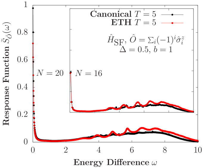
Figure 2: Response function $S_{\hat{O}}(\omega)$ computed directly from ETH and in the canonical ensemble for $N=16$ (inset) and $N=20$ (main) for $T=5$.

We now turn to the evaluation of $\mathcal{F}_{\textrm{ETH}}$ and $\mathcal{F}_{\textrm{Gibbs}}$. The task requires to either compute $S_{\hat{O}}(E,\omega)$ or $\chi^{\prime\prime}_{\hat{O}}(E,\omega)$ in each respective framework. For the former, in the context of ETH, we can employ Eq. (2) which depends only on $f_{\hat{O}}(E,\omega)$. As before, we focus on a small window of energies and extract all the relevant off-diagonal elements of $\hat{O}$ in the eigenbasis of $\hat{H}_{\textrm{SF}}$. Fluctuations are then accounted for by computing a bin average over small windows $\delta\omega$, chosen such that the resulting average produces a smooth curve [see SM for a detailed description on the extraction of $e^{-S(E)/2}f_{\hat{O}}(E,\omega)$] Mondaini and Rigol (2017); Khatami et al. (2013). The procedure leads to a smooth function $e^{-S(E)/2}f_{\hat{O}}(E,\omega)$, in which the first factor is a constant value with respect to $\omega$. The entropy factor can be left undetermined in our calculations if we normalize the curve by the sum rule shown in Eq. (7), computed in this case from the ETH prediction of the expectation value of $\langle\Delta\hat{O}^{2}\rangle$. In the context of the canonical ensemble, $S_{\hat{O}}(\omega)$ can be explicitly evaluated by computing the thermal expectation value of the non-equal correlation function in the frequency domain SM .

In Fig. 2 we show $S_{\hat{O}}(\omega)$ for both the canonical ensemble for $T=5$ and the corresponding ETH prediction normalized by the sum rule mentioned before. The sum rule is evaluated from the expectation values computed within both the canonical ensemble and ETH, correspondingly. It can be observed that the main features of the response function can be well approximated from the corresponding ETH calculation. For this particular case, however, the approximation is only marginally improved by increasing the system size. This behavior is expected given that overall fluctuations for extensive observables carry an extensive energy fluctuation contribution, as mentioned before D’Alessio et al. (2016).

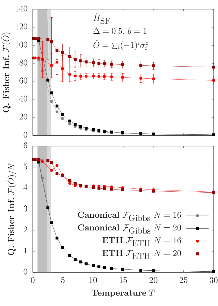
Figure 3: The quantum Fisher information and the corresponding density for different system sizes as a function of temperature in both the canonical ensemble ($\mathcal{F}_{\textrm{Gibbs}}$) and corresponding ETH prediction ($\mathcal{F}_{\textrm{ETH}}$). At infinite temperature ETH predicts the presence of multipartite entanglement while there is none in the canonical ensemble.

The previous analysis unravels the agreement between the thermal expectation values of non-equal correlation functions in time and those predicted by ETH. From these results, as $S_{\hat{O}}(\omega)$ (and, consequently, $\chi^{\prime\prime}_{\hat{O}}(\omega)$ from the FDT) is well approximated by means of ETH, the inequality in Eq. (8) is satisfied.

Finally, we compute the QFI for $\hat{O}$ in our model within both contexts: $\mathcal{F}_{\textrm{ETH}}$ and $\mathcal{F}_{\textrm{Gibbs}}$. The results are shown in Fig. 3. The fluctuations in the ETH calculation of $\mathcal{F}_{\textrm{ETH}}$ are inherited from the fluctuations of the predicted expectation value of $\langle\Delta\hat{O}^{2}\rangle$, which, as expected for finite-size systems, decrease away from the edges of the spectrum. Both predictions for the QFI, canonical and ETH, are equivalent at vanishing temperatures. Remarkably, the QFI predicted from ETH is finite at infinite temperature, while the QFI from the canonical ensemble in this regime vanishes. We emphasize that although the QFI can be used in order to infer the structure of multipartite entanglement i.e. the number of sub-systems entangled, it is not a measure of these correlations (in the mathematical sense of the formal theory of entanglement Horodecki et al. (2009)).

Conclusions.— We have shown that the QFI detects the difference between a pure state satisfying ETH and the Gibbs ensemble at the corresponding temperature. The extension of these results to integrable systems, described by the generalized Gibbs ensemble, is the subject of current work. Even though it is expected that global observables could be sensitive to the difference between pure states and the Gibbs ensemble Garrison and Grover (2018), several operators including sum of local ones and the non-local entanglement entropy appear to coincide at the leading order with the thermodynamic values when ETH is applied Garrison and Grover (2018); Polkovnikov (2011); Santos et al. (2011); Gurarie (2013); Alba and Calabrese (2017). In this work, the difference between ETH/Gibbs multipartite entanglement, which can be macroscopic in proximity of a thermal phase transition, is observed numerically in a XXZ chain with integrability breaking term, when the temperature grows toward infinity. The consequences of this could be observed in ion trap and cold-atom experiments via phase estimation protocols on pure state preparations evolved beyond the coherence time SM . Our result suggests that although at a local level all thermal states look the same, a quantum information perspective indicates that there are many ways to be thermal.

Acknowledgments.— We are grateful to R. Fazio, M. Fabrizio, G. Guarnieri, M. T. Mitchison, L. Pezzè, A. Purkayastha, M. Rigol and A. Smerzi for useful discussions. We thank P. Calabrese, C. Murthy and A. Polkovnikov for the useful comments on the manuscript. M.B. and J.G. acknowledge the DJEI/DES/SFI/HEA Irish Centre for High-End Computing (ICHEC) for the provision of computational facilities and support, project TCPHY104B, and the Trinity Centre for High-Performance Computing. This work was supported by a SFI-Royal Society University Research Fellowship (J.G.) and the Royal Society (M.B.). We acknowledge funding from European Research Council Starting Grant ODYSSEY (Grant Agreement No. 758403).

References

- Gallavotti (2013) G. Gallavotti, Statistical mechanics: A short treatise (Springer Science & Business Media, 2013).
- Schrödinger (1927) E. Schrödinger, Annalen der Physik 388, 956 (1927).
- Neumann (1929) J. v. Neumann, Zeitschrift für Physik 57, 30 (1929).
- Goldstein et al. (2010) S. Goldstein, J. L. Lebowitz, C. Mastrodonato, R. Tumulka, and N. Zanghì, Proceedings of the Royal Society of London A: Mathematical, Physical and Engineering Sciences 466, 3203 (2010).
- Berry and Tabor (1977) M. Berry and M. Tabor, Proceedings of the Royal Society of London A: Mathematical, Physical and Engineering Sciences 356, 375 (1977).
- Berry (1977) M. V. Berry, Journal of Physics A: Mathematical and General 10, 2083 (1977).
- Deutsch (1991) J. M. Deutsch, Physical Review A 43, 2046 (1991).
- Srednicki (1994) M. Srednicki, Physical Review E 50, 888 (1994).
- Srednicki (1996) M. Srednicki, Journal of Physics A: Mathematical and General 29, L75 (1996).
- Srednicki (1999) M. Srednicki, Journal of Physics A: Mathematical and General 32, 1163 (1999).
- Rigol et al. (2008) M. Rigol, V. Dunjko, and M. Olshanii, Nature 452, 854 (2008).
- Polkovnikov et al. (2011) A. Polkovnikov, K. Sengupta, A. Silva, and M. Vengalattore, Reviews of Modern Physics 83, 863 (2011).
- D’Alessio et al. (2016) L. D’Alessio, Y. Kafri, A. Polkovnikov, and M. Rigol, Advances in Physics 65, 239 (2016).
- Kinoshita et al. (2006) T. Kinoshita, T. Wenger, and D. S. Weiss, Nature 440, 900 (2006).
- Lewenstein et al. (2007) M. Lewenstein, A. Sanpera, V. Ahufinger, B. Damski, A. Sen, and U. Sen, Advances in Physics 56, 243 (2007).
- Bloch et al. (2012) I. Bloch, J. Dalibard, and S. Nascimbene, Nature Physics 8, 267 (2012).
- Kitaev (2015) A. Kitaev, “Hidden Correlations in the Hawking Radiation and Thermal Noise (2:00),” https://www.youtube.com/watch?v=OQ9qN8j7EZI (2015).
- Larkin and Ovchinnikov (1969) A. Larkin and Y. N. Ovchinnikov, Sov Phys JETP 28, 1200 (1969).
- Foini and Kurchan (2019) L. Foini and J. Kurchan, Physical Review E 99, 042139 (2019).
- Chan et al. (2019) A. Chan, A. De Luca, and J. T. Chalker, Phys. Rev. Lett. 122, 220601 (2019).
- Helstrom (1969) C. W. Helstrom, Journal of Statistical Physics 1, 231 (1969).
- Tóth and Apellaniz (2014) G. Tóth and I. Apellaniz, Journal of Physics A: Mathematical and Theoretical 47, 424006 (2014).
- Pezze and Smerzi (2014) L. Pezze and A. Smerzi, arXiv preprint arXiv:1411.5164 (2014).
- Giovannetti et al. (2011) V. Giovannetti, S. Lloyd, and L. Maccone, Nature Photonics 5, 222 (2011).
- Pezzè et al. (2018) L. Pezzè, A. Smerzi, M. K. Oberthaler, R. Schmied, and P. Treutlein, Reviews of Modern Physics 90 (2018).
- Hyllus et al. (2012) P. Hyllus, W. Laskowski, R. Krischek, C. Schwemmer, W. Wieczorek, H. Weinfurter, L. Pezzé, and A. Smerzi, Physical Review A 85 (2012).
- Tóth (2012) G. Tóth, Physical Review A 85 (2012).
- Hauke et al. (2016) P. Hauke, M. Heyl, L. Tagliacozzo, and P. Zoller, Nature Physics 12, 778 (2016).
- Gabbrielli et al. (2018) M. Gabbrielli, A. Smerzi, and L. Pezzè, Scientific Reports 8 (2018).
- Frérot and Roscilde (2018) I. Frérot and T. Roscilde, Physical Review Letters 121, 020402 (2018).
- Deutsch et al. (2013) J. M. Deutsch, H. Li, and A. Sharma, Physical Review E 87 (2013).
- Vidmar and Rigol (2017) L. Vidmar and M. Rigol, Physical Review Letters 119, 220603 (2017).
- Murthy and Srednicki (2019a) C. Murthy and M. Srednicki, Physical Review E 100, 022131 (2019a).
- Braunstein and Caves (1994) S. L. Braunstein and C. M. Caves, Physical Review Letters 72, 3439 (1994).
- Petz and Ghinea (2011) D. Petz and C. Ghinea, in Quantum Probability and Related Topics (World Scientific, 2011).
- Pezzè et al. (2017) L. Pezzè, M. Gabbrielli, L. Lepori, and A. Smerzi, Physical Review Letters 119, 250401 (2017).
- (37) Since the definition (5) applies to both the microcanonical (MC) and the canonical Gibbs ensembles, if the energy width of the two coincide, then the QFI’s are the same and given exactly by Eq.(6). See the SM for a derivation based on the ETH. From now on we assume equivalence of ensembles, otherwise only the microcanonical result should be considered.
- (38) The long-time average of a time-dependent function is defined as . In the case of two-times functions , than the time-average is performed over the average time .
- Rossini et al. (2014) D. Rossini, R. Fazio, V. Giovannetti, and A. Silva, EPL (Europhysics Letters) 107, 30002 (2014).
- Pappalardi et al. (2017) S. Pappalardi, A. Russomanno, A. Silva, and R. Fazio, Journal of Statistical Mechanics: Theory and Experiment 2017, 053104 (2017).
- (41) See the Supplemental Material at [] for additional information about the extraction of , numerical details, results on a local non-extensive observable, a short review regarding the asymptotic Quantum Fisher Information after quenched dynamics and the validity of the fluctuation-dissipation theorem within ETH and the possible experimental consequences of our result. The Supplemental Material contains Refs. Mondaini and Rigol (2017); D’Alessio et al. (2016); Beugeling et al. (2015); Mukerjee et al. (2006); Murthy and Srednicki (2019b); Rossini et al. (2014); Pappalardi et al. (2017); Hauke et al. (2016); Pezzè et al. (2018); Paris (2009).
- (42) Since in standard thermodynamics energy fluctuations are small , the same expansion around the average energy done for the diagonal ensemble can be performed for , therefore .
- Cardy (2012) J. Cardy, Finite-size scaling, Vol. 2 (Elsevier, 2012).
- Brenes et al. (2018) M. Brenes, E. Mascarenhas, M. Rigol, and J. Goold, Physical Review B 98, 235128 (2018).
- Mondaini and Rigol (2017) R. Mondaini and M. Rigol, Physical Review E 96, 012157 (2017).
- Khatami et al. (2013) E. Khatami, G. Pupillo, M. Srednicki, and M. Rigol, Physical Review Letters 111, 050403 (2013).
- Horodecki et al. (2009) R. Horodecki, P. Horodecki, M. Horodecki, and K. Horodecki, Rev. Mod. Phys. 81, 865 (2009).
- Garrison and Grover (2018) J. R. Garrison and T. Grover, Phys. Rev. X 8, 021026 (2018).
- Polkovnikov (2011) A. Polkovnikov, Annals of Physics 326, 486 (2011).
- Santos et al. (2011) L. F. Santos, A. Polkovnikov, and M. Rigol, Physical Review Letters 107, 040601 (2011).
- Gurarie (2013) V. Gurarie, Journal of Statistical Mechanics: Theory and Experiment 2013, P02014 (2013).
- Alba and Calabrese (2017) V. Alba and P. Calabrese, Physical Review B 96, 115421 (2017).
- Beugeling et al. (2015) W. Beugeling, R. Moessner, and M. Haque, Phys. Rev. E 91, 012144 (2015).
- Mukerjee et al. (2006) S. Mukerjee, V. Oganesyan, and D. Huse, Phys. Rev. B 73, 035113 (2006).
- Murthy and Srednicki (2019b) C. Murthy and M. Srednicki, arXiv preprint arXiv:1906.10808 (2019b).
- Paris (2009) M. G. Paris, International Journal of Quantum Information 7, 125 (2009).