Parallel Computation of Graph Embeddings

Abstract

Graph embedding aims at learning a vector-based representation of vertices that incorporates the structure of the graph. This representation then enables inference of graph properties. Existing graph embedding techniques, however, do not scale well to large graphs. We therefore propose a framework for parallel computation of a graph embedding using a cluster of compute nodes with resource constraints. We show how to distribute any existing embedding technique by first splitting a graph for any given set of constrained compute nodes and then reconciling the embedding spaces derived for these subgraphs. We also propose a new way to evaluate the quality of graph embeddings that is independent of a specific inference task. Based thereon, we give a formal bound on the difference between the embeddings derived by centralised and parallel computation. Experimental results illustrate that our approach for parallel computation scales well, while largely maintaining the embedding quality.

1 Introduction

Graphs are a natural representation of relations between entities in complex systems, such as social networks or information networks. To enable inference on graphs, a graph embedding may be learned. It comprises vertex embeddings, each being a vector-based representation of a graph’s vertex that incorporates its relations with other vertices (?). Inference tasks, such as vertex classification and link prediction, can then be based on the graph embedding rather than the original graph. Various techniques to learn a graph embedding have been proposed (?; ?; ?). However, common techniques aim at high embedding quality at the expense of computational efficiency, so that they do not scale to extremely large graphs that comprise billions of nodes and trillions of edges (?). Computing an embedding with traditional techniques for graphs of such sizes may take weeks, which renders it practically infeasible. Moreover, such computations are challenging in terms of their memory requirements. For example, storing a graph with two billion nodes in main memory requires around 1TB RAM (?), which exceeds the capacity of commodity servers.

Against this background, we argue that graph embedding shall exploit parallel computation in a cluster of compute nodes. However, the parallelisation of graph embedding is challenging for various reasons.

First, a graph shall be split into subgraphs, each of which is processed separately by a compute node. This is difficult, since compute nodes have resource constraints. Their memory capacity is limited, which induces a bound on the size of any subgraph that can be handled by a node. Any split of the graph thus needs to incorporate these resource constraints.

A second challenge is the reconciliation of embeddings computed for subgraphs. Each node learns an embedding for only a subset of graph vertices, so that the results are vectors in different embedding spaces. An alignment of these spaces is needed to obtain a meaningful graph embedding.

The need to reconcile embedding spaces leads to a third challenge, i.e., the evaluation of the quality of a graph embedding. Traditionally, embedding quality is assessed based on some inference task, such as vertex classification or link prediction. However, such an approach renders the measurement dependent on a specific task, which precludes a general assessment of how the quality of embeddings is affected by parallel computation and subsequent reconciliation.

In this paper, we answer these challenges in a unifying framework. We provide a method to decompose a graph, such that the resulting subgraphs satisfy resource constraints imposed by compute nodes. These subgraphs share some vertices, called anchors, that facilitate reconciliation of the derived embeddings. Intuitively, the differences in the embeddings of an anchor as part of different subgraphs guide the alignment of the respective embedding spaces. We show how to select such anchors effectively in order to minimise the impact of the parallel computation on the embedding quality. To assess this effect, we adopt the idea of the Pairwise Inner Product (PIP) (?; ?), a loss metric proposed for word embedding tasks, and propose a way to measure embedding quality in an intrinsic manner. Based thereon, we give a theoretical bound on the difference between a graph embedding derived by centralised computation and our parallelization scheme. Comprehensive experiments with real-world data illustrate the effectiveness and efficiency of our approach.

In the remainder, Section 2 first gives an overview of our approach. Section 3 then outlines how to embed subgraphs, while Section 4 focuses on reconciliation of embedding spaces. Section 5 presents a measure to compare embeddings, which is used for a theoretical analysis in Section 6. Experimental results are presented in Section 7. Section 8 reviews related work, before we conclude in Section 9.

2 Parallel Graph Embedding Framework

2.1 Computational Model

Let $G=(V,E)$ be an undirected graph with vertices $V$ and edges $E\subseteq[V]^{2}$. A graph embedding technique aims to learn a mapping $f:V\rightarrow\mathcal{R}^{d}$ from vertices $V$ to an embedding in a low-dimensional space ($d\ll|V|$), such that ‘similar’ vertices are mapped to close vertex embeddings (?). The similarity of vertices may, e.g., be measured based on the ratio of common neighbouring vertices or the similarity of vertex labels. Closeness of two vertex embeddings, in turn, is commonly measured by their cosine similarity. Typically, the mapping $f$ is parameterised, so that the graph embedding problem is to find parameters of $f$ that minimise the difference between the similarity assigned to vertices and the closeness of their respective embeddings.

Traditional techniques focus on optimising the quality of a graph embedding, which limits their scalability. Learning embeddings for large graphs comes with a large memory footprint, while training times may extend to days or even weeks (?). We therefore aim to parallelise the computation of a graph embedding in a cluster of $n$ compute nodes. In a cluster, each such node has resource constraints in terms of the available memory and runtime. Here, we focus on memory constraints, since runtime requirements directly depend on the size of the graph and, hence, the required memory to store the graph. Specifically, we denote by $k_{1},\ldots,k_{n}$ the memory constraints of $n$ compute nodes and assume that they are expressed as the maximal size of the graph that can be handled, i.e., the $i$-th node may process a graph with up to $k_{i}$ vertices.

2.2 Problem Statement

To parallelise the computation of a graph embedding, the following problem needs to be addressed:

Problem 1.

Let $G=(V,E)$ be a graph and $f$ a reference embedding technique, so that $f(G)=\mathbf{E}$. Given a cluster of $n$ nodes with memory constraints $k_{1},\ldots,k_{n}$, the problem of parallel graph embedding is to devise an embedding technique $f_{d}$, $f_{d}(G)=\mathbf{F}$, that exploits the $n$ nodes, satisfies the memory constraints of all nodes, and minimises the difference between $\mathbf{F}$ and $\mathbf{E}$.

Here, we assume that $\sum_{1\leq i\leq n}k_{i}>|V|$. As a reference embedding technique, we consider techniques for centralised computation of graph embeddings, such as DeepWalk (?), HOPE (?), and SGC (?). These techniques are representative methods for the three main approaches to graph embedding, which are grounded in random-walks, matrix factorisation, and graph neural networks, respectively.

2.3 Approach

Our general idea is to split a graph into $n$ subgraphs, so that the computation of the vertex embeddings can be parallelised among $n$ compute nodes. Then, the memory constraint $k_{i}$ of the $i$-th node gives a bound for the size of the $i$-th subgraph. However, the vertex embeddings computed per subgraph are of different spaces. Our approach therefore is to construct subgraphs that share some vertices, called anchors, which enable us to reconcile the embedding spaces.

A realisation of this idea is challenging, though. There is an exponential number of possible decompositions of a graph into $n$ partially overlapping subgraphs. Each split has different consequences for the quality of the reconciled embedding. To minimise the difference between the graph embeddings obtained by centralised and parallel computation, an effective strategy for the selection of anchors is needed.

Figure 1: Framework for parallel computation of graph embeddings on distributed nodes with resource constraints.

Given the above considerations, we propose a graph embedding framework, shown in Figure 1, as follows:

• First, we decompose the graph into subgraphs and select a set of anchors. Given the importance of anchors for reconciliation of embedding spaces, we present an effective selection strategy in Section 3.

• Once a graph is decomposed into $n$ subgraphs, we learn an embedding per subgraph on a separate compute node. As our framework is agnostic to the chosen embedding algorithm, it improves scalability of any existing graph embedding technique.

• In this step, we reconcile the embedding spaces obtained for different subgraphs on different compute nodes by constructing a function that maps from one embedding space to another one. We show how to construct such a mapping in Section 4.

As stated in Problem 1, we strive for a minimal distance between the graph embedding obtained with centralised computation, $\mathbf{E}$, and the one derived by parallel computation, $\mathbf{F}$. We therefore also clarify how to evaluate embeddings independent of a specific inference task (Section 5) and give a bound for the difference between centralised and parallel computation of graph embeddings (Section 6).

3 Decomposition for Subgraph Embedding

We first outline requirements on the graph decomposition for parallel embedding. We then present a strategy for anchor selection, before discussing the embedding of subgraphs.

3.1 Graph Decomposition

While graph decomposition is a well-studied problem, there are several requirements that pertain to our setting. First, subgraph sizes shall be proportional to the memory constraints of compute nodes. Second, the number of edges between non-anchor vertices shall be minimised, as these edges are neglected when embedding the subgraphs. Formally, a graph decomposition is a function that takes a graph $G$, the number of subgraphs $n$, and the maximal subgraph sizes $\{k_{1},\ldots,k_{n}\}$ as input, and returns a set of subgraphs, $\mathit{decompose}(G,n,\{k_{1},\ldots,k_{n}\})=\{P_{1},\ldots,P_{n}\}$, where $P_{i}=(V_{i},E_{i})$ is a subgraph of $G$. Here, we leverage METIS (?) to decompose a graph. It is a scalable algorithm for unbalanced decomposition, i.e., it incorporates constraints on maximal subgraph sizes.

3.2 Anchor Selection

Several criteria shall be considered when devising a strategy to select a set of anchors $A\subseteq V$ for the subgraphs of a graph $G=(V,E)$. The number of anchors $|A|$ has a great effect on the ability to reconcile the embeddings computed for different subgraphs. A large number of anchors provides many clues for reconciliation and, thus, is expected to lead to higher overall embedding quality. On the other hand, a large number of anchors is problematic, as the respective vertex embeddings are computed several times. As such, there is a trade-off between the ability to reconcile embedding spaces (i.e., the goodness of the mapping between the spaces) and the overall required learning effort. Moreover, the structural importance of anchors influences the reconciliation of embedding spaces. A higher anchor connectivity yields a better alignment of the dimensions of embedding spaces.

Against this background, we propose to select anchors by exploiting properties of the decomposition of the graph. Given the set of vertices that are part of subgraph borders, denoted by $U\subseteq V$, we select a set of anchors $A\subseteq U$ based on vertex connectivity. That is, we select the top-$d$ nodes in $U$ that have the highest number of edges between subgraphs. The intuition is that by selecting these vertices, we are able to reduce the number of edges that are removed by the decomposition and anchor selection process.

input : Graph $G=(V,E)$; number of subgraphs $n$; number of anchors $d$;
maximal subgraph sizes $\{k_{1},\ldots,k_{n}\}$.

output :  $n$ subgraphs $P_{1},\ldots,P_{n}$; anchors $A$.

// Graph decomposition

1 $(V_{1},E_{1}),...,(V_{n},E_{n})=\mathit{decomp}(G,n,\{k_{1},...,k_{n}\})$;

// Select anchors

2 $C=\{\{u,v\}\in E\mid u\in V_{i}\wedge v\in V_{j}\wedge i\neq j\}$;

3 $L=\{\{u,h_{u}\}\mid h_{u}=\sum_{v\in V}\mathds{1}_{\{u,v\}\in C}\}$;

4 $A=select\_top(L,d)$;

// Merge with anchors

5 for $i\in[1,n]$ do

6      

$$P_{i}=(V_{i}\cup A,\{\{u,v\}\mid\{u,v\}\in E\ \wedge\\ u\in V_{i}\cup A\ \wedge\ v\in V_{i}\cup C\})$$

7return $P_{1},\ldots,P_{n},A$;

Algorithm 1 Graph decomposition for embedding.

This strategy is formalised in Algorithm 1. The algorithm first decomposes the graph $G$ into $n$ subgraphs that satisfy the size constraints $\{k_{1},\ldots,k_{n}\}$ (line 1). We then consider the border vertices of the resulting subgraphs (line 1) and select the $d$ vertices with the highest numbers of edges (line 1) as anchors. The anchors are added to the subgraphs (line 1), before returning the subgraphs and anchors.

3.3 Subgraph Embedding

Given the subgraphs $P_{1},\ldots,P_{n}$ generated above, we leverage any existing graph embedding technique for the subgraphs. A reference embedding procedure $f$ embeds each subgraph $P_{i}$, which yields a matrix $\mathbf{F}_{i}$ of vertex embeddings. The resulting embedding spaces represented by these matrices tend to differ for any two subgraphs. However, since the subgraphs share anchors, it is possible to reconcile the embedding spaces.

4 Reconciling Embedding Spaces

To reconcile embeddings that have been constructed independently of each other, one may either construct a pairwise mapping between any two spaces, or map all of them into one pivot space. The former has to cope with a combinatorial blow-up of the number of required mappings. Reconciliation with a pivot space, in turn, requires the joint construction of $n$ mappings, with $n$ being the number of subgraphs.

Regardless of the above design choice, our idea is to reconcile embedding spaces based on anchors. An anchor will be associated with different embeddings in different embedding spaces, even though it relates to the same entity, i.e., the same vertex in the original graph. Hence, anchors tell us how to convert an embedding space into another one.

Figure 2 shows embedding spaces derived for two subgraphs, where embeddings of three anchors are shown as stars, triangles, and squares. By ‘rotating’ one embedding space, such that the embeddings of anchors in either spaces are close to each other, we are able to align the two spaces.

Figure 2: Reconciliation of embedding spaces.

Assume that we decomposed a graph $G$ into subgraphs $P_{1},\ldots,P_{n}$ and obtained the embeddings $\mathbf{F}_{1},\ldots,\mathbf{F}_{n}$ for these subgraphs. We strive for a mapping of embeddings $\mathbf{F}_{1},\ldots,\mathbf{F}_{n}$ into a single embedding space, which, without loss of generality, is one of the $n$ spaces, denoted by $\mathbf{F}_{0}$. We propose to learn a mapping function $h(\mathbf{F}_{i})$ that takes a source embedding space as input and returns a mapped space, such that the embeddings of the anchors are close in $\mathbf{F}_{0}$. This approach is inspired by techniques for network alignment (?) and cross-lingual dictionary building (?; ?). The mapping function can be linear or a multilayer perceptron (?). In any case, our objective is captured by the following loss function:

$$L(h,\mathbf{F}_{i},\mathbf{F}_{0},A)=\sum_{v\in A}||h(\mathbf{z}_{i,v})-\mathbf{z}_{0,v}||_{F}$$ (1)

where $||.||_{F}$ is the Frobenius norm, $A$ is the set of anchors, and $\mathbf{z}_{i,v}$ is the embedding of anchor $v$ in $\mathbf{F}_{i}$. Since it was shown that a linear function is sufficient to obtain a good mapping (?; ?), we define the mapping function as $h(\mathbf{F}_{i})=\mathbf{F}_{i}\times\mathbf{W}$ where $\mathbf{W}\in\mathcal{R}^{d\times d}$ and $d$ is the embedding dimensionality. The above equation is rewritten in its matrix form, if we denote the embedding matrices of the anchor nodes of $\mathbf{F}_{i}$ and $\mathbf{F}_{0}$ as $\mathbf{H}_{i}$ and $\mathbf{H}_{0}$:

$$L(\mathbf{H}_{i},\mathbf{H}_{0},\mathbf{W})=||\mathbf{H}_{i}\mathbf{W}-\mathbf{H}_{0}||_{F}$$

Furthermore, it is known that a better mapping is obtained when enforcing orthogonality on $\mathbf{W}$ (?). Under the orthogonality constraint, the mapping matrix $\mathbf{W}$ that minimises Eq. 1 is found using singular value decomposition (SVD). Let $\mathbf{U}\mathbf{\Sigma}\mathbf{V}^{T}=\mathbf{H}_{0}\mathbf{H}_{i}^{T}$ be the SVD of the matrix $\mathbf{H}_{0}\mathbf{H}_{i}^{T}$. Then, $\mathbf{W}$ is computed as $\mathbf{W}=\mathbf{U}\mathbf{V}^{T}$.

While we focus on mapping the anchors, the learned mapping function is applicable to the whole embedding space. In other words, let $\mathbf{W}_{i}$ be the mapping matrix from $\mathbf{H}_{i}$ to $\mathbf{H}_{0}$. Then, the reconciled embedding space of $\mathbf{F}_{i}$ is $\mathbf{F}_{i}\mathbf{W}_{i}$.

5 Evaluating Embeddings

Having introduced our framework for parallel graph embedding, we turn to the evaluation of embeddings. Specifically, we assess if and how much an embedding $\mathbf{E}$ derived by centralised computation differs from an embedding $\mathbf{F}$ derived by parallel computation. Note that for such a comparison, embedding $\mathbf{F}$ is constructed from the reconciled embeddings obtained for the subgraphs, as explained above: Given the reconciled spaces $\mathbf{F}_{1}\mathbf{W}_{1},\ldots,\mathbf{F}_{n}\mathbf{W}_{n},\mathbf{F}_{0}$, we concatenate the matrices and reorder rows (vertex embeddings), so that the row order (vertex order) is similar to the one in $\mathbf{E}$.

5.1 Extrinsic Evaluation

Extrinsic evaluation measures the quality of embeddings based on some downstream inference tasks. For instance, in vertex classification, an embedding is used to assign class labels to vertices after a learning process. Hence, metrics for classification quality, such as accuracy, can be used to indirectly quantify the difference between two embeddings. Such an approach introduces a bias, though, since the inference task may be influenced by various factors. For instance, in vertex classification, the quality of the classifier and the correctness of the labels may have a dramatic impact. Even if the embedding quality is high (it captures the structural relations of vertices), the classification accuracy may be low, if the vertex labels are incorrect.

5.2 Intrinsic Evaluation

We therefore propose to compare embeddings solely based on their intrinsic properties. Given two embedding matrices $\mathbf{Z}_{1}$ and $\mathbf{Z}_{2}$ of the same set of vertices $V$, as the matrices represent vertex embeddings, the difference between $\mathbf{Z}_{1}$ and $\mathbf{Z}_{2}$ is traced back to the difference between embeddings of a vertex $u$: $\mathbf{z}_{1,u}\in\mathbf{Z}_{1}$ and $\mathbf{z}_{2,u}\in\mathbf{Z}_{2}$. Note though, that the absolute value of $u$’s embeddings has no meaning: If $\mathbf{z}_{1,u}$ and $\mathbf{z}_{2,u}$ differ, they are simply different representations of the same entity. However, we can exploit that a graph embedding aims to preserve the vertex similarity in the graph. Hence, if vertex $v$ is similar to $u$ in the graph, the embeddings of $v$ and $u$ shall be close. In other words, the distance between $\mathbf{z}_{1,v}$ and $\mathbf{z}_{1,u}$ and the distance between $\mathbf{z}_{2,v}$ and $\mathbf{z}_{2,u}$ should be similar: Both $\mathbf{z}_{1,u}$ and $\mathbf{z}_{2,u}$ are embeddings of $u$, while $\mathbf{z}_{1,v}$ and $\mathbf{z}_{2,v}$ are embeddings of $v$.

The above means that the similarity between $\mathbf{z}_{1,u}$ and $\mathbf{z}_{2,u}$ may be revealed in comparison to other vertices’ embeddings. Let $L=(c_{1},\ldots,c_{l})$ be a set of ‘core’ vertices. Then, the difference between $\mathbf{z}_{1,u}$ and $\mathbf{z}_{2,u}$ is measured based on their distance with the embeddings of the core vertices:

$$d(\mathbf{z}_{1,u},\mathbf{z}_{2,u}|L)=||(\mathbf{z}_{1,u}\mathbf{z}^{T}_{1,c_{1}},\ldots,\mathbf{z}_{1,u}\mathbf{z}^{T}_{1,c_{l}})-\\ (\mathbf{z}_{2,u}\mathbf{z}^{T}_{2,c_{1}},\ldots,\mathbf{z}_{2,u}\mathbf{z}^{T}_{2,c_{l}})||_{F}$$ (2)

where $\mathbf{z}_{1,u}\mathbf{z}^{T}_{1,c_{1}}$ is the inner product. Based thereon, we can compute the difference between two embedding spaces $\mathbf{Z}_{1}$ and $\mathbf{Z}_{2}$ based on the difference in embeddings of each vertex $u\in V$. Considering all vertices as ‘core’ vertices ($L=V$), we obtain the PIP metric as defined for word embedding tasks (?; ?):

$$PIP(\mathbf{Z}_{1},\mathbf{Z}_{2})=||\mathbf{Z}_{1}\mathbf{Z}_{1}^{T}-\mathbf{Z}_{2}\mathbf{Z}_{2}^{T}||_{F}.$$

The smaller the obtained value, the more similar are the two embedding spaces.

6 Theoretical Bounds

Next, we analyse the difference between an embedding obtained with centralised computation, $\mathbf{E}$, and the one obtained by parallel computation, $\mathbf{F}$, using the above metric. We first discuss how graph embedding can be considered as a form of matrix factorisation, before providing a bound for the aforementioned difference.

6.1 Graph Embedding as Matrix Factorisation

Most graph embedding techniques are implicit matrix factorisations (?; ?) of a signal matrix $\mathbf{M}$ that can be constructed from the adjacency matrix $\mathbf{A}$. Graph embedding techniques differ in how they construct the signal matrix (?). For instance, the LINE embedding technique (?) aims to factorise the matrix $\mathbf{M}=({1}/{vol(G)})\mathbf{C}^{-1}\mathbf{A}\mathbf{C}^{-1}$,where $\mathbf{C}$ is the degree diagonal matrix and $vol(G)$ is the sum of all vertex degrees. Another example is the signal matrix of HOPE (?), which is $\mathbf{M}=\mathbf{A}\mathbf{A}$.

Given a signal matrix $\mathbf{M}$ and its SVD $\mathbf{M}=\mathbf{U}\mathbf{D}\mathbf{V}$, an embedding is constructed by $\mathbf{E}=\mathbf{U}_{.,1:k}\mathbf{D}_{1:k,1:k}^{\alpha}$ with $\alpha\in[0,1]$ as a signal parameter and $k$ as the embedding dimensionality.

6.2 Bound for Parallel Computation

For simplicity, we assume that the graph is decomposed into two non-overlapping subgraphs of size $n_{1}$ and $n_{2}$. The assumption of a non-overlapping split does not affect our analysis, since the PIP metric is agnostic to the application of an orthogonal mapping matrix $\mathbf{E}\mathbf{E}^{T}=(\mathbf{EW})(\mathbf{EW})^{T}$.

Theorem 1.

Let $\mathbf{E}$ and $\mathbf{F}$ be embeddings derived by centralised and parallel computation, respectively. The PIP distance between $\mathbf{E}$ and $\mathbf{F}$ is bounded:

$$PIP(\mathbf{E},\mathbf{F})\leq 3\sum_{i=1}^{k}\lambda_{i}^{2\alpha}+2\sum_{i=1}^{k}(\lambda_{i}^{2\alpha}-\lambda_{i+1}^{2\alpha})\sqrt{i(n-i)}+\\ +\sum_{m\in\{n_{1},n_{2}\}}\sqrt{\sum_{i=1}^{2m-n}(\lambda_{i}^{2\alpha}-\lambda_{i+2(n-m)}^{2\alpha})^{2}+\sum_{i=2m-n+1}^{k}\lambda_{i}^{4\alpha}}$$ (3)

where $\lambda_{i}$ is the $i$-th singular value of the signal matrix $\mathbf{M}$ and $\alpha$ is the signal parameter.

To prove Theorem 1, we need the following lemmas.

Lemma 1.

Let $\lambda_{i}$ be the $i$-th singular value of a signal matrix $\mathbf{M}$ and $\lambda^{\prime}_{i}$ be the $i$-th singular value of a signal matrix $\mathbf{M}^{\prime}$, where $\mathbf{M}^{\prime}$ is the submatrix of $\mathbf{M}$. Then, it holds that:

$$\sqrt{\sum_{i=1}^{k}(\lambda_{i}^{2\alpha}-\lambda_{i}^{\prime 2\alpha})}\leq\sqrt{\sum_{i=1}^{2m-n}(\lambda_{i}^{2\alpha}-\lambda_{i+2(n-m)}^{2\alpha})^{2}+\Theta}$$

where $\Theta=\sum_{i=2m-n+1}^{k}\lambda_{i}^{4\alpha}$.

Lemma 2.

With $\lambda_{i}$, $\lambda^{\prime}_{i}$, $\mathbf{M}$, and $\mathbf{M}^{\prime}$ as defined in Lemma 1, it holds that:

$$\sqrt{\sum_{i}^{k}\lambda_{i}^{\prime 2\alpha}}\leq\sum_{i=1}^{k}\lambda_{i}^{2\alpha}$$

Both lemmas follow directly from the properties of singular values of submatrices, see (?). Using these results, we prove Theorem 1 as follows:

Proof.

Let $\mathbf{F}_{1},\mathbf{F}_{2}$ be the embeddings of the two subgraphs from which $\mathbf{F}$ has been derived. Let further $\mathbf{E}_{1},\mathbf{E}_{2}$ be the corresponding partial embeddings from $\mathbf{E}$. This means that $\mathbf{E}$ is the embedding derived by decomposing the signal matrix $\mathbf{M}$, while $\mathbf{M}_{1}$ and $\mathbf{M}_{2}$ are the signal matrices of the two subgraphs that generate $\mathbf{F}_{1},\mathbf{F}_{2}$. In other words, $\mathbf{F}_{1}=\mathbf{Y}\mathbf{D}_{1}^{\alpha},\mathbf{F}_{2}=\mathbf{Z}\mathbf{D}_{2}^{\alpha}$ and $\mathbf{E}_{i}=\mathbf{X}_{i}\mathbf{D}^{\alpha}$. In addition, $\mathbf{M}_{1},\mathbf{M}_{2}$ are the submatrices of $\mathbf{M}$. We also have:

$$PIP(\mathbf{E},\mathbf{F})=PIP(\mathbf{E}_{1},\mathbf{F}_{1})+PIP(\mathbf{E}_{2},\mathbf{F}_{2})\\ +||\mathbf{E}_{1}\mathbf{E}_{2}^{T}-\mathbf{F}_{1}\mathbf{F}_{2}^{T}||+||\mathbf{E}_{2}\mathbf{E}_{1}^{T}-\mathbf{F}_{2}\mathbf{F}_{1}^{T}||$$ (4)

We bound the terms on the right-hand side of the above equation using Theorem 2 in (?):

$$PIP(\mathbf{E}_{1},\mathbf{F}_{1})+PIP(\mathbf{E}_{2},\mathbf{F}_{2})\leq\sum_{j\in\{1,2\}}\sqrt{\sum_{i=1}^{k}(\lambda_{i}^{2\alpha}-\lambda_{i}^{(j)2\alpha})}\\ +\sqrt{2}\sum_{i=1}^{k}(\lambda_{i}^{2\alpha}-\lambda_{i+1}^{2\alpha})(||\mathbf{Y}_{.,1:i}^{T}\mathbf{X}_{.,i:n}^{(1)}||+||\mathbf{Z}_{.,1:i}^{T}\mathbf{X}_{.,i:n}^{(2)}||)$$ (5)

The first term can be further bounded using Lemma 1. The term $||\mathbf{Y}_{.,1:i}^{T}\mathbf{X}_{.,i:n}^{(1)}||+||\mathbf{Z}_{.,1:i}^{T}\mathbf{X}_{.,i:n}^{(2)}||$ is bounded as follows:

$$||\mathbf{Y}_{.,1:i}^{T}\mathbf{X}_{.,i:n}^{(1)}||+||\mathbf{Z}_{.,1:i}^{T}\mathbf{X}_{.,i:n}^{(2)}||\leq\\ ||\mathbf{Y}_{.,1:i}^{T}||||\mathbf{X}_{.,i:n}^{(1)}||+||\mathbf{Z}_{.,1:i}^{T}||||\mathbf{X}_{.,i:n}^{(2)}||\\ \leq\sqrt{i}(||\mathbf{X}_{.,i:n}^{(1)}||+||\mathbf{X}_{.,i:n}^{(2)}||)\leq\sqrt{i}\sqrt{2(||\mathbf{X}_{.,i:n}^{(1)}||^{2}+||\mathbf{X}_{.,i:n}^{(2)}||^{2})}\\ \leq\sqrt{i}\sqrt{2(n-i)}\leq\sqrt{2i(n-i)}$$ (6)

The next to last term in Eq. 4 is bounded as follows:

$$||\mathbf{E}_{1}\mathbf{E}_{2}^{T}-\mathbf{F}_{1}\mathbf{F}_{2}^{T}||\leq||\mathbf{E}_{1}\mathbf{E}_{2}^{T}||+||\mathbf{F}_{1}\mathbf{F}_{2}^{T}||\\ \leq||\mathbf{E}_{1}||||\mathbf{E}_{2}^{T}||+||\mathbf{F}_{1}||||\mathbf{F}_{2}^{T}||\\ \leq\frac{1}{2}(||\mathbf{E}_{1}||^{2}+||\mathbf{E}_{2}^{T}||^{2})+||\mathbf{F}_{1}||||\mathbf{F}_{2}^{T}||\\ \leq\frac{1}{2}\sum_{i}^{k}\lambda_{i}^{2\alpha}+\sqrt{\sum^{k}_{i=1}\lambda^{(1)2\alpha}_{i}}\sqrt{\sum^{k}_{i=1}\lambda^{(2)2\alpha}_{i}}$$ (7)

We obtain a similar bound for the last term in Eq. 4. Combining the above equations, the last two terms in Equation 4 are bounded as follows:

$$||\mathbf{E}_{1}\mathbf{E}_{2}^{T}-\mathbf{F}_{1}\mathbf{F}_{2}^{T}||+||\mathbf{E}_{2}\mathbf{E}_{1}^{T}-\mathbf{F}_{2}\mathbf{F}_{1}^{T}||\leq\\ \sum_{i}^{k}\lambda_{i}^{2\alpha}+2\sqrt{\sum^{k}_{i=1}\lambda^{(1)2\alpha}_{i}\sum^{k}_{i=1}\lambda^{(2)2\alpha}_{i}}\leq\sum_{i}^{k}\lambda_{i}^{2\alpha}+2\sum_{i=1}^{k}\lambda_{i}^{2\alpha}$$ (8)

where we use Lemma 2 in the last inequality. Combining Equation 4, 5 and 8, we obtain Theorem 1. ∎

Theorem 1 shows that the PIP distance between embeddings derived by centralised and parallel computation is bounded only by the singular values of the original signal matrix and a chosen embedding size. Hence, while there are different ways to decompose a graph, the quality of the resulting embedding is bounded by the graph structure.

7 Empirical evaluation

7.1 Experimental setup

Datasets. We evaluate our approach to parallel computation of graph embeddings using several datasets (Table 1) in different tasks. For the task of vertex classification, we use BlogCatalog (?), a social network of blog authors, in which labels capture topics, and Flickr (?), a network of users on a photo sharing website where labels represent user groups having the same interest. For the task of link prediction, we consider Arxiv (?), a collaboration graph of scientist, and Youtube , a network of Youtube users. To evaluate the scalability of our proposed method, we rely on LiveJournal (?), an online blogging network of user friendships, and Wikipedia (?), a dataset containing hyperlinks from Wikipedia articles. In total, the LiveJournal dataset contains nearly 40 million edges and nodes, while the Wikipedia dataset contains more than 25 million edges and nodes. All datasets are publicly available.

Metrics. We measure the efficiency of parallel computation of graph embeddings and the embedding quality. For our framework, learning time is measured as the maximum embedding time on each compute node and the maximum time required to reconcile two embedding spaces. The memory requirement is measured in the same vein. The embedding quality is assessed indirectly, as the F1-score in vertex classification, and ROC and AP scores in link prediction. A direct quality metric is the PIP distance between the embeddings derived by centralised and parallel computation (see Section 5.2), normalized by the number of graph vertices.

7.2 Efficiency

We first explore the gains in efficiency that result from our approach to parallel computation. We compare our framework with PBG (?), which is the only existing technique to distribute graph embedding to a set of compute nodes. Unlike our approach, however, PBG assumes that compute nodes share storage and communicate during training. To achieve a fair comparison, we disable such communication among nodes when running PBG. Also, note that PBG is inherently limited to edge-based embedding techniques.

We increase the number of compute nodes (and, thus, subgraphs) from 2 to 10 for our largest datasets (Livejournal and Wikipedia), selecting 1% of the vertices as anchors. This decreases learning time significantly. For instance, we achieve a time speedup of 6.9 with eight compute nodes in comparison with only 5.1 for PBG on the Livejournal dataset (Figure 5). Our approach outperforms PBG constantly in term of speedup as we increase the number of compute nodes. In addition, from Figure 5, we observe that the quality of the embeddings remains nearly the same as the level of parallelism increases. On the other hand, the embedding quality of PBG decreases significantly as more compute nodes are used. For instance, while the difference in micro-f1 score between our approach and PBG is only 0.016 when 2 compute nodes are used, it becomes 0.137 with 10 compute nodes, which is a nearly 9$\times$ increase. We can explain this observation based on the reference embedding method. Since PBG is restricted to an edge-based embedding method, its embedding quality is more susceptible to partitioning. In this experiment, however, we rely on DeepWalk as the reference embedding method, which alleviates the above problem: Random walks allow to connect subgraphs from their common anchors.

Table 1: Datasets statistics

Dataset	# Vertices	# Edges
BlogCatalog	10’312	333’983
Flickr	80’513	5’899’882
Arxiv	18’722	198’110
Youtube	495’957	1’936’748
Wikipedia	1’791’489	28’511’807
LiveJournal	3’997’962	34’681’189

Figure 3: Time speedup

Figure 4: Memory speedup

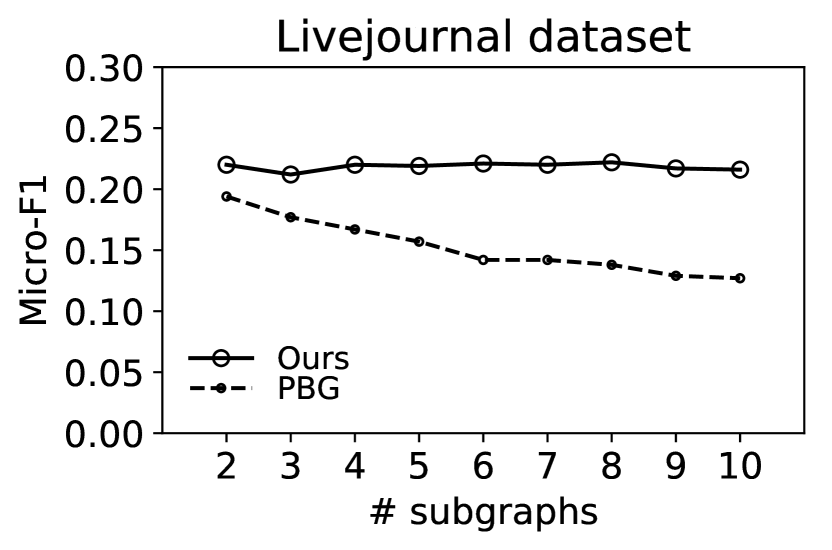
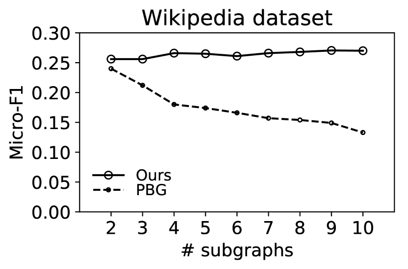
Figure 5: Effects of parallelism on performance.

Table 2: Our framework against different embedding techniques (micro-F1). Similar trends hold for macro-F1.

	BlogCatalog			Flickr
	DW	HOPE	SGN	DW	HOPE	SGN
NoRecon	0.272	0.238	0.231	0.365	0.271	0.282
Recon-R	0.272	0.245	0.238	0.367	0.290	0.281
Recon-S	0.284	0.242	0.246	0.384	0.298	0.29

Table 3: PIP distance to the centralised embeddings (the lower, the better).

	BlogCatalog			Flickr
	DW	HOPE	SGN	DW	HOPE	SGN
NoRecon	1.55	18.6	0.42	17.06	157.42	3.12
Recon-R	1.08	10.57	0.38	10.31	67.11	2.65
Recon-S	1.102	9.45	0.35	9.52	38.21	2.77

7.3 Ablation Studies

Next, we compare the quality of embeddings generated by our framework and its variants, i.e., with and without reconciliation; and using a random or our proposed anchor selection strategy. We denote our framework with the proposed anchor selection as Recon-S, with random anchor selection as Recon-R. We also consider a variant where no reconciliation is used (NoRecon). In addition, we analyse the effects of the embedding method on the embedding quality. Here, we consider three embedding methods (DeepWalk (?), HOPE (?), and SGN (?)) that represent the state-of-the-art for the three main classes of approaches for graph embedding (walk-based, matrix factorization, and graph neural network).

Table 4: Effects of embedding strategies on link prediction.

	arxiv						youtube
	DW		HOPE		SGN		DW		HOPE		SGN
	ROC	AP	ROC	AP	ROC	AP	ROC	AP	ROC	AP	ROC	AP
D	0.843	0.883	0.890	0.926	0.827	0.877	0.822	0.845	0.813	0.880	0.622	0.699
DAB	0.808	0.856	0.887	0.924	0.815	0.898	0.749	0.776	0.810	0.876	0.641	0.706
DAS	0.878	0.899	0.918	0.94	0.857	0.901	0.831	0.842	0.843	0.896	0.662	0.729

Vertex Classification. We report the classification accuracy (Table 3) and the PIP metric (Table 3). We observe that our proposed reconciliation mechanism turns out to be effective, improving the embedding quality in nearly all settings. For instance, the F1 score for the Flickr dataset using the DeepWalk embedding technique without reconciliation is 0.365, while it is 0.384 when reconciliation is used. The effect of reconciliation is also seen in Table 3: The differences in PIP distance between the embeddings with centralised computation are smaller for the reconciled embeddings (Recon-R, Recon-S) than for the non-reconciled ones (NoRecon). Moreover, our anchor selection strategy (Recon-S) provides better embeddings across different datasets and techniques in comparison with the baseline strategy (Recon-S).

Link prediction. To evaluate our approach in the context of link prediction, we remove 50% of the edges from the graphs, and use the embeddings to predict the removed edges. We select the same amount of vertex pairs that have no link in the original graphs as negative samples. The obtained results, see Table 4, confirm the observations obtained for vertex classification. Our framework consistently outperforms the baseline strategies. For instance, reconciliation improves the ROC and AP scores (dataset Arxiv, embedding technique DeepWalk) from 0.843 and 0.883 to 0.878 and 0.899, respectively.

8 Related Work

Graph representation learning aims to construct a low-dimensional model of the vertices in the graph that incorporates the graph structure (?; ?). Existing techniques differ in how they map a vertex into an embedding space, and in the structural properties that shall be retained. There are three main approaches to embed a vertex, using shallow or deep encoders (?), or matrix factorisation. Techniques that use shallow encoders (?; ?) consider vertices as words and random walks as sentences, which allows them to use neural word embedding techniques such as word2vec (?) to construct word/vertex embeddings. On the other hand, deep encoder approaches such as GraphSAGE (?) or SGN (?) consider the neighbourhood of a vertex to generate its embedding. As a consequence, both vertex features and the graph structure may be captured.

There are recent works that aim to scale traditional graph embedding methods to very large graphs. MILE (?) aims to scale traditional graph embedding techniques to large graph using only one workstation. A large graph is coarsened into a small one and embedding is performed on the small graph. This approach does not try to leverage a set of compute nodes, though. Closest to our work is PBG (?), which aims to learn embeddings in a distributed manner. As mentioned earlier, PBG assumes a different setting compared to our approach. PBG has been proposed for compute nodes with shared storage that also communicate during training, whereas we focus on a shared-nothing infrastructure, as it is commonly encountered in compute clusters. A second major difference is that PBG is tailored to scale shallow embedding methods that use negative sampling to large graphs. Our framework, in turn, allows to scale any embedding technique and is, therefore, more generally applicable. In particular, it can be combined with deep approaches, such as GraphSAGE and SGN, which suffer from long training times in practice.

9 Conclusion

In this paper, we took on the challenge of scaling arbitrary graph embedding techniques to very large graphs, using a cluster of compute nodes. We showed how to decompose a graph for distributed computation, taking into account the resource constraints of a given set of compute nodes. We then proposed a mechanism to reconcile the embeddings obtained independently for the individual subgraphs and also contributed a way to assess embedding quality, independent of a specific inference task. Using this measure, we gave formal guarantees on the difference between embeddings derived by centralised and parallel computation. Experiments showed that our approach is efficient and effective: It scales well, largely maintains the embedding quality, and consistently outperforms the sole existing approach to exploit a cluster of compute nodes for graph embedding.

References

- [Artetxe et al. 2016] Mikel Artetxe, Gorka Labaka, and Eneko Agirre. Learning principled bilingual mappings of word embeddings while preserving monolingual invariance. In EMNLP, pages 2289–2294, 2016.
- [Cai et al. 2018] Hongyun Cai, Vincent W Zheng, and Kevin Chang. A comprehensive survey of graph embedding: problems, techniques and applications. TKDE, 2018.
- [Conneau et al. 2018] Alexis Conneau, Guillaume Lample, Marc’Aurelio Ranzato, Ludovic Denoyer, and Hervé Jégou. Word translation without parallel data. ICLR, 2018.
- [Grover and Leskovec 2016] Aditya Grover and Jure Leskovec. node2vec: Scalable feature learning for networks. In KDD, pages 855–864, 2016.
- [Hamilton et al. 2017a] Will Hamilton, Zhitao Ying, and Jure Leskovec. Inductive representation learning on large graphs. In NIPS, pages 1024–1034, 2017.
- [Hamilton et al. 2017b] William L Hamilton, Rex Ying, and Jure Leskovec. Representation learning on graphs: Methods and applications. IEEE Data Engineering Bulletin, 2017.
- [Karypis and Kumar 1998] George Karypis and Vipin Kumar. A software package for partitioning unstructured graphs, partitioning meshes, and computing fill-reducing orderings of sparse matrices. University of Minnesota, Department of Computer Science and Engineering, Army HPC Research Center, Minneapolis, MN, 1998.
- [Lerer et al. 2019] Adam Lerer, Ledell Wu, Jiajun Shen, Timothee Lacroix, Luca Wehrstedt, Abhijit Bose, and Alex Peysakhovich. Pytorch-biggraph: A large-scale graph embedding system. arXiv preprint arXiv:1903.12287, 2019.
- [Leskovec et al. 2007] Jure Leskovec, Jon Kleinberg, and Christos Faloutsos. Graph evolution: Densification and shrinking diameters. ACM Transactions on Knowledge Discovery from Data (TKDD), 1(1):2, 2007.
- [Liang et al. 2018] Jiongqian Liang, Saket Gurukar, and Srinivasan Parthasarathy. Mile: A multi-level framework for scalable graph embedding. arXiv preprint arXiv:1802.09612, 2018.
- [Liu et al. 2019] Xin Liu, Tsuyoshi Murata, Kyoung-Sook Kim, Chatchawan Kotarasu, and Chenyi Zhuang. A general view for network embedding as matrix factorization. In Proceedings of the Twelfth ACM International Conference on Web Search and Data Mining, pages 375–383. ACM, 2019.
- [Man et al. 2016] Tong Man, Huawei Shen, Shenghua Liu, Xiaolong Jin, and Xueqi Cheng. Predict anchor links across social networks via an embedding approach. In IJCAI, pages 1823–1829, 2016.
- [Mikolov et al. 2013] Tomas Mikolov, Kai Chen, Greg Corrado, and Jeffrey Dean. Efficient estimation of word representations in vector space. arXiv preprint arXiv:1301.3781, 2013.
- [Ou et al. 2016] Mingdong Ou, Peng Cui, Jian Pei, Ziwei Zhang, and Wenwu Zhu. Asymmetric transitivity preserving graph embedding. In Proceedings of the 22nd ACM SIGKDD international conference on Knowledge discovery and data mining, pages 1105–1114. ACM, 2016.
- [Perozzi et al. 2014] Bryan Perozzi, Rami Al-Rfou, and Steven Skiena. Deepwalk: Online learning of social representations. In KDD, pages 701–710, 2014.
- [Qiu et al. 2018] Jiezhong Qiu, Yuxiao Dong, Hao Ma, Jian Li, Kuansan Wang, and Jie Tang. Network embedding as matrix factorization: Unifying deepwalk, line, pte, and node2vec. In Proceedings of the Eleventh ACM International Conference on Web Search and Data Mining, pages 459–467. ACM, 2018.
- [Ruck et al. 1990] Dennis W Ruck, Steven K Rogers, Matthew Kabrisky, Mark E Oxley, and Bruce W Suter. The multilayer perceptron as an approximation to a bayes optimal discriminant function. IEEE Transactions on Neural Networks, 1(4):296–298, 1990.
- [Tang and Liu 2009] Lei Tang and Huan Liu. Relational learning via latent social dimensions. In Proceedings of the 15th ACM SIGKDD international conference on Knowledge discovery and data mining, pages 817–826. ACM, 2009.
- [Tang et al. 2015] Jian Tang, Meng Qu, Mingzhe Wang, Ming Zhang, Jun Yan, and Qiaozhu Mei. Line: Large-scale information network embedding. In Proceedings of the 24th International Conference on World Wide Web, pages 1067–1077. International World Wide Web Conferences Steering Committee, 2015.
- [Thompson 1972] ROBERT C Thompson. Principal submatrices ix: Interlacing inequalities for singular values of submatrices. Linear Algebra and its Applications, 5(1):1–12, 1972.
- [Wu et al. 2019] Felix Wu, Amauri Souza, Tianyi Zhang, Christopher Fifty, Tao Yu, and Kilian Weinberger. Simplifying graph convolutional networks. In International Conference on Machine Learning, pages 6861–6871, 2019.
- [Yang and Leskovec 2015] Jaewon Yang and Jure Leskovec. Defining and evaluating network communities based on ground-truth. Knowledge and Information Systems, 42(1):181–213, 2015.
- [Yin and Shen 2018] Zi Yin and Yuanyuan Shen. On the dimensionality of word embedding. In Advances in Neural Information Processing Systems, 2018.
- [Yin et al. 2017] Hao Yin, Austin R Benson, Jure Leskovec, and David F Gleich. Local higher-order graph clustering. In Proceedings of the 23rd ACM SIGKDD International Conference on Knowledge Discovery and Data Mining, pages 555–564. ACM, 2017.
- [Yin et al. 2018] Zi Yin, Vin Sachidananda, and Balaji Prabhakar. The global anchor method for quantifying linguistic shifts and domain adaptation. In Advances in Neural Information Processing Systems, pages 9434–9445, 2018.