Scalings Pertaining to Current Sheet Disruption Mediated by the Plasmoid Instability

Abstract

Analytic scaling relations are derived for a phenomenological model of the plasmoid instability in an evolving current sheet, including the effects of reconnection outflow. Two scenarios are considered, where the plasmoid instability can be triggered either by an injected initial perturbation or by the natural noise of the system (here referred to as the system noise). The two scenarios lead to different scaling relations because the initial noise decays when the linear growth of the plasmoid instability is not sufficiently fast to overcome the advection loss caused by the reconnection outflow, whereas the system noise represents the lowest level of fluctuations in the system. The leading order approximation for the current sheet width at disruption takes the form of a power law multiplied by a logarithmic factor, and from that, the scaling relations for the wavenumber and the linear growth rate of the dominant mode are obtained. When the effects of the outflow are neglected, the scaling relations agree, up to the leading order approximation, with previously derived scaling relations based on a principle of least time. The analytic scaling relations are validated with numerical solutions of the model.

I Introduction

Thin current sheets, which appear to be ubiquitous in laboratory, space, and astrophysical plasmas, are known to be unstable to the plasmoid instability,(Biskamp, 1986; Loureiro et al., 2007; Bhattacharjee et al., 2009) which disrupts current sheets to form smaller structures such as plasmoids (or flux ropes) and secondary current sheets. Plasmoid-instability-mediated disruption of reconnecting current sheets plays a crucial role in triggering the transition from slow to fast magnetic reconnection,(Bhattacharjee et al., 2009; Daughton et al., 2009; Cassak et al., 2009; Huang and Bhattacharjee, 2010; Shepherd and Cassak, 2010; Huang et al., 2011, 2017) and also modifies the energy cascade in magnetohydrodynamic (MHD) turbulence, making the energy power spectrum steeper than predicted by traditional MHD turbulence theories.(Carbone et al., 1990; Huang and Bhattacharjee, 2016; Mallet et al., 2017; Loureiro and Boldyrev, 2016; Boldyrev and Loureiro, 2017; Comisso et al., 2018; Dong et al., 2018; Walker et al., 2018)

In early theoretical studies of the plasmoid instability, it was commonly assumed that the aspect ratio of the current sheet follows the Sweet-Parker scaling $L/a\simeq\sqrt{S}$,(Parker, 1957; Sweet, 1958) where $S\equiv LV_{A}/\eta$ is the Lundquist number. Here, $L$ and $a$ denote the half-length and the half-width of the current sheet, respectively, $V_{A}$ is the Alfvén speed, and $\eta$ is the magnetic diffusivity. For resistive magnetohydrodynamics (MHD) model, this assumption yields the scaling relations $\gamma\sim S^{1/4}$ for the linear growth rate and $k\sim S^{3/8}$ for the wavenumber of the fastest growing mode.(Tajima and Shibata, 1997; Loureiro et al., 2007; Bhattacharjee et al., 2009) Following the same assumption, scaling relations have also been derived for other models, including Hall MHD(Baalrud et al., 2011) and visco-resistive MHD.(Comisso and Grasso, 2016)

However, a current sheet in nature typically forms dynamically, starting from a broader sheet that gradually thins down. The fact that the Sweet-Parker-based scaling $\gamma\sim S^{1/4}$ diverges in the asymptotic limit of $S\to\infty$ indicates that for a high-$S$ current sheet, the disruption may occur before the current sheet realizes the Sweet-Parker aspect ratio.(Pucci and Velli, 2014) The precise conditions for current sheet disruption have been a topic of active research in recent literature.(Pucci and Velli, 2014; Tenerani et al., 2015, 2016; Uzdensky and Loureiro, 2016; Comisso et al., 2016, 2017; Huang et al., 2017; Tolman et al., 2018) By using a principle of least time, Comisso et al. showed that the current sheet width, the linear growth rate, and the dominant mode wavenumber at disruption do not follow power-law scaling relations.(Comisso et al., 2016, 2017) Huang et al. proposed a phenomenological model incorporating the effects of reconnection outflow.(Huang et al., 2017) Numerical solutions of this model have been extensively tested with results from direct numerical simulations.

The objective of this work is to develop a methodology to obtain analytic scaling relations for the phenomenological model of Huang et al. for a special class of evolving current sheets, which is modeled by a Harris sheet thinning down exponentially in time, where the upstream magnetic field remains constant. This paper is organized as follows. Section II gives an overview of the model. Section III gives a formal solution of the model equation based on the method of characteristics. The solution is then applied in Section IV to obtain scaling relations for key features at the disruption time, such as the current sheet width, the linear growth rate, and the dominant mode wavenumber. Here, we consider two possible scenarios. In the first scenario, an initial noise is injected into the system to trigger the plasmoid instability. In the second scenario, the plasmoid instability evolves from the natural noise of the system, referred to as the “system noise” in this paper. The two scenarios lead to different scaling relations because the initial noise tends to decay during an early time when the linear growth of the plasmoid instability is not sufficiently fast to overcome the advection loss caused by the reconnection outflow; on the other hand, the system noise represents the lowest level of fluctuations pertaining to the system even when no external noise is injected. In Section V, we consider the case where the effects of the outflow are neglected. In this case, we show that the scaling relations agree with that of Comisso et al. up to the leading order approximation. We also validate the analytic scaling relations by comparing them with numerical solutions. We conclude in Section VI.

II Phenomenological Model

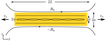
Figure 1: Schematic diagram of the plasmoid instability in a reconnecting current sheet. Here, the shaded area is the current sheet of a length $2L$ and a width $2a$. The length and width can both be functions of time. The magnetic fields immediately outside the current sheet are $\pm B_{x}$, and the reconnection outflow speed is $v_{o}$. Within the current sheet are two additional length scales: the inner layer width $2\delta$, and the magnetic island width $2w$. Current sheet disruption occurs when the magnetic island width exceeds the inner layer width.

In this Section, we give a brief outline of the phenomenological model. The reader is referred to Ref. [Huang et al., 2017] for the details of the derivation. Figure 1 shows a schematic diagram for the system we consider here. The following equation governs the linear phase of the plasmoid instability in an evolving current sheet:

$$\partial_{t}f-k\frac{v_{o}}{L}\partial_{k}f=\left(\gamma-\frac{v_{o}}{2L}+\frac{1}{2L}\frac{dL}{dt}\right)f.$$ (1)

Here, $f(k,t)\equiv|\hat{B}_{z}(k,t)|/B_{0}L_{0}$ is the Fourier amplitude of the magnetic field fluctuation normal to the current sheet as a function of the wavenumber $k$ and the time $t$, normalized to the characteristic magnetic field $B_{0}$ and length $L_{0}$ of the system, $v_{o}$ is the outflow speed, $\gamma(k,t)$ is the linear growth rate of the tearing instability, and $L$ is the half-length of the current sheet. Here, the linear growth rate $\gamma$ explicitly depends on time because the current sheet can evolve in time. The differential operator in the left-hand-side incorporates the stretching effect on wavelength due to the reconnection outflow; the right-hand-side represents the effects of linear growth, advection loss due to the outflow, and evolution of the current sheet length. The domain of wavenumber $k$ is limited to $k\geq\pi/L$ because the wavelength must be smaller than the current sheet length $2L$.

The linear growth rate $\gamma(k,t)$ depends on the profile of magnetic field $B_{x}(z,t)$, which can be a function of time depending on the system under consideration. The model also allows the current sheet half-length $L$ to change in time, as represented by the $(1/2L)dL/dt$ term. The outflow speed $v_{0}$ can also be time-dependent. To integrate the model equation, we need $\gamma(k,t)$, $v_{o}(t)$, $L(t)$, and an initial condition $f=f_{0}(k)$ as inputs. With these conditions provided, we can integrate equation (1) in time until the plasmoid instability enters the nonlinear regime, which occurs when the typical half-width $w$ of plasmoids exceeds the inner layer half-width $\delta$. At that moment, the fluctuating part of the current density $\tilde{J}$ is of the same order of the background current density $J$, implying that the current sheet has lost its integrity. Therefore, we take $w=\delta$ as the condition for current sheet disruption.

This condition for current sheet disruption depends critically on the half-width $w$ of plasmoids. However, the precise definition of $w$ is nuanced. The nuance comes from the fact that while $w$ is well-defined when the magnetic fluctuation $\tilde{B}$ is a single-mode Fourier harmonic (as is often assumed in tearing mode analyses), it is not so when the fluctuation is a superposition of a continuum of Fourier modes. In this model problem, fortunately, a meaningful half-width $w$ of plasmoids can be defined because, as we will see, the solution $f$ typically becomes localized around a dominant wavenumber $k_{d}$ as time progresses. For a spectrum $f(k)$ localized around $k=k_{d}$, we define the plasmoid half-width $w$ as

$$w=2\sqrt{\frac{\tilde{B}}{k_{d}B_{x}^{\prime}}},$$ (2)

where the prime denotes $d/dz$ evaluated at $z=0$. In Eq. (2), the fluctuation amplitude $\tilde{B}$ must take into account the contribution from all the neighboring modes of the dominant mode. Precisely, a superposition of all the modes in the range $k\in[k_{d}/\xi,k_{d}\xi]$ gives a fluctuation amplitude

$$\tilde{B}=\left(\frac{L_{0}^{2}}{\pi L}\int_{k_{d}/\xi}^{k_{d}\xi}f(k^{\prime})^{2}dk^{\prime}\right)^{1/2}B_{0}.$$ (3)

Here, the $O(1)$ parameter $\xi$ sets the range of superposition. As the Fourier spectrum $f(k)$ is usually well-localized at the disruption time, the amplitude $\tilde{B}$ is insensitive to the choice of $\xi$, provided that $\xi$ is not too close to unity (e.g., $\xi=1.5$ was used in Ref. [Huang et al., 2017]). Note that for a single-mode perturbation, the definition (2) reduces to the usual expression for magnetic island half-width.(Biskamp, 1993)

The plasmoid half-width $w$ must be compared with the inner layer half-width $\delta$ to determine the condition for current sheet disruption. As the inner layer half-width $\delta$ depends on the wavenumber, we adopt the inner layer half-width at the dominant wavenumber $k_{d}$ for this comparison. For resistive tearing modes we consider in this study, the inner layer half-width for $k=k_{d}$ is given by

$$\delta=\left(\frac{\eta\,\gamma(k_{d})}{\left(k_{d}V_{A}\right)^{\prime 2}}\right)^{1/4},$$ (4)

where $\eta$ is the magnetic diffusivity. Here, the prime again denotes $d/dz$ evaluated at $z=0$, and $V_{A}$ is the Alfvén speed of the reconnecting component $B_{x}$. The criterion $w=\delta$, with $w$ and $\delta$ defined by Eqs. (2–4), then determines the condition for current sheet disruption. This criterion has been extensively tested and validated with numerical simulations.(Huang et al., 2017)

III Integral Solution of the Model Equation for a thinning Harris Sheet

Up to now, the model is general regarding the time evolution of both the current sheet profile and the reconnection outflow. To fix ideas and make the model analytically tractable, we assume that the current sheet can be modeled by a Harris sheet and the time evolution of the width $a$ obeys the form

$$a^{2}=a_{\infty}^{2}+(a_{0}^{2}-a_{\infty}^{2})\exp(-2t/\tau).$$ (5)

In this form, assuming $a_{\infty}\ll a_{0}$, the current sheet width $a$ decreases exponentially at early times with $a\simeq a_{0}e^{-t/\tau}$, and $a\to a_{\infty}$ as $t\to\infty$. We further assume that the upstream magnetic field $B_{x}$ and the current sheet half-length $L$ remain fixed in time and that the outflow speed $v_{o}$ is the upstream Alfvén speed $V_{A}$. Under these conditions, if the plasmoid instability does not disrupt the current sheet, eventually the current sheet will approach the Sweet-Parker current sheet, which is a steady-state solution of reconnection governed by resistive MHD. Therefore, we set the asymptotic half-width $a_{\infty}$ to be the Sweet-Parker width, i.e., $a_{\infty}=L/\sqrt{S}$, where $S\equiv LV_{A}/\eta$ is the Lundquist number. These assumptions are consistent with direct numerical simulations reported in Ref. [Huang et al., 2017]. Heuristic derivations for Eq. (5) can be found in Refs. [Kulsrud, 2005] and [Huang et al., 2017].

Under the assumption that the upstream $B_{x}$ and the current sheet length $L$ are fixed in time, it is natural to choose $B_{0}=B_{x}$ and $L_{0}=L$ as the characteristic magnetic field and length scale. Hereafter, we normalize lengths and times with respect to the current sheet half-length $L$ and the Alfvén time $\tau_{A}\equiv L/V_{A}$, as follows: $\hat{t}=t/\tau_{A}$, $\hat{\tau}=\tau/\tau_{A}$, $\hat{k}=kL$, $\hat{a}=a/L$, and $\hat{\gamma}=\gamma\tau_{A}$. The model equation in normalized variables is

$$\partial_{\hat{t}}f-\hat{k}\partial_{\hat{k}}f=\left(\hat{\gamma}-\frac{1}{2}\right)f,$$ (6)

where $dL/dt=0$ is assumed.

We can solve Eq. (6) by the method of characteristics. The characteristic starting from $\hat{k}=\hat{k}_{0}$ at $\hat{t}=\hat{t}_{0}$ is given by

$$\hat{k}\left(\hat{t};\hat{k}_{0},\hat{t}_{0}\right)=\hat{k}_{0}e^{-(\hat{t}-\hat{t}_{0})},$$ (7)

which represents the mode-stretching effect due to the reconnection outflow. Now the differential operator on the left-hand-side of Eq. (6) is simply the time derivative along characteristics and hence the solution can be obtained by integrating along them, yielding

$$f(\hat{k},\hat{t})=f(\hat{k}_{0},\hat{t}_{0})\exp\left[\int_{\hat{t}_{0}}^{\hat{t}}\hat{\gamma}\left(\hat{k}(\hat{t}^{\prime}),\hat{t}^{\prime}\right)d\hat{t}^{\prime}-\frac{\hat{t}-\hat{t}_{0}}{2}\right].$$ (8)

To perform the integration, we need the linear growth rate $\hat{\gamma}$ as a function of the wavenumber and time. The linear growth rate of the tearing mode is governed by the tearing stability index $\Delta^{\prime}$,(Furth et al., 1963) which depends entirely on the solution of linearized ideal MHD force-free equation in the outer region away from the resonant surface (where $\mathbf{k}\cdot\mathbf{B}=0$). The tearing instability requires the condition $\Delta^{\prime}>0$ being satisfied. While the complete dispersion relation for resistive tearing modes can be expressed in terms of $\Delta^{\prime}$, the expression is involved and requires solving a transcendental equation.(Coppi et al., 1976) Analytically tractable approximations can be obtained in two limits: the small-$\Delta^{\prime}$ regime for short-wavelength modes and the large-$\Delta^{\prime}$ regime for long-wavelength modes. In the small-$\Delta^{\prime}$ regime (large $k$ and $\Delta^{\prime}\delta\ll 1$), the linear growth rate is given by (Furth et al., 1963)

$$\gamma_{s}=C_{\Gamma}\eta^{3/5}(\Delta^{\prime}/2)^{4/5}\left(kV_{A}\right)^{\prime 2/5},$$ (9)

where $C_{\Gamma}=\left(\pi{}^{-1}\Gamma(1/4)/\Gamma(3/4)\right)^{4/5}\approx 0.953$. In the the large-$\Delta^{\prime}$ regime (small $k$ and $\Delta^{\prime}\delta\gg 1$), the linear growth rate is approximately given by (Coppi et al., 1976)

$$\gamma_{l}=\eta^{1/3}\left(kV_{A}\right)^{\prime 2/3}.$$ (10)

Here, the derivative $\left(kV_{A}\right)^{\prime}$ is evaluated at the resonant surface. For a Harris sheet profile with $V_{A}(z)=V_{A}\tanh(z/a)$, the tearing stability index $\Delta^{\prime}$ is given by

$$\Delta^{\prime}=\frac{2}{a}\left(\frac{1}{ka}-ka\right).$$ (11)

From Eqs. (9–11), we obtain the normalized growth rates for a Harris sheet in the small-$\Delta^{\prime}$ regime

$$\hat{\gamma}_{s}=C_{\Gamma}\hat{a}^{-2}S^{-3/5}\hat{k}^{-2/5}(1-\hat{k}^{2}\hat{a}^{2})^{4/5}$$ (12)

and in the large-$\Delta^{\prime}$ regime

$$\hat{\gamma}_{l}=\hat{a}^{-2/3}S^{-1/3}\hat{k}^{2/3}.$$ (13)

The two asymptotic limits (12) and (13) can be smoothly connected by a function

$$\hat{\gamma}=\frac{\hat{\gamma_{s}}\hat{\gamma_{l}}}{\left(\hat{\gamma_{s}}^{\zeta}+\hat{\gamma_{l}}^{\zeta}\right)^{1/\zeta}},$$ (14)

for an arbitrary $\zeta$. In this work, we take the value $\zeta=3/2$, which gives a nearly exact approximation of the true dispersion relation. Furthermore, we will neglect the factor $(1-\hat{k}^{2}\hat{a}^{2})$ in Eq. (12) for our analytic derivations. This approximation can be justified a posteriori by noting that the dominant mode wavenumber $\hat{k}_{d}$ follows the same scaling as the fastest growing mode wavenumber $\hat{k}_{\text{max}}$ [see Eq. (35) and the discussion thereafter] and that $\hat{k}_{\text{max}}\hat{a}\simeq(S\hat{a}){}^{-1/4}$ (see below); therefore, in the high-$S$ regime, the condition $\hat{k}\hat{a}\ll 1$ is satisfied in the neighborhood (in the $k$-space) of the dominant mode, which is our primary interest. Note that, from the scaling of the disruption current sheet width, Eq. (47), the condition $S\hat{a}\gg 1$ is satisfied. Putting these approximations together yields an approximate expression for the linear growth rate that is valid for $\hat{k}\hat{a}\ll 1$, i.e.,

$$\hat{\gamma}\simeq\frac{C_{\Gamma}S^{-3/5}\hat{k}^{-2/5}\hat{a}^{-2}}{\left(1+C_{\Gamma}^{3/2}S^{-2/5}\hat{k}^{-8/5}\hat{a}^{-2}\right)^{2/3}}.$$ (15)

We will apply this expression to Eq. (8) to derive scaling relations in Section IV.

The fastest growing mode occurs at the transition between the small-$\Delta^{\prime}$ and the large-$\Delta^{\prime}$ regimes, i.e., at $\hat{k}\hat{a}\simeq(S\hat{a}){}^{-1/4}$ where $\hat{\gamma}_{s}\simeq\hat{\gamma}_{l}$. More precisely, the fastest growing wavenumber $\hat{k}_{\text{max}}$ is given by (see, e.g., Ref. [Schindler, 2007])

$$\hat{k}_{\text{max}}\approx 1.358\,(S\hat{a}){}^{-1/4}\hat{a}^{-1}$$ (16)

and the corresponding growth rate is

$$\hat{\gamma}_{\text{max}}\approx 0.623\,S^{-1/2}\hat{a}^{-3/2}.$$ (17)

IV Scaling Relations for Current Sheet Disruption

In this Section we derive scaling relations for key features at current sheet disruption in the high-$S$ regime, under the assumptions detailed in Sec. III. Specifically, the disruption time $\hat{t}_{d}$, the current sheet width $\hat{a}_{d}$, the dominant mode wavenumber $\hat{k}_{d}$, and the linear growth rate $\hat{\gamma}_{d}$ of the dominant mode are derived analytically. Here we consider two cases. In the first case, an initial noise is injected into the system. The initial noise is assumed to be much larger than the system noise; therefore the latter is ignored and set to zero in the analysis. In the second case, there is no initial noise, and the system noise is the seed from which the plasmoid instability develops.

IV.1 Case I — Initial Perturbation

Let the initial perturbation be $f_{0}(\hat{k}_{0})$ at $\hat{t}_{0}=0$. To integrate the linear growth rate along a characteristic in Eq. (8), it is convenient to define a new variable

$$\varphi\equiv C_{\Gamma}^{-3/4}S^{1/5}\hat{k}^{4/5}\hat{a}.$$ (18)

In the high-$S$ regime we consider here, it can be shown a posteriori that current sheet disruption occurs when $\hat{a}_{d}\gg\hat{a}_{\infty}$, because $\hat{a}_{d}$ follows a weaker scaling with respect to $S$ [see Eq. (47)] than $\hat{a}_{\infty}$, which is assumed to be the Sweet-Parker width $\hat{a}_{SP}=S^{-1/2}$. Hence, we will ignore $a_{\infty}$ in Eq. (5) and assume $\hat{a}=\hat{a}_{0}e^{-\hat{t}/\hat{\tau}}$ in the following analysis. The combined effect of mode stretching ($\hat{k}=\hat{k}_{0}e^{-(\hat{t}-\hat{t}_{0})}$) and current sheet thinning $(\hat{a}=\hat{a}_{0}e^{-\hat{t}/\hat{\tau}})$ implies that the variable $\varphi$ decreases exponentially in time as

$$\varphi=\varphi_{0}e^{-\hat{t}/\hat{\tau}_{*}},$$ (19)

where the time scale $\hat{\tau}_{*}$ is defined as

$$\hat{\tau}_{*}=\frac{5\hat{\tau}}{4\hat{\tau}+5}.$$ (20)

The linear growth rate, Eq. (15), can be expressed in terms of $\varphi$ instead of $\hat{k}$ as

$$\hat{\gamma}\simeq C_{\Gamma}^{5/8}S^{-1/2}\hat{a}^{-3/2}\frac{\varphi{}^{-1/2}}{\left(1+\varphi^{-2}\right)^{2/3}}.$$ (21)

We can now integrate the growth rate along the characteristic with a change of variable from $\hat{t}$ to $\varphi$, yielding

$$\int_{0}^{\hat{t}}\hat{\gamma}(\hat{k}_{0}e^{-\hat{t}^{\prime}},\hat{t}^{\prime})d\hat{t}^{\prime}$$

$$\simeq -C_{\Gamma}^{5/8}S^{-1/2}\hat{a}^{-3/2}\varphi^{3\hat{\tau}_{*}/2\hat{\tau}}\hat{\tau}_{*}\int_{\varphi_{0}}^{\varphi}\frac{\varphi^{\prime-3/2-3\hat{\tau}_{*}/2\hat{\tau}}}{\left(1+\varphi^{\prime-2}\right)^{2/3}}d\varphi^{\prime}$$

$$= \,\frac{\hat{\tau}_{\sharp}}{2}C_{\Gamma}^{5/8}S^{-1/2}\hat{a}^{-3/2}\varphi^{3\hat{\tau}_{*}/2\hat{\tau}}\left.G(\varphi^{\prime};\hat{\tau})\right|_{\varphi_{0}}^{\varphi},$$ (22)

where

$$G(\varphi^{\prime};\hat{\tau})=\varphi^{\prime-1/2-3\hat{\tau}_{*}/2\hat{\tau}}\,_{2}F_{1}\left(\frac{\hat{\tau}_{*}}{\hat{\tau}_{\sharp}},\frac{2}{3};\frac{\hat{\tau}_{*}}{\hat{\tau}_{\sharp}}+1;-\varphi^{\prime-2}\right).$$ (23)

Here, ${}_{2}F_{1}$ is the hypergeometric function(Abramowitz and Stegun, 1972) and

$$\hat{\tau}_{\sharp}\equiv\frac{4\hat{\tau}\hat{\tau}_{*}}{\hat{\tau}+3\hat{\tau}_{*}}=\dfrac{5\hat{\tau}}{\hat{\tau}+5}.$$ (24)

To proceed from Eq. (22), we further make the approximation that in the high-$S$ regime, the contribution from the lower boundary, $G(\varphi_{0};\hat{\tau})$, is negligible compared to the contribution from the upper boundary, $G(\varphi;\hat{\tau})$, at the disruption time. This approximation can be justified a posteriori using the scaling relation of the disruption current sheet width $\hat{a}_{d}$ in Eq. (47). Because $\hat{a}_{d}$ decreases as $S$ increases, it follows from the relation $\varphi/\varphi_{0}=(\hat{a}/\hat{a}_{0})^{\hat{\tau}/\hat{\tau}_{*}}$ that in the high-$S$ regime, the condition $\varphi\ll\varphi_{0}$ is satisfied at the disruption time, where the variable $\varphi$ is typically an $O(1)$ quantity in the neighborhood of the dominant mode [see the discussion in the paragraph below Eq. (34)]. The function $G(\varphi^{\prime};\hat{\tau})$ is monotonically decreasing with respect to $\varphi^{\prime}$. Its overall behavior is well captured by two asymptotic expressions for small and large $\varphi^{\prime}$, which can be obtained using the asymptotic expansion of the hypergeometric function near $x\to\infty$:

$${}_{2}F_{1}\left(c,b;c+1;-x\right)= \frac{\Gamma(c+1)\Gamma(b-c)}{\Gamma(b)}x^{-c}$$

$$+\frac{c}{c-b}x^{-b}+O\left(x^{-b-1}\right)$$ (25)

and the Taylor expansion near $x=0$:

$${}_{2}F_{1}\left(c,b;c+1;-x\right)=1-\frac{bcx}{c+1}+O(x^{2});$$ (26)

for the special case with $b=c$, Eq. (25) is not valid and must be replaced by

$${}_{2}F_{1}\left(b,b;b+1;-x\right)=bx^{-b}\log(x)+O(x^{-b}).$$ (27)

It follows that the function $G(\varphi^{\prime};\hat{\tau})$ is approximately

$$G(\varphi^{\prime};\hat{\tau})\simeq \frac{\Gamma\left(\frac{5\hat{\tau}+10}{4\hat{\tau}+5}\right)\Gamma\left(\frac{5\hat{\tau}-5}{12\hat{\tau}+15}\right)}{\Gamma(2/3)}$$

$$+\frac{3\hat{\tau}+15}{5-5\hat{\tau}}\varphi^{\prime 10(\hat{\tau}-1)/(12\hat{\tau}+15)}$$ (28)

when $\varphi^{\prime}\lesssim O(1)$, and

$$G(\varphi^{\prime};\hat{\tau})\simeq\varphi^{\prime-(2\hat{\tau}+10)/(4\hat{\tau}+5)}$$ (29)

when $\varphi^{\prime}\gtrsim O(1)$. For the special case $\hat{\tau}=1$ that yields $\hat{\tau}_{*}/\hat{\tau}_{\sharp}=2/3$, Eq. (28) is replaced by

$$G(\varphi^{\prime};\hat{\tau})\simeq-\frac{4}{3}\log\varphi^{\prime}.$$ (30)

Because $\varphi_{0}\gg\varphi\sim O(1)$, it follows from Eqs. (28 – 30) that $G(\varphi_{0};\hat{\tau})\ll G(\varphi;\hat{\tau}).$

Ignoring $G(\varphi_{0};\hat{\tau})$, we can simplify Eq. (22) as

$$\int_{0}^{\hat{t}}\hat{\gamma}(\hat{k}_{0}e^{-\hat{t}^{\prime}},\hat{t}^{\prime})d\hat{t}^{\prime}\simeq h\,g(\varphi;\hat{\tau}),$$ (31)

where

$$h\equiv\frac{\hat{\tau}_{\sharp}}{2}C_{\Gamma}^{5/8}S^{-1/2}\hat{a}^{-3/2}$$ (32)

and

$$g(\varphi;\hat{\tau})\equiv\varphi^{-1/2}\,_{2}F_{1}\left(\frac{\hat{\tau}_{*}}{\hat{\tau}_{\sharp}},\frac{2}{3};\frac{\hat{\tau}_{*}}{\hat{\tau}_{\sharp}}+1;-\varphi{}^{-2}\right).$$ (33)

The solution of the model equation can now be written as

$$f(\hat{k},\hat{t})\simeq f_{0}(\hat{k}_{0})\exp\left[h\,g(\varphi;\hat{\tau})-\frac{\hat{t}}{2}\right],$$ (34)

with $\hat{k}_{0}=\hat{k}e^{\hat{t}}$, $h=\hat{\tau}_{\sharp}C_{\Gamma}^{5/8}S^{-1/2}\hat{a}^{-3/2}/2$, and $\varphi=C_{\Gamma}^{-3/4}S^{1/5}\hat{k}^{4/5}\hat{a}$ being substituted into the right-hand-side.

The dominant wavenumber $\hat{k}_{d}$ at the disruption time can be obtained by locating the maximum of $f$. Because the exponential factor in Eq. (34) is highly localized, whereas most random fluctuations have a broadband spectrum, we further assume that $f_{0}(\hat{k}_{0})$ is slowly varying compared to the exponential factor. Under this assumption, the dominant wavenumber is approximately the one that maximizes the exponent in Eq. (34). Let $\varphi=\varphi_{d}$ correspond to the maximum of $g(\varphi;\hat{\tau})$. The value of $\varphi_{d}$ depends on $\hat{\tau}$ and, in general, has to be obtained numerically; typically, $\varphi_{d}$ is an $O(1)$ quantity. With the value of $\varphi_{d}$ obtained, the dominant wavenumber $\hat{k}_{d}$ and linear growth rate $\hat{\gamma}_{d}$ are given by

$$\hat{k}_{d}\simeq c_{k}\left(S\hat{a}_{d}\right)^{-1/4}\hat{a}_{d}^{-1}$$ (35)

and

$$\hat{\gamma}_{d}\simeq c_{\gamma}S^{-1/2}\hat{a}_{d}^{-3/2},$$ (36)

where the constants $c_{k}$ and $c_{\gamma}$ are defined as

$$c_{k}\equiv\left(\varphi_{d}C_{\Gamma}^{3/4}\right)^{5/4}$$ (37)

and

$$c_{\gamma}\equiv C_{\Gamma}^{5/8}\frac{\varphi{}_{d}^{-1/2}}{\left(1+\varphi_{d}^{-2}\right)^{2/3}}.$$ (38)

Equation (35) shows that the dominant wavenumber and the fastest growing wavenumber follow the same scaling [cf. Eq. (16)]. However, as we will see in Table 1, typically the constant $c_{k}$ is smaller than the coefficient in Eq. (16). Therefore, the dominant wavenumber is smaller than the fastest-growing wavenumber. This discrepancy between the dominant wavenumber and the fastest-growing wavenumber is due to the fact that the mode amplitude at a given wavenumber $\hat{k}$ is determined by the entire history of the linear growth rate following the characteristic. Even though the dominant mode is not the fastest growing mode at the moment, it has higher linear growth rates at earlier times. (Huang et al., 2017)

Figure 2: An illustration of the Gaussian integral approximation in Eq. (43). Here, the blue curve is the function $f^{2}$, and the shaded area is the integral of $f^{2}$ from $\hat{k}_{d}/\xi$ to $\hat{k}_{d}\xi$, where $\xi=1.5$ is assumed. The orange curve is the Gaussian approximation to the function $f^{2}$, and the domain of integration of the Gaussian approximation is extended to $(-\infty,\infty)$.

Equation (35) gives the relation between $\hat{k}_{d}$ and $\hat{a}_{d}$ but we still need to determine the latter. This final step is accomplished by using the disruption condition $\hat{w}=\hat{\delta}$. From Eqs. (2) and (4), the disruption condition is equivalent to

$$\frac{\tilde{B}^{2}}{B_{0}^{2}}=\frac{\hat{\gamma}_{d}}{16S},$$ (39)

where the magnetic fluctuation $\tilde{B}$ is calculated by integrating the fluctuation spectrum $f$ over a neighborhood of the dominant wavenumber as prescribed in Eq. (3). Because the fluctuation spectrum $f$ is localized around the dominant wavenumber, we can first expand the exponent in Eq. (34) near $\hat{k}_{d}$, then approximate the integration by a Gaussian integral. Expanding $g$ in the neighborhood of $\hat{k}_{d}$ yields

$$g\simeq g(\varphi_{d})+\frac{8}{25}g^{\prime\prime}(\varphi_{d})(\varphi_{d}/\hat{k}_{d})^{2}(\hat{k}-\hat{k}_{d})^{2}.$$ (40)

Hence, in the neighborhood of the dominant mode,

$$f(\hat{k})\simeq A\exp\left[\frac{8}{25}h(\hat{a}_{d})\,g^{\prime\prime}(\varphi_{d})(\varphi_{d}/\hat{k}_{d})^{2}(\hat{k}-\hat{k}_{d})^{2}\right],$$ (41)

where

$$A\equiv f_{0}\left(\hat{k}_{d}e^{\hat{t}_{d}}\right)\exp\left[h(\hat{a}_{d})\,g(\varphi_{d})-\frac{\hat{t}_{d}}{2}\right]$$ (42)

and $\hat{t}_{d}$ is the disruption time. Now we can evaluate the magnetic fluctuation $\tilde{B}$ by using Eq. (41) and extending the domain of integration to $(-\infty,\infty)$ [see Fig. 2 for an illustration of this approximation], yielding

$$\frac{\tilde{B}^{2}}{B_{0}^{2}} =\frac{1}{\pi}\int_{\hat{k}_{d}/\xi}^{\hat{k}_{d}\xi}f^{2}d\hat{k}$$

$$\simeq\frac{A^{2}}{\pi}\int_{-\infty}^{\infty}\exp\left[\frac{16}{25}h(\hat{a}_{d})\,g^{\prime\prime}(\varphi_{d})(\varphi_{d}/\hat{k}_{d})^{2}(\hat{k}-\hat{k}_{d})^{2}\right]d\hat{k}$$

$$=\frac{5A^{2}}{4\sqrt{\pi}}\frac{\hat{k}_{d}}{\varphi_{d}}\left(h(\hat{a}_{d})\left|g^{\prime\prime}(\varphi_{d})\right|\right)^{-1/2}.$$ (43)

Using Eq. (43) and Eq. (36) in the disruption condition (39) yields the condition to determine the disruption width $\hat{a}_{d}$:

$$\left[f_{0}\left(c_{k}S^{-1/4}\hat{a}_{0}^{\hat{\tau}}\hat{a}_{d}^{-5/4-\hat{\tau}}\right)\right]^{2}\exp\left[C_{\Gamma}^{5/8}g(\varphi_{d})\hat{\tau}_{\sharp}S^{-1/2}\hat{a}_{d}^{-3/2}\right]$$

$$=\frac{\sqrt{\pi}}{20\sqrt{2}}\frac{c_{\gamma}\varphi_{d}}{c_{k}}C_{\Gamma}^{5/16}\left|g^{\prime\prime}(\varphi_{d})\right|^{1/2}\hat{\tau}_{\sharp}^{1/2}S^{-3/2}\hat{a}_{0}^{\hat{\tau}}\hat{a}_{d}^{-1-\hat{\tau}}.$$ (44)

In deriving Eq. (44), we have used Eq. (35) for $\hat{k}_{d}$, Eq. (32) for $h$, Eq. (42) for $A$, and the relation $e^{\hat{t}_{d}}=(\hat{a}_{0}/\hat{a}_{d})^{\hat{\tau}}.$

Equation (44) is the fundamental equation to determine the disruption current sheet width $\hat{a}_{d}$ for a general initial condition $f_{0}(\hat{k}_{0})$; its validity only requires that $f_{0}(\hat{k}_{0})$ is slowly varying such that the dominant wavenumber in the spectrum, given by Eq. (34), is determined by the peak in the exponent. However, Eq. (44) is difficult to solve for a general $f_{0}(\hat{k}_{0})$ without resorting to numerical methods. To make further progress, we assume that the initial condition takes a power-law form $f_{0}(\hat{k}_{0})=\epsilon\hat{k}_{0}^{-\chi}$. Then Eq. (44) becomes

$$\exp\left[C_{\Gamma}^{5/8}g\left(\varphi_{d}\right)\hat{\tau}_{\sharp}S^{-1/2}\hat{a}_{d}^{-3/2}\right]\\ =c_{\chi}\hat{\tau}_{\sharp}^{1/2}\epsilon^{-2}S^{-(\chi+3)/2}\hat{a}_{0}^{(2\chi+1)\hat{\tau}}\hat{a}_{d}^{-1-\hat{\tau}-5\chi/2-2\chi\hat{\tau}},$$ (45)

where

$$c_{\chi}=\frac{\sqrt{\pi}}{20\sqrt{2}}\frac{c_{\gamma}\varphi_{d}}{c_{k}^{1-2\chi}}C_{\Gamma}^{5/16}\left|g^{\prime\prime}(\varphi_{d})\right|^{1/2}.$$ (46)

Equation (45) can be solved for $\hat{a}_{d}$ in terms of the lower branch $W_{-1}$ of the Lambert $W$ function.(Corless et al., 1996) The solution is

$$\hat{a}_{d}=c_{a}\hat{\tau}_{\sharp}^{2/3}S^{-1/3}\left[-\frac{1}{\theta}W_{-1}\left(\Xi\right)\right]^{-2/3},$$ (47)

where

$$c_{a}\equiv\left[g\left(\varphi_{d}\right)C_{\Gamma}^{5/8}\right]^{2/3},$$ (48)

$$\theta\equiv\frac{3}{\left(4\chi+2\right)\hat{\tau}+5\chi+2},$$ (49)

and

$$\Xi\equiv-\theta c_{a}^{3/2}\left(c_{\chi}\hat{a}_{0}^{(2\chi+1)\hat{\tau}}\right)^{-\theta}\epsilon^{2\theta}\hat{\tau}_{\sharp}^{1-\theta/2}S^{(\theta\chi+3\theta-1)/2}.$$ (50)

An a posteriori consistency check for the Gaussian integral approximation in Eq. (43) is in order. Note that $g(\varphi_{d})$ and $g^{\prime\prime}(\varphi_{d})$ are typically $O(1)$ quantities; therefore, the validity of the Gaussian integral approximation requires the condition $h(\hat{a}_{d})\gg 1$ being satisfied. Using Eq. (47) in Eq. (32), the condition is

$$h(\hat{a}_{d})=-\frac{C_{\Gamma}^{5/8}c_{a}^{-3/2}}{2\theta}W_{-1}\left(\Xi\right)\gg 1.$$ (51)

This condition is satisfied only if $\left|\Xi\right|\ll 1$. Therefore, the noise amplitude $\epsilon$ must be sufficiently small for the approximation to be valid.

Because the condition $\left|\Xi\right|\ll 1$ is satisfied, we can use the asymptotic expansion of $W_{-1}(z)$ as $z\to 0^{-}$, i.e.,

$$W_{-1}(z)=\log(-z)-\log\left(-\log(-z)\right)+o(1)$$ (52)

to obtain the leading order approximation for $\hat{a}_{d}$:

$$\hat{a}_{d}\simeq c_{a}\hat{\tau}_{\sharp}^{2/3}S^{-1/3}\left[\log\left(\dfrac{\hat{a}_{0}^{(2\chi+1)\hat{\tau}}\hat{\tau}_{\sharp}^{1/2-1/\theta}}{\epsilon^{2}S^{(3+\chi-1/\theta)/2}}\right)\right]^{-2/3}.$$ (53)

Here, we have ignored an $O(1)$ factor $c_{\chi}(\theta c_{a}^{3/2})^{-1/\theta}$ within the logarithm, which can be attributed to the next order correction of the form $\log(\log(\ldots))$.

Now we have obtained the current sheet width $\hat{a}_{d}$ when disruption occurs. The disruption time $\hat{t}_{d}$ can be obtained by $\hat{t}_{d}=\hat{\tau}\log\left(\hat{a}_{0}/\hat{a}_{d}\right)$. The dominant wavenumber $\hat{k}_{d}$ and the linear growth rate $\hat{\gamma}_{d}$ can be obtained by substituting $\hat{a}_{d}$ into Eqs. (35) and (36).

IV.2 Case II — System Noise

The calculation in Section IV.1 assumes that an initial perturbation is applied at $\hat{t}=0$. If the current sheet width is sufficiently broad such that the linear growth rate $\hat{\gamma}(\hat{k})<1/2$, then the perturbation amplitude at wavenumber $\hat{k}$ decreases in time because of the advection loss caused by the reconnection outflow [Eq. (6)]. If the linear growth rate never rises above $1/2$, then the perturbation amplitude will decrease monotonically in time and asymptotically approach zero as $\hat{t}\to\infty$. However, since noise is present in any natural system, there will always be some fluctuations in the system. Noise can be introduced into the model by explicitly adding a source term or by setting a lower bound (as a function of $\hat{k}$) to the fluctuation amplitude. Here we adopt the second approach: Instead of an initial perturbation, we now use $f_{0}(\hat{k})$ to describe the system noise, i.e., $f_{0}(\hat{k})$ represents the lower bound of $f(\hat{k}$). In this Section, we consider the situation where the system noise provides the seed for the plasmoid instability.

Because $\hat{\gamma}$ must be greater than $1/2$ for a mode to grow when we integrate along a characteristic in Eq. (8), the starting time $\hat{t}_{0}$ is determined by the condition $\hat{\gamma}=1/2$. For neighboring modes of the dominant mode at the disruption time, it can be shown a posteriori that those modes start to grow when they are in the small-$\Delta^{\prime}$ regime. Using the relations $\hat{k}_{0}=\hat{k}e^{\hat{t}-\hat{t}_{0}}$ and $\hat{a}(\hat{t}_{0})=\hat{a}e^{(\hat{t}-\hat{t}_{0})/\hat{\tau}}$ in the condition using the small-$\Delta^{\prime}$ dispersion relation

$$\hat{\gamma}_{s}(\hat{k}_{0},\hat{t}_{0})=C_{\Gamma}\hat{a}(\hat{t}_{0})^{-2}S^{-3/5}\hat{k}_{0}^{-2/5}=\frac{1}{2}$$ (54)

yields

$$\hat{t}-\hat{t}_{0}=\frac{\hat{\tau}_{\sharp}}{2}\log\left(2C_{\Gamma}S^{-3/5}\hat{a}^{-2}\hat{k}^{-2/5}\right);$$ (55)

hence, the wavenumber $\hat{k}_{0}$ when the mode starts to grow is

$$\hat{k}_{0}=\hat{k}e^{\hat{t}-\hat{t}_{0}}=\left(2C_{\Gamma}S^{-3/5}\hat{a}^{-2}\right)^{\hat{\tau}_{\sharp}/2}\hat{k}^{1-\hat{\tau}_{\sharp}/5}.$$ (56)

Following the same calculation leading to Eq. (34), the solution is

$$f(\hat{k},\hat{t}) \simeq f_{0}(\hat{k}_{0})\exp\left[h\,g(\varphi;\hat{\tau})-\frac{\hat{t}-\hat{t}_{0}}{2}\right],$$ (57)

with Eq. (55), Eq. (56), $h=\hat{\tau}_{\sharp}C_{\Gamma}^{5/8}S^{-1/2}\hat{a}^{-3/2}/2$, and $\varphi=C_{\Gamma}^{-3/4}S^{1/5}\hat{k}^{4/5}\hat{a}$ being substituted into the right-hand-side.

Equations (35) – (40) remain valid, but $A$ in Eqs. (41) – (43) must be replaced by

$$\tilde{A}= f_{0}\text{$\left(\left(2C_{\Gamma}S^{-3/5}\hat{a}_{d}^{-2}\right)^{\hat{\tau}_{\sharp}/2}\hat{k}_{d}^{1-\hat{\tau}_{\sharp}/5}\right)$}$$

$$\text{$\left(2C_{\Gamma}S^{-3/5}\hat{a}_{d}^{-2}\hat{k}_{d}^{-2/5}\right)$}^{-\hat{\tau}_{\sharp}/4}\exp\left[h(\hat{a}_{d})\,g\left(\varphi_{d}\right)\right].$$ (58)

The disruption condition (39) yields the equation to determine $\hat{a}_{d}$:

$$\left[f_{0}\text{$\left(c_{k}{}^{1-\hat{\tau}_{\sharp}/5}\left(2C_{\Gamma}\right)^{\hat{\tau}_{\sharp}/2}S^{-\hat{\tau}_{\sharp}/4-1/4}\hat{a}_{d}^{-3\hat{\tau}_{\sharp}/4-5/4}\right)$}\right]^{2}\\ \exp\left[\hat{\tau}_{\sharp}C_{\Gamma}^{5/8}S^{-1/2}\hat{a}_{d}^{-3/2}g\left(\varphi_{d}\right)\right]\\ =\frac{\sqrt{\pi}c_{\gamma}\varphi_{d}}{20\sqrt{2}}\text{$c_{k}$}^{-1-\hat{\tau}_{\sharp}/5}C_{\Gamma}^{5/16}\left|g^{\prime\prime}(\varphi_{d})\right|^{1/2}\\ \text{$\left(2C_{\Gamma}\right)$}^{\hat{\tau}_{\sharp}/2}\hat{\tau}_{\sharp}^{1/2}S^{-3/2-\hat{\tau}_{\sharp}/4}\hat{a}_{d}^{-1-3\hat{\tau}_{\sharp}/4}.$$ (59)

If we assume a power-law system noise $f_{0}(\hat{k})=\epsilon\hat{k}^{-\chi}$, Eq. (59) becomes

$$\exp\left[C_{\Gamma}^{5/8}g(\varphi_{d})\hat{\tau}_{\sharp}S^{-1/2}\hat{a}_{d}^{-3/2}\right]\\ =\tilde{c}_{\chi}\epsilon^{-2}\hat{\tau}_{\sharp}^{1/2}S^{-(3+\chi)/2-(2\chi+1)\hat{\tau}_{\sharp}/4}\\ \hat{a}_{d}^{-1-5\chi/2-(3+6\chi)\hat{\tau}_{\sharp}/4},$$ (60)

where

$$\tilde{c}_{\chi}\equiv c_{\chi}\text{$\left(2C_{\Gamma}c_{k}^{-2/5}\right)$}^{(2\chi+1)\hat{\tau}_{\sharp}/2}.$$ (61)

The solution for $\hat{a}_{d}$ can be expressed in terms of the lower-branch Lambert function $W_{-1}$ as

$$\hat{a}_{d}=c_{a}\hat{\tau}_{\sharp}^{2/3}S^{-1/3}\left[-\frac{1}{\tilde{\theta}}W_{-1}\left(\tilde{\Xi}\right)\right]^{-2/3},$$ (62)

where

$$\tilde{\theta}\equiv\frac{6}{4+10\chi+(6\chi+3)\hat{\tau}_{\sharp}},$$ (63)

$$\tilde{\Xi}\equiv -\tilde{\theta}c_{a}^{3/2}\tilde{c}_{\chi}^{-\tilde{\theta}}\epsilon^{2\tilde{\theta}}\hat{\tau}_{\sharp}^{1-\tilde{\theta}/2}S^{(\tilde{\theta}\chi+3\tilde{\theta}-1+\tilde{\theta}(\chi+1/2)\hat{\tau}_{\sharp})/2},$$ (64)

and $c_{a}$ is defined in Eq. (48). Using the asymptotic expansion (52), the leading order approximation of $\hat{a}_{d}$ is

$$\hat{a}_{d}\simeq c_{a}\hat{\tau}_{\sharp}^{2/3}S^{-1/3}\left[\log\left(\dfrac{\hat{\tau}_{\sharp}^{1/2-1/\tilde{\theta}}}{\epsilon^{2}S^{(\chi+3+(\chi+1/2)\hat{\tau}_{\sharp}-1/\tilde{\theta})/2}}\right)\right]^{-2/3}.$$ (65)

Here, we again ignore an $O(1)$ factor within the logarithm, which can be attributed to the next order correction of the form $\log(\log(\ldots))$.

V Discussions

V.1 Effects of The Reconnection Outflow

Our phenomenological model includes the effects of the reconnection outflow. It is instructive to investigate how the outflow affects the scaling relations. The effects of the outflow can be turned off by setting $v_{o}$ to zero in Eq. (1). While we have repeated the calculation for cases without the outflow, here we present an easier way that yields the same results. Neglecting the effects of the outflow can be formally achieved by assuming that the current sheet thins down almost instantaneous, i.e., the current sheet thinning time scale $\tau\ll\tau_{A}$, such that the mode-stretching and advective loss due to the outflow have no time to take effect. Taking the limit $\hat{\tau}=\tau/\tau_{A}\to 0$ is thus equivalent to neglecting the effects of the outflow. In this limit, the scaling relations obtained in Sections IV.1 and IV.2 reduce to the same results; i.e., it makes no difference whether the plasmoid instability evolves from an initial noise or a system noise if the effects of the outflow are ignored.

In the $\hat{\tau}\to 0$ limit, the two time scales $\hat{\tau}_{*}$ and $\hat{\tau}_{\sharp}$ become identical to $\hat{\tau}$. The variables $\theta$ and $\Xi$ become

$$\tilde{\tilde{\theta}}=\frac{3}{5\chi+2}$$ (66)

and

$$\tilde{\tilde{\Xi}}=-\theta c_{a}^{3/2}c_{\chi}^{-\theta}\epsilon^{2\theta}\hat{\tau}^{1-\theta/2}S^{(\theta\chi+3\theta-1)/2}.$$ (67)

The disruption current sheet width is given by

$$\hat{a}_{d}=c_{a}\hat{\tau}_{\sharp}^{2/3}S^{-1/3}\left[-\frac{1}{\tilde{\tilde{\theta}}}W_{-1}\left(\tilde{\tilde{\Xi}}\right)\right]^{-2/3}$$ (68)

with the leading order approximation

$$\hat{a}_{d} \simeq c_{a}\hat{\tau}^{2/3}S^{-1/3}\left[\log\left(\dfrac{\hat{\tau}^{1/2-1/\tilde{\tilde{\theta}}}}{\epsilon^{2}S^{(3+\chi-1/\tilde{\tilde{\theta}})/2}}\right)\right]^{-2/3}$$

$$=c_{a}\hat{\tau}^{2/3}S^{-1/3}\left[\log\left(\epsilon^{-2}\hat{\tau}^{-(1+10\chi)/6}S^{(2\chi-7)/6}\right)\right]^{-2/3}.$$ (69)

Therefore, ignoring the outflow changes the time scale from $\hat{\tau}_{\sharp}$ to $\hat{\tau}$ in the scaling relation of $\hat{a}_{d}$; the power indices of $\hat{\tau}$ and $S$ within the logarithmic factor are also different. Otherwise, the scaling relation (69) is similar to Eqs. (53) and (65).

V.2 Comparison with the Scaling Relations of Comisso et al.

Now we are in a position to compare the analytic scaling relations in this work with that obtained previously by Comisso et al.,(Comisso et al., 2016, 2017) because the latter also ignore the effects of outflow. However, as Comisso et al. used a different way to describe the fluctuations, we need a translation of notations before a comparison can be made.

Comisso et al. describe the fluctuations by the island size $\hat{w}=2(\hat{\psi}\hat{a})^{1/2}$ as a function of $\hat{k}$ and $\hat{t}$, where $\hat{\psi}$ is the magnetic flux of the island. They propose a “principle of least time” that determines the dominant mode to disrupt the current sheet by the wavenumber that satisfies the condition $\hat{w}(\hat{k},\hat{t})=\hat{\delta}(\hat{k},\hat{t})$ with the shortest time. For an initial condition $\hat{\psi}_{0}(\hat{k})=\epsilon\hat{k}^{-\alpha}$, the leading order approximation of the current sheet width at disruption is given by Eq. (26) of Ref. [Comisso et al., 2017]:

$$\hat{a}_{d}\simeq c_{a}\hat{\tau}^{2/3}S^{-1/3}\left[\log\left(\epsilon^{-2}\hat{\tau}^{(2-5\alpha)/3}S^{(\alpha-4)/3}\right)\right]^{-2/3}.$$ (70)

The present work describes the fluctuations by a spectrum $f(\hat{k},\hat{t})$ of the magnetic field. To compare Eq. (70) with Eq. (69), we need to find a correspondence between $f$ and $\hat{\psi}$. This can be obtained by noting that the magnetic field fluctuation $\tilde{B}\sim\hat{k}^{1/2}fB_{0}$ [from Eq. (3)] and $\tilde{B}\sim\hat{k}\hat{\psi}B_{0}$ [from Eq. (2) and the relation $\hat{w}=2(\hat{\psi}\hat{a})^{1/2}$]; hence, the correspondence is $f\sim\hat{k}^{1/2}\hat{\psi}$. For the assumed power-law initial perturbations $f=\epsilon\hat{k}^{-\chi}$ and $\hat{\psi}=\epsilon\hat{k}^{-\alpha}$, we have the correspondence $\alpha\leftrightarrow\chi+1/2$. Substituting $\alpha\rightarrow\chi+1/2$ into Eq. (69), we recover the scaling relation (70). Therefore, we conclude that when the effects of the outflow are ignored, the phenomenological model of this work yields the same scaling relations as the relations obtained using the principle of least time. However, the agreement is only up to the leading order approximation. It can be shown that the two approaches give different results if the next order corrections of the Lambert $W$ function of the form $\log(\log(\ldots))$ are included.

V.3 Comparison with Numerical Solutions of the Model Equation

	$\hat{\tau}=\log 2,$	$\hat{\tau}\to 0,$	$\hat{\tau}=\log 2,$	$\hat{\tau}=\log 2,$
	$\chi=0$	$\chi=0$	$\chi=1$	$\chi=3$
$c_{a}$	0.873	0.838	0.873	0.873
$c_{k}$	0.563	0.705	0.563	0.563
$c_{\gamma}$	0.538	0.576	0.538	0.538
$c_{\chi}$	0.0349	0.0313	0.0111	0.00111

Table 1: The values of constants $c_{a}$, $c_{k}$, $c_{\gamma}$, and $c_{\chi}$ for different settings reported in this work.

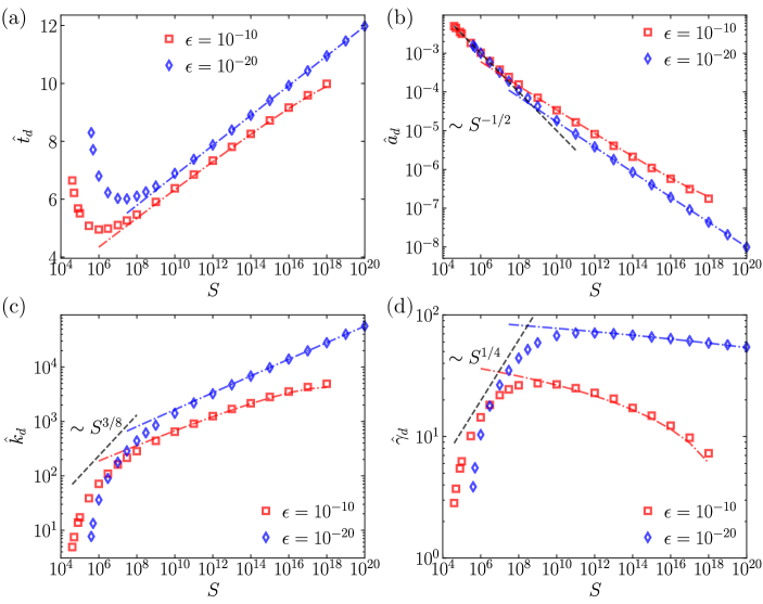
Figure 3: Scalings of $\hat{t}_{d}$, $\hat{a}_{d}$, $\hat{k}_{d}$, and $\hat{\gamma}_{d}$ with respect to the Lundquist number $S$. Here, a constant initial noise spectrum $f_{0}(\hat{k})=\epsilon$ is assumed. The symbols are results obtained by numerical solutions of the model equation, whereas the dash-dotted lines are analytic scaling relations. The black dashed lines are scalings based on the fastest growing mode of a Sweet-Parker current sheet.

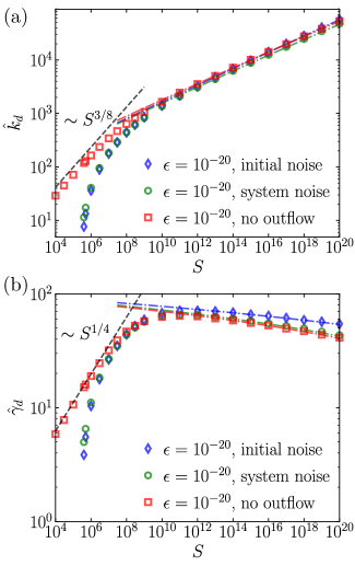
Figure 4: Scalings of $\hat{k}_{d}$ and $\hat{\gamma}_{d}$ with respect to the Lundquist number $S$. Here, a constant noise spectrum $f_{0}(\hat{k})=\epsilon$ is assumed.

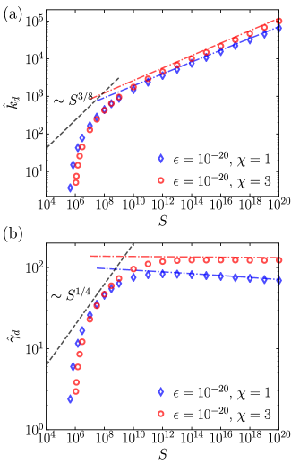
Figure 5: Scalings of $\hat{k}_{d}$ and $\hat{\gamma}_{d}$ with respect to the Lundquist number $S$. Here, a power-law system noise $f_{0}(\hat{k})=\epsilon\hat{k}^{-\chi}$ is assumed.

We have employed several approximations when deriving the analytic scaling relations. These approximations include: (i) ignoring the asymptotic current sheet width $a_{\infty}$ in Eq. (5); (ii) using an approximate linear growth rate Eq. (15) that ignores the $\hat{k}\hat{a}=1$ stability threshold; (iii) ignoring the contribution from the lower bound $\varphi_{0}$ of the integral in Eq. (22); (iv) assuming the initial or system noise spectrum $f_{0}(\hat{k})$ to be slowly varying compared to the exponential factor in Eq. (34); and (v) replacing the integral in (43) by a Gaussian integral and pushing the bounds to $\pm\infty$. Among these approximations, (iv) is an assumption that must be satisfied by the noise spectrum $f(\hat{k}_{0})$; the other approximations can be justified a posteriori in the limit of high-$S$ and low-noise.

We now test the analytic scaling relations with the results from numerical solutions of the model equation. For the numerical solutions, we do not employ any approximation except the linear growth rate, where Eq. (14) with $\zeta=3/2$ is used. Using the approximate linear growth rate is not a significant compromise because the expression is nearly exact; note that the analytic calculation employs a further simplified expression for the linear growth rate, Eq. (15).

To fix ideas, we employ the same setup as in Ref. [Huang et al., 2017], i.e., with $\hat{a}_{0}=1/\pi$ and $\hat{\tau}=\log 2$. We vary the parameters $\epsilon$, $\chi$, and $S$ for cases with either an initial noise or a system noise, with or without the outflow. We integrate the normalized model equation (6) forward in time along characteristics. Because the wavenumber $\hat{k}$ decreases exponentially in time along a characteristic, it is convenient to set the mesh in the wavenumber $\hat{k}$ equispaced with respect $\log\hat{k}$ and set the time step $\Delta\hat{t}=\Delta\log\hat{k}$. In this way, the wavenumber $\hat{k}$ shifts exactly one grid space in one time step, which significantly simplifies the time integration along characteristics. We perform the time integration with a second-order trapezoidal scheme. For cases with system noise, in each time step the solution $f(\hat{k})$ is compared with $f_{0}(\hat{k})$; we set $f(\hat{k})$ to $f_{0}(\hat{k})$ for those $\hat{k}$ where $f(\hat{k})<f_{0}(\hat{k})$. In each time step, we identify the dominant wavenumber and calculate the plasmoid size $\hat{w}$ with Eq. (3), where $\xi=1.5$ has been used. The time integration continues until the disruption condition $\hat{\delta}=\hat{w}$ is met. Then we record $\hat{a}_{d}$, $\hat{k}_{d}$, and $\hat{\gamma}_{d}$ at the disruption time $\hat{t}_{d}$.

The analytic scaling relations involve constants $c_{a}$, $c_{k}$, $c_{\gamma}$, and $c_{\chi}$. These constants depend on $\hat{\tau}$ because they depend on $\varphi_{d}$ that maximizes the function $g(\varphi;\hat{\tau})$; additionally, $c_{a}$ and $c_{\chi}$ also depend on $g(\varphi_{d})$ and $g^{\prime\prime}(\varphi_{d})$. For $\hat{\tau}=\log 2$, we numerically obtain $\varphi_{d}\approx 0.655$, $g(\varphi_{d})\approx 0.841$, and $g^{\prime\prime}(\varphi_{d})\approx-0.820$. If the outflow is neglected, i.e., taking the limit $\hat{\tau}\to 0$, they become $\varphi_{d}\approx 0.784$, $g(\varphi_{d})\approx 0.791$, and $g^{\prime\prime}(\varphi_{d})\approx-0.629$. These values are used in Eqs. (37), (38), (46), and (48) to obtain the constants $c_{a}$, $c_{k}$, $c_{\gamma}$, and $c_{\chi}$. The values of these constants for different settings reported in this work are listed in Table 1. In the following comparisons, we use the precise analytic scaling relations involving the Lambert function, but the leading order approximate scaling relations are almost as good.

We start with a setup having the initial noise $f_{0}(\hat{k})=\epsilon$. The scalings for $\hat{t}_{d}$, $\hat{a}_{d}$, $\hat{k}_{d}$, and $\hat{\gamma}_{d}$ with respect to $S$ are shown in Fig. 3 for two cases $\epsilon=10^{-10}$ and $\epsilon=10^{-20}$. Here, the symbols denote the scalings obtained from numerical solutions, the dash-dotted lines are the analytic scalings, and the black dashed lines are scalings based on the fastest growing mode of the Sweet-Parker current sheet [i.e., by setting $\hat{a}=\hat{a}_{SP}=S^{-1/2}$ in Eqs. (16) and (17)]. We can see that the analytic scalings accurately agree with the numerically results in the high-$S$ regime. On the other hand, while the Sweet-Parker scaling $\hat{a}_{SP}=S^{-1/2}$ agrees with $\hat{a}_{d}$ in the low to moderately-high $S$ regimes, the Sweet-Parker-based scalings for $\hat{k}_{\text{max}}$ and $\hat{\gamma}_{\text{max}}$ considerably depart from the numerical results of $\hat{k}_{d}$ and $\hat{\gamma}_{d}$; the difference is especially substantial when $S$ is low. The discrepancies are due to the stretching effect of outflow that makes the wavelength of the dominant mode significantly longer than that of the fastest growing mode.

Next, we test the analytic scalings for the other two cases: (1) system noise instead of initial noise and (2) ignoring the effects of outflow. Here, we set $f_{0}(\hat{k})=\epsilon$ with $\epsilon=10^{-20}$. We only present the results for $\hat{k}_{d}$ and $\hat{\gamma}_{d}$ since they provide more stringent tests than $\hat{t}_{d}$ and $\hat{a}_{d}$. The scalings of $\hat{k}_{d}$ and $\hat{\gamma}_{d}$ with respect to $S$ are shown in Fig. 4; for comparison, we also show results that have been presented in Fig. 3 for cases of initial noise. We again see that the analytic scalings are in excellent agreement with the numerical results in the high-$S$ regime. In that regime, the scalings of $\hat{k}_{d}$ are quite similar for all three cases; on the other hand, ignoring the effect of the outflow only slightly affects the scaling of $\hat{\gamma}_{s}$ compared to the case with a system noise, whereas $\hat{\gamma}_{s}$ is higher for the case with an initial noise. The linear growth rate $\hat{\gamma}_{s}$ is higher for the initial noise case because the noise decays during the early period when all the modes are stable; therefore, the disruption occurs at a later time compared to the other two cases. As the current sheet is thinner at a later time, the linear growth rate is higher. Note that the Sweet-Parker-based scalings agree quite well with numerical results at the low-$S$ regime when the outflow is ignored, confirming our earlier statement that the discrepancies are due to the effect of the outflow.

The analytic scaling relations are derived under the assumption that the noise spectrum $f_{0}(\hat{k})$ is slowly varying compared to the exponential factor in Eq. (34). For the cases we have tested so far, this assumption is trivially satisfied with $f_{0}(\hat{k})=\epsilon$. Now we test the analytic scalings for a power-law system noise $f_{0}(\hat{k})=\epsilon\hat{k}^{-\chi}$, with $\epsilon=10^{-20}$. Figure 5 shows the scalings of $\hat{k}_{d}$ and $\hat{\gamma}_{d}$ for the cases $\chi=1$ and $\chi=3$. We can see that even for a relatively steep noise spectrum with $\chi=3$, the analytical scalings remain quite accurate.

VI Conclusion

In conclusion, we have derived analytic scaling relations for the phenomenological model of plasmoid-mediated disruption of evolving current sheets, including the effects of the reconnection outflow. The analytic scaling relations are derived for two scenarios, one with an initial noise and another with a system noise. The former is useful for comparison with numerical simulations or laboratory experiments where an initial perturbation can be injected; the latter is more suitable for describing the plasmoid instability in natural systems. If the effects of outflow are neglected, and with a proper translation of notations, the scalings obtained from the present model agree with that from previous works based on a principle of least time,(Comisso et al., 2016, 2017) up to the leading order approximation.

The phenomenological model is valid in the linear regime of the plasmoid instability, up to the point of current sheet disruption. The time scale $t_{d}$ for current sheet disruption is typically on the order of a few Alfvén time $\tau_{A}$. Here, we estimate the Alfvén times for various systems of interest. For a large-scale coronal mass ejection (CME), the post-CME current sheet can extend to a length beyond several times of the solar radius $R_{\odot}\simeq 7\times 10^{8}\text{m}$; the Alfvén speed can be estimated from the speeds of moving blobs in the current sheet, typically in the range of $2\times 10^{5}$ – $10^{6}\text{m/s}$.(Guo et al., 2013; Lin et al., 2015) Assuming $L\sim 10^{9}\text{m}$ and $V_{A}\sim 10^{6}\text{m/sec}$, the Alfvén time $\tau_{A}$ is on the order of $1000$ seconds. For ultraviolet bursts in the solar transition region,(Innes et al., 2015; Chitta et al., 2017) we estimate the current sheet length $L\sim 10^{6}\text{m}$ from forward modeling (Peter et al., 2019) and the Alfvén speed $V_{A}\sim 10^{5}\text{m/sec}$ from the Doppler broadening of emission line profiles, yielding $\tau_{A}\sim 10$ seconds. For laboratory magnetic reconnection experiments,(Jara-Almonte et al., 2016; Olson et al., 2016) the Alfvén time $\tau_{A}$ is typically on the order of microseconds, which is within the temporal resolution of in situ measurements. Thus, it may be possible to test some of the predictions from the phenomenological model with future generations of laboratory experiments.(Ji et al., 2018)

Although the present study focuses on resistive MHD, the methodology is quite general. The analysis could be generalized to include other effects such as viscosity, the Hall effect, or ambipolar diffusion from partially ionized plasmas. It is also important to further test the predictions of the phenomenological model with full resistive MHD simulations, especially in the high-$S$ regime. While the present analytic calculation is limited to the special class of evolving current sheets where the upstream magnetic field remains constant, the phenomenological model could also describe cases where the upstream magnetic field evolves in time, e.g., as in Refs. [Shay et al., 2004] and [Cassak and Drake, 2009]. These directions will be pursued in the future.