Full Convergence of the Iterative Bayesian Update and Applications to Mechanisms for Privacy Protection

Abstract

The iterative Bayesian update (IBU) and the matrix inversion (INV) are the main methods to retrieve the original distribution from noisy data resulting from the application of privacy protection mechanisms. We show that the theoretical foundations of the IBU established in the literature are flawed, as they rely on an assumption that in general is not satisfied in typical real datasets. We then fix the theory of the IBU, by providing a general convergence result for the underlying Expectation-Maximization method. Our framework does not rely on the above assumption, and also covers a more general local privacy model. Finally we evaluate the precision of the IBU on data sanitized with the Geometric, $k$-RR, and Rappor mechanisms, and we show that it outperforms INV in the first case, while it is comparable to INV in the other two cases.

I Introduction

The problem of developing methods for privacy protection while preserving utility has stimulated an active area of research, and several approaches have been proposed. Depending on their architecture, these methods can be distinguished in central and local [1]. The central model assumes the presence of a trusted administrator, who has access to the users’ original data and takes care of the data sanitization. In the local model the users sanitize their data by themselves before they are collected, typically by applying some obfuscation mechanism.

The local model is clearly more robust: it requires no trusted party, and it is less vulnerable to security breaches. Indeed, even if a malicious entity manages to break into the repository, it will only access sanitized data. On the other hand, guaranteeing a good utility in the local model is more challenging than in the central one.

Concerning utility, we ought to distinguish two main categories: the quality of service, and the statistical value of the collected data. The former refers to what the user expects from the service provider, assuming that he has provided voluntarily his data in exchange of some kind of personalized service. The statistical utility, on the other hand, measures the precision of analyses on the obfuscated data w.r.t. those on the original data.

In this paper, we focus on statistical utility and on the local privacy model based on injection of controlled random noise. We assume a collection of noisy data produced by a population of users, and we consider the reconstruction of the original distribution, i.e., the distribution determined by the original data. In the privacy literature the main methods that have been proposed for this purpose are the matrix inversion technique (INV) [2, 3] and the iterative Bayesian update (IBU) [4], [2]. INV has the advantage of being based on simple linear-algebra techniques and some post-processing to obtain a distribution. The post-processing can be a normalization or a projection on the simplex, and we will call the corresponding methods INV-N and INV-P respectively. The IBU is an iterative algorithm that is based on the Expectation-Maximization method well known in statistics, and has the advantage of producing the maximum likelihood estimator (MLE) of the noisy data.

The IBU has recently attracted renewed interest from the community. For example, it has been used in [5, 6, 7, 8, 9], relying on the foundations established in the seminal paper [4]. We have found out, however, that there are various mistakes in the theoretical results of [4]. The general problem is that [4] builds on the convergence result of Wu [10] without paying attention to the assumption that the update process converges to a point in the “interior” of the parameter space (cfr. [10, Section 2.1]). The parameter space, in the case of the IBU, consists of the distributions candidate to be the MLE, i.e., a subset of the $n$-dimensional simplex. The “interior point” assumption excludes, therefore, the cases in which the MLE is in the border of the simplex, i.e., the non-fully-supported distributions. Now, this assumption is not necessarily satisfied in the local privacy model, for at least two reasons. The first is that the original distribution itself (which has high likelihood to be the MLE) may be not fully supported. For example, the Gowalla dataset in San Francisco has “holes”, i.e., cells with no checkins, even on a relatively coarsely discretized map, cfr. Fig. 1 (data available at https://gitlab.com/locpriv/ibu/blob/master/gdata/nsf.txt). This means that the corresponding distribution assigns probability $0$ to those cells. The second reason is that, even if the original distribution is fully supported, the MLE may not be. This can happen because some components of the distribution may be underestimated if they not contribute much to the likelihood of the observed (noisy) data.

The convergence of the IBU to an MLE in [4] (cfr. Theorem 4.3) relies on the MLE being a stationary point, i.e., a point in which the derivatives have value $0$. Indeed, the stationary property would be a consequence of the “interior point” assumption, as proved by Wu [10]. But as shown above, that assumption does not hold, and the MLE is not necessarily a stationary point. We show a counterexample in Section III-C.

In this paper we fix the foundations of the IBU, and we prove the general convergence of the IBU to an MLE, even in the case in which the “interior point” assumption is not satisfied. Furthermore, we prove this result in a more general setting than [4]. Namely, we assume that each user can apply a different mechanism (also with a possibly different level of privacy), and even change the mechanism several times while the data are being collected. In other words, we assume a fully local privacy model. We argue that this is an advantage of our framework, since different users may have different privacy requirements, and even for the same user the requirements may change over time, or depending on the secret to protect.

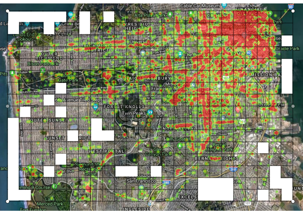
Figure 1: Heatmap of the Gowalla checkins in an area in San Francisco. The white polygons represent sets of cells where there are no checkins.

Another problem in [4] is the claim that the log-likelihood function has a unique global maximum (cfr. Proposition 4.1), from which [4] derives that the MLE is unique (cfr. Theorem 4.4). This is not true in general as we show in Section III-A. As a consequence, Observation 4.1. in [4], stating that as the number of observed data grows the IBU approximates better and better the original distribution, does not hold either; we show a counterexample in Section III-B. Since the whole point of the IBU is to reconstruct as faithfully as possible the original distribution, it is crucial to ensure that the approximation can be done at an arbitrary level of precision. As the above counterexample shows, we get this guarantee only if the MLE is unique. This motivates us to study the conditions of uniqueness (cfr. Section VIII).

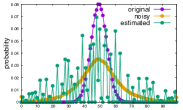
(a) Using INV-N

(b) Using INV-N

(c) Using INV-P

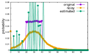
(d) Using INV-P

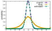
(e) Using EM

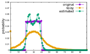
(f) Using EM

Figure 2: Estimating the original distributions from noisy data produced by a geometric mechanism with $\epsilon=0.1$. On the left side, the original data are obtained by sampling a binomial. On the right side, they are sampled from a distribution which is uniform on $\{20,\dots,39\}$ and zero outside this range.

Finally, we compare the performance of the IBU with those of INV-N and INV-P. A similar comparison was done in [2] (resulting in a favorable verdict for the IBU), but the mechanisms used there were rather different from the modern ones. We are interested in comparing their precision on state-of-the-art mechanisms, in particularly the ones used for local differential privacy (LDP) [11, 12] and for differential privacy on metrics ($d_{X}$-DP)[13], whose instantiation to geographical distance is known in the area of location privacy under the name of geo-indistinguishability [14]. Two well-known mechanisms for LDP are Rappor [15] and $k$-randomized-responses ($k$-RR) [12]. As for $d_{X}$-DP and geo-indistinguishability, the typical mechanisms are the Geometric and the Laplace noise. We have experimentally verified that (a) the IBU and INV are more or less equivalent for $k$-RR and Rappor, while (b) there is a striking difference when we use the geo-indistinguiable mechanisms. Figure 2 reports our experiments with two different probability distributions on the original data (a binomial distribution and a distribution uniform on a sub-interval), and applying geometric noise. As we can see, the IBU outperforms by far the INV methods. The experiments are described in detail in Section IX-A.

I-A Contributions

The contributions of this paper are as follows:

• We show that there are various mistakes in the theory of the IBU as it appears in the literature.

• We fix the foundations of the IBU by providing a general convergence theorem.

• The above theorem is actually valid for a generalization of the local privacy model, in which different users can use different mechanisms, and the same input can generate several outputs, possibly under different mechanisms.

• We identify the conditions under which the MLE is unique. This is important, because only if the MLE is unique then we can approximate the original distribution at an arbitrary level of precision.

• We compare IBU and INV on various distributions and mechanisms, showing that IBU outperforms INV in some cases, and is equivalent in the others.

I-B Structure of the paper

Section II presents some preliminaries. Section III describes the mistakes in the foundations of the IBU. In Section IV we establish a general convergence result of EM algorithms. In Section V we generalize the local privacy model, extend the IBU to work on this model, and also prove the convergence of the derived algorithm to the MLEs. In Sections VI, VII we discuss special cases of this algorithm. In Section VIII we study cases in which the MLE is unique. In Section IX we experiment the precision of the IBU compared to INV. Section X describes related work. Finally in Section XI we conclude and describe future work.

The proofs of the various results are available in the appendix. The software used for the experiments is available at gitlab.com/locpriv/ibu.

II Preliminaries

II-A Maximum-likelihood estimators

A statistical model is often used to explain the observed output of a system. Let $\mathcal{O}$ be the set of potential observables, with generic element $o$, and let $O$ be the random variable ranging on $\mathcal{O}$ representing the output. Assume that the probability distribution of $O$ depends on a (possibly multi-dimensional) parameter $\boldsymbol{\theta}$ taking values in a space $\mathcal{C}$. Given an output $o$, the aim is to find the $\boldsymbol{\theta}$ that maximizes the probability of getting $o$, and that therefore is the best explanation of what we have observed. To this purpose, it is convenient to introduce the notion of the log-likelihood function $L:\mathcal{C}\to\mathbb{R}$, defined as

$$L(\boldsymbol{\theta})=\log P(O=o|\boldsymbol{\theta}).$$ (1)

where $P(O=o|\boldsymbol{\theta})$ is the conditional probability of $o$ given $\boldsymbol{\theta}$. The Maximum-Likelihood estimator (MLE) of the unknown parameter is then defined as the $\boldsymbol{\theta}$ that maximizes $L(.)$ (and therefore $P(O=o|\boldsymbol{\theta})$, since $\log$ is monotone). In some cases these maximizers can be computed by analytical techniques, but often, e.g. when the observables are not dependent directly on the parameter, more sophisticated methods are needed.

II-B The Expectation-Maximization framework

The Expectation-Maximization (EM) framework [16, 10, 17] is a powerful method for computing the MLE in various statistical scenarios. This method is used when the statistical model has hidden data that, if known, would make the estimation procedure easier. More precisely, let the hidden data be modeled by a random variable $S$ ranging on $\mathcal{S}$. Then if $S$ is known to have the value $s$, it may be easier to work on the “complete data” log-likelihood $\log P(S=s,O=o|\boldsymbol{\theta})$ rather than on the (incomplete data) log-likelihood in (1). Since the value of $S$ is actually unknown, instead of $\log P(S=s,O=o|\boldsymbol{\theta})$ we consider its expected value, computed using a prior approximation $\boldsymbol{\theta}^{\prime}$ of the parameter. This expectation yields the function $Q(\boldsymbol{\theta}|\boldsymbol{\theta}^{\prime})$ defined as

$$Q(\boldsymbol{\theta}|\boldsymbol{\theta}^{\prime}) =\sum_{s\in\mathcal{S}}P(S=s|O=o;\boldsymbol{\theta}^{\prime})$$

$$\qquad\qquad\qquad\log P(S=s,O=o|\boldsymbol{\theta}).$$ (2)

Let $H(\boldsymbol{\theta}|\boldsymbol{\theta}^{\prime})$ be defined as

$$H(\boldsymbol{\theta}|\boldsymbol{\theta}^{\prime}) =-\sum_{s\in\mathcal{S}}P(S=s|O=o;\boldsymbol{\theta}^{\prime})$$

$$\qquad\qquad\qquad\log P(S=s|O=o;\boldsymbol{\theta}).$$ (3)

It is easy to verify that

$$L(\boldsymbol{\theta})=Q(\boldsymbol{\theta}|\boldsymbol{\theta}^{\prime})+H(\boldsymbol{\theta}|\boldsymbol{\theta}^{\prime}),$$ (4)

Using (4) together with the fact that $H(\boldsymbol{\theta}|\boldsymbol{\theta}^{\prime})\geq H(\boldsymbol{\theta}^{\prime}|\boldsymbol{\theta}^{\prime})$ (by applying Gibb’s inequality) we get the following fundamental property of any EM algorithm:

$$L(\boldsymbol{\theta})-L(\boldsymbol{\theta}^{\prime})\geq Q(\boldsymbol{\theta}|\boldsymbol{\theta}^{\prime})-Q(\boldsymbol{\theta}^{\prime}|\boldsymbol{\theta}^{\prime})\quad\forall\boldsymbol{\theta},\boldsymbol{\theta}^{\prime}\in\mathcal{C}.$$ (5)

The above inequality means that if $\boldsymbol{\theta}$ is chosen to improve $Q(\boldsymbol{\theta}|\boldsymbol{\theta}^{\prime})$ w.r.t. $Q(\boldsymbol{\theta}^{\prime}|\boldsymbol{\theta}^{\prime})$, then $L(\boldsymbol{\theta})$ is also improved w.r.t. $L(\boldsymbol{\theta}^{\prime})$ by at least the same amount. Therefore, $L(\boldsymbol{\theta})$ monotonically grows by iterating between two steps: the expectation in which $Q(\boldsymbol{\theta}|\boldsymbol{\theta}^{\prime})$ is evaluated, and the maximization which computes a $\boldsymbol{\theta}$ that maximizes $Q(\boldsymbol{\theta}|\boldsymbol{\theta}^{\prime})$. Note that, since $L(.)$ is bounded from above by $0$, by the monotone convergence theorem it must converge. Table I summarizes the above notations and other ones used in Sections III and IV.

TABLE I: Notations used in Sections II–IV

$\mathcal{C}$	the parameter space
$\boldsymbol{\theta},\boldsymbol{\theta}^{\prime},\boldsymbol{\theta}^{t}$	elements of $\mathcal{C}$. $\boldsymbol{\theta}^{t}$ is the parameter estimate at time $t$.
$\mathcal{S}$	the space of hidden data.
$S$	random var. representing the hidden data, ranging on $\mathcal{S}$.
$\mathcal{O},\mathcal{Z}$	spaces of observed data.
$O,Z$	random vars representing observed data, ranging on $\mathcal{O},\mathcal{Z}$ respectively.
$o,z$	elements of $\mathcal{O},\mathcal{Z}$ denoting the observed data.
$\mathcal{X}$	the space of input data
$X,X^{i}$	random vars representing the input data, ranging on $\mathcal{X}$.
$\theta_{x}$	probability of $x\in\mathcal{X}$ based on distribution $\boldsymbol{\theta}$.
$A:\mathcal{X}\to\mathcal{Z}$	obfuscation mechanism.
$a_{xz}$	probability that $A$ yields $z$ from $x$.
$\boldsymbol{q}$	empirical distribution on $\mathcal{Z}$.
$q_{z}$	probability of $z\in\mathcal{Z}$ according to $\boldsymbol{q}$.
$L(\boldsymbol{\theta})$	the log-likelihood of $\boldsymbol{\theta}$ w.r.t. the observed data.
$Q(\boldsymbol{\theta}|\boldsymbol{\theta}^{\prime})$	expected complete-data log-likelihood of $\boldsymbol{\theta}$.
$H(\boldsymbol{\theta}|\boldsymbol{\theta}^{\prime})$	difference between $L(\boldsymbol{\theta})$ and $Q(\boldsymbol{\theta}|\boldsymbol{\theta}^{\prime})$ (cfr. (4)).
$M_{\textit{em}}(\boldsymbol{\theta})$	the point-to-set map of the EM algorithm, mapping $\boldsymbol{\theta}$ to a subset of $\mathcal{C}$.
$I$	A proper interval in $\mathbb{R}$.
$\boldsymbol{\alpha}:I\!\to\mathcal{C}$	differentiable curve from $I$ to $\mathcal{C}$.
$\Gamma$	the solution set of an EM algorithm, $\Gamma\subset\mathcal{C}$.

II-C Iterative Bayesian Update procedure

The iterative Bayesian update (IBU) [4] is an instance of the EM method. Consider a set of input data represented by the i.i.d. (independent and identically distributed) random variables $X^{1},X^{2},\dots,X^{n}$, ranging on a space $\mathcal{X}$ and with distribution $\boldsymbol{\theta}$ on $\mathcal{X}$. Let $\theta_{x}$ be the probability of $x\in\mathcal{X}$. Suppose that the value of every $X^{i}$ is independently obfuscated by a given mechanism $A:\mathcal{X}\to\mathcal{Z}$ to yield a noisy observable $z^{i}\in\mathcal{Z}$ as shown in Fig. 3. Given the observations $z^{i}$ for $i=1,2,\dots,n$, the IBU approximates a MLE for them as follows. Let $\boldsymbol{q}=(q_{z}:z\in\mathcal{Z})$ be the empirical distribution on $\mathcal{Z}$, where $q_{z}$ is the number of times $z$ is observed divided by $n$. Let $a_{xz}$ be the probability that $A$ yields $z$ from $x$. The IBU starts with a full-support distribution $\boldsymbol{\theta}^{0}$ on $\mathcal{X}$ (e.g., the uniform distribution), and iteratively produces new distributions by the update rule

$$\theta^{t+1}_{x} = \sum_{z\in\mathcal{Z}}q_{z}\,\frac{\theta^{t}_{x}a_{xz}}{\sum_{u\in\mathcal{X}}\theta^{t}_{u}a_{uz}}\quad\forall x\in\mathcal{X}.$$ (6)

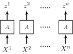
Figure 3: The obfuscation model on which IBU is defined. User inputs are $X^{1},X^{2},\dots,X^{n}$ taking values in $\mathcal{X}$. Obfuscating them, by the mechanism $A$, yields the noisy data $z^{1},z^{2},\dots,z^{n}\in\mathcal{Z}$.

The convergence of this algorithm has been studied in [4], concluding that the IBU converges to a unique MLE which is stationary in the space of distributions. In the following section we revisit these claims and we prove, by counterexamples, that they do not always hold.

III Revisiting the properties of IBU and MLEs

III-A The MLE may not be unique

Let $\mathcal{X}=\{1,2,3\}$, and consider the obfuscation mechanism $A:\mathcal{X}\to\mathcal{X}$ represented by the following stochastic matrix (where the inputs are on the rows and the outputs are on the columns. For instance, $a_{11}=\nicefrac{{1}}{{2}}$, $a_{12}=\nicefrac{{1}}{{3}}$, etc.).

$$A = \begin{bmatrix}\nicefrac{{1}}{{2}}&\nicefrac{{1}}{{3}}&\nicefrac{{1}}{{6}}\\ \nicefrac{{1}}{{3}}&\nicefrac{{1}}{{3}}&\nicefrac{{1}}{{3}}\\ \nicefrac{{1}}{{6}}&\nicefrac{{1}}{{3}}&\nicefrac{{1}}{{2}}\end{bmatrix}.$$ (7)

Assume that three users apply this mechanism and we observe $Z^{1}=1,Z^{2}=2,Z^{3}=3$. Given a generic distribution $\boldsymbol{\theta}=(\theta_{1},\theta_{2},\theta_{3})$ on $\mathcal{X}$, the log-likelihood is $L(\boldsymbol{\theta})=\log P(Z^{1}=1,Z^{2}=2,Z^{3}=3\mid\boldsymbol{\theta})=\log P(Z^{1}=1\mid\boldsymbol{\theta})+\log P(Z^{2}=2\mid\boldsymbol{\theta})+\log P(Z^{3}=3\mid\boldsymbol{\theta})=\log(\nicefrac{{\theta_{1}}}{{2}}+\nicefrac{{\theta_{2}}}{{3}}+\nicefrac{{\theta_{3}}}{{6}})+\log(\nicefrac{{1}}{{3}})+\log(\nicefrac{{\theta_{1}}}{{6}}+\nicefrac{{\theta_{2}}}{{3}}+\nicefrac{{\theta_{3}}}{{2}})$. Fig. 4 shows the plot of $L(\boldsymbol{\theta})$, where we consider only the components $\theta_{1},\theta_{3}$ of $\boldsymbol{\theta}$: $\theta_{2}$ is redundant since $\theta_{2}=1-\theta_{1}-\theta_{3}$. As we can see, there are infinitely many MLEs, because every $\boldsymbol{\theta}$ with $\theta_{1}=\theta_{3}$ is a maximum of $L(\boldsymbol{\theta})$, including for instance $(0,1,0)$ and $(\nicefrac{{1}}{{2}},0,\nicefrac{{1}}{{2}})$. This contradicts Proposition 4.1 and Theorem 4.4 of [4] and also a similar claim in [5] (Section 3.2) that was based on the above results. The implications of this counterexample lead to another refutation as shown in the following.

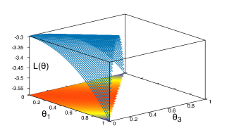
Figure 4: The log-likelihood function $L(\boldsymbol{\theta})$ for the distributions on $\mathcal{X}=\{1,2,3\}$ given the mechanism $A$ and the observables $\{1,2,3\}$.

III-B The IBU may not approximate the true distribution

Given a mechanism $A$ and a distribution $\boldsymbol{\theta}$ on $\mathcal{X}$, as the number $n$ of input grows, the empirical distribution $\boldsymbol{q}$ tends probabilistically to the true distribution induced on the output, which is $\boldsymbol{\theta}A$. From this, [4] deduces (Observation 4.1) that the result of the IBU approximates the true distribution $\boldsymbol{\theta}$ as $n\rightarrow\infty$. If $A$ is not invertible, however, there may be two different $\boldsymbol{\theta}$, $\boldsymbol{\theta}^{\prime}$ such that $\boldsymbol{\theta}A=\boldsymbol{\theta}^{\prime}A$, which means that $\boldsymbol{\theta}$ and $\boldsymbol{\theta}^{\prime}$ cannot be statistically distinguished on the basis of the empirical distribution observed in output, no matter how large $n$ is. The implication for the IBU is that, even in the “optimal” case that $\boldsymbol{q}=\boldsymbol{\theta}A$, where $\boldsymbol{\theta}$ is the true distribution, the IBU may converge to a different $\boldsymbol{\theta}^{\prime}$ if $\boldsymbol{\theta}^{\prime}A=\boldsymbol{q}$ (both $\boldsymbol{\theta}$ and $\boldsymbol{\theta}^{\prime}$ are MLE of $\boldsymbol{q}$). This contradicts Observation 4.1 in [4].

As an example, consider again the mechanism $A$ defined in (7) and consider the empirical distribution $\boldsymbol{q}=(\nicefrac{{1}}{{3}},\nicefrac{{1}}{{3}},\nicefrac{{1}}{{3}})$. All distributions in the set $\Theta=\{\boldsymbol{\theta}:\theta_{1}=\theta_{3}\}$ satisfy $\boldsymbol{\theta}A=\boldsymbol{q}$. From this it is easy to see that all distributions in $\Theta$ are fixed points of the transformation (6), i.e., $\boldsymbol{\theta}^{t+1}=\boldsymbol{\theta}^{t}$ for all $\boldsymbol{\theta}^{t}\in\Theta$. This means that the IBU can converge to any $\boldsymbol{\theta}^{\prime}\in\Theta$ (depending on the starting distribution), instead of the true $\boldsymbol{\theta}$. For instance, $\boldsymbol{\theta}$ could be $(0,1,0)$ and $\boldsymbol{\theta}^{\prime}$ could be $(\nicefrac{{1}}{{2}},0,\nicefrac{{1}}{{2}})$.

III-C The MLE may not be stationary

Theorem 4.3 in [4] relies on MLE being stationary, i.e., that the derivatives of $L(\boldsymbol{\theta})$ have value $0$ on the MLE, and such property is (erroneously) claimed to hold. The following example shows that this is not true in general. Let again $\mathcal{X}=\{1,2,3\}$, and consider a $3$-RR obfuscation mechanism $A^{\prime}:\mathcal{X}\to\mathcal{X}$ defined by the following matrix.

$$A^{\prime} = \begin{bmatrix}\nicefrac{{1}}{{2}}&\nicefrac{{1}}{{4}}&\nicefrac{{1}}{{4}}\\ \nicefrac{{1}}{{4}}&\nicefrac{{1}}{{2}}&\nicefrac{{1}}{{4}}\\ \nicefrac{{1}}{{4}}&\nicefrac{{1}}{{4}}&\nicefrac{{1}}{{2}}\end{bmatrix}.$$ (8)

Assume that four users apply this mechanism and we get the observables $Z^{1}=1,Z^{2}=2,Z^{3}=2$ and $Z^{4}=3$. The log-likelihood is $L(\boldsymbol{\theta})=\log(\nicefrac{{\theta_{1}}}{{2}}+\nicefrac{{\theta_{2}}}{{4}}+\nicefrac{{\theta_{3}}}{{4}})+2\log(\nicefrac{{\theta_{1}}}{{4}}+\nicefrac{{\theta_{2}}}{{2}}+\nicefrac{{\theta_{3}}}{{4}})+\log(\nicefrac{{\theta_{1}}}{{4}}+\nicefrac{{\theta_{2}}}{{4}}+\nicefrac{{\theta_{3}}}{{2}})$. The plot of $L(\boldsymbol{\theta})$ (Fig. 5) shows that the unique MLE is $(0,1,0)$. On $(0,1,0)$ the partial derivatives are $\partial L(\boldsymbol{\theta})/\partial\theta_{1}=\partial L(\boldsymbol{\theta})/\partial\theta_{3}=-0.5$, hence $(0,1,0)$ is not stationary. We also note that the likelihood surface has no stationary points at all.

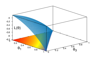
Figure 5: The log-likelihood function $L(\boldsymbol{\theta})$ for the distributions on $\mathcal{X}=\{1,2,3\}$ given the mechanism matrix $A^{\prime}$ and observables $\{1,2,2,3\}$.

III-D The IBU may not converge to an interior distribution

The above misconception in [4] follows from using the EM properties derived in [10] while ignoring an assumption underlying these properties. That is the limit of the EM updates is interior in the parameter space (the probability simplex in our case) (See Section 2.1 in [10]). The problem is that this assumption may be violated when the IBU is applied to the outcomes of an obfuscation mechanism. For example, applying IBU to $A^{\prime}$ defined in (8) and the observations $\{1,2,2,3\}$ yields the distribution $(0,1,0)$ which is clearly not interior. Note from Fig. 5 that this distribution is the required MLE which we prove later in this paper (Theorem V-D).

IV Full convergence of EM algorithms

In this section we establish a convergence result of the EM algorithms that does not rely on the hypothesis that the limit points of the generated sequence $(\boldsymbol{\theta}^{t})_{t\in\mathbb{N}}$ are interior in $\mathcal{C}$. This effort is motivated by the fact that, as discussed in the introduction, such hypothesis is usually not satisfied by typical datasets, e.g. Gowalla, in the contexts of quantitative information flow and privacy.

In the following we will assume, like [16, 10], that the parameter space $\mathcal{C}$ is a subset of the $m$-dimensional Euclidean space. However we abstract from the assumption made in these papers that the limit points are interior to $\mathcal{C}$, and describe an extended solution set $\Gamma$ to which the EM algorithm converges. We start by defining a curve in $\mathcal{C}$ as a differentiable function $\boldsymbol{\alpha}:I\to\mathcal{C}$, where $I$ is a proper (i.e. non singleton) interval in $\mathbb{R}$. Then we can define stationary and local maxima for the log-likelihood function along a curve as follows

Definition 1 (Stationary point along a curve).

Consider a parameter space $\mathcal{C}\subset\mathbb{R}^{m}$, and a curve $\boldsymbol{\alpha}:I\to\mathcal{C}$. Let $\boldsymbol{\theta}^{\prime}$ be a point lying on $\boldsymbol{\alpha}$, i.e. $\boldsymbol{\theta}^{\prime}=\boldsymbol{\alpha}(\tau^{\prime})$ for some $\tau^{\prime}\in I$. Then $\boldsymbol{\theta}^{\prime}$ is stationary for the log-likelihood $L(.)$ along $\boldsymbol{\alpha}$ if ${dL(\boldsymbol{\alpha}(\tau))}/{d\tau}=0$ at $\tau^{\prime}$.

Definition 2 (Local maxima along a curve).

Consider a parameter space $\mathcal{C}\subset\mathbb{R}^{m}$, and a curve $\boldsymbol{\alpha}:I\to\mathcal{C}$. Let $\boldsymbol{\theta}^{\prime}$ be a point lying on $\boldsymbol{\alpha}$, i.e. $\boldsymbol{\theta}^{\prime}=\boldsymbol{\alpha}(\tau^{\prime})$ for some $\tau^{\prime}\in I$. Then $\boldsymbol{\theta}^{\prime}$ is a local maximizer for the log-likelihood $L(.)$ along $\boldsymbol{\alpha}$ if there is $\delta>0$ such that for every $\tau\in I$ satisfying $|\tau-\tau^{\prime}|<\delta$ it holds $L(\boldsymbol{\alpha}(\tau))\leq L(\boldsymbol{\alpha}(\tau^{\prime}))$.

Now we can define our extended solution set $\Gamma$.

Definition 3 (Extended solution set).

Consider a parameter space $\mathcal{C}\subset\mathbb{R}^{m}$. Then $\Gamma$ is the set of all points $\boldsymbol{\theta}^{\prime}$ such that for each curve $\boldsymbol{\alpha}$ on which $\boldsymbol{\theta}^{\prime}$ lies, either $\boldsymbol{\theta}^{\prime}$ is stationary or it a local maximum for the log-likelihood $L(.)$ along $\boldsymbol{\alpha}$.

Clearly the extended solution set $\Gamma$ is larger than the traditional set of stationary points, for which the derivatives must be $0$ along every curve. In fact the extended set allows each of its members to be, along each curve, either stationary or a local maximizer (or both).

We show that the limits of any sequence generated by an EM algorithm must lie in $\Gamma$, and the log-likelihood converges to a value corresponding to an element in $\Gamma$.

[EM full convergence]theoremEMconvergence Consider a parameter space $\mathcal{C}\subset\mathbb{R}^{m}$, and an EM algorithm in which $L(.)$ is continuous on $\mathcal{C}$, and $Q(\boldsymbol{\theta}|\boldsymbol{\theta}^{\prime})$ is continuous with respect to $\boldsymbol{\theta}$ and $\boldsymbol{\theta}^{\prime}$. Let $(\boldsymbol{\theta}^{t})_{t\in\mathbb{N}}$ be any generated sequence that is contained in a compact subset of $\mathcal{C}$. Then all the limit points of this sequence are in $\Gamma$ and $L(\boldsymbol{\theta}^{t})$ converges monotonically to $L(\hat{\boldsymbol{\theta}})$ for some $\hat{\boldsymbol{\theta}}\in\Gamma$. We remark that Theorem 3 extends Theorem 2 of [10] which describes the convergence to stationary points based on an assumption that the limit points of the EM sequence are interior in the $\mathcal{C}$. Our theorem is stronger since it confirms the convergence of the algorithm to the likelihood maximizers whether they are stationary in the interior or lying on the border of $\mathcal{C}$. In general there is no guarantee that they are also global maximizers (i.e., MLEs), but if $\mathcal{C}$ is convex and the likelihood function is concave, then they are MLEs. theoremconvex Let $\mathcal{C}$ be a convex parameter space, and $L(.)$ be a concave log-likelihood function over $\mathcal{C}$. Then the extended solution set $\Gamma$ is exactly the set of global maximizers of $L(.)$. The next section introduces our local privacy model LPM and shows that the conditions of Theorem 3 are satisfied for it, so that the EM algorithm yields always a global maximizer.

V Local privacy model

TABLE II: Additional notation used in Sections V – VIII

$Z^{i}=(Z^{i}_{j})$	a multivariate random vector representing the output at index $i$.
$\boldsymbol{z}^{i}=(z^{i}_{j})$	the output vector at index $i$ (i.e. the value of $Z^{i}$), $z^{i}_{j}$ is the $j$-th observable in the vector $\boldsymbol{z}^{i}$.
$k_{i}$	the length of the vector $\boldsymbol{z}^{i}$, i.e. the number of observables at index $i$.
$A^{ij}$	the matrix of the mechanism used to obfuscate input $X^{i}$ to yield the value of $Z^{i}_{j}$.
$\boldsymbol{G}=[g_{xi}]$	the outputs probability matrix, with $g_{xi}$ being the probability of the observed output at index $i$ given that $X^{i}=x$.
$\boldsymbol{G}(\mathcal{I}^{\prime})$	a matrix consisting only the columns of $\boldsymbol{G}$ that correspond to the outputs in $\mathcal{I}^{\prime}$ (Section VIII).

Let $\mathcal{X}$ be the space of sensitive data of the users. We call the datum of every user an input to the system. The inputs are assumed to be independent and drawn from the same probability distribution $\boldsymbol{\theta}=(\theta_{x}:\forall x\in\mathcal{X})$, hence represented by i.i.d. random variables $X^{i}\sim\boldsymbol{\theta}$ where $i=1,2,\dots,n$ and $n$ is the number of inputs. For convenience we will denote the set of indices $\{1,2,\dots,n\}$ by $\mathcal{I}$. We assume that every input $X^{i}$ is obfuscated by $k_{i}$ mechanisms to yield a multivariate random variable $Z^{i}=(Z^{i}_{1},Z^{i}_{2},\dots,Z^{i}_{k_{i}})$, where the elementary variables $Z^{i}_{j}$ may have different domains. We also denote the observed realization of $Z^{i}$ by $\boldsymbol{z}^{i}=(z^{i}_{1},z^{i}_{2},\dots,z^{i}_{k_{i}})$. The mechanisms used to produce the elements of $\boldsymbol{z}^{i}$ may vary in their definition and level of privacy. For example if $\mathcal{X}$ is a set of locations, then an input $i$ may yield the output $\boldsymbol{z}^{i}=(z^{i}_{1},z^{i}_{2})$ by running first a Laplace mechanism that generates the noisy location $z^{i}_{1}$ and then a cloaking mechanism that produces $z^{i}_{2}$. We assume that every obfuscation mechanism used in the process is known. This allows to compute the probability $P(Z^{i}=\boldsymbol{z}^{i}|X^{i}=x)$ for every $x\in\mathcal{X}$.

Definition 4 (Outputs probability matrix).

The outputs probability matrix, $\boldsymbol{G}=[g_{xi}]$, associates to every $x\in\mathcal{X}$, and every $i\in\mathcal{I}$ the conditional probability $g_{xi}$ of yielding the observed output value at $i$ when $x$ is the value of the corresponding input, that is $g_{xi}=P(Z^{i}=\boldsymbol{z}^{i}|X^{i}=x).$

Note that $\boldsymbol{G}$ is not necessarily square since it consists of $|\mathcal{X}|$ rows and $n$ columns. It is not stochastic either, since its individual columns correspond to the indices $\mathcal{I}$ at which the outputs are drawn using possibly different mechanisms, and from possibly different domains. $\boldsymbol{G}$ is constructed as follows: Let $A^{ij}=[a^{ij}_{xz}]$ be the matrix of the mechanism that was applied by user $i$ to report his $j$th observable $z^{i}_{j}$. Then $g_{xi}=\prod_{j=1}^{k_{i}}a^{ij}_{xz^{i}_{j}}.$ Table II summarizes the above notations together with others that will be used later. Fig. 6 illustrates our local privacy model (LPM).

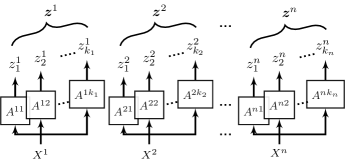
Figure 6: The local privacy model. User inputs are $X^{1},\dots,X^{n}$, and corresponding output vectors are $\boldsymbol{z}^{1},\dots,\boldsymbol{z}^{n}$.

V-A The space of distributions and the likelihood function

In the LPM, we require to find the distribution $\boldsymbol{\theta}$ on $\mathcal{X}$ that maximizes the log-likelihood function $L(.)$. Therefore, we define our space of distributions to include only those having a finite log-likelihood.

$$\mathcal{C}=\{\boldsymbol{\theta}\in\mathbb{R}^{|\mathcal{X}|}:\theta_{x}\geq 0\,\forall x\in\mathcal{X},\sum_{x\in\mathcal{X}}\theta_{x}=1,L(\boldsymbol{\theta})>-\infty\}.$$ (9)

The condition $L(\boldsymbol{\theta})>-\infty$ assures the continuity of $L(.)$ everywhere in $\mathcal{C}$. This is essential for the convergence of the EM algorithm as stated by Theorem 3. The log-likelihood function $L(\boldsymbol{\theta})$ is the logarithm of the joint probability of observed output vectors assuming that every input follows the distribution $\boldsymbol{\theta}$. Since the outputs at $i=1,2,\dots,n$ are independent, $L(\boldsymbol{\theta})$ can be written as $L(\boldsymbol{\theta})=\sum_{i=1}^{n}L_{i}(\boldsymbol{\theta})$, where $L_{i}(\boldsymbol{\theta})=\log\sum_{x\in\mathcal{X}}\theta_{x}\,g_{xi}$ is the likelihood of $\boldsymbol{\theta}$ with respect to the observed output at $i$. Therefore

$$L(\boldsymbol{\theta})=\sum_{i=1}^{n}\log\sum_{x\in\mathcal{X}}\theta_{x}\,g_{xi}.$$ (10)

A distribution $\hat{\boldsymbol{\theta}}$ is a maximum likelihood estimator (MLE) on $\mathcal{X}$ if it maximizes the log-likelihood $L(.)$, i.e.

$$\hat{\boldsymbol{\theta}}\in\operatornamewithlimits{argmax}_{\boldsymbol{\theta}}L(\boldsymbol{\theta}).$$ (11)

In general there may be more than one MLE, depending on the matrix $\boldsymbol{G}$. Therefore the right side of (11) identifies the set of MLEs rather than a single distribution.

V-B Evaluating an MLE using an EM algorithm

In the following we derive an EM instance algorithm that evaluates a likelihood maximizer $\hat{\boldsymbol{\theta}}$ over $\mathcal{X}$. This algorithm starts with an initial distribution $\boldsymbol{\theta}^{0}$ and then iteratively yields a sequence of estimators $(\boldsymbol{\theta}^{t})$, such that the log-likelihood $L(\boldsymbol{\theta}^{t})$ monotonically increases with $t$. We now show how to derive the elements of this sequence. The expected complete-data likelihood $Q(.|.)$ can be written as

$$Q(\boldsymbol{\theta}|\boldsymbol{\theta}^{t})=\mathbf{E}\left[\log P(\land_{i=1}^{n}X^{i},Z^{i}|\boldsymbol{\theta})|\land_{i=1}^{n}Z^{i}=\boldsymbol{z}^{i};\boldsymbol{\theta}^{t}\right].$$

[E-step]theoremestep The value of $Q(\boldsymbol{\theta}|\boldsymbol{\theta}^{t})$ is given by

$$Q(\boldsymbol{\theta}|\boldsymbol{\theta}^{t}) =\sum_{x\in\mathcal{X}}\psi_{x}(\boldsymbol{z},\boldsymbol{\theta}^{t})\log\theta_{x}+K(\boldsymbol{\theta}^{t})$$ (12)

where $\psi_{x}(\boldsymbol{z},\boldsymbol{\theta}^{t})=\sum_{i=1}^{n}P(X^{i}=x|Z^{i}=\boldsymbol{z}^{i};\boldsymbol{\theta}^{t})$ and $K(.)$ is a continuous function depending only on $\boldsymbol{\theta}^{t}$. The authors of [4] studied a special case of our setting, that is when the mechanisms are identical and every output vector $\boldsymbol{z}^{i}$ is singleton. However their expression of $Q$ in [4, Theorem 4.1] is not an instance of ours. This is because they define $Q(\boldsymbol{\theta}|\boldsymbol{\theta}^{t})$ as $\mathbf{E}\left[\log P(\land_{i=1}^{n}X^{i}|\boldsymbol{\theta})|\land_{i=1}^{n}Z^{i}=\boldsymbol{z}^{i};\boldsymbol{\theta}^{t}\right]$, which we believe is not consistent with the standard notion of complete-data log-likelihood presented in Section II-B.

Now the maximization step of the algorithm evaluates the new update $\boldsymbol{\theta}^{t+1}$ to be the maximizer of $Q(.|\boldsymbol{\theta}^{t})$ with fixed $\boldsymbol{\theta}^{t}$. The following theorem characterizes $\boldsymbol{\theta}^{t+1}$. [M-step]theoremmstep Let $\boldsymbol{\theta}^{t+1}$ be the value of $\boldsymbol{\theta}$ that maximizes $Q(\boldsymbol{\theta}|\boldsymbol{\theta}^{t})$ in the M-step. Then $\boldsymbol{\theta}^{t+1}$ is given by

$$\boldsymbol{\theta}^{t+1}_{x}=1/n\sum_{i=1}^{n}P(X^{i}=x|Z^{i}=\boldsymbol{z}^{i};\boldsymbol{\theta}^{t})\quad\forall x\in\mathcal{X}.$$ (13)

In light of the above theorem we note that it is important to start the algorithm with a fully-supported distribution $\boldsymbol{\theta}^{0}$. In fact, if $\theta^{0}_{x}=0$ (13) implies that $\theta_{x}^{t}=0$ for all $t>0$, which means entirely excluding $x$ from the estimation process.

V-C Estimation algorithm

Using the update statement in Theorem V-B, the general EM Algorithm 1 yields an estimator $\hat{\boldsymbol{\theta}}$ for the hidden distribution over $\mathcal{X}$. We show in Section V-D that this estimator is a MLE but may not be unique. The input data of this algorithm are the pairs $(z^{i}_{j},A^{ij})$ for every $i,j$ where $z^{i}_{j}$ is the $j$th observable in the output $\boldsymbol{z}^{i}$, and $A^{ij}$ is the matrix of the mechanism used to yield $z^{i}_{j}$. These data are then used to evaluate the probabilities $g_{xi}$, which are used to obtain $\boldsymbol{\theta}^{t+1}$ based on Theorem V-B.

Data: $\left((z^{i}_{j},A^{ij}=[a^{ij}_{xz}]):i\in\mathcal{I},1\leq j\leq k_{i}\right)$ and $\delta>0$ ;

Result: Approximate the MLE $\hat{\boldsymbol{\theta}}$ in (11).

Compute: $g_{xi}=P(Z^{i}=\boldsymbol{z}^{i}|X_{i}=x)=\prod_{j=1}^{k_{i}}a^{ij}_{xz^{i}_{j}}\quad\forall i,x:i\in\mathcal{I},x\in\mathcal{X}$;

Set $t=0$ and $\boldsymbol{\theta}^{0}$ to any distribution over $\mathcal{X}$ with $\theta^{0}_{x}>0$ for every $x\in\mathcal{X}$;

repeat

       Set $\theta^{t+1}_{x}=(1/n)\sum_{i=1}^{n}\frac{\theta^{t}_{x}g_{xi}}{\sum_{u\in\mathcal{X}}\theta^{t}_{u}g_{ui}}$;

       Set $t=t+1$ ;

      

until  $|L(\boldsymbol{\theta}^{t})-L(\boldsymbol{\theta}^{t-1})|<\delta$ ;

return $\boldsymbol{\theta}^{t}$

Algorithm 1 An EM algorithm for estimating the distribution over the hidden data

The condition $\theta^{0}_{x}>0$ for all $x\in\mathcal{X}$ is important not only to involve all the elements of $\mathcal{X}$ in the estimation process as noted earlier, but also to guarantee that $L(\boldsymbol{\theta}^{0})>-\infty$. The latter condition together with the fact that $L(\boldsymbol{\theta}^{t})$ is increasing with $t$, ensures that the sequence of estimates $\boldsymbol{\theta}^{t}$ generated by the algorithm is contained in a compact subset of $\mathcal{C}$. lemmacompact For any $L^{-}\in\mathbb{R}$ (i.e., $L^{-}>-\infty$), let $\mathcal{C}^{\prime}=\{\boldsymbol{\theta}\in\mathcal{C}:L(\boldsymbol{\theta})\geq L^{-}\}$. Then $\mathcal{C}^{\prime}$ is a compact subset of $\mathcal{C}$. This property meets the conditions in Theorem 3, ensuring the convergence of $\boldsymbol{\theta}^{t}$ to the extended solution set $\Gamma$.

V-D Convergence of the estimation algorithm to a MLE

The objective of every EM algorithm is to yield the MLE for the hidden parameter. In this respect we recall that an EM algorithm in general may yield a stationary point which is not necessarily a global maximizer. However in the application of EM to our LPM, it turns out that Algorithm 1 yields a global maximizer.

lemmaconvexityLPM Let $\mathcal{C}$ and $L(.)$ be defined as in (9) and (10) respectively. Then $\mathcal{C}$ is convex and $L(.)$ is concave on $\mathcal{C}$.

Theorems 3 and 3, whose conditions are ensured by Lemmas 1 and V-D respectively, allow to prove that in our LPM setting the EM algorithm 1 converges to a MLE. [Convergence to MLEs]theoremalgconv Consider any sequence $(\boldsymbol{\theta}^{t})_{t\in\mathbb{N}}$ of distributions generated by Algorithm 1. Then $L(\boldsymbol{\theta}^{t})$ converges monotonically to $L(\hat{\boldsymbol{\theta}})$ where $\hat{\boldsymbol{\theta}}$ is a global maximizer of $L(.)$. It is important to note that $L(.)$ is not strictly concave in general, which means we may have many MLEs as exemplified earlier in Section III-A.

VI Single input

In the following we consider the instance of our LPM when the system has only one input $X$ which is obfuscated multiple times to yield a vector of observables $\boldsymbol{z}$. We will consider both the cases when various mechanisms are used to produce the elements of $\boldsymbol{z}$, and when only one is used.

VI-A Obfuscation by various mechanisms

Suppose that the input $X$ is obfuscated by $k$ arbitrary mechanisms to produce the observed output $\boldsymbol{z}=(z_{1},z_{2},\dots,z_{k})$, as shown in Fig. 7.

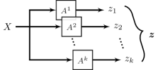
Figure 7: The local privacy model for a single input. The user hidden input is $X$, and corresponding output vector is $\boldsymbol{z}=(z_{1},z_{2},\dots,z_{k})$.

The following theorem characterizes the MLE in this scenario. [MLE for a single input]theoremmlsingleinp Let $X$ be drawn from a hidden distribution over $\mathcal{X}$. Suppose $X$ is obfuscated to produce an output $\boldsymbol{z}=(z_{1},z_{2},\dots,z_{k})$. Then a distribution $\hat{\boldsymbol{\theta}}$ over $\mathcal{X}$ is an MLE if and only if

$$\sum_{x\in\hat{\mathcal{X}}}\hat{\theta}_{x}=1\quad\textit{where}\quad\hat{\mathcal{X}}=\operatornamewithlimits{argmax}_{x\in\mathcal{X}}P(\boldsymbol{z}|x).$$

Theorem 7 states that the MLEs are determined by the subset $\hat{\mathcal{X}}$ consisting of the elements of $\mathcal{X}$ that maximize $P(\boldsymbol{z}|x)$. In particular, every distribution that assigns total probability $1$ to the elements of $\hat{\mathcal{X}}$ is a MLE. It is therefore clear from Theorem 7 that we may have one or infinitely many MLEs depending on $|\hat{\mathcal{X}}|$. In fact if $\hat{\mathcal{X}}=\{x\}$, i.e. it is singleton, then the MLE is unique, namely the one having $P(x)=1$. On the other hand, if $|\hat{\mathcal{X}}|>1$, then there are infinitely many MLEs. This observation is yet another refusal for the claim made in [4, Proposition 4.1] that the log-likelihood function has always a unique MLE.

Finally we recall that every probability $P(\boldsymbol{z}|x)$, which is denoted by $g_{x1}$ (as in Definition 4), is evaluated from the $k$ obfuscation mechanisms (shown in Fig. 7) that produced the elements of $\boldsymbol{z}$ . Let $a^{j}_{xz}$ be the probability of the mechanism $A^{j}$ to yield an observable $z$ from $x$. Then $g_{x1}=\prod_{j=1}^{k}a^{j}_{xz_{j}}.$

VI-B Obfuscation by identical mechanisms

Suppose now that the single input $X$ is obfuscated by a fixed mechanism $A$ to yield the $k$ observables of the output vector $\boldsymbol{z}=(z_{1},z_{2},\dots,z_{k})$. In this case the elements of $\boldsymbol{z}$ belong all to the same set $\mathcal{Z}$, and therefore we can construct an empirical distribution $\boldsymbol{q}=(q_{z}:z\in\mathcal{Z})$ where $q_{z}$ is the proportion of $z$ in the observed vector $\boldsymbol{z}$, i.e. the number of times $z$ appears in $\boldsymbol{z}$ divided by $k$. Let $a_{xz}$ be the conditional probability of the mechanism to yield $z$ when its input is $x$. Then

$$g_{x1} = \prod_{j=1}^{k}a_{xz_{j}}\;=\;\prod_{z\in\mathcal{Z}}(a_{xz})^{kq_{z}}.$$ (14)

From Theorem 7 and (14) we then derive

$$\hat{\mathcal{X}} = \operatornamewithlimits{argmax}_{x\in\mathcal{X}}g_{x1}\;=\;\operatornamewithlimits{argmax}_{x\in\mathcal{X}}\sum_{z\in\mathcal{Z}}q_{z}\log a_{xz}.$$ (15)

The above equation can also be interpreted using the Kullback-Leibler divergence $D_{\textit{KL}}$ [18]. In fact, if we denote by $\boldsymbol{a}_{x}$ the conditional distribution of the mechanism for $x\in\mathcal{X}$, we have $D_{\textit{KL}}(\boldsymbol{q}\,||\,\boldsymbol{a}_{x})=H(\boldsymbol{q})-\sum_{z\in\mathcal{Z}}q_{z}\log a_{xz}$, where $H(\boldsymbol{q})$ is the entropy of $\boldsymbol{q}$, which is a constant because $\boldsymbol{q}$ is fixed. Then, from (15) we get

$$\hat{\mathcal{X}} = \operatornamewithlimits{argmin}_{x\in\mathcal{X}}\,D_{\textit{KL}}(\boldsymbol{q}\,||\,\boldsymbol{a}_{x}).$$ (16)

In other words, the elements $x\in\hat{\mathcal{X}}$ are exactly those for which the mechanism distributions $\boldsymbol{a}_{x}$ are most similar to the observed empirical distribution $\boldsymbol{q}$ (w.r.t. $D_{\textit{KL}}$).

VI-C Relation with the probability of error

We consider now the impact of the length $k$ of the observed vector $\boldsymbol{z}$ on the ML estimation. Suppose that the real input value is $\bar{x}$. Then the observables in the vector $\boldsymbol{z}$ are drawn from $\boldsymbol{a}_{\bar{x}}$. From [18, Chapter 11], we have

$$P\left(D_{\textit{KL}}(\boldsymbol{q}\,||\,\boldsymbol{a}_{\bar{x}})>\delta\right) \leq (1+k)^{|\mathcal{Z}|}\,2^{-k\delta}.$$ (17)

This means that the empirical distribution $\boldsymbol{q}$ converges exponentially (as $k\to\infty$) to $\boldsymbol{a}_{\bar{x}}$. If $\boldsymbol{a}_{\bar{x}}$ is different from all other rows of the mechanism, then by (16) the MLE for a large $\boldsymbol{z}$ is unique and assigns probability $1$ to the real input $\bar{x}$. In other words, as $k\to\infty$ the MLE identifies the real input with a probability of error $p_{e}\to 0$. On the other hand, if the row distribution of $\bar{x}$ is not unique, then the MLE is not unique. In this case $p_{e}$ is a constant which depends on the prior distribution on $\mathcal{X}$. The authors of [19] considered the general case where the mechanism may have identical rows, and described upper and lower bounds on $p_{e}$ that hold for any prior on $\mathcal{X}$. In particular when the mechanism has a unique row for every $x\in\mathcal{X}$ their upper bound is equal to $0$, which coincides with our observation.

VII Multiple inputs

In the most general scenario of our LPM, multiple inputs are available, and every input $X^{i}$ is obfuscated repeatedly to produce an observed output vector $\boldsymbol{z}^{i}$ as shown in Fig. 6. In this setting the MLE is obtained using Algorithm 1 which applies the update step

$$\theta^{t+1}_{x}=(1/n)\sum_{i=1}^{n}\frac{\theta^{t}_{x}g_{xi}}{\sum_{u\in\mathcal{X}}\theta^{t}_{u}g_{ui}}.$$

The above rule can be instantiated to two special cases that have been considered in the literature [5, 2]. Both of these works assume that each input is obfuscated once to yield a single observable. However in [5] the obfuscation mechanisms may be different, while in [2] they have to be always the same. We describe these cases in the following.

VII-A Obfuscating each input once with different mechanisms

Suppose that every input $X^{i}$ is obfuscated once by an arbitrary mechanism $A^{i}=[a^{i}_{xz}]$ to produce the output $\boldsymbol{z}^{i}$ consisting of a single observable, i.e. $\boldsymbol{z}^{i}=(z^{i})$. In this case it is easy to see that $g_{xi}=a^{i}_{xz_{i}}$, and hence the update step in the general EM algorithm 1 becomes

$$\theta^{t+1}_{x} = (1/n)\sum_{i=1}^{n}\frac{\theta^{t}_{x}a^{i}_{xz^{i}}}{\sum_{u\in\mathcal{X}}\theta^{t}_{u}a^{i}_{uz^{i}}}.$$ (18)

The above formula is equivalent to the update rule in the algorithm proposed by [5]. But we emphasize that it is necessary to satisfy our condition on the initial distribution $\boldsymbol{\theta}^{0}$ ($\boldsymbol{\theta}^{0}_{x}>0$ for all $x\in\mathcal{X}$) to obtain the MLE (see Section V, in particular the comment after Algorithm 1). The authors of [5], following [2], consider starting with $\boldsymbol{\theta}^{0}=\boldsymbol{q}$ (when $\mathcal{X}=\mathcal{Z}$), but this would be a bad choice when $\boldsymbol{q}$ is not fully supported.

VII-B Obfuscating each input using a single fixed mechanism

We now consider the case in which every input $X^{i}$ is obfuscated once by the same mechanism to produce a single observable $z^{i}\in\mathcal{Z}$. In this setting we have $g_{xi}=a_{xz^{i}}$, and the update step in the EM algorithm 1 becomes

$$\theta^{t+1}_{x}=(1/n)\sum_{i=1}^{n}\frac{\theta^{t}_{x}a_{xz^{i}}}{\sum_{u\in\mathcal{X}}\theta^{t}_{u}a_{uz^{i}}}\quad\forall x\in\mathcal{X}.$$ (19)

The above rule can be further simplified using the empirical distribution $\boldsymbol{q}=(q_{z}:z\in\mathcal{Z})$ of the observables. By grouping the terms with the same value of $z^{i}$ we get

$$\theta^{t+1}_{x}=\sum_{z\in\mathcal{Z}}q_{z}\,\frac{\theta^{t}_{x}a_{xz}}{\sum_{u\in\mathcal{X}}\theta^{t}_{u}a_{uz}}\quad\forall x\in\mathcal{X}$$

which is the IBU described in Section II. In the special case when $\mathcal{Z}=\mathcal{X}$, the authors of [2] propose to start with the empirical distribution, i.e. $\boldsymbol{\theta}^{0}=\boldsymbol{q}$, to accelerate the convergence; but as we remarked earlier this proposal is valid only if $q_{z}>0$ for every $z$.

VIII Uniqueness of the MLE

In this section we investigate the uniqueness of the MLE for a given space $\mathcal{X}$ of secrets and a probability matrix $\boldsymbol{G}$ which determines the probabilities of the observed vectors. In the case of a single input, Theorem 7 implies that the MLE is unique if and only if $\operatornamewithlimits{argmax}_{x\in\mathcal{X}}P(\boldsymbol{z}|x)$ consists of one element. In the general case of multiple inputs we identify by the following theorem sufficient conditions for the uniqueness of the MLE. For any nonempty $\mathcal{I}^{\prime}\subseteq\mathcal{I}$ we define $\boldsymbol{G}(\mathcal{I}^{\prime})$ to be the matrix consisting of the columns of $\boldsymbol{G}$ that correspond to the indexes in $\mathcal{I}^{\prime}$. Then the required condition of uniqueness is formulated relative to $\boldsymbol{G}(\mathcal{I}^{\prime})$ as follows. [Uniqueness]theoremmlunique Let $\mathcal{X}$ be a space on which there is a distribution $\boldsymbol{\theta}^{\prime}$ with $L(\boldsymbol{\theta}^{\prime})>-\infty$. Assume there is a set of indexes $\mathcal{I}^{\prime}\subseteq\mathcal{I}$ such that $(\boldsymbol{\theta}-\boldsymbol{\phi})\,\boldsymbol{G}(\mathcal{I}^{\prime})\neq\boldsymbol{0}$ for every non-identical distributions $\boldsymbol{\theta},\boldsymbol{\phi}$ on $\mathcal{X}$. Then there exists a unique MLE on $\mathcal{X}$ (with respect to the data observed in the whole $\cal I$).

Note that for a given distribution $\boldsymbol{\theta}$ on $\mathcal{X}$, the expression $\boldsymbol{\theta}\,\boldsymbol{G}(\mathcal{I}^{\prime})$ describes the probabilities of the outputs $\mathcal{I}^{\prime}$. Therefore the condition in the above theorem means that different distributions $\boldsymbol{\theta},\boldsymbol{\phi}$ yield different vectors of probabilities for the outputs $\mathcal{I}^{\prime}$.

Next, we revise some well known mechanisms from the privacy literature, and investigate the uniqueness of the MLE when they are applied in the setting of IBU (Fig. 3). We show that if the space of secrets of interest $\mathcal{X}$ is defined to be the same as the set of observed values, then there is a unique MLE on $\mathcal{X}$.

VIII-A k-RR mechanisms

The $k$-ary randomized response mechanism, $k$-RR, was originally introduced by Warner [20] to sanitize sensitive data that are drawn from a binary alphabet ($k=2$). Then it was extended by [12] to arbitrary $k$-size alphabets. This mechanism applied to an element $y$ of the alphabet produces another element $z$ with probability:

$$P(z|y)=\frac{1}{k-1+e^{\epsilon}}\left\{\begin{array}[]{l l}e^{\epsilon}&\mbox{if $z=y$}\\ 1&\mbox{if $z\neq y$}\end{array}\right.$$ (20)

It is known that $k$-RR satisfies $\epsilon$-local differential privacy, and [12] has proved it to be optimal (under the LDP constraints) for a range of statistical utility metrics, e.g., Total Variation and KL divergence. Now, using Theorem VIII, we show that if the space of secrets of interest $\mathcal{X}$ is defined to be the same as the set of the observed values then there is a unique MLE on $\mathcal{X}$. Note that the mechanism may be defined on a superset of $\mathcal{X}$.

corollarymluniquekrr Let $\mathcal{X}$ be the set of values reported by a $k$-RR mechanism. Then there is a unique MLE on $\mathcal{X}$.

VIII-B Geometric mechanisms

The (linear) geometric mechanism probabilistically maps the space of integers $\mathbb{Z}$ to itself. Precisely, given the parameter $\epsilon>0$, it maps every $y\in\mathbb{Z}$ to $z\in\mathbb{Z}$ with probability

$$P(z|y)=c\,e^{-\epsilon|z-y|},\quad\mbox{where}\;\;c=\frac{1-e^{-\epsilon}}{1+e^{-\epsilon}}.$$ (21)

The geometric mechanism is known to be $\epsilon$-differential private, and furthermore is universally optimal [21]. Now, using Theorem VIII, we can show that again if we define $\mathcal{X}$ to be the set of values reported by the mechanism, then there is a unique MLE on $\mathcal{X}$. corollarymluniquegeometric Let $\mathcal{X}$ be the set of values reported by a geometric mechanism. Then there is a unique MLE on $\mathcal{X}$. One well known variant of the geometric mechanism is its truncated version [21] which works on a bounded range of integers. Let $r_{1},r_{2}$ be two integers with $r_{1}<r_{2}$. Then the mechanism maps every $y$ between $r_{1}$ and $r_{2}$ into an integer $z$ in the same range with probability

$$P(z|y) =c_{z}\,e^{-\epsilon|z-y|},$$ (22)

$$\mbox{where}\;\;c_{z} =\frac{1}{1+e^{-\epsilon}}\left\{\begin{array}[]{l l}1&\mbox{if $z\in\{r_{1},r_{2}\}$}\\ 1-e^{-\epsilon}&\mbox{if $r_{1}<z<r_{2}$}\\ 0&\mbox{otherwise}\end{array}\right..$$ (26)

Also in this case we can show that there is a unique MLE on the set $\mathcal{X}$ of observed values. Again, $\mathcal{X}$ may not contain all the integers between $r_{1}$ and $r_{2}$.

corollarymluniquetgeometric Let $\mathcal{X}$ be the set of values reported by a truncated geometric mechanism. Then there is a unique MLE on $\mathcal{X}$.

IX Experimental evaluation

In the following we experimentally evaluate the performance of the EM algorithm (EM) by measuring the statistical distance between the original and estimated distributions. We focus on the setting of the IBU, where every input $x\in\mathcal{X}$ generates a single observable $z\in\mathcal{Z}$ using a mechanism defined by a stochastic matrix $A$. We will also compare the IBU with the matrix inversion technique [2, 3], where the empirical distribution $\boldsymbol{q}$ on $\mathcal{Z}$ is used to estimate the original distribution by evaluating the vector $\boldsymbol{v}=\boldsymbol{q}\,A^{-1}$ (where $A^{-1}$ is the inverse of $A$), and then transforming $\boldsymbol{v}$ into a valid distribution on $\mathcal{X}$. This transformation may be done by truncating the negative components of $\boldsymbol{v}$ to $0$ and then normalizing the vector; or alternatively by projecting $\boldsymbol{v}$ onto the simplex in $\mathbb{R}^{|\mathcal{X}|}$ using e.g. the algorithm in [22]. We refer to these two methods as INV-N and INV-P respectively.

In our experiments we consider two classes of obfuscation mechanisms. The first class includes the mechanisms that satisfy $\epsilon$-geo-indistinguishablity [14], namely the geometric, Laplace, and exponential mechanisms [23]. The second category includes the mechanisms that satisfy $\epsilon$-local differential privacy, namely the $k$-RR and the Google’s Rappor mechanisms. We will use two types of data: synthetic in the linear space, and real-world geographic data from the Gowalla dataset [24] in the planar space.

IX-A Synthetic data in the linear space

We define the space of input data $\mathcal{X}$ to be the numbers $\{0,1,\dots,99\}$. We assume that the users obfuscate their data using a truncated geometric mechanism (cfr. Section VIII-B) with a strong geo-indistinguishability level ($\epsilon=0.1$). Then we apply the methods to estimate the original distribution. We run two experiments. In the first one we draw $10^{5}$ inputs from a binomial distribution with parameter $p=0.5$. In the second experiment, we sample the same number of inputs from a distribution that is uniform on the elements $\{20,\dots,39\}$ and assigning probability $0$ to every other element in $\mathcal{X}$. In the two experiments, the data are obfuscated by the above truncated geometric mechanism, and then the methods INV-N, INV-P, and EM are applied on the resulting noisy data to estimate the original distribution. The results of these experiments are shown in Fig. 2. Clearly the EM outperforms the other two methods in approximating the real distributions, despite some distortion in the case of the uniform distribution (Fig. 2(f)) due to the discontinuities of this distribution. Note that the distribution estimated by INV-P is slightly more similar to the true distribution than the one produced by INV-N.

IX-B Geographic data from Gowalla, planar geometric noise

We consider now the case in which the elements of $\mathcal{X}$ are locations in the planar space. We consider a zone in the North part of San Francisco bounded by the latitudes $37.7228,37.7946$, and the longitudes $-122.5153,-122.3789$, covering an area of $12$km $\times$ $8$km. We then discretize the region into a grid of $24\times 16$ cells of width 0.5km (see Fig. 8). We approximate every location by the center of its enclosing cell, and define the space $\mathcal{X}$ to be the set of these centers. Now we use the check-ins in the Gowalla dataset restricted to this region ($123273$ check-ins) as the real users data. We obfuscate these data using the truncated planar geometric mechanism [23] (described also in Section -B of the appendix), known to satisfy $\epsilon$-geo-indistinguishability. This mechanism is defined by a formula similar to (21), except that $x$ and $z$ are location on a plane and $|z-x|$ is replaced by the Euclidean distance between $z$ and $x$. We apply the mechanism with $\epsilon=1.0$ to produce the noisy data.

Figure 8: The north part of San Francisco, discretized in a grid of $24\times 16$ cells, covering an area of 12km$\times$8km. The heatmap is based on the check-ins from the Gowalla dataset.

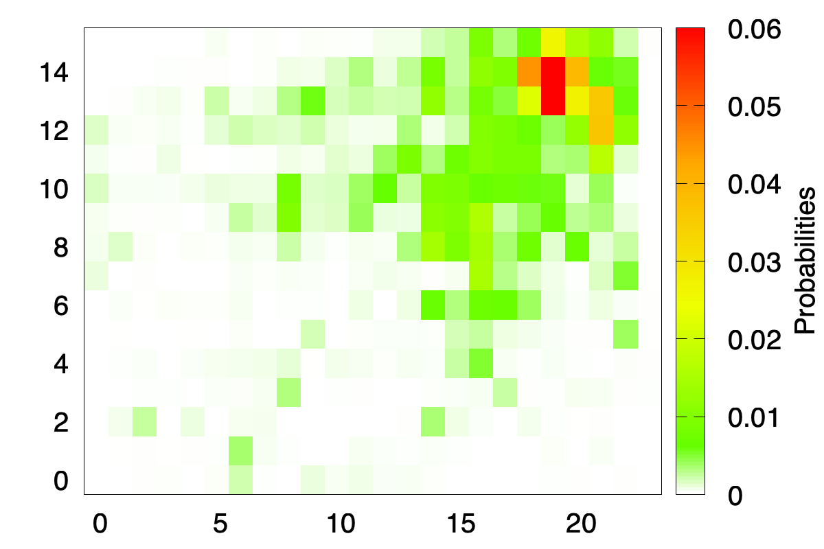
(a) Original

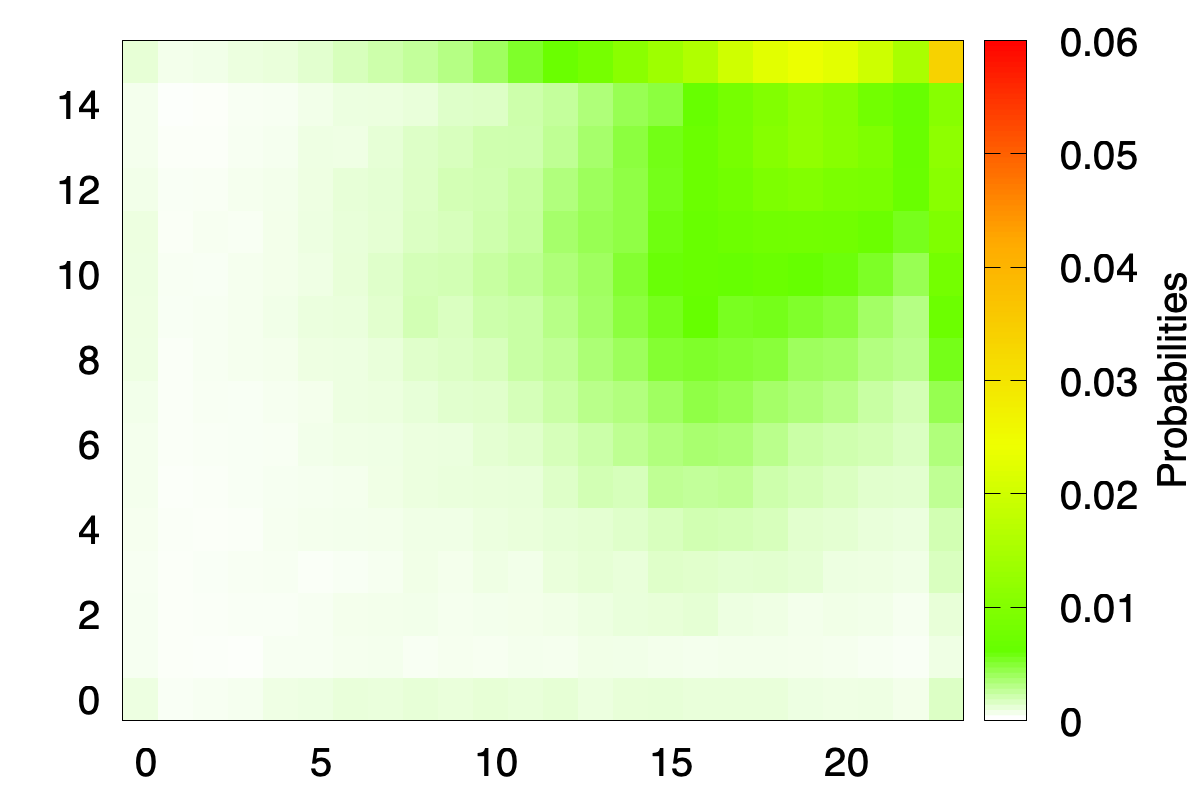
(b) Noisy (TV = 0.4544)

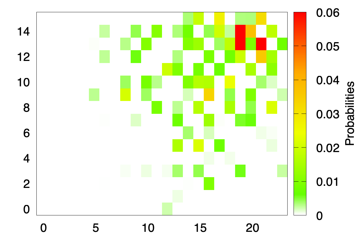
(c) INV-P (TV = 0.4567)

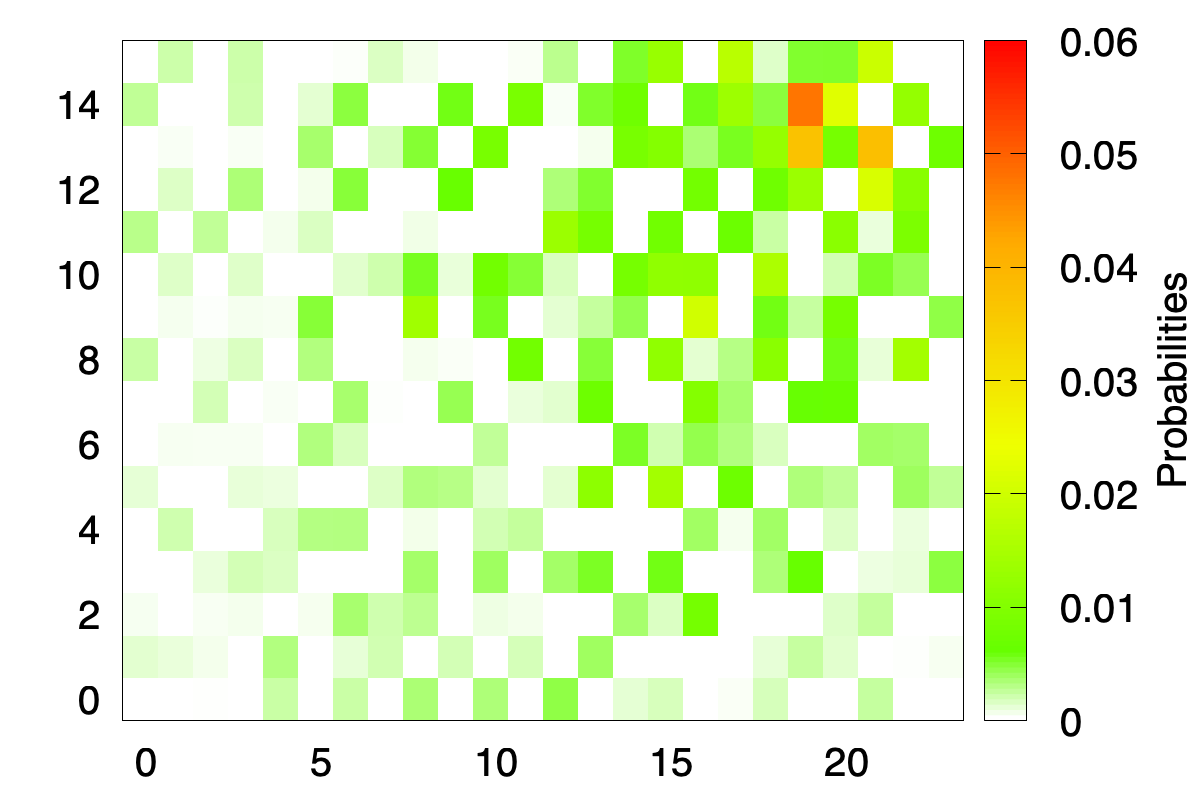
(d) INV-N (TV = 0.4633)

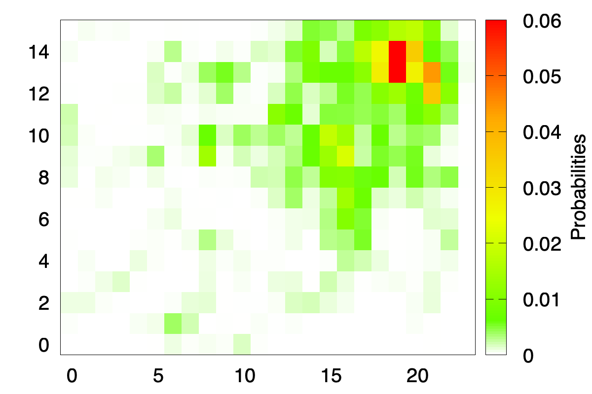
(e) EM (TV = 0.2238)

Figure 9: Estimation of the Gowalla original distribution. The noisy data are produced by a truncated planar geometric mechanism with $\epsilon=1.0$. The shown TV is the total variation distance between the estimation and the original distribution.

Fig. 9 shows the original and noisy distributions on the grid and the distributions estimated by INV-N, INV-P and EM. Also in this case we observe that the EM method outperforms both INV-N and INV-P. We also observe that INV-P is slightly better than INV-N. Finally note that the EM in this experiment yields an MLE that is not interior (in the probability simplex) since many cells have probability $0$ as shown in Fig. 9(e). This is a practical situation that violates the assumption in [10], and hence motivates our revision of the IBU foundations.

IX-C Estimation under various levels of privacy

We perform again the experiment described in Section IX-B, but now we vary the privacy parameter $\epsilon$. We use a range for $\epsilon$ between $0.2$ and $6.0$, and for every value we run the obfuscation-estimation procedure $100$ times to obtain the boxplot in Fig. 10. The estimation quality is measured in terms of the distance from the true distribution (defined by the frequencies of the check-ins in Gowalla). We consider two statistical distances: the Total Variation (TV) and the Earth Mover’s Distance (EMD). As expected, the estimation quality of all methods improves with larger values of $\epsilon$, corresponding to introducing less noise. We observe that EM outperforms INV-N and INV-P, especially at low values of $\epsilon$ (stronger levels of privacy). We also remark that the EMD is more indicative than the TV for comparing distributions on locations: Consider the distributions resulting from INV-P and INV-N in Fig. 9 (where $\epsilon=1$): arguably, the first is more similar to the true distribution than the second one, the latter being quite scattered away from the locations where the probability is accumulated. This qualitative superiority of INV-P over INV-N is reflected by the EMD (Fig. 10(b)), where INV-P is significantly better than INV-N for $\epsilon=1$. On the other hand, in Fig. 10(a), the TV distances for INV-N and INV-P for $\epsilon=1$ on are almost identical (although they differ from the original for opposite reasons: the one from INV-P is too skewed and the one from INV-N is too scattered).

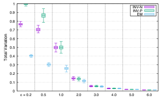
(a) Total variation distance

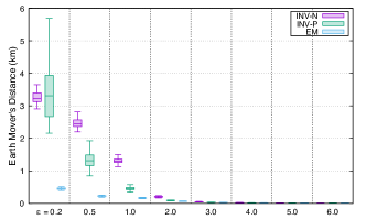
(b) Earth mover’s distance

Figure 10: Statistical distances between the original and the estimated distributions using EM, INV-N, and INV-P. The noisy data are produced using truncated planar geometric mechanisms with various values of $\epsilon$.

Fig. 11 shows the results for the Laplace and exponential mechanisms with the same range of $\epsilon$ as before, and using the TV to measure the estimation quality. Again we observe that EM estimation method substantially outperforms INV-P and INV-N. We also observe that the Laplace mechanism produces a better estimation than the exponential one. This is because the latter introduces larger noise. This is in line with a similar result with respect to the quality of service [23].

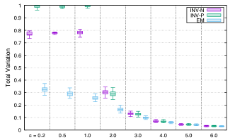
(a) Using the Laplace mechanism

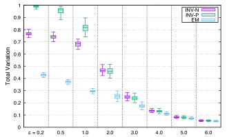
(b) Using the exponential mechanism

Figure 11: The statistical distance, measured by the total variation, between the original and estimated distributions using EM, INV-N, and INV-P. The obfuscation is performed using (a) the Laplace mechanism, and (b) exponential mechanism.

IX-D Estimating distributions obfuscated by $k$-RR mechanisms

Now we use the $k$-RR mechanism described in Section VIII-A to obfuscate the real data, and compare the performance of the three estimation methods on the grid of San Francisco (Fig. 8). We apply the mechanism using various values of $\epsilon$ between $1.0$ and $10$. The results are shown in Fig. 12 in which we plot the TV and EMD distances for the three estimators, at every value of $\epsilon$. Unlike the cases of geometric, Laplace, and exponential mechanisms, we observe that the differences in the performance of estimators are not substantial. Yet, with respect to the TV distance, the EM outperforms both INV-P and INV-N at all the considered values of $\epsilon$. With respect to the EMD, EM and INV-P have almost the same quality and superior to the INV-N.

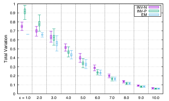
(a) Using the total variation distance

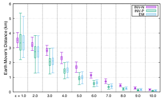
(b) Using the earth mover’s distance

Figure 12: The statistical distance (measured by the total variation in (a), and by the earth mover’s distance in (b)) between the real and estimated distributions using the indicated methods. A $k$-RR mechanism with indicated values of $\epsilon$ is used for obfuscating the user data.

IX-E Estimating distributions obfuscated by Rappor

Rappor is a mechanism built on the idea of randomized response to allow collecting statistics from end-users with differential privacy guarantees [15]. The basic form of this mechanism, called Basic One-Time Rappor maps the space of input values $\mathcal{X}$ to a space $\mathcal{Z}$ of size $2^{|\mathcal{X}|}$. More precisely every user datum $x\in\mathcal{X}$ is encoded in a bit array $B$ of size $|\mathcal{X}|$ in which only one bit $b_{x}$ that uniquely corresponds to $x$ is set to $1$, and other bits are set to $0$. Then every bit $b$ of $B$ is obfuscated independently to yield the same value $b$ with probability $e^{\epsilon/2}/(1+e^{\epsilon/2})$, and $1-b$ with probability $1/(1+e^{\epsilon/2})$. This obfuscation yields a noisy bit vector $B^{\prime}$ that is reported to the server. It can be shown that Rappor satisfies $\epsilon$-local differential privacy.

In order to see the estimation quality of EM with Rappor, we define $\mathcal{X}=\{0,1,\dots,9\}$, which is therefore mapped to $\mathcal{Z}$ of size $2^{10}$. We sample $10^{5}$ inputs (the real data) from two distributions: a binomial with $p=0.5$, and a uniform distribution on $\{3,4,5,6\}$ with probability $0$ to other elements. In each one of these cases, we obfuscate the inputs using a Rappor with $\epsilon=0.5$, and then apply EM to estimate the original distribution. Fig. 13 shows the results of this experiment.

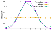
(a) Binomial distribution

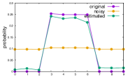
(b) Uniform on $\{3,4,5,6\}$

Figure 13: Using EM to estimate the original distributions on $\{0,1,\dots,9\}$ from noisy data produced by a basic one-time Rappor mechanism with $10^{5}$ user inputs and $\epsilon=0.5$. In (a), the real distribution is binomial. In (b), the real distribution is uniform on $\{3,4,5,6\}$, and assigns probability zero outside this range.

Based on the fact that Rappor uses the binary randomized response obfuscation, the authors of [3] adapted INV-N and INV-P to Rappor. We compare the performance of these methods to that of EM by running the above experiment using the three estimators for $100$ times. In every run we evaluate the total variation (to the original distribution) for every method. Fig. 14 shows the results of this procedure for a range of $\epsilon$.

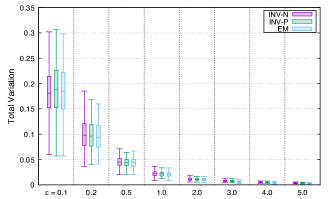
(a) Original data sampled from binomial distribution

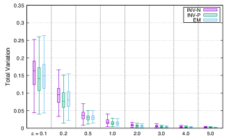
(b) Original data sampled from uniform distribution

Figure 14: The statistical distance between the original and estimated distributions using EM, INV-N, and INV-P, using a Rappor mechanism for obfuscation. Original data of users are sampled from Binomial distribution (a), and from uniform distribution on $\{3,4,5,6\}$ (b).

It can be seen that INV-N, INV-P and EM exhibit almost the same estimation quality. This observation is anticipated from the similar results that we observed with the $k$-RR mechanism in Fig. 12 since both Rappor and $k$-RR are based on the randomized response technique.

X Related work

The papers which are closest to our work have been already discussed in the introduction, so we will not mention them again here.

Besides the local privacy mechanisms considered in this paper, there are many others that have been proposed, aimed at obtaining a good trade-off between privacy and precision of the statistical analyses. Apple uses a method similar to $k$-RR to protect its users’ privacy in applications such as spelling [25]. Bassily and Smith use Random Matrix Projection (BLH) [26], based on ideas from earlier works [27, 11]. Wang et al. [28] have proposed the Optimized Unary Encoding protocol, which builds upon the Basic Rappor, and the Optimized Local Hashing protocol, which is inspired by BLH [26]. Wang et al. [29] use both generalized random response and Basic Rappor for learning weighted histogram.

XI Conclusion

In this paper we have analyzed the iterative Bayesian update (IBU) and we have exhibited various flaws in the underlying theory as presented in the literature. These flaws raise critical questions about the soundness of IBU. Therefore, we have provided new foundations for the IBU, and extended it to a more general local privacy model which allows, for example, the liberty of every user to choose his own mechanism, and to change mechanism while the data are collected. We have also studied various instances of this model.

Finally, we have compared the IBU with the matrix inversion method (INV), showing that, while for mechanisms like $k$-RR and Rappor the results are comparable, with the geo-indistinguishable and the exponential mechanisms the results are clearly in favor of the IBU.

As future work, we also plan to investigate how the choice of the obfuscation mechanism affects the performance of the IBU. This study should lay the basis for identifying mechanisms which optimize the trade-off between privacy and statistical utility.

-A The global convergence theorem

This theorem introduced by Zangwill [30] describes for an iterative algorithm $M$ sufficient conditions that assures a sequence generated by $M$ in some space $\mathcal{C}$ to converge to a set of points $\Gamma\in\mathcal{C}$, called a solution set. Here $M$ is modeled as a set valued function mapping every point in $\mathcal{C}$ to a set of points $M(\boldsymbol{\theta})\subset\mathcal{C}$.

Theorem 1 ([30]).

Consider a sequence $(\boldsymbol{\theta}^{t})_{t\in\mathbb{N}}$ satisfying $\boldsymbol{\theta}^{t+1}\in M(\boldsymbol{\theta}^{t})$, where $M$ is a point-to-set map on $\mathcal{C}$. Let a solution set $\Gamma\subset\mathcal{C}$ be given, and suppose that: (i) all points $\boldsymbol{\theta}^{t}\in\mathcal{C}$ are contained in a compact subset of $\mathcal{C}$; (ii) $M$ is closed at all points of $\mathcal{C}\setminus\Gamma$; (iii) there is a real-valued continuous function $f$ on $\mathcal{C}$ such that

$$f(\boldsymbol{\theta}^{\prime})>f(\boldsymbol{\theta})\quad\forall\boldsymbol{\theta}\not\in\Gamma,\boldsymbol{\theta}^{\prime}\in M(\boldsymbol{\theta}),$$

$$f(\boldsymbol{\theta}^{\prime})\geq f(\boldsymbol{\theta})\quad\forall\boldsymbol{\theta}\in\Gamma,\boldsymbol{\theta}^{\prime}\in M(\boldsymbol{\theta}).$$

Then all the limit points of $(\boldsymbol{\theta}^{t})_{t\in\mathbb{N}}$ are in the solution set $\Gamma$ and $f(\boldsymbol{\theta}^{t})$ converges monotonically to $f(\boldsymbol{\theta})$ for some $\boldsymbol{\theta}\in\Gamma$.

-B planar geometric mechanisms

Suppose that the planar space is discretized by an infinite grid of squared cells, where the side length of each cell is $s$. Let $\mathcal{G}$ be the set of centers of these cells. Then every element of $\mathcal{G}$ is indexed by its coordinates $(i,j)\in\mathbb{Z}^{2}$. For any $\mathcal{X}\subseteq\mathcal{G}$, a planar geometric mechanism (parametrized by $\epsilon,s$) reports a point $z\in\mathcal{G}$ from a real location $x\in\mathcal{X}$ according to the probability

$$P(z|x) =\lambda\,e^{-\epsilon\,\mathbf{d}_{p}(x,z)}\qquad x\in\mathcal{X},z\in\mathcal{G}\$$ (27)

$$\text{where }\lambda =1/\sum_{(i,j)\in\mathbb{Z}^{2}}e^{-\epsilon\,s\,\sqrt{i^{2}+j^{2}}},$$

and $\mathbf{d}_{p}$ is the planar (i.e. Euclidean) distance. For $\mathcal{X}$ finite we can defined a truncated version of the above geometric mechanism. Basically it is obtained by drawing points in $\mathcal{G}$ according to the above distribution and then remapping each of them to its nearest point in $\mathcal{X}$.

-C proofs

We present here the Lemmas and proofs omitted from the paper due to space constraints.

[Derivative of the log-likelihood function]lemmaLQderivatives Consider a parameter space $\mathcal{C}\subset\mathbb{R}^{m}$ and any curve $\boldsymbol{\alpha}:I\to\mathcal{C}$. Then for every $\tau^{\prime}\in I$ it holds that $\frac{dL(\boldsymbol{\alpha}(\tau))}{d\tau}=\frac{dQ(\boldsymbol{\alpha}(\tau)|\boldsymbol{\alpha}(\tau^{\prime}))}{d\tau}$ at $\tau=\tau^{\prime}$.

Proof.

By (4), it is clear that the statement of the proposition is equivalent to $dH(\boldsymbol{\alpha}(\tau)|\boldsymbol{\alpha}(\tau^{\prime}))/d\tau=0$ at $\tau=\tau^{\prime}$, where $H(.|.)$ is defined by (II-B). We start by rewriting $H(.|.)$ in a more convenient form as follows.

$$H(\boldsymbol{\alpha}(\tau)|\boldsymbol{\alpha}(\tau^{\prime}))=-\sum_{w\in\mathcal{S}}\psi_{w}(\tau^{\prime})\log\psi_{w}(\tau)$$

where $\psi_{w}(\tau)=P(S=w|O=o;\boldsymbol{\alpha}(\tau))$ for every $w\in\mathcal{S}$. For more convenience we will write $\psi^{\prime}_{w}=\psi_{w}(\tau^{\prime})$. Now we can evaluate the derivative of $H$ with respect to $\tau$ using the chain rule of derivatives as follows.

$$\frac{dH(\boldsymbol{\alpha}(\tau)|\boldsymbol{\alpha}(\tau^{\prime}))}{d\tau}=\sum_{s\in\mathcal{S}}\frac{\partial H}{\partial\psi_{s}}\frac{d\psi_{s}}{d\tau}.$$ (28)

Using the definition of $H$ and the linearity of $\partial/{\partial\psi_{s}}$ we have

$$\frac{\partial H}{\partial\psi_{s}}=-\sum_{w\in\mathcal{S}}\frac{\partial}{\partial\psi_{s}}\left(\psi^{\prime}_{w}\log\psi_{w}\right)=-\psi^{\prime}_{s}/\psi_{s}.$$

By substituting the above expression in (28), and observing that at $\tau=\tau^{\prime}$ we have $\psi_{s}=\psi^{\prime}_{s}$ for all $s\in\mathcal{S}$, we obtain

$$\frac{dH(\boldsymbol{\alpha}(\tau)|\boldsymbol{\alpha}(\tau^{\prime}))}{d\tau}\Big{|}_{\tau=\tau^{\prime}}=-\sum_{s\in\mathcal{S}}\frac{d\psi_{s}}{d\tau}=0$$

where the last equality follows from $\sum_{s\in\mathcal{S}}\psi_{s}(\tau)=1$. ∎

*

Proof.

We prove the theorem by showing that the conditions of Theorem 1 are satisfied. Condition (i) is clearly satisfied. Condition (ii) is satisfied by the continuity of $Q(\boldsymbol{\theta}|\boldsymbol{\theta}^{\prime})$ in both $\boldsymbol{\theta},\boldsymbol{\theta}^{\prime}$ as noted by [10]. For Condition (iii) we define $f(.)=L(.)$ which is continuous, and proceed to prove the two parts of (iii) as follows. The map $M_{\textit{em}}$ of the EM algorithm is defined for every $\boldsymbol{\theta}^{\prime}\in\mathcal{C}$ (by the M-step) as follows.

$$M_{\textit{em}}(\boldsymbol{\theta}^{\prime})=\{\boldsymbol{\theta}\in\mathcal{C}:Q(\boldsymbol{\theta}|\boldsymbol{\theta}^{\prime})\geq Q(\boldsymbol{\theta}^{\prime\prime}|\boldsymbol{\theta}^{\prime})\,\forall\boldsymbol{\theta}^{\prime\prime}\in\mathcal{C}\}.$$ (29)

It is clear that the definition of $M_{\textit{em}}$ together with (5) implies that $L(\boldsymbol{\theta})\geq L(\boldsymbol{\theta}^{\prime})$ for all $\boldsymbol{\theta}^{\prime}\in\mathcal{C}$ and $\boldsymbol{\theta}\in M_{\textit{em}}(\boldsymbol{\theta}^{\prime})$, hence satisfying the second part of Condition (iii) in Theorem 1. It remains to prove first part of (iii) with respect to $M_{\textit{em}},\Gamma$. Consider any $\boldsymbol{\theta}^{\prime}\not\in\Gamma$. Then by Definition 3 of $\Gamma$, there must be a curve $\boldsymbol{\alpha}:I\to\mathcal{C}$ such that $\boldsymbol{\theta}^{\prime}=\boldsymbol{\alpha}(\tau^{\prime})$ for some $\tau^{\prime}\in I$ and $\boldsymbol{\theta}^{\prime}$ is neither stationary nor a local maximizer along $\boldsymbol{\alpha}$. This means

$$|dL(\boldsymbol{\alpha}(\tau))/d\tau|_{\tau=\tau^{\prime}}=c>0,$$ (30)

$$\forall\delta>0\,\exists\tau^{\prime\prime}\in I:0<|\tau^{\prime\prime}-\tau^{\prime}|<\delta,$$

$$\qquad\qquad\qquad\qquad L(\boldsymbol{\alpha}(\tau^{\prime\prime}))>L(\boldsymbol{\alpha}(\tau^{\prime})).$$ (31)

Using the definition of derivatives and that $|\lim_{\tau\to\tau^{\prime}}f(\tau)|=\lim_{\tau\to\tau^{\prime}}|f(\tau)|$ for any function $f$, we imply from (30) that

$$\lim_{\tau\to\tau^{\prime}}\Big{|}\frac{L(\boldsymbol{\alpha}(\tau))-L(\boldsymbol{\alpha}(\tau^{\prime}))}{\tau-\tau^{\prime}}\Big{|}=c.$$ (32)

It also follows from Proposition -C and the definition of derivatives that

$$\lim_{\tau\to\tau^{\prime}}\Big{(}\frac{Q(\boldsymbol{\alpha}(\tau)|\boldsymbol{\alpha}(\tau^{\prime}))-Q(\boldsymbol{\alpha}(\tau^{\prime})|\boldsymbol{\alpha}(\tau^{\prime}))}{\tau-\tau^{\prime}} -$$

$$\frac{L(\boldsymbol{\alpha}(\tau))-L(\boldsymbol{\alpha}(\tau^{\prime}))}{\tau-\tau^{\prime}}\Big{)} =0.$$ (33)

Choose any $\epsilon$ such that $0<\epsilon<c/2$. Then by the definition of limits there are $\delta_{\epsilon}>0$ and (by (31)) $\tau^{\prime\prime}\in I$ with $|\tau^{\prime\prime}-\tau^{\prime}|<\delta_{\epsilon}$ and $L(\boldsymbol{\alpha}(\tau^{\prime\prime}))>L(\boldsymbol{\alpha}(\tau^{\prime}))$ such that

$$-\epsilon<\frac{L(\boldsymbol{\alpha}(\tau^{\prime\prime}))-L(\boldsymbol{\alpha}(\tau^{\prime}))}{|\tau^{\prime\prime}-\tau^{\prime}|}-c<\epsilon,$$ (34)

$$-\epsilon<\frac{Q(\boldsymbol{\alpha}(\tau^{\prime\prime})|\boldsymbol{\alpha}(\tau^{\prime}))-Q(\boldsymbol{\alpha}(\tau^{\prime})|\boldsymbol{\alpha}(\tau^{\prime}))}{|\tau^{\prime\prime}-\tau^{\prime}|}-$$

$$\qquad\qquad\qquad\qquad\frac{L(\boldsymbol{\alpha}(\tau^{\prime\prime}))-L(\boldsymbol{\alpha}(\tau^{\prime}))}{|\tau^{\prime\prime}-\tau^{\prime}|}<\epsilon$$ (35)

Inequalities in (34) follow from (32) with the substitution $|L(\boldsymbol{\alpha}(\tau^{\prime\prime}))-L(\boldsymbol{\alpha}(\tau^{\prime}))|=L(\boldsymbol{\alpha}(\tau^{\prime\prime}))-L(\boldsymbol{\alpha}(\tau^{\prime}))$ since $L(\boldsymbol{\alpha}(\tau^{\prime\prime}))>L(\boldsymbol{\alpha}(\tau^{\prime}))$. Inequalities (35) follow from (-C). Now from the left inequalities in both (34) and (35) we obtain respectively

$$(c-\epsilon)\,|\tau^{\prime\prime}-\tau^{\prime}|<L(\boldsymbol{\alpha}(\tau^{\prime\prime}))-L(\boldsymbol{\alpha}(\tau^{\prime})),$$

$$L(\boldsymbol{\alpha}(\tau^{\prime\prime}))-L(\boldsymbol{\alpha}(\tau^{\prime}))-\epsilon|\tau^{\prime\prime}-\tau^{\prime}|<$$

$$\qquad\qquad\qquad\qquad Q(\boldsymbol{\alpha}(\tau^{\prime\prime})|\boldsymbol{\alpha}(\tau^{\prime}))-Q(\boldsymbol{\alpha}(\tau^{\prime})|\boldsymbol{\alpha}(\tau^{\prime})).$$

By substituting the first inequality in the second one, we obtain

$$(c-2\epsilon)|\tau^{\prime\prime}-\tau^{\prime}|<Q(\boldsymbol{\alpha}(\tau^{\prime\prime})|\boldsymbol{\alpha}(\tau^{\prime}))-Q(\boldsymbol{\alpha}(\tau^{\prime})|\boldsymbol{\alpha}(\tau^{\prime}))$$

which implies that $Q(\boldsymbol{\alpha}(\tau^{\prime\prime})|\boldsymbol{\alpha}(\tau^{\prime}))>Q(\boldsymbol{\alpha}(\tau^{\prime})|\boldsymbol{\alpha}(\tau^{\prime}))$ because $c>2\epsilon$. Since $\boldsymbol{\theta}^{\prime}=\boldsymbol{\alpha}(\tau^{\prime})$ and $\boldsymbol{\alpha}(\tau^{\prime\prime})\in\mathcal{C}$ then the above inequality together with the definition of $M_{\textit{em}}$ in (29) imply that for all $\boldsymbol{\theta}\in M_{\textit{em}}(\boldsymbol{\theta}^{\prime})$ we have $Q(\boldsymbol{\theta}|\boldsymbol{\theta}^{\prime})>Q(\boldsymbol{\theta}^{\prime}|\boldsymbol{\theta}^{\prime})$ which implies by (5) that $L(\boldsymbol{\theta})>L(\boldsymbol{\theta}^{\prime})$. Thus the first part of condition (iii) in Theorem 1 is satisfied. ∎

*

Proof.

By Definition 3 of $\Gamma$, it is clear that every global maximizer of $L(.)$ is in $\Gamma$. We show in the following that every element $\boldsymbol{\theta}\in\Gamma$ is a global maximizer. Consider any $\boldsymbol{\theta}\in\Gamma$ and $\boldsymbol{\phi}\in\mathcal{C}$, and assume (for a contradiction) that $L(\boldsymbol{\theta})<L(\boldsymbol{\phi})$. Consider the curve $\boldsymbol{\alpha}(\tau)=(1-\tau)\boldsymbol{\theta}+\tau\boldsymbol{\phi}$ for $\tau\in[0,1]$ which is the straight line segment between $\boldsymbol{\theta},\boldsymbol{\phi}$. Note that $\boldsymbol{\theta}=\boldsymbol{\alpha}(0),\boldsymbol{\phi}=\boldsymbol{\alpha}(1)$, and also $\boldsymbol{\alpha}:[0,1]\to\mathcal{C}$ since $\mathcal{C}$ is convex. Now it can be seen that $\boldsymbol{\theta}$ is not stationary along $\boldsymbol{\alpha}$ since

$$\frac{dL(\boldsymbol{\alpha}(\tau))}{d\tau}\big{|}_{\tau\to 0}=\lim_{\tau\to 0}\frac{L((1-\tau)\boldsymbol{\theta}+\tau\boldsymbol{\phi})-L(\boldsymbol{\theta})}{\tau}\geq$$

$$\lim_{\tau\to 0}\frac{(1-\tau)L(\boldsymbol{\theta})+\tau L(\boldsymbol{\phi})-L(\boldsymbol{\theta})}{\tau}=L(\boldsymbol{\phi})-L(\boldsymbol{\theta})>0$$

where the first inequality above follows from the concavity of $L(.)$, and the last inequality follows from the assumption $L(\boldsymbol{\theta})<L(\boldsymbol{\phi})$. We also show in the following that $\boldsymbol{\theta}$ is not a local maximizer along $\boldsymbol{\alpha}$. Consider any $0<\delta$, and choose any $\tau$ such that $0<\tau<\min\{\delta,1\}$. Then $\tau\in[0,1]$ and $|\tau-0|<\delta$. Now by the concavity of $L(.)$ it holds that

$$L(\boldsymbol{\alpha}(\tau))\geq(1-\tau)L(\boldsymbol{\theta})+\tau L(\boldsymbol{\phi})>$$

$$\qquad\qquad\qquad\qquad(1-\tau)L(\boldsymbol{\theta})+\tau L(\boldsymbol{\theta})=L(\boldsymbol{\theta})$$

where the second (strict) inequality follows from the assumption that $L(\boldsymbol{\theta})<L(\boldsymbol{\phi})$ and that $\tau>0$. Therefore $\boldsymbol{\theta}$ is not a local maximizer. We conclude that $\boldsymbol{\theta}$ is neither stationary nor a local maximizer along $\boldsymbol{\alpha}$, contradicting that $\boldsymbol{\theta}\in\Gamma$. ∎

*

Proof.

Since $\{X^{i}:1\leq i\leq n\}$ are mutually independent, we can write $Q(.|.)$ as follows

$$Q(\boldsymbol{\theta}|\boldsymbol{\theta}^{t}) =\sum_{i=1}^{n}\mathbf{E}\left[\log P(X^{i},Z^{i}|\boldsymbol{\theta})|Z^{i}=\boldsymbol{z}^{i};\boldsymbol{\theta}^{t}\right]$$

$$=\sum_{i=1}^{n}\sum_{x\in\mathcal{X}}P(X^{i}=x|Z^{i}=\boldsymbol{z}^{i};\boldsymbol{\theta}^{t})$$

$$\qquad\qquad\qquad\qquad\log P(X^{i}=x,Z^{i}=\boldsymbol{z}^{i}|\boldsymbol{\theta})$$

$$=\sum_{i=1}^{n}\sum_{x\in\mathcal{X}}P(X^{i}=x|Z^{i}=\boldsymbol{z}^{i};\boldsymbol{\theta}^{t})$$

$$\qquad\qquad\qquad\qquad\log\theta_{x}P(Z^{i}=\boldsymbol{z}^{i}|X^{i}=x)$$

$$=\sum_{x\in\mathcal{X}}\psi_{x}(\boldsymbol{z},\boldsymbol{\theta}^{t})\log\theta_{x}+$$

$$\qquad\qquad\sum_{x\in\mathcal{X}}\sum_{i=1}^{n}P(X^{i}=x|Z^{i}=\boldsymbol{z}^{i};\boldsymbol{\theta}^{t})\log g_{xi}.$$

where the last equality follows from the definition of $\psi_{x}(\boldsymbol{z},\boldsymbol{\theta}^{t})$ and Definition 4 for $g_{xi}$. ∎

*

Proof.

Since we require every $\boldsymbol{\theta}$ to satisfy the constraint $\sum_{x}\theta_{x}=1$, we use the Lagrange multiplier $\lambda$ to preserve this constraint and therefore maximize the following function

$$\mathcal{L}(\boldsymbol{\theta},\lambda)=Q(\boldsymbol{\theta}|\boldsymbol{\theta}^{t})+\lambda(\sum_{x\in\mathcal{X}}\theta_{x}-1).$$

The above function is maximum at $\boldsymbol{\theta},\lambda$ that satisfy $\partial\mathcal{L}/\partial\theta_{x}=0$ for all $x\in\mathcal{X}$, and also $\partial\mathcal{L}/\partial\lambda=0$. Then, by Theorem V-B we obtain $\partial\mathcal{L}/\partial\theta_{x}=\psi_{x}(\boldsymbol{z},\boldsymbol{\theta}^{t})/\theta_{x}+\lambda=0$ which yields $\theta_{x}=-\psi_{x}(\boldsymbol{z},\boldsymbol{\theta}^{t})/\lambda$ for all $x\in\mathcal{X}$. From the condition $\partial\mathcal{L}/\partial\lambda=0$ we obtain $\lambda=-\sum_{x\in\mathcal{X}}\psi_{x}(\boldsymbol{z},\boldsymbol{\theta}^{t})=-n$ where the last equality follows from the definition of $\psi_{x}(\boldsymbol{z},\boldsymbol{\theta}^{t})$ in Theorem V-B. Thus $\mathcal{L}(\boldsymbol{\theta},\lambda)$ is maximized at $\boldsymbol{\theta}$ with $\theta_{x}=\psi_{x}(\boldsymbol{z},\boldsymbol{\theta}^{t})/n$ for all $x\in\mathcal{X}$. The proof is finally completed by substituting $\psi_{x}(\boldsymbol{z},\boldsymbol{\theta}^{t})$ with its definition in Theorem V-B. ∎

*

Proof.

From the definition of $\mathcal{C}^{\prime},\mathcal{C}$ it is clear that $\mathcal{C}^{\prime}\subset\mathcal{C}\subset\mathbb{R}^{|\mathcal{X}|}$. Then by the Bolzano–Weierstrass theorem, $\mathcal{C}^{\prime}$ is compact if and only if it is bounded in $\mathbb{R}^{|\mathcal{X}|}$ and closed. It is clear that $\mathcal{C}^{\prime}$ is bounded since $\mathcal{C}$ is. It is also closed, i.e. containing its limit points as follows. Every limit point $\boldsymbol{\theta}^{*}$ of $\mathcal{C}^{\prime}$ is the limit of some sequence $(\boldsymbol{\theta}^{t})_{t\in\mathbb{N}}$ sampled from $\mathcal{C}^{\prime}\setminus\boldsymbol{\theta}^{*}$, i.e. $\lim_{t\to\infty}\boldsymbol{\theta}^{t}=\boldsymbol{\theta}^{*}$. Here it can be seen from the definitions of $\mathcal{C}^{\prime},\mathcal{C}$ that $\theta^{*}_{x}\geq 0$ for all $x\in\mathcal{X}$ and $\sum_{x\in\mathcal{X}}\theta^{*}_{x}=1$. It also follows that $L^{-}\leq\lim_{t\to\infty}L(\boldsymbol{\theta}^{t})=L(\boldsymbol{\theta}^{*})$ where the last equality holds by the continuity of $L(.)$ on $\mathcal{C}$, and therefore on $\mathcal{C}^{\prime}$. Thus $\boldsymbol{\theta}^{*}\in\mathcal{C}^{\prime}$, hence $\mathcal{C}^{\prime}$ is closed. ∎

*

Proof.

$L(.)=\sum_{i=1}^{n}L_{i}(.)$ is concave because $L_{i}(.)$ is concave by (10) for all $i$. $\mathcal{C}$ is convex. In fact for every two distributions $\boldsymbol{\theta},\boldsymbol{\phi}\in\mathcal{C}$ and every $\tau\in[0,1]$, the distribution $\boldsymbol{\theta}^{\prime}=(1-\tau)\boldsymbol{\theta}+\tau\boldsymbol{\phi}$ is in $\mathcal{C}$ because $\boldsymbol{\theta}^{\prime}$ is a distribution and $L(\boldsymbol{\theta}^{\prime})\geq(1-\tau)L(\boldsymbol{\theta})+\tau L(\boldsymbol{\phi})>-\infty$ where the first inequality follows from the concavity of $L(.)$ and the second from $\boldsymbol{\theta},\boldsymbol{\phi}\in\mathcal{C}$. ∎

*

Proof.

We show first that $(\boldsymbol{\theta}^{t})_{t\in\mathbb{N}}$ is contained in a compact subset $\mathcal{C}^{\prime}$ of $\mathcal{C}$. Let $\mathcal{C}^{\prime}=\{\boldsymbol{\theta}\in\mathcal{C}:L(\boldsymbol{\theta})\geq L(\boldsymbol{\theta}^{0})\}$. Since $L(\boldsymbol{\theta}^{0})>-\infty$ it follows from Lemma 1, that $\mathcal{C}^{\prime}$ is compact. Since also $L(\boldsymbol{\theta}^{t})$ is monotonically increasing by Theorem V-B and (5), we have $L(\boldsymbol{\theta}^{t})\geq L(\boldsymbol{\theta}^{0})$ for all $t\in\mathbb{N}$. Therefore the generated sequence $(\boldsymbol{\theta}^{t})_{t\in\mathbb{N}}$ is contained in $\mathcal{C}^{\prime}$. Since $L(.)$ is continuous on $\mathcal{C}$ and $Q(.|.)$ is continuous with respect to its two arguments (Theorem V-B), it follows from Theorem 3 that $L(\boldsymbol{\theta}^{t})$ converges to $L(\hat{\boldsymbol{\theta}})$ for some $\hat{\boldsymbol{\theta}}\in\Gamma$. Then by Lemma V-D, $L(.)$ is concave and $\mathcal{C}$ is convex; and therefore $\Gamma$ is exactly the set of global maximizers by Theorem 3. ∎

*

Proof.

Let $P(\boldsymbol{z}|\boldsymbol{\theta})$ denote the probability of $\boldsymbol{z}$ with respect to a distribution $\boldsymbol{\theta}$ on $\mathcal{X}$. Then for all distributions $\boldsymbol{\theta}$ it holds that $P(\boldsymbol{z}|\boldsymbol{\theta})$ is tightly upper-bounded as follows

$$P(\boldsymbol{z}|\boldsymbol{\theta})=\sum_{x\in\mathcal{X}}\theta_{x}\,P(\boldsymbol{z}|X=x)\leq\max_{x\in\mathcal{X}}P(\boldsymbol{z}|x).$$

Now define $M$ to be the above upper bound, i.e. $M=\max_{x\in\mathcal{X}}P(\boldsymbol{z}|x)$; then it holds for any distribution $\boldsymbol{\theta}$ that

$$M-P(\boldsymbol{z}|\boldsymbol{\theta}) =M\sum_{x\in\mathcal{X}}\theta_{x}-\sum_{x\in\mathcal{X}}\theta_{x}\,P(\boldsymbol{z}|x)$$

$$=\sum_{x\in\mathcal{X}}(M-P(\boldsymbol{z}|x))\theta_{x}\geq 0.$$

It follows from the above inequality that $P(\boldsymbol{z}|\boldsymbol{\theta})$ attains the maximum value $M$ if and only if $\theta_{x}=0$ for all $x$ satisfying $M-P(\boldsymbol{z}|x)>0$, i.e. $x\not\in\mathcal{X}$. This condition is equivalent to that given in the theorem statement. ∎

*

Proof.

Let $\mathcal{C}$ be the set of all probability distributions $\boldsymbol{\theta}$ on $\mathcal{X}$ with finite log-likelihood, i.e. $L(\boldsymbol{\theta})>-\infty$. Let also $\mathcal{C}^{\prime}=\{\boldsymbol{\theta}\in\mathcal{C}:L(\boldsymbol{\theta})\geq L(\boldsymbol{\theta}^{\prime})\}$. Then it follows from Lemma 1 that $\mathcal{C}^{\prime}$ is compact. Since also $L(.)$ is continuous on $\mathcal{C}^{\prime}$ it has a global maximizer in $\mathcal{C}^{\prime}$ (by the extreme value theorem). Therefore $L(.)$ has a global maximizer in $\mathcal{C}$. Now we show under the condition stated in the theorem that $L(.)$ is also strictly concave on $\mathcal{C}$. Since $L(\boldsymbol{\theta})=\sum_{i=1}^{n}L_{i}(\boldsymbol{\theta})$, we can split this sum into two parts as follows.

$$L(\boldsymbol{\theta})=\sum_{i\in\mathcal{I}^{\prime}}L_{i}(\boldsymbol{\theta})+\sum_{i\in(\mathcal{I}\setminus\mathcal{I}^{\prime})}L_{i}(\boldsymbol{\theta}).$$ (36)

Now let $\boldsymbol{\theta},\boldsymbol{\phi}$ be any two nonidentical distributions on $\mathcal{X}$, and consider any $0<\gamma<1$. Then by (10) it holds for every $i\in\mathcal{I}^{\prime}$ that

$$L_{i}(\gamma\boldsymbol{\theta}+(1-\gamma)\boldsymbol{\phi})=\log\sum_{u\in\mathcal{X}}(\gamma\theta_{u}+(1-\gamma)\phi_{u})g_{ui}$$

$$\qquad\qquad=\log\left(\gamma\sum_{u\in\mathcal{X}}\theta_{u}g_{ui}+(1-\gamma)\sum_{u\in\mathcal{X}}\phi_{u}g_{ui}\right)$$

$$\qquad\qquad\geq\gamma\log\sum_{u\in\mathcal{X}}\theta_{u}g_{ui}+(1-\gamma)\log\sum_{u\in\mathcal{X}}\phi_{u}g_{ui}$$

$$\qquad\qquad=\gamma\,L_{i}(\boldsymbol{\theta})+(1-\gamma)\,L_{i}(\boldsymbol{\phi})$$

where the above inequality follows from the Jensen inequality and the concavity of the $\log(.)$. The inequality is strict equality if and only if

$$\sum_{u\in\mathcal{X}}\theta_{u}g_{ui}=\sum_{u\in\mathcal{X}}\phi_{u}g_{ui}.$$ (37)

Therefore

$$\sum_{i\in\mathcal{I}^{\prime}}L_{i}(\gamma\boldsymbol{\theta}+(1-\gamma)\boldsymbol{\phi})\geq\gamma\sum_{i\in\mathcal{I}^{\prime}}\,L_{i}(\boldsymbol{\theta})+(1-\gamma)\,\sum_{i\in\mathcal{I}^{\prime}}L_{i}(\boldsymbol{\phi})$$ (38)

where the above inequality is equality if and only if (37) is satisfied for all $i\in\mathcal{I}^{\prime}$, i.e. $(\boldsymbol{\theta}-\boldsymbol{\phi})\,\boldsymbol{G}(\mathcal{I}^{\prime})=\boldsymbol{0}$. Therefore if this condition is never satisfied for every non-identical $\boldsymbol{\theta},\boldsymbol{\phi}$ the inequality in (38) strict, which implies by (36) that $L(.)$ is strictly concave on $\mathcal{C}$ which is convex (Lemma V-D). Therefore the global maximizer of $L(.)$ on $\mathcal{C}$ is unique. ∎

*

Proof.

Let $\mathcal{X}=\{x_{1},x_{2},\dots,x_{m}\}$ be the values reported by the $k$-RR. We define the set $\mathcal{I}^{\prime}$ to include for every $x\in\mathcal{X}$ an index (in the sequence of outputs) at which the value $x$ is observed. Then both the rows and columns of $\boldsymbol{G}(\mathcal{I}^{\prime})$ correspond to the $m$ elements of $\mathcal{X}$. Let $a=e^{\epsilon}/(1-k+e^{\epsilon})$, $b=1/(1-k+e^{\epsilon})$, and $C_{i}$ be the $i$-th column of $\boldsymbol{G}(\mathcal{I}^{\prime})$. Then by (20)

$$C_{i}=[b,b,\dots,b,a,b,b,\dots,b]^{T}$$

in which the $i$-th entry is $a$ and every other entry is $b$. Let $\boldsymbol{1}$ be the column vector having all entries equal to $1$. We first show that any row vector $\boldsymbol{v}$ satisfying $\boldsymbol{v}\,\boldsymbol{G}(\mathcal{I}^{\prime})=\boldsymbol{0}$, $\boldsymbol{v}\boldsymbol{1}=0$ must be equal to $\boldsymbol{0}$. These constraints imply for every $i=1,2,\dots,m$ that $\boldsymbol{v}\,(C_{i}-b\boldsymbol{1})=\boldsymbol{0}$ which means that $v_{i}=0$ for every $i$, i.e. $\boldsymbol{v}=\boldsymbol{0}$. We know that any two distributions $\boldsymbol{\theta},\boldsymbol{\phi}$ satisfy $(\boldsymbol{\theta}-\boldsymbol{\phi})\boldsymbol{1}=0$. Therefore if they also satisfy $(\boldsymbol{\theta}-\boldsymbol{\phi})\,\boldsymbol{G}(\mathcal{I}^{\prime})=\boldsymbol{0}$ they must satisfy $\boldsymbol{\theta}-\boldsymbol{\phi}=\boldsymbol{0}$, i.e. must be identical, which implies by Theorem VIII that the MLE on $\mathcal{X}$ is unique. ∎

*

Proof.

Let $\mathcal{X}=\{x_{1},x_{2},\dots,x_{m}\}$ be the set of reported values. We define the set $\mathcal{I}^{\prime}$ to contain for every $x\in\mathcal{X}$ an index (in the sequence of outputs) at which the value $x$ is observed. Then both the rows and columns of $\boldsymbol{G}(\mathcal{I}^{\prime})$ correspond to the elements of $\mathcal{X}$. We assume without loss of generality that $x_{1}<x_{2}<\dots<x_{m}$. Then using (21), and letting $\alpha=e^{-\epsilon}$ we can write $\boldsymbol{G}(\mathcal{I}^{\prime})$ as

$$\boldsymbol{G}(\mathcal{I}^{\prime})=c\,\begin{bmatrix}1&\alpha^{x_{2}-x_{1}}&\alpha^{x_{3}-x_{1}}&\dots&\alpha^{x_{m}-x_{1}}\\ \alpha^{x_{2}-x_{1}}&1&\alpha^{x_{3}-x_{2}}&\dots&\alpha^{x_{m}-x_{2}}\\ \alpha^{x_{3}-x_{1}}&\alpha^{x_{3}-x_{2}}&1&\dots&\alpha^{x_{m}-x_{3}}\\ \vdots&\vdots&\vdots&\ddots&\vdots\\ \alpha^{x_{m}-x_{1}}&\alpha^{x_{m}-x_{2}}&\alpha^{x_{m}-x_{3}}&\dots&1\end{bmatrix}.$$

We show that any vector $\boldsymbol{v}$ satisfying $\boldsymbol{v}\,\boldsymbol{G}(\mathcal{I}^{\prime})=\boldsymbol{0}$ must be zero. This is a system of $m$ linear equations in which the $i$-th one corresponds to the $i$-th column $C_{i}$ of the above matrix as $\boldsymbol{v}\,C_{i}=0$. It is easy to see that $\boldsymbol{v}\,(C_{1}-\alpha^{(x_{2}-x_{1})}C_{2})=0$ yields $v_{1}=0$. Using this together with $\boldsymbol{v}\,(C_{2}-\alpha^{(x_{3}-x_{2})}C_{3})=0$ yields $v_{2}=0$. Repeating this procedure inductively on every successive two columns yields that $v_{i}=0$ for all $i\leq m$. Therefore any two distributions $\boldsymbol{\theta},\boldsymbol{\phi}$ satisfying $(\boldsymbol{\theta}-\boldsymbol{\phi})\,\boldsymbol{G}(\mathcal{I}^{\prime})=\boldsymbol{0}$ must be identical, which implies by Theorem VIII that the MLE on $\mathcal{X}$ is unique. ∎

*

Proof.

The proof is similar to that of Corollary 21 with the only difference is that every column in $\boldsymbol{G}(\mathcal{I}^{\prime})$ is scaled by $c_{x_{i}}/c$ where $x_{i}$ for $i=1,2,\dots,m$ are the observed values, and $c_{x_{i}}$ is given by (26). ∎

References

- [1] C. Dwork and A. Roth, “The algorithmic foundations of differential privacy,” Foundations and Trends® in Theor. Comp. Sci., vol. 9, no. 3–4, pp. 211–407, 2014.
- [2] R. Agrawal, R. Srikant, and D. Thomas, “Privacy Preserving OLAP,” in Proceedings of the 24th ACM SIGMOD Int. Conf. on Management of Data, ser. SIGMOD ’05. ACM, 2005, pp. 251–262.
- [3] P. Kairouz, K. Bonawitz, and D. Ramage, “Discrete distribution estimation under local privacy,” in Proceedings of the 33rd International Conference on International Conference on Machine Learning - Volume 48, ser. ICML’16. JMLR.org, 2016, pp. 2436–2444.
- [4] D. Agrawal and C. C. Aggarwal, “On the design and quantification of privacy preserving data mining algorithms,” in Proc. of PODS, ser. PODS ’01. ACM, 2001, pp. 247–255.
- [5] T. Murakami, H. Hino, and J. Sakuma, “Toward distribution estimation under local differential privacy with small samples,” PoPETs, vol. 2018, no. 3, pp. 84–104, 2018.
- [6] M. S. Alvim, K. Chatzikokolakis, C. Palamidessi, and A. Pazii, “Local differential privacy on metric spaces: Optimizing the trade-off with utility,” in Proc. of CSF. IEEE Computer Society, 2018, pp. 262–267.
- [7] L. Kacem and C. Palamidessi, “Geometric noise for locally private counting queries,” in Proc. of PLAS. ACM, 2018, pp. 13–16.
- [8] S. Oya, C. Troncoso, and F. Pérez-González, “A tabula rasa approach to sporadic location privacy,” in Proceedings of S& P., vol. abs/1809.04415, 2019.
- [9] S. Oya, “A Statistical Approach to the Design of Privacy-Preserving Services,” Ph.D. dissertation, Universida de Vigo, 2019.
- [10] C. F. J. Wu, “On the convergence properties of the EM algorithm,” The Annals of Statistics, vol. 11, no. 1, pp. 95–103, 1983.
- [11] J. C. Duchi, M. I. Jordan, and M. J. Wainwright, “Local privacy and statistical minimax rates,” in Proc. of FOCS. IEEE Computer Society, 2013, pp. 429–438.
- [12] P. Kairouz, S. Oh, and P. Viswanath, “Extremal mechanisms for local differential privacy,” The JMLR, vol. 17, no. 1, pp. 492–542, 2016.
- [13] K. Chatzikokolakis, M. E. Andrés, N. E. Bordenabe, and C. Palamidessi, “Broadening the scope of Differential Privacy using metrics,” in Proc. of PETS, ser. LNCS, vol. 7981. Springer, 2013, pp. 82–102.
- [14] M. E. Andrés, N. E. Bordenabe, K. Chatzikokolakis, and C. Palamidessi, “Geo-indistinguishability: differential privacy for location-based systems,” in Proc. of CCS. ACM, 2013, pp. 901–914.
- [15] Ú. Erlingsson, V. Pihur, and A. Korolova, “RAPPOR: randomized aggregatable privacy-preserving ordinal response,” in Proc. of CCS. ACM, 2014, pp. 1054–1067.
- [16] A. P. Dempster, N. M. Laird, and D. B. Rubin, “Maximum likelihood from incomplete data via the EM algorithm,” Journal of the Royal Statistical Society. Series B (Methodological), vol. 39, no. 1, pp. 1–38, 1977.
- [17] G. McLachlan and T. Krishnan, The EM algorithm and extensions, 2nd ed., ser. Wiley series in probability and statistics. Hoboken, NJ: Wiley, 2008.
- [18] T. M. Cover and J. A. Thomas, Elements of Information Theory, 2nd ed. J. Wiley & Sons, Inc., 2006.
- [19] M. Boreale, F. Pampaloni, and M. Paolini, “Asymptotic information leakage under one-try attacks,” Mathematical Structures in Computer Science, vol. 25, no. 02, pp. 292–319, 2015.
- [20] S. L. Warner, “Randomized response: A survey technique for eliminating evasive answer bias,” Journal of the American Statistical Association, vol. 60, no. 309, pp. 63–69, 1965.
- [21] A. Ghosh, T. Roughgarden, and M. Sundararajan, “Universally utility-maximizing privacy mechanisms,” in Proc. of STOC. ACM, 2009, pp. 351–360.
- [22] W. Wang and M. Á. Carreira-Perpiñán, “Projection onto the probability simplex: An efficient algorithm with a simple proof, and an application,” CoRR, vol. abs/1309.1541, 2013.
- [23] K. Chatzikokolakis, E. ElSalamouny, and C. Palamidessi, “Efficient utility improvement for location privacy,” Proceedings on Privacy Enhancing Technologies (PoPETs), vol. 2017, no. 4, pp. 308–328, 2017.
- [24] J. Leskovec and A. Krevl, “The Gowalla dataset (Part of the SNAP collection),” https://snap.stanford.edu/data/loc-gowalla.html, [Accessed 18 May 2019].
- [25] “Apple’s differential privacy is about collecting your data but not your data,” https://www.wired.com/2016/06/apples-differential-privacy-collecting-data/, 31 August 2019.
- [26] R. Bassily and A. Smith, “Local, private, efficient protocols for succinct histograms,” in Proc. of STOC, ser. STOC ’15. ACM, 2015, pp. 127–135.
- [27] N. Mishra and M. Sandler, “Privacy via pseudorandom sketches,” in Proc. of PODS, ser. PODS ’06. ACM, 2006, pp. 143–152.
- [28] T. Wang, J. Blocki, N. Li, and S. Jha, “Locally differentially private protocols for frequency estimation,” in Proceedings of the 26th USENIX Conf. on Security Symposium, ser. SEC’17. USENIX Association, 2017, pp. 729–745.
- [29] S. Wang, L. Huang, P. Wang, H. Deng, H. Xu, and W. Yang, “Private weighted histogram aggregation in crowdsourcing,” in Wireless Algorithms, Systems, and Applications. Springer Int. Publishing, 2016, pp. 250–261.
- [30] W. Zangwill, Nonlinear programming: a unified approach, ser. Prentice-Hall international series in management. Prentice-Hall, 1969.