Collinear Factorization in Wide-Angle Hadron Pair Production in $e^{+}e^{-}$ Annihilation

Abstract

We compute the inclusive unpolarized dihadron production cross section in the far from back-to-back region of $e^{+}e^{-}$ annihilation in leading order pQCD using existing fragmentation function fits and standard collinear factorization, focusing on the large transverse momentum region where transverse momentum is comparable to the hard scale (the center-of-mass energy). We compare with standard transverse-momentum-dependent (TMD) fragmentation function-based predictions intended for the small transverse momentum region with the aim of testing the expectation that the two types of calculation roughly coincide at intermediate transverse momentum. We find significant tension, within the intermediate transverse momentum region, between calculations done with existing non-perturbative TMD fragmentation functions and collinear factorization calculations if the center-of-mass energy is not extremely large. We argue that $e^{+}e^{-}$ measurements are ideal for resolving this tension and exploring the large-to-small transverse momentum transition, given the typically larger hard scales ($\gtrsim 10$ GeV) of the process as compared with similar scenarios that arise in semi-inclusive deep inelastic scattering and fixed-target Drell-Yan measurements.

I Introduction

The annihilation of lepton pairs into hadrons is one of a class of processes notable for being especially clean electromagnetic probes of elementary quark and gluon correlation functions like parton density and fragmentation functions (pdfs and ffs) Collins and Soper (1982). Other such processes include inclusive and semi-inclusive deep inelastic scattering (DIS and SIDIS), and the Drell-Yan (DY) process. In combination they provide some of the strongest tests of QCD factorization. However, the exact type of correlation functions involved (e.g., transverse momentum dependent, collinear, etc) depends on the details of the process under consideration and the particular kinematical regime being accessed. It is important to confirm the applicability of each expected factorization for each region, not only at the largest accessible energies, but also in more moderate energy regimes, since the latter are especially useful for probing the non-perturbative details of partonic correlation functions like pdfs and ffs, and for probing the intrinsic partonic structure of hadrons generally Dudek et al. (2012); Accardi et al. (2016).

In the case of the inclusive lepton-antilepton annihilation into a dihadron pair, the type of partonic correlation functions accessed depends on the pair’s specific kinematical configuration. In the back-to-back configuration, there is sensitivity to the intrinsic non-perturbative transverse momentum of each observed hadron relative to its parent parton. This is the regime of transverse momentum dependent (TMD) factorization, in which TMD ffs are the relevant correlation functions Collins and Soper (1982, 1981); Collins et al. (1985); Collins (2011); Echevarría et al. (2012). The TMD region has attracted especially strong interest in phenomenological work in recent decades for its potential to probe the intrinsic non-perturbative motion of partons Qiu and Zhang (2001); Anselmino et al. (2007, 2009, 2013); Signori et al. (2013); Anselmino et al. (2014); Angeles-Martinez et al. (2015); Kang et al. (2016); Anselmino et al. (2016a); Anselmino et al. (2015); Bacchetta et al. (2015, 2017); Bertone et al. (2019); Vladimirov (2019) and, more recently, its potential to impact also high-energy measurements Nadolsky (2005); Angeles-Martinez et al. (2015); Bacchetta et al. (2019a); Bozzi and Signori (2019); Bermudez Martinez et al. (2019); Lupton and Vesterinen (2019). See also Refs. Boer (2009); Metz and Vossen (2016); Vossen (2018) for additional discussions of motivations to study $e^{+}e^{-}$ annihilation into back-to-back hadrons generally, and especially including studies of spin and polarization effects. If instead the hadrons are nearly collinear, they can be thought of as resulting from a single hadronizing parent parton. In that case, the correct formalism uses dihadron ffs Collins et al. (1994); Jaffe et al. (1998); Courtoy et al. (2012); Matevosyan et al. (2018), which are useful for extracting the transversity pdf without the need for TMD factorization Radici et al. (2002, 2015); Radici and Bacchetta (2018). Finally, if the hadrons are neither aligned, nor back-to-back, but instead have a large invariant mass, then the relevant factorization is standard collinear factorization with collinear ffs Sato et al. (2019); Ethier et al. (2017); Borsa et al. (2017); Bertone et al. (2017, 2018); de Florian et al. (2015) which has played a significant role in recent years to explore flavor separation in collinear pdfs using SIDIS data Sato et al. (2019); Ethier et al. (2017); Borsa et al. (2017).

Having a fully complete picture of partonic correlation functions and the roles they play in transversely differential cross sections generally requires an understanding of the boundaries between the kinematical regions where different types of factorization apply and the extent to which those regions overlap Arnold and Kauffman (1991); Berger et al. (2005); Collins et al. (2016); Echevarria et al. (2018). In this paper, we focus on the last of the lepton-antilepton annihilation regions mentioned in the previous paragraph, wherein pure collinear factorization is expected to be adequate for describing the large deviations from the back-to-back orientation of the hadron pair. We view this as a natural starting point for mapping out the regions of the process generally, since it involves only well-established collinear factorization theorems and starts with tree-level perturbation theory calculations. It is also motivated by tension between measurements and collinear factorization that has already been seen in transversely differential SIDIS Daleo et al. (2005); Kniehl et al. (2005); Boglione et al. (2015a, b); Sun et al. (2018); Gonzalez-Hernandez et al. (2018); Wang et al. (2019) and DY Bacchetta et al. (2019b). That all these cases involve $Q\lesssim 14$ GeV hints that the origin of the tension lies with the smaller hard scales. The lack of smooth transition in the intermediate transverse momentum region suggests a more complicated than expected role for non-perturbative transverse momentum in the description of the large transverse momentum tail when $Q$ is not extremely large. We will elaborate on these issues further in the main text and comment on potential resolutions in the conclusion.

Of course, much work has been done calculating distributions for this and similar processes, especially in the construction and development of Monte Carlo event generators Sjöstrand et al. (2006, 2015); Alwall et al. (2014); Bahr et al. (2008); Bellm et al. (2016); Bothmann et al. (2019); Schnell (2015); Hautmann et al. (2014). Our specific interest, however, is in the extent to which the most direct applications of QCD factorization theorems, with ffs extracted from other processes, give reasonable behavior in the far from back-to-back region. Despite the simplicity of the leading order (LO) cross section, it has not, to our knowledge, been explicitly presented elsewhere or used in a detailed examination of the transverse momentum dependence of inclusive hadron pairs at wide angle in ordinary collinear pQCD calculations and using standard fragmentation functions. One challenge to performing such a study is a dearth of unpolarized dihadron data with transverse momentum dependence for the exact process under consideration here. In the absence of data, an alternative way to assess the reasonableness of large transverse momentum calculations, and to estimate the point of transition to small transverse momentum, is to examine how accurately they match to small or medium transverse momentum calculations performed using TMD-based methods, for which many phenomenological results already exist (see e.g. Refs. Anselmino et al. (2016b); Bacchetta (2016); Aschenauer et al. (2016); Boglione and Prokudin (2016); Diehl (2016); Rogers (2015); Garzia and Giordano (2016); Avakian et al. (2016) and references therein).

We follow this latter approach in the present paper. Namely, using the lowest order (LO) calculation of the far from back-to-back cross section along with standard ff fits de Florian et al. (2015), and comparing with Gaussian-based (or similar) fits from, for example, Ref. Bacchetta et al. (2017), we are able to confirm that the two methods of calculation approach one another at intermediate transverse momentum in the very large $Q$ limit, albeit rather slowly. At both smaller and larger $Q$, the comparison between TMD and collinear based calculations suggests a transition point of between about $q_{\text{T}}/q_{\rm T}^{\rm Max}\approx.3$ and $.2$, where $q_{\rm T}^{\rm Max}$ is the kinematical maximum of transverse momentum. However, at moderate $Q$ of around 12 GeV, the shape of the TMD-based calculation deviates significantly from the collinear at intermediate transverse momentum, and numerically the disagreement at intermediate transverse momentum rises to a factor of several in most places, with the fixed order collinear calculation undershooting the TMD-based calculation. This is noteworthy given the similar mismatch with actual data that has been seen in Drell-Yan and SIDIS, already remarked upon above. Whether the solution to the difficulties at moderate transverse momentum lies with the collinear treatment or with the phenomenology of TMD functions remains to be seen. But all of these observations, we argue, provide enhanced motivation for experimental studies of dihadron pair production that probe the intermediate transition region of the transverse momentum dependence.

We have validated our very large $Q$ and moderate transverse momentum calculation by comparing with transverse momentum distributions generated with the default settings of PYTHIA 8 Sjöstrand et al. (2006, 2015). We find reasonable agreement with the PYTHIA generated distributions when the center-of-mass energy $Q$ is large ($\sim 50$ GeV). This is perhaps not surprising given that fits of collinear fragmentation functions are also generally constrained by large $Q$ measurements. Nevertheless, the specificity of the process makes it a non-trivial consistency validation. At lower $Q$ ($\lesssim 10$ GeV) there is much larger disagreement with the event generator data, and we comment briefly on the interpretation of this in the text.

The organization of sections is as follows. In Sec. II we set up the basic kinematical description of electron-positron annihilation to two hadrons. In Section III.1 we explain the steps of the LO collinear calculation at large transverse momentum, in Section III.2 we discuss its asymptotically small transverse momentum behavior, and in Section III.3 we review the basics of the (non-)perturbative TMD calculation for small transverse momentum. We elaborate on our expectations for the validity of the collinear factorization calculation in Sec. IV, and in Sec. V we compare and contrast the results at moderate transverse momentum. We comment on these observations and discuss their implications in Sec. VI.

II Kinematical Setup

The specific process that is the central topic of this paper is semi-inclusive lepton-antilepton (usually electron- positron) annihilation (SIA) with two observed final-state hadrons:

$$e^{-}(l)+e^{+}(l^{\prime})\rightarrow{H_{A}}(p_{A})+H_{B}(p_{B})+X\,,$$ (1)

with a sum over all other final state particles $X$. The $p_{A}$ and $p_{B}$ label the momenta of the observed final state hadrons, and throughout this paper we will neglect their masses, since we assume hadron masses are negligible relative to hard scales under consideration here. Our aim is to calculate the cross section for this process, differential in the relative transverse momentum of the final state hadron pair, and for this there are a number of useful reference frames. We will mainly follow the conventions in Ref. (Collins, 2011, 13.1-13.2). As indicated in Eq. (1), $l$ and $l^{\prime}$ will label the incoming lepton and antilepton momenta. These annihilate to create a highly virtual timelike photon with momentum labeled $q$. It is

$$Q^{2}\equiv q^{2}$$

that sets the hard scale of the process. See also Refs. Boer (2009); Boer et al. (1997) for details on the kinematical setup of $e^{+}e^{-}$-annihilation. Two particularly useful reference frames are discussed in the next two paragraphs.

II.1 Photon frame

A photon frame is a center-of-mass frame wherein the momenta, in Minkowski coordinates and neglecting masses, are:

$$q_{\gamma}^{\mu} =(Q,\bm{0})\,,$$ (2a)

$$p_{A,\gamma}^{\mu} =\left|\bm{p}_{A,\gamma}\right|(1,\bm{n}_{A,\gamma})\,,$$ (2b)

$$p_{B,\gamma}^{\mu} =\left|\bm{p}_{B,\gamma}\right|(1,\bm{n}_{B,\gamma})\,.$$ (2c)

Here $\bm{n}_{A,\gamma}$ and $\bm{n}_{B,\gamma}$ are unit vectors in the directions of the hadron momenta. We also define the following unit four-vectors Collins (2011):

$$Z_{\gamma}^{\mu}=\frac{(0,\bm{n}_{A,\gamma}-\bm{n}_{B,\gamma})}{|\bm{n}_{A,\gamma}-\bm{n}_{B,\gamma}|}\,,\ \ \ \ \ X_{\gamma}^{\mu}=\frac{(0,\bm{n}_{A,\gamma}+\bm{n}_{B,\gamma})}{|\bm{n}_{A,\gamma}+\bm{n}_{B,\gamma}|}\,.$$ (3)

The $z$-axis can be fixed to align along the spatial components of $Z_{\gamma}^{\mu}$ and the $x$-axis along the spatial components of $X_{\gamma}^{\mu}$. The $z$-axis then bisects the angle (called $\delta\theta$ in the figure) between $\bm{p}_{A,\gamma}$ and $-\bm{p}_{B,\gamma}$. See Fig. 1 (A) for an illustration. This is analogous to the Collins-Soper frame Collins and Soper (1977) frequently used in Drell-Yan scattering, where the lepton pair is in the final state. Another sometimes useful photon rest frame is one in which the spatial $z$-axis lies along the direction of one of the hadrons. This is the analogue of the Gottfried-Jackson frame Gottfried and Jackson (1964).

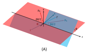
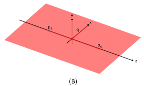
Figure 1: (A) The photon frame. The $x$ and $z$ axes have been aligned with the spatial components of $X^{\mu}$ and $Z^{\mu}$ from Eq. (3). The blue plane is the $e^{+}e^{-}$ plane. (B) The hadron frame, with the hadrons exactly back-to-back. See text for further explanation.

II.2 Hadron frame

In the hadron frame, $p_{A}$ and $p_{B}$ are back-to-back along the $z$ axis – see Fig. 1 (B). The measure of the deviation from the back-to-back configuration is then the size of the virtual photon’s transverse momentum, $q_{h\text{T}}$. In light-cone coordinates and neglecting masses the momenta in the hadron frame are:

$$q_{h} =\left(\sqrt{\frac{Q^{2}+q^{2}_{h\text{T}}}{2}},\sqrt{\frac{Q^{2}+q^{2}_{h\text{T}}}{2}},\bm{q}_{h\text{T}}\right)\,,$$ (4a)

$$p_{A,h} =(p_{A,h}^{+},0,\bm{0})\,,$$ (4b)

$$p_{B,h} =(0,p_{B,h}^{-},\bm{0})\,.$$ (4c)

We have chosen to boost along the $z$-axis in the hadron frame until $q_{h}^{+}$ = $q_{h}^{-}$. Useful Lorentz-invariant variables are

$$z_{A}=\frac{p_{A}\cdot{p}_{B}}{q\cdot{p}_{B}}=\frac{p_{A,h}^{+}}{q_{h}^{+}}\,,\qquad z_{B}=\frac{p_{A}\cdot{p}_{B}}{q\cdot{p}_{A}}=\frac{p_{B,h}^{-}}{q_{h}^{-}}\,.$$ (5)

Note that we take the Lorentz invariant ratios to define $z_{A}$ and $z_{B}$. Since in this paper we assume that the hadron masses are negligible, these are also equal to the light-cone ratios shown. For a treatment that includes kinematical mass effects, see Ref. Mulders and Van Hulse (2019). The transverse momentum of the photon in the hadron frame is:

$$q^{2}_{h\text{T}}=\frac{2\ p_{A}\cdot{q}\ p_{B}\cdot{q}}{p_{A}\cdot{p}_{B}}-Q^{2}=Q^{2}\tan^{2}\left(\delta\theta/2\right)\,.$$ (6)

As $\delta\theta$ approaches 180^∘ in Fig. 1, far from the back-to-back configuration, $q_{h\text{T}}$ as defined in Eq. (6) diverges, while for $\delta\theta\approx 0$ it approaches zero. From here forward, we will drop the $h$ subscript for simplicity and $q_{\text{T}}$ will be understood to refer to the hadron frame photon transverse momentum.

The transverse momentum has an absolute kinematical upper bound:

$${q_{\rm T}^{\rm Max}}^{2}\leq\frac{Q^{2}(1-z_{A})(1-z_{B})}{1-(1-z_{A})(1-z_{B})}\,.$$ (7)

Note that $q^{2}_{\text{T}}$ can be larger or smaller than $Q^{2}$ depending on $z_{A}$ and $z_{B}$. The invariant mass-squared of the dihadron pair is

$$\left(p_{A}+p_{B}\right)^{2}=z_{A}z_{B}\left(Q^{2}+q^{2}_{\text{T}}\right)\,,$$ (8)

which is of size $Q^{2}$ as long as $z_{A}$ and $z_{B}$ are fixed and not too small.

II.3 The transverse momentum differential cross section

Written in terms of a leptonic and a hadronic tensor, the cross section under consideration is

$$E_{A}E_{B}\frac{\mathrm{d}\sigma_{AB}}{\mathrm{d}^{3}\bm{p}_{A}{}\mathrm{d}^{3}\bm{p}_{B}{}}=\frac{\alpha_{\rm em}^{2}}{8\pi^{3}Q^{6}}L_{\mu\nu}W^{\mu\nu}$$ (9)

where the leptonic tensor is

$$L^{\mu\nu}\equiv l^{\mu}l^{\prime\nu}+l^{\prime\mu}l^{\nu}-g^{\mu\nu}l^{\prime}\cdot l\,,$$ (10)

and the hadronic tensor is

$$W^{\mu\nu}\equiv 4\pi^{3}\sum_{X}\langle 0|j^{\mu}(0)|p_{A},p_{B},X\rangle\langle p_{A},p_{B},X|j^{\nu}(0)|0\rangle\delta^{(4)}(q-p_{A}-p_{B}-p_{X})\,,$$ (11)

where $j$ is the electromagnetic current, $p_{X}$ is the momentum of the unobserved part of the final state, and the $\sum_{X}$ includes all sums and integrals over unobserved final states $X$. The structure functions are related to the hadronic tensor through the decomposition

$$W^{\mu\nu}(q,p_{A},p_{B})= \left(-g^{\mu\nu}+\frac{q^{\mu}{q}^{\nu}}{Q^{2}}-Z^{\mu}{Z}^{\nu}\right)W_{T}+Z^{\mu}{Z}^{\nu}{W}_{L}\,.$$ (12)

where $W_{T}$ and $W_{L}$ are the unpolarized structure functions. The $T$ and $L$ subscripts denote transverse and longitudinal polarizations respectively for the virtual photon. For our purposes, we may neglect polarization and azimuthally dependent structure functions Collins (2011). A convenient way to extract each structure function in Eq. (12) is to contract the hadronic tensor with associated extraction tensors, $P_{L}^{\mu\nu}$ and $P_{T}^{\mu\nu}$:

$$W_{T}=P_{T}^{\mu\nu}W_{\mu\nu}\,,\qquad W_{L}=P_{L}^{\mu\nu}W_{\mu\nu}\,,$$ (13)

where

$$P_{T}^{\mu\nu}=\frac{1}{3}\left(-g^{\mu\nu}-Z^{\mu}{Z}^{\nu}+X^{\mu}{X}^{\nu}\right)\,,\qquad P_{L}^{\mu\nu}=Z^{\mu}{Z}^{\nu}\,,$$ (14)

with the $Z^{\mu}$ and $X^{\mu}$ defined as in Eq. (3).

After changing variables to $z_{A}$, $z_{B}$, $q_{\text{T}}$ (see Appendix A for details),

$$\frac{\mathrm{d}\sigma_{AB}}{\mathrm{d}z_{A}\mathrm{d}z_{B}\mathrm{d}q_{\text{T}}\mathrm{d}\cos\theta\mathrm{d}\phi}=\frac{\alpha_{{\rm em}}^{2}z_{A}z_{B}\left(Q^{2}+q_{\text{T}}^{2}\right)^{2}q_{\text{T}}}{32\pi^{2}{Q}^{6}}\left[\left(1+\cos^{2}\theta\right)W_{T}+\sin^{2}\theta\ {W}_{L}\right]\,,$$ (15)

where $\theta$ and $\phi$ are the polar and azimuthal angles of lepton $l$ with respect to the $Z$ and $X$ directions in the photon frame. For the polarization independent case considered in this paper, we integrate this over $\theta$ and $\phi$ to get

$$\frac{\mathrm{d}\sigma_{AB}}{\mathrm{d}z_{A}\mathrm{d}z_{B}\mathrm{d}q_{\text{T}}}=\frac{\alpha_{{\rm em}}^{2}z_{A}z_{B}\left(Q^{2}+q_{\text{T}}^{2}\right)^{2}q_{\text{T}}}{12\pi{Q}^{6}}\left[2W_{T}+W_{L}\right].$$ (16)

In the small transverse momentum limit, the process in Eq. (1) is the one most simply and directly related to TMD ffs through derivations such as Ref. Collins and Soper (1981) or more recently in Ref. (Collins, 2011, Chapt. 13). Note that, apart from the dihadron pair, the final state is totally inclusive (with no specification of physical jets or properties like thrust). This and the measurement of transverse momentum relative to a $Z$-axis as defined as above is important for the derivation of factorization, at least in its most basic form, with standard TMD and collinear ffs as the relevant correlation functions. Measurements within a jet and relative to a thrust axis Seidl et al. (2019) of course contain important information in relation to TMD ffs, but the connection is less direct.

III Factorization at Large, Moderate and Small Transverse Momentum

To calculate in perturbative QCD, the differential cross section in Eq. (16) needs to be factorized into a hard part and ffs, and different types of factorization are appropriate depending on the particular kinematical regime. Assuming $z_{A,B}$ are large enough to ensure that hadrons originate from separately fragmenting quarks, the three kinematical regions of interest for semi-inclusive scattering are determined by the transverse momentum $q_{\text{T}}$. There are three major regions: i.) $q_{\text{T}}\sim Q$ so that $q_{\text{T}}$ and $Q$ are equally viable hard scales, ii.) $m\ll q_{\text{T}}\ll Q$ so that small $q_{\text{T}}$ approximations are useful but $q_{\text{T}}$ is large enough that intrinsic non-perturbative effects are negligible and logarithmic enhancements are only a small correction, iii.) $q_{\text{T}}\lesssim m$ and all aspects of a TMD-based treatment are needed, including non-perturbative intrinsic transverse momentum (see also Sec. IV). We will briefly summarize the calculation of each of these below.

III.1 The fixed $O\left(\alpha_{s}\right)$ cross section at large transverse momentum

The scenario under consideration is one in which the two observed hadrons are produced at wide angle (so that $(p_{A}+p_{B})^{2}\sim Q^{2}$), but are far from back-to-back (so that $q_{\text{T}}\sim Q$). This requires at least one extra gluon emission in the hard part. See Fig. 2 (A) for the general structure of Feynman graphs contributing at large $q_{\text{T}}$ and for our momentum labeling conventions.

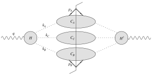
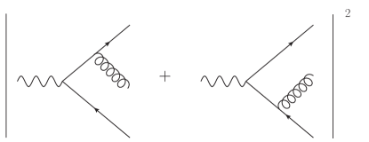
(a)	(b)

Figure 2: (a) The general diagrammatic structure contributing to Eq. (1) at large $q_{\text{T}}$ and at LO in $\alpha_{s}$. The outgoing partonic lines are dotted to indicate that generally they can be of any type. In the region of interest for this paper, their momenta deviate by wide angles from the back-to-back orientation for the dihadron pair. $H$ represents the hard part of the interaction and the $C_{A,B,C}$ are the collinear subgraphs Collins (2011). (b) The $O\left(\alpha_{s}\right)$ partonic contribution to the square-modulus amplitude in the factorization of (a).

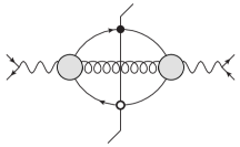
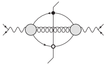
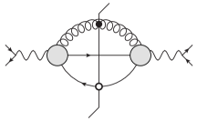
(A)	(B)	(C)
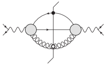
(D)	(E)	(F)

Figure 3: Partonic channels that contribute at order $\alpha_{s}$. Detailed explanation in Sec. III.1.

The basic statement of collinear factorization for the differential cross section is

$$E_{A}E_{B}\frac{\mathrm{d}\sigma_{AB}}{\mathrm{d}^{3}\bm{p}_{A}{}\mathrm{d}^{3}\bm{p}_{B}{}}=\sum_{i,j}\int_{z_{A}}^{1}\mathrm{d}\zeta_{A}\int_{z_{B}}^{1}\mathrm{d}\zeta_{B}\left(E_{A}E_{B}\frac{\mathrm{d}\hat{\sigma}_{ij}(\hat{z}_{A},\hat{z}_{B})}{\mathrm{d}^{3}\bm{p}_{A}{}\mathrm{d}^{3}\bm{p}_{B}{}}\right)d_{H_{A}/i}(\zeta_{A})d_{H_{B}/j}(\zeta_{B})\,$$ (17)

where the hat on the cross section in the integrand indicates that it is for the partonic subprocess $l_{1}+l_{2}\to k_{A}+k_{B}+X$. $k_{A}$ and $k_{B}$ will label the momenta of the partons that hadronize. The integrals are over the momentum fraction variables $\zeta_{A}$ and $\zeta_{B}$ that relate the hadron and parton momenta in Fig. 2:

$$k_{A}\equiv p_{A}/\zeta_{A}\,,\qquad k_{B}\equiv p_{B}/\zeta_{B}\,.$$ (18)

The $i,j$ sum is over the different possible flavors of parton that can hadronize, $i,j\in\{u,d,g,\bar{u}\dots\}$. The number of active flavors depends on the scale. The $d_{H_{A}/i}(\zeta_{A})$ and $d_{H_{B}/j}(\zeta_{B})$ are the fragmentation functions for flavor $i$($j$) partons to hadronize into hadrons of flavor $A$ ($B$). We use the standard abbreviations

$$\hat{z}_{A}=z_{A}/\zeta_{A}\,,\qquad\hat{z}_{B}=z_{B}/\zeta_{B}\,,$$ (19)

which follow from Eq. (18) and the partonic analogue of the definitions in Eq. (5). The momentum of the parton whose hadronization is unobserved is $k_{C}$ Collins et al. (2008); Accardi and Qiu (2008); Accardi and Signori (2019). After factorization, the hard part involves the square-modulus of the $H$ subgraph with massless, on-shell external partons. The graphs that contribute to this at lowest order are shown in Fig. 2(b).

It is useful to define a partonic version of the hadronic tensor,

$$\widehat{W}_{ij}^{\mu\nu}\equiv 4\pi^{3}\sum_{X}\langle 0|j_{ij}^{\mu}(0)|k_{A},k_{B},X\rangle\langle k_{A},k_{B},X|j_{ij}^{\nu}(0)|0\rangle\delta^{(4)}(q-k_{A}-k_{B}-p_{X})\,,$$ (20)

in which case

$$W^{\mu\nu}=\sum_{i,j}\int_{z_{A}}^{1}\frac{\mathrm{d}\zeta_{A}}{\zeta_{A}^{2}}\int_{z_{B}}^{1}\frac{\mathrm{d}\zeta_{B}}{\zeta_{B}^{2}}\widehat{W}_{ij}^{\mu\nu}(\hat{z}_{A},\hat{z}_{B})d_{H_{A}/i}(\zeta_{A})d_{H_{B}/j}(\zeta_{B})\,.$$ (21)

Working with the hadronic tensor and with the extraction tensors like Eq. (13) conveniently automates the steps to obtain any arbitrary structure function. The differential cross section is

$$\frac{\mathrm{d}\sigma_{AB}}{\mathrm{d}z_{A}\mathrm{d}z_{B}\mathrm{d}q_{\text{T}}}= \sum_{i,j}\int_{z_{A}}^{1}\frac{\mathrm{d}\zeta_{A}}{\zeta_{A}}\int_{z_{B}}^{1}\frac{\mathrm{d}\zeta_{B}}{\zeta_{B}}\left(\frac{\mathrm{d}\hat{\sigma}_{ij}(\hat{z}_{A},\hat{z}_{B})}{\mathrm{d}\hat{z}_{A}\mathrm{d}\hat{z}_{B}\mathrm{d}q_{\text{T}}}\right)d_{H_{A}/i}(\zeta_{A})d_{H_{B}/j}(\zeta_{B})\,,$$ (22)

and the partonic cross section can be expressed analogously to Eq. (16),

$$\frac{\mathrm{d}\hat{\sigma}_{ij}}{\mathrm{d}\hat{z}_{A}\mathrm{d}\hat{z}_{B}\mathrm{d}q_{\text{T}}}=\frac{\alpha_{\rm em}^{2}\hat{z}_{A}\hat{z}_{B}\left(Q^{2}+q_{\text{T}}^{2}\right)^{2}q_{\text{T}}}{12\pi{Q}^{6}}\left[2\widehat{W}_{T,ij}+\widehat{W}_{L,ij}\right]\,,$$ (23)

where $\widehat{W}_{T,ij}$ and $\widehat{W}_{L,ij}$ are partonic structure functions calculated from the graphs in Fig. 2(b).

Given the expressions for the squared amplitudes in Fig. 2(b), the evaluation of the differential cross section becomes straightforward. Each possible combination of final state parton pairs in Fig. 2(b) can hadronize into $H_{A}$ and $H_{B}$ with fragmentation functions that depend on both the fragmenting parton and final state hadron. Six such channels contribute at leading order in $\alpha_{s}$, and we organize these diagrammatically in Fig. 3, with $k_{A}$, $k_{B}$ and $k_{C}$ assigned to the quark, antiquark or gluon according to whether it hadronizes to $H_{A}$, $H_{B}$, or is unobserved. A solid dot marks the parton that hadronizes into $H_{A}$ (always $k_{A}$ parton momentum) and the open dot marks the parton that hadronizes into $H_{B}$ (always $k_{B}$ momentum). There is an integral over all momentum of the remaining line ($k_{C}$). Quark lines include all active quark flavors, and are shown separately from the anti-quark lines since they correspond to separate ffs. Notice that, unlike in the case of the $q_{T}$-integrated cross section for single hadron production, there is already sensitivity to the gluon fragmentation function at the lowest non-vanishing order. The analytic expressions needed for the calculation are summarized in Appendix B.

III.2 The asymptotic $\frac{q^{2}_{\text{T}}}{Q^{2}}\to 0$ limit

The small $q^{2}_{\text{T}}/Q^{2}$ limit of Eq. (22) involves considerable simplifications analogous to those obtained in TMD factorization, but applied to fixed order massless partonic graphs. It is potentially a useful simplification, therefore, in situations where $q^{2}_{\text{T}}$ is small enough that a $q^{2}_{\text{T}}/Q^{2}$ expansion applies, but still large enough that fixed order perturbative calculations are reasonable approximations. As we will see in later sections, it is also useful for estimating the borders of the regions where small $q^{2}_{\text{T}}/Q^{2}$ approximations are appropriate.

The asymptotic term is obtainable by directly expanding the fixed order calculation in powers of small $q_{\text{T}}/Q$, with a careful treatment of the soft gluon region in the integrals over $\zeta_{A}$ and $\zeta_{B}$. The steps are similar to those in SIDIS, and we refer to Ref. Nadolsky et al. (1999) for a useful discussion of them. When performed for the $e^{+}e^{-}$ annihilation case under consideration here, the result is

$$\frac{\mathrm{d}\sigma_{AB}^{ASY}}{\mathrm{d}z_{A}\mathrm{d}z_{B}\mathrm{d}q_{\text{T}}}=\frac{4\alpha_{\rm em}^{2}\alpha_{s}}{Q^{2}q_{\text{T}}}\sum_{q}e_{q}^{2} \left\{2C_{F}\left[\ln{\left(\frac{Q^{2}}{q^{2}_{\text{T}}}\right)}-\frac{3}{2}\right]\left(d_{H_{A}/q}(z_{A})d_{H_{B}/\bar{q}}(z_{B})+d_{H_{A}/\bar{q}}(z_{A})d_{H_{B}/q}(z_{B})\right)\right.$$

$$+d_{H_{A}/q}(z_{A})\left[(P_{\bar{q}\bar{q}}\otimes{d}_{H_{B}/\bar{q}})(z_{B})+(P_{g\bar{q}}\otimes{d}_{H_{B}/g})(z_{B})\right]\bigg{.}$$

$$+d_{H_{A}/\bar{q}}(z_{A})\left[(P_{qq}\otimes{d}_{H_{B}/q})(z_{B})+(P_{gq}\otimes{d}_{H_{B}/g})(z_{B})\right]\bigg{.}$$

$$+d_{H_{B}/q}(z_{B})\left[(P_{\bar{q}\bar{q}}\otimes{d}_{H_{A}/\bar{q}})(z_{A})+(P_{g\bar{q}}\otimes{d}_{H_{A}/g})(z_{A})\right]\bigg{.}$$

$$+d_{H_{B}/\bar{q}}(z_{B})\left[(P_{qq}\otimes{d}_{H_{A}/q})(z_{A})+(P_{gq}\otimes{d}_{H_{A}/g})(z_{A})\right]\bigg{\}}\,,$$ (24)

where $P_{ij}$ are the leading order unpolarized splitting functions

$$P_{qq}(z)=P_{\bar{q}\bar{q}}(z)=C_{F}\left[\frac{1+z^{2}}{\left(1-z\right)_{+}}+\frac{3}{2}\delta\left(1-z\right)\right]\,,\qquad P_{gq}(z)=P_{g\bar{q}}(z)=C_{F}\left[\frac{1+\left(1-z\right)^{2}}{z}\right]\,,$$ (25)

and $\otimes$ represents the convolution integral

$$(f\otimes{g})(z)=\int_{z}^{1}\frac{\mathrm{d}\zeta}{\zeta}f(z/\zeta)g(\zeta)\,.$$ (26)

The “$()_{+}$” in Eq. (25) denotes the usual plus-distribution. The “$\rm ASY$” superscript on Eq. (III.2) symbolizes the asymptotically small $q^{2}_{\text{T}}/Q^{2}$ limit for the cross section. The sum over $q$ is a sum over all active quark flavors.

III.3 TMD ffs and the small $q_{T}$ region

In the small transverse momentum limit of the cross section, the $W_{L}$ structure function becomes power suppressed. The cross section in Eq. (16) is simply

$$\frac{\mathrm{d}\sigma_{AB}}{\mathrm{d}z_{A}\mathrm{d}z_{B}\mathrm{d}q_{\text{T}}}=\frac{\alpha_{{\rm em}}^{2}z_{A}z_{B}q_{\text{T}}}{6\pi{Q}^{2}}W_{T}\,,$$ (27)

and the structure function $W_{T}$ (or hadronic tensor) factorizes in a well known way into TMD fragmentation functions

$$W_{T}=\frac{8\pi^{3}z_{A}z_{B}}{Q^{2}}\sum_{q}\widehat{W}_{T,q}\int\frac{\mathrm{d}^{2}\bm{b}_{\text{T}}{}}{(2\pi)^{2}}e^{-i\bm{b}_{\text{T}}{}\cdot\bm{q}_{\text{T}}{}}\left[\tilde{D}_{H_{A}/q}\tilde{D}_{H_{B}/\bar{q}}+\tilde{D}_{A/\bar{q}}\tilde{D}_{B/q}\right]\,,$$ (28)

where

$$\widehat{W}_{T,q}=6Q^{2}e_{q}^{2}\,.$$ (29)

The $\tilde{D}_{H/q}$ are the TMD fragmentation functions in transverse coordinate $\bm{b}_{T}$ space. After evolution, the TMD ff for a hadron $H$ from quark $q$ is

$$\tilde{D}_{H/q} (z,\bm{b}_{T};\mu,\zeta_{D})=\sum_{j}\int_{z}^{1}\frac{d\hat{z}}{\hat{z}^{3}}\tilde{C}_{j/q}(z/\hat{z},b_{*};\zeta_{D},\mu)d_{H/j}(\hat{z},\mu_{b})$$

$$\times\exp\left\{\ln\frac{\sqrt{\zeta_{D}}}{\mu_{b}}\tilde{K}(b_{*};\mu_{b})+\int_{\mu_{b}}^{\mu}\frac{d\mu^{\prime}}{\mu}\left[\gamma(\mu^{\prime};1)-\ln\frac{\sqrt{\zeta_{D}}}{\mu^{\prime}}\gamma_{K}(\mu^{\prime})\right]+g_{H/j}(z,b_{T})+\frac{1}{2}g_{K}(b_{T})\ln\frac{\zeta_{D}}{\zeta_{D,0}}\right\}$$ (30)

The $j$ index runs over all quark flavors and includes gluons, and the functions $d_{H/j}(z,\mu_{b})$ are ordinary collinear ffs which are convoluted with coefficient functions $C_{j/q}$ derived from the the small $b_{T}$ limit of the TMDs. All perturbative contributions, $C_{j/q}$, $\tilde{K}$, $\gamma$, and $\gamma_{K}$ are known by now to several orders in $\alpha_{s}$ Rogers (2015); Scimemi (2019).

However, non-perturbative functions also enter to parametrize the truly non-perturbative and intrinsic parts of the TMD functions. These are $g_{H/j}$, which is hadron and flavor dependent, and $g_{K}$, which is independent of the nature of hadrons and parton flavors and controls the non-perturbative contribution to the evolution. When combined in a cross section $\zeta_{D_{A}}\times\zeta_{D_{B}}=Q^{4}$. Some common parametrizations used for phenomenological fits are

$$g_{H/j}(z,b_{T}) =-\frac{1}{4z^{2}}\langle K^{2}_{H/j,\text{T}}\rangle b_{T}^{2}\,,$$ (31)

$$g_{K}(b_{T}) =-\frac{1}{2}g_{2}b_{T}^{2}\,.$$ (32)

Perturbative parts of calculations are usually regulated in the large $b_{T}$ region by using, for example, the $b_{*}$ prescription with:

$$b_{*}(b_{T})=\frac{b_{T}}{\sqrt{1+\left(b_{T}/b_{\rm max}\right)^{2}}},\hskip 28.45274pt\mu_{b}(b_{*})\propto\frac{1}{b_{*}}\,.$$ (33)

While there are many ways to regulate large $b_{T}$, and many alternative proposals for parametrizing the non-perturbative TMD inputs $\langle K^{2}_{H/j,\text{T}}\rangle$ and $g_{2}$, the above will be sufficient for the purpose of capturing general trends in the comparison of large and small transverse momentum calculations in Sec. V.

IV Transverse Momentum Hardness

The question of what constitutes large or small transverse momentum warrants special attention, so we now consider how the kinematical configuration of the third parton in graphs of the form of Fig. 2(a), not associated with a fragmentation function, affects the sequence of approximations needed to obtain various types of factorization. Generally, the propagator denominators in the hard blob $H$ can be classified into two types depending on whether $k_{C}$ attaches inside a far off-shell virtual loop or to an external leg. If it attaches inside a virtual loop, the power counting is

$$\frac{1}{2\ k_{C}\cdot k_{A,B}+O(Q^{2})}\,,$$ (34)

and for an external leg attachment (the off-shell propagators in Fig. 2(b), for example)

$$\frac{1}{2\ k_{C}\cdot k_{A,B}+O(m^{2})}\,.$$ (35)

The coefficients of the $O(Q^{2})$ and $O(m^{2})$ are numerical factors roughly of size $1$. Here the $m^{2}$ is a small mass scale comparable to $\Lambda_{\rm QCD}^{2}$ or a small hadron mass-squared. Possible $O\left(m^{2}\right)$ terms in the Eq. (34) denominator can always be neglected relative to $O\left(Q^{2}\right)$ and so have not been written explicitly.

The question that needs to be answered to justify collinear versus TMD factorization is whether the $2\ k_{C}\cdot k_{A,B}$ terms are also small enough to be dropped, or if they are large enough that they can be treated as hard scales comparable to $Q^{2}$, or if the true situation is somewhere in between. The fixed order calculations like those of the previous section is justified if

$$\left|\frac{2\ k_{C}\cdot k_{A,B}}{Q^{2}}\right|$$ (36)

is not much smaller than $1$. A quick estimate of the relationship between this ratio and $q^{2}_{\text{T}}/Q^{2}$ is obtained as follows:

$$\left|\frac{2\ k_{C}\cdot k_{A,B}}{Q^{2}}\right|\approx\left|\frac{(q-k_{B,A})^{2}}{Q^{2}}\right|\approx\left|\frac{(q-\frac{p_{B,A}}{z_{B,A}})^{2}}{Q^{2}}\right|=\frac{q^{2}_{\text{T}}}{Q^{2}}\,,$$ (37)

where the first “$\approx$” means momentum conservation is used with $k_{A,B,C}^{2}\approx 0$, and the second “$\approx$” means the standard small $q^{2}_{\text{T}}$ approximation for the photon vertex, $\zeta_{A}\approx z_{A}$, is being used. For the denominator in Eq. (35), the relevant ratio is $m^{2}/(2\ k_{C}\cdot k_{A,B})$, and arguments similar to the above give

$$\left|\frac{m^{2}}{2\ k_{C}\cdot k_{A,B}}\right|\approx\frac{m^{2}}{q^{2}_{\text{T}}}\,.$$ (38)

If Eq. (37) is $O\left(1\right)$ while Eq. (38) is much less than one, then the approximations on which collinear factorization at large $q^{2}_{\text{T}}$ is based are justified.

The situation is reversed if Eq. (38) is $O\left(1\right)$ or larger but Eq. (37) is small. In that case, the neglect of the $O\left(m^{2}\right)$ effects (including intrinsic transverse momentum) in the Eq. (35) denominators is unjustified. However, the smallness of Eq. (37) means neglecting the $2k_{C}\cdot k_{A,B}$ terms in the hard vertex is now valid, and this leads to its own set of extra simplifications. Ultimately, such approximations are analogous to those used in the derivation of TMD factorization.

An additional way to estimate the hardness of $q^{2}_{\text{T}}$ is to compare with the kinematical maximum in Eq. (7). For $z_{A,B}\gtrsim.4$, it can produce a significantly smaller ratio than Eq. (37). For example, for $z_{A,B}=.5$, $q_{\rm T}^{\rm Max}/Q^{2}=1/3$. Certainly, small $q^{2}_{\text{T}}/Q^{2}$ approximations fail near such thresholds.

The range of possible transverse momentum regions can be summarized with three categories:

• Intrinsic transverse momentum: Eq. (38) is of size $1$ or larger, but Eq. (37) is a small suppression factor. TMD factorization, or a similar approach that accounts for small transverse momentum effects, is needed. Such a kinematical regime is ideal to studying intrinsic transverse momentum properties of fragmentation functions.

• Hard transverse momentum: Eq. (38) is much less than $1$, and Eq. (37) is comparable to $1$. Therefore, fixed order calculations like those of the previous section are justified.

• Intermediate transverse momentum: Eq. (38) is much less than $1$, but Eq. (37) is also much less than one. In this case, the previous two types of approximations are simultaneously justifiable. Transverse momentum dependence is mostly perturbative, but large logarithms of $q^{2}_{\text{T}}/Q^{2}$ imply that transverse momentum resummation and/or TMD evolution are nevertheless important.

The large transverse momentum fixed order calculations are the most basic of these, since they involve only collinear factorization starting with tree level graphs, so it is worthwhile to confirm that there is a region where they are phenomenologically accurate, as is the aim of the present paper. Direct comparisons between fixed order calculations and measurements can help to confirm or challenge the above expectations. For example, consider a case where $Q\sim 10$ GeV while the largest measurable transverse momenta about $\sim 7$ GeV. Then logarithms of $q^{2}_{\text{T}}/Q^{2}$, i.e., $|\ln.7^{2}|\sim.7$, are not large while Eq. (37) is a non-negligible $\sim 0.5$. These are ideal kinematics, therefore, for testing the regime where fixed order calculations are expected to apply.

V Large and Small Transverse Momentum Comparison

We begin our comparison by computing the fixed order collinear factorization based cross section for the $q^{2}_{\text{T}}\sim Q^{2}$ region using the DSS14 ff parametrizations de Florian et al. (2015), and we compare with the calculation of the asymptotic term in Eq. (III.2). The results are shown for both moderate $Q\sim 12$ GeV and for large $Q\sim 50$ GeV in Fig. 4 (left panel), with $z_{A,B}=0.3$ in both cases. The horizontal axis is the ratio $q_{\text{T}}/q_{\rm T}^{\rm Max}$, using Eq. (7) to make the proximity to the kinematical large-$q^{2}_{\text{T}}$ threshold clearly visible.

The exact kinematical relation (for $1\to 3$ scattering) between $\zeta_{B}$ and $\zeta_{A}$ is

$$\zeta_{B}=z_{B}\frac{(Q^{2}+q^{2}_{\text{T}})(z_{A}-\zeta_{A})}{q^{2}_{\text{T}}z_{A}+Q^{2}(z_{A}-\zeta_{A})}\,,$$ (39)

while the cross section in the asymptotically small $q^{2}_{\text{T}}/Q^{2}$ limit has either $\zeta_{A}=z_{A}$ with $\zeta_{B}\geq z_{B}$ or $\zeta_{B}=z_{B}$ with $\zeta_{A}\geq z_{A}$. The asymptotic phase space in the $\zeta_{B}$-$\zeta_{A}$ plane approaches a rectangular wedge shape in the small $q^{2}_{\text{T}}$ limit, shown as the solid black lines in Fig. 4 (right panel) for fixed values of $z_{A}=z_{B}$. For comparison, the differently colored dashed, dot-dashed, and dotted lines show the $\zeta_{B}$-$\zeta_{A}$ curves from Eq. (39) for various nonzero $q^{2}_{\text{T}}$. The deviation between the colored and black curves gives one indication of the degree of error introduced by taking the small $q^{2}_{\text{T}}$ limit. Fig. 4(right panel) shows how these grow at large $z_{A,B}$. A non-trivial kinematical correlation forms between momentum fractions $\zeta_{A}$ and $\zeta_{B}$ in the large $z_{A},z_{B}$ and large $q^{2}_{\text{T}}$ regions. Notice also that the contours are scale independent, since $q_{\rm T}^{\rm Max}$ is proportional to $Q^{2}$, so kinematical errors from small $q_{\text{T}}$ approximations are likewise scale independent.

The point along the horizontal axis where the asymptotic term turns negative is another approximate indication of the region above which small $q^{2}_{\text{T}}/Q^{2}$ approximations begin to fail and the fixed order collinear factorization treatment should become more reliable, provided $z_{A,B}$ are at fixed moderate values and $q_{\rm T}$ is not too close to the overall kinematical thresholds. That point is shown in Fig. 4(left) for two representative values of small ($Q=12$ GeV) and large $Q=50$ GeV. The transition is at rather small transverse momentum, roughly $q_{\rm T}/q_{\rm T}^{\rm Max}\sim 0.2$, though the exact position depends on a number of details, including the shapes of the collinear fragmentation functions. If the asymptotic term is used as the indicator, then the transition is also roughly independent of $Q$.

We are ultimately interested in asking how the fixed order collinear calculation compares with existing TMD ff parametrizations near the small-to-large transverse momentum transition point. A reasonable range of non-perturbative parameters like $\langle K^{2}_{H/j,\text{T}}\rangle$ and $g_{2}$ in Eqs. (31)–(32), can be estimated from a survey of existing phenomenological fits. We will make the approximation that all light flavors have equal $\langle K^{2}_{H/j,\text{T}}\rangle=\langle K^{2}_{\text{T}}\rangle$ for pion production. Then values for $\langle K^{2}_{H/j,\text{T}}\rangle$ lie in the range from about $.11$ GeV^-2 to $.23$ GeV^-2 Bacchetta et al. (2017), which straddles the value $0.16$ GeV^-2 in Ref. Schweitzer et al. (2010). For $g_{2}$, we use a minimum value of $0$ to estimate the effect of having no non-perturbative evolution at all, and we use a maximum value of $.184$ GeV^-2, from Ref. Konychev and Nadolsky (2006), which is at the larger range of values that have been extracted. This range also straddles the $g_{2}=.13$ GeV^-2 found in Ref. Bacchetta et al. (2017). In all cases, we use the lowest order perturbative anomalous dimensions since these were used in most of the Gaussian-based fits above. Collectively, the numbers above produce the blue bands in Fig. 5 (left). The references quoted above generally include uncertainties for their parametrizations of $\langle K^{2}_{j,\text{T}}\rangle$ and $g_{2}$, but these are much smaller than the uncertainty represented by the blue band in Fig. 5 (left). We use a representative estimate of $b_{\rm max}=1.0$ GeV^-1; Refs. Bacchetta et al. (2017) and  Konychev and Nadolsky (2006) use slightly larger values ($1.123$ GeV^-1 and $1.5$ GeV^-1 respectively), but larger $b_{\rm max}\gtrsim 1.0$ GeV^-1 also has a small effect and only increases the general disagreement with the collinear fixed order calculation.

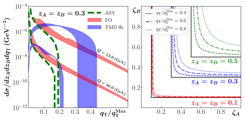
Figure 4: (left): LO collinear factorization predictions for the inclusive $e^{+}e^{-}$ to dihadron cross section (Sec. III and Appendix B), for $Q=12,50$ GeV. The red band shows the range covered by switching the renormalization group scale between $\mu=Q$ (lower edge) and $q_{\text{T}}$ (upper edge). The blue band is the calculation performed using TMD ffs, and the band shows the range covered by the values of the non-perturbative parameters discussed in Sec. V. (right): correlation between partonic momentum fractions $\zeta_{A,B}$ for various values of $q_{\rm T}/q_{\rm T}^{\rm Max}$.

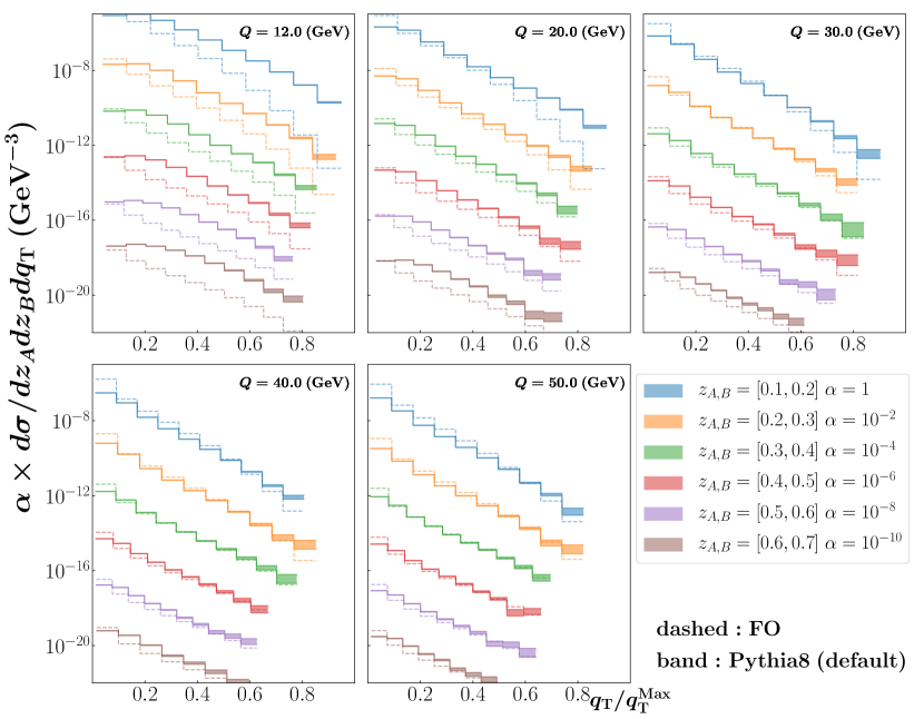
Figure 5: The lowest order collinear factorization calculation from Sec. III compared with $\pi^{+}/\pi^{-}$ pair production simulated by PYTHIA-8 with default settings for different ranges of $z_{A,B}$ and for increasing values of $Q$, starting with $Q=12$ GeV. Both the fixed-order calculation and the simulation are averaged in the $z_{A,B}$ bins. The uncertainty on the bands is purely statistical.

Observe in Fig. 4 (left) that, despite our somewhat overly liberal band sizes for the TMD ff calculation, large tension in the intermediate transverse momentum region between the TMD ff-based cross section and the fixed order collinear calculation nevertheless remains. For the $z_{A,B}\approx.3$ shown, $q_{\rm T}^{\rm Max}\approx Q$. The $Q=50$ GeV curves show that as $Q$ is raised, this tension diminishes, though at a perhaps surprisingly slow rate. For $Q=12$ GeV, the asymptotic and fixed order terms approach one another, but only at very small $q_{\text{T}}$. The curves contained within the blue band deviate qualitatively from the asymptotic and fixed order terms across all transverse momentum, and the blue band badly overshoots both in the intermediate region of $q_{\text{T}}\approx 2-3$ GeVs. The result is reminiscent of the situation with other processes – see, for example, Fig. 6 of Boglione et al. (2015a) for SIDIS.

Interestingly, data for the observable of Eq. (1) for $\pi^{+}/\pi^{-}$ production simulated with PYTHIA 8 Sjöstrand et al. (2006, 2015) using default settings, shows quite reasonable agreement with the collinear factorization calculation in the expected range of intermediate transverse momentum and $z_{A,B}$ and very large $Q$, validating the analytic fixed order collinear calculation in regions where it is most expected that the collinear calculations and the simulation should overlap. We illustrate this in Fig. 5, where for $z_{A,B}$ between $0.2$ and $0.6$ the fixed order analytic calculation agrees within roughly a factor of 2 with the PYTHIA-generated spectrum for $Q\gtrsim 20$ GeV and for $q_{\rm T}/q_{\rm T}^{\rm Max}\sim 0.5$. At smaller $Q\lesssim 20$ GeV, the agreement between the fixed order calculation and the simulation is much worse, though because $Q$ is relatively small and the event generator includes only the leading order hard scattering (with parton showering), it is unclear how the disagreement in that region should be interpreted. Nevertheless, it is interesting to observe that the trend wherein the collinear factorization calculation undershoots data, seen in SIDIS Gonzalez-Hernandez et al. (2018) and Drell-Yan Bacchetta et al. (2019b) calculations, seems to persist even here. In the future, it would be interesting to perform a more detailed Monte Carlo study that incorporates treatments of higher order hard scattering.

VI Conclusions

As one of the simplest processes with non-trivial transverse momentum dependence, dihadron production in $e^{+}e^{-}$ annihilation is ideal for testing theoretical treatments of transverse momentum distributions generally. A goal of this paper has been to spotlight its possible use as a probe of the transition between kinematical regions corresponding to different types of QCD factorization. There have been a number of studies highlighting tension between large transverse momentum collinear factorization based calculation and cross section measurements for Drell-Yan and SIDIS, Refs. Daleo et al. (2005); Kniehl et al. (2005); Gonzalez-Hernandez et al. (2018); Wang et al. (2019); Bacchetta et al. (2019b). Whether the resolution lies with a need for higher orders, a need to refit correlation functions, large power-law corrections in the region of moderate $Q$ Liu and Qiu (2019), or still other factors that are not yet understood remains unclear.

An important early step toward clarifying the issues is an examination of trends in standard methods of calculation in the large transverse momentum region. Motivated by this, we have examined the simplest LO calculation relevant for large deviation from the back-to-back region in detail. Agreement with Monte Carlo-generated distributions at large $Q$ supports the general validity of such calculations. However, when comparing the result in the intermediate transverse momentum region with expectations obtained from TMD fragmentation functions, we find trends reminiscent of those discussed above for SIDIS and Drell-Yan scattering at lower $Q$. Namely, the collinear factorization calculation appears to be overly suppressed. We view this as significant motivation to study the intermediate transverse momentum region both experimentally and theoretically. An advantage in the $e^{+}e^{-}$ annihilation is the larger value of $Q$ relative to processes like semi-inclusive deep inelastic scattering.

While we have focused on the large transverse momentum limit, the observations above are relevant to other kinematical regions such as small transverse momentum, as well as to polarization dependent observables, and their physical interpretation, since the detailed shape of the transverse momentum distributions for any region depend on the transitions to other regions.

It is important to note that order $\alpha_{s}^{2}$ corrections can be quite large Daleo et al. (2005); Kniehl et al. (2005); Gonzalez-Hernandez et al. (2018); Wang et al. (2019), and we plan to address these in future studies, though generally higher order effects have not been sufficient in other processes to eliminate tension. Keeping this in mind, it is worthwhile nevertheless to speculate on other possible resolutions. One is that the hard scale $Q$ might be too low for a simplistic division of transverse momentum into regions such as discussed in Sec. IV. It is true that as $Q$ gets smaller, the separation between large and small transverse momentum becomes squeezed, and it is possible that the standard methods for treating the transition between separately well defined regions is inapplicable. As a hard scale, however, $Q\sim 12$ GeV is well above energies that are normally understood to be near to the lower limits of applicability of standard perturbation theory methods (typical scales for SIDIS measurements are around $Q\sim 2$ GeV, for example). Another possibility is that fragmentation functions in the large $\zeta$ range probed at large $q_{\text{T}}$ are not sufficiently constrained. An important next step is to determine whether the description of large transverse momentum processes generally can be improved via a simultaneous analysis of multiple processes at moderate $Q$ with simple and well- established collinear factorization treatments. We plan to investigate this in future work.

Appendix A Variables Changes

The left hand side of Eq. (9) can be rewritten as

$$\frac{\left|\bm{p}_{A}\right|}{\left|\bm{p}_{B}\right|}\frac{\mathrm{d}\sigma_{AB}}{\mathrm{d}\left|\bm{p}_{B}\right|\mathrm{d}\Omega_{B}\mathrm{d}^{3}\bm{p}_{A}}$$ (40)

Change of variables is easiest in a center of mass frame where $p_{B}$ is on the z-axis. In this frame, the hadron momenta in terms of $Q$, $q_{\text{T}}$, $z_{A}$, and $z_{B}$ (in Cartesian coordinates) are:

$$p_{A} =\left(\frac{z_{A}}{2Q}\left(Q^{2}+q^{2}_{\text{T}}\right),-z_{A}\bm{q}_{\text{T}},-\frac{z_{A}}{2Q}\left(Q^{2}-q^{2}_{\text{T}}\right)\right)$$ (41)

$$p_{B} =\left(\frac{z_{B}}{2Q}\left(Q^{2}+q^{2}_{\text{T}}\right),\bm{0}_{\text{T}}{},\frac{z_{B}}{2Q}\left(Q^{2}+q^{2}_{\text{T}}\right)\right).$$ (42)

and the lepton momentum $l$ is:

$$l=\left(\frac{Q}{2},\frac{Q}{2}\sin\theta\cos\phi,\frac{Q}{2}\sin\theta\sin\phi,\frac{Q}{2}\cos\theta\right).$$ (43)

Therefore:

$$\left|\bm{p}_{A}\right| =\frac{z_{A}}{2Q}\left(Q^{2}+q^{2}_{\text{T}}\right)$$

$$\left|\bm{p}_{B}\right| =\frac{z_{B}}{2Q}\left(Q^{2}+q^{2}_{\text{T}}\right)$$

$$\mathrm{d}^{3}\bm{p}_{A}\mathrm{d}\left|\bm{p}_{B}\right| =\frac{q_{\text{T}}(Q^{2}+q_{\text{T}}^{2})^{2}z_{A}^{2}}{4Q^{2}}\mathrm{d}z_{A}\mathrm{d}z_{B}\mathrm{d}q_{\text{T}}\mathrm{d}\phi_{A}$$

$$\mathrm{d}\Omega_{B} =\mathrm{d}\cos\theta\mathrm{d}\phi$$ (44)

After integrating over $\phi_{A}$, Eq. (9) then becomes:

$$\frac{\mathrm{d}\sigma_{AB}}{\mathrm{d}z_{A}\mathrm{d}z_{B}\mathrm{d}q_{\text{T}}\mathrm{d}\cos\theta\mathrm{d}\phi}=\frac{\alpha_{{\rm em}}^{2}z_{A}z_{B}\left(Q^{2}+q_{\text{T}}^{2}\right)^{2}q_{\text{T}}}{16\pi^{2}{Q}^{8}}L_{\mu\nu}W^{\mu\nu}.$$ (45)

Appendix B Fixed Order Expressions

The partonic structure functions $\widehat{W}_{T,ij}$ and $\widehat{W}_{L,ij}$ can be obtained by contracting the extraction tensors (Eq. (14)) with the partonic tensor $\widehat{W}^{\mu\nu}$. The relation between the partonic tensor and the squared amplitude of the hard part is:

$$\widehat{W}^{\mu\nu}_{ij}=4\pi^{3}\int\frac{\mathrm{d}^{3}\bm{k}_{C}}{2k_{C}^{0}(2\pi)^{3}}\delta^{(4)}\left(q-k_{A}-k_{B}-k_{C}\right)|\mathcal{\widehat{M}}|^{2,\mu\nu}_{ij}=\frac{1}{2}\delta_{+}(k_{C}^{2})|\mathcal{\widehat{M}}|^{2,\mu\nu}_{ij}\,.$$ (46)

The resulting partonic cross sections are

$$\frac{\mathrm{d}\hat{\sigma}_{q\bar{q}}}{\mathrm{d}\hat{z}_{A}\mathrm{d}\hat{z}_{B}\mathrm{d}q_{\text{T}}}=\frac{\mathrm{d}\hat{\sigma}_{\bar{q}q}}{\mathrm{d}\hat{z}_{A}\mathrm{d}\hat{z}_{B}\mathrm{d}q_{\text{T}}}= \frac{8\alpha_{\rm em}^{2}\alpha_{s}e_{q}^{2}\hat{z}_{A}\hat{z}_{B}\delta\left(k_{C}^{2}\right)q_{\text{T}}\left(Q^{2}+q^{2}_{\text{T}}\right)^{3}\left(6Q^{2}+5q^{2}_{\text{T}}\right)\left(\hat{z}_{A}^{2}+\hat{z}_{B}^{2}\right)}{9Q^{6}\left(Q^{2}(\hat{z}_{A}-1)+q^{2}_{\text{T}}\hat{z}_{A}\right)\left(Q^{2}(\hat{z}_{B}-1)+q^{2}_{\text{T}}\hat{z}_{B}\right)}$$ (47a)

$$\frac{\mathrm{d}\hat{\sigma}_{qg}}{\mathrm{d}\hat{z}_{A}\mathrm{d}\hat{z}_{B}\mathrm{d}q_{\text{T}}}=\frac{\mathrm{d}\hat{\sigma}_{\bar{q}g}}{\mathrm{d}\hat{z}_{A}\mathrm{d}\hat{z}_{B}\mathrm{d}q_{\text{T}}}= -8\alpha_{\rm em}^{2}\alpha_{s}e_{q}^{2}\hat{z}_{A}\hat{z}_{B}\delta\left(k_{C}^{2}\right)q_{\text{T}}\left(Q^{2}+q^{2}_{\text{T}}\right)^{2}\left[2Q^{4}\left(14+3\hat{z}_{B}^{2}-14\hat{z}_{B}+2\hat{z}_{A}\left(3\hat{z}_{A}+4\hat{z}_{B}-7\right)\right)\right.$$

$$\left.+5q_{\text{T}}^{4}\left(\hat{z}_{B}^{2}+2\hat{z}_{B}\hat{z}_{A}+2\hat{z}_{A}^{2}\right)+Q^{2}q^{2}_{\text{T}}\left(11\hat{z}_{B}^{2}-28\hat{z}_{B}+2\hat{z}_{A}\left(11\hat{z}_{A}+13\hat{z}_{B}-14\right)\right)\right]$$

$$\Bigg{/}\left(9Q^{6}\left(Q^{2}({\hat{z}}_{A}-1)+q^{2}_{\text{T}}{\hat{z}}_{A}\right)\left(Q^{2}(\hat{z}_{B}+{\hat{z}}_{A}-1)+q^{2}_{\text{T}}(\hat{z}_{B}+{\hat{z}}_{A})\right)\right)$$ (47b)

$$\frac{\mathrm{d}\hat{\sigma}_{gq}}{\mathrm{d}\hat{z}_{A}\mathrm{d}\hat{z}_{B}\mathrm{d}q_{\text{T}}}=\frac{\mathrm{d}\hat{\sigma}_{g\bar{q}}}{\mathrm{d}\hat{z}_{A}\mathrm{d}\hat{z}_{B}\mathrm{d}q_{\text{T}}}= -8\alpha_{\rm em}^{2}\alpha_{s}e_{q}^{2}\hat{z}_{A}\hat{z}_{B}\delta\left(k_{C}^{2}\right)q_{\text{T}}\left(Q^{2}+q^{2}_{\text{T}}\right)^{2}\left[2Q^{4}\left(14+3\hat{z}_{A}^{2}-14\hat{z}_{A}+2\hat{z}_{B}\left(3\hat{z}_{B}+4\hat{z}_{A}-7\right)\right)\right.$$

$$\left.+5q_{\text{T}}^{4}\left(\hat{z}_{A}^{2}+2\hat{z}_{A}\hat{z}_{B}+2\hat{z}_{B}^{2}\right)+Q^{2}q^{2}_{\text{T}}\left(11\hat{z}_{A}^{2}-28\hat{z}_{A}+2\hat{z}_{B}\left(11\hat{z}_{B}+13\hat{z}_{A}-14\right)\right)\right]$$

$$\Bigg{/}\left(9Q^{6}\left(Q^{2}({\hat{z}}_{B}-1)+q^{2}_{\text{T}}{\hat{z}}_{B}\right)\left(Q^{2}(\hat{z}_{A}+{\hat{z}}_{B}-1)+q^{2}_{\text{T}}(\hat{z}_{A}+{\hat{z}}_{B})\right)\right)$$ (47c)