BNB autoregressions for modeling integer-valued time series with extreme observations

Abstract

This article introduces a general class of heavy-tailed autoregressions for modeling integer-valued time series with outliers. The proposed specification is based on a heavy-tailed mixture of negative binomial distributions that features an observation-driven dynamic equation for the conditional expectation. The existence of a unique stationary and ergodic solution for the class of autoregressive processes is shown under a general contraction condition. The estimation of the model can be easily performed by Maximum Likelihood given the closed form of the likelihood function. The strong consistency and the asymptotic normality of the estimator are formally derived. Two examples of specifications illustrate the flexibility of the approach and the relevance of the theoretical results. In particular, a linear dynamic equation and a score-driven equation for the conditional expectation are considered. The score-driven specification is shown to be particularly appealing as it delivers a robust filtering method that attenuates the impact of outliers. An empirical application to the time series of narcotics trafficking reports in Sydney illustrates the effectiveness of the method in handling extreme observations.

Key words: heavy-tailed distributions, integer-valued time series, observation-driven models, robust filtering.

1 Introduction

Time series data with integer-valued observations are often encountered in empirical applications. Classical continuous-response models, such as autoregressive moving average (ARMA) models, are not suited for the modeling of such series. Over the last few decades, researchers have developed methods that can properly account for the discreteness of the data. A standard approach is to consider observation-driven models that feature time variation in the intensity parameter of the Poisson distribution (Fokianos et al.,, 2009; Ferland et al.,, 2006; Davis et al.,, 2003). A limitation of the Poisson distribution is that it imposes equidispersion, i.e. mean equal to the variance. Equidispersion is typically restrictive in empirical applications and therefore overdispersed distributions, such as the negative binomial, are often considered (Davis and Wu,, 2009; Zhu,, 2011). Other extensions considered in the literature include multivariate integer-valued models and the use of zero-inflated distributions, which are suited for time series with large numbers of zeros. We refer the reader to Davis et al., (2016) for an overview of recent developments.

Extreme observations, or outliers, are often present when analyzing time series data. The study of time series with outliers has a long history that dates back to Fox, (1972). Ignoring extreme observations in the dataset leads to statistical models that offer a poor description of the series of interest. Additionally, statistical inference can also be problematic in the presence of outilers. There is a vast literature on modeling continuous-valued time series with extreme observations. Models are typically embedded with heavy-tailed distributions that are capable of describing outliers as tail events. The Student’s t-distribution is often used for this purpose and robust specifications for the dynamic component of the model are employed to attenuate the impact of outliers (Creal et al.,, 2011; Harvey and Luati,, 2014). On the other hand, to the best of our knowledge, the current literature lacks modeling methods for time series of integer-valued data when outliers are present.

In this article, we introduce a general class of observation-driven models for integer-valued time series data with extreme observations. The approach is based on a heavy-tailed mixture of negative binomial distributions, known as the beta negative binomial (BNB) distribution. The class of models features a dynamic location parameter and a BNB conditional distribution, which describes extreme observations as tail events. We derive conditions for stationarity, ergodicity and finiteness of moments for the proposed class of stochastic processes. Additionally, we show that inference can be easily performed by Maximum Likelihood (ML), given that the likelihood function is available in closed form. The strong consistency and the asymptotic normality of the ML estimator are proved under general conditions. We consider and study two different specifications of the dynamic component of the model. The first is a simple linear autoregression for the conditional mean. Instead, the second is based on the Generalized Autoregressive Score (GAS) framework of Creal et al., (2013) and Harvey, (2013). This second specification delivers a robust filter that attenuates the impact of extreme observations on the conditional expectation of the BNB process. Finally, we present an empirical analysis to the time series of police reports of narcotics trafficking in Sydney, Australia. The results illustrate the capability of the proposed approach in modeling time series data with extreme observations.

The paper is structured as follows. Section 2 provides a brief review of the BNB distribution. Section 3 introduces the class of BNB autoregressive processes and discusses their stochastic properties. Section 4 derives the asymptotic properties of the ML estimator. Section 5 introduces the linear specification of the model and discusses its properties. Section 6 introduces the score-driven specification. Section 7 presents the empirical application. Section 8 concludes.

2 Preliminaries

We start by reviewing some properties of the BNB distribution, which will be useful in the rest of the paper. The BNB distribution arises as a beta mixture of negative binomial distributions. In particular, let $Y$ conditional on $P$ have a negative binomial distribution, $Y|P\sim\mathcal{NB}(r,P)$, with dispersion parameter $r$ and success probability $P$. Assume further that $P$ has a beta distribution, $P\sim\mathcal{B}eta(\alpha,\beta)$, with shape parameters $\alpha$ and $\beta$. Then, the marginal distribution of $Y$ is BNB with the following probability mass function (pmf)

$$\mathbb{P}(Y=y)=\frac{\Gamma(y+r)}{\Gamma(y+1)\Gamma(r)}\frac{B(\alpha+r,\beta+y)}{B(\alpha,\beta)},\quad\text{for}\quad y\in\mathbb{N},$$

where $\Gamma(\cdot)$ denotes the gamma function and $B(\cdot,\cdot)$ the beta function. The parameter $\alpha$ is the tail parameter of the BNB, which determines the heaviness of the right tail. The smaller $\alpha$ the heavier the tail. Throughout the paper, we parametrize the BNB distribution in terms of its mean. More specifically, we consider $\beta=(\alpha-1)\lambda/r$. In this way, the parameter $\lambda$ represents the mean of the BNB distribution when the mean is finite, which is the case when $\alpha>1$. We say that $Y\sim\mathcal{BNB}(\lambda,r,\alpha)$ has a BNB distribution with mean $\lambda>0$, dispersion parameter $r>0$ and tail parameter $\alpha>1$ if

$$\mathbb{P}(Y=y)=\frac{\Gamma(y+r)}{\Gamma(y+1)\Gamma(r)}\frac{B\Big{(}\alpha+r,(\alpha-1)\lambda/r+y\Big{)}}{B\Big{(}\alpha,(\alpha-1)\lambda/r\Big{)}},\quad y\in\mathbb{N}.$$ (1)

The BNB distribution enables us to account for extreme observations, which can be seen as tail events. Furthermore, we note that the BNB can approximate arbitrarily well the negative binomial distribution as well as the Poisson distribution. As the tail parameter diverges, $\alpha\rightarrow\infty$, the BNB distribution $\mathcal{BNB}(\lambda,r,\alpha)$ converges to a negative binomial distribution with dispersion parameter $r$ and success probability $\lambda/(r+\lambda)$. Further, as the dispersion parameter diverges, $r\rightarrow\infty$, the BNB converges to a Poisson distribution with mean $\lambda$. For a more detailed review of the BNB distribution, we refer the reader to Wang, (2011).

3 BNB autoregressive models

Consider a time series of counts $\{y_{t}\}_{t\in\mathbb{Z}}$ with the following conditional distribution

$$y_{t}|\mathcal{F}_{t-1}\sim\mathcal{BNB}(\lambda_{t},r,\alpha),\quad t\in\mathbb{Z},$$ (2)

where $r>0$, $\alpha>1$, and $\mathcal{F}_{t}$ denotes the $\sigma$-field generated by $\{y_{t},y_{t-1}\dots\}$. The conditional mean process $\lambda_{t}=\mathbb{E}(y_{t}|\mathcal{F}_{t-1})$ is specified by the following stochastic recurrence equation (SRE)

$$\lambda_{t+1}=g_{\boldsymbol{\theta}}(y_{t},\lambda_{t}),\quad t\in\mathbb{Z},$$ (3)

where $g_{\boldsymbol{\theta}}(\cdot,\cdot)$ is a parametric updating function that maps from $\mathbb{N}\times\mathbb{R}^{+}$ into $\mathbb{R}^{+}$, and $\boldsymbol{\theta}\in\mathbb{R}^{n}$ is a parameter vector. We denote by $\boldsymbol{\kappa}\in\mathbb{R}^{n+2}$ the entire parameter vector of the model $\boldsymbol{\kappa}=(\boldsymbol{\xi}^{\top},\boldsymbol{\theta}^{\top})^{\top}$, where $\boldsymbol{\xi}=(r,\alpha)^{\top}$. Note that in the above formulation, for simplicity of exposition, $\lambda_{t}$ is assumed to be $\mathcal{F}_{t-1}$-measurable. Below, we show that under a contraction condition on $g_{\boldsymbol{\theta}}$ the model’s equations admit a unique stationary and ergodic causal solution and $\lambda_{t}$ is $\mathcal{F}_{t-1}$-measurable.

The BNB autoregressive model specified in (2) and (3) can describe extreme observations in time series data by means of the heavy-tailed BNB conditional pmf. A small value of the tail parameter $\alpha$ indicates that extreme observations are more likely to occur. The $m$-th conditional moment of the BNB autoregressive process $\mathbb{E}(y_{t}^{m}|\mathcal{F}_{t-1})$ is finite if and only if $\alpha>m$. However, as we shall discuss below, finiteness of unconditional moments requires further conditions on the updating function $g_{\boldsymbol{\theta}}$. In Sections 5 and 6, two examples of specifications of the updating function are presented. We shall see that a robust updating function may be desirable to reduce the impact of outliers on the conditional mean $\lambda_{t}$.

In the rest of the section, we study the stochastic properties of the BNB autoregression described by equations (2) and (3). We derive conditions on the updating function $g_{\boldsymbol{\theta}}$ that ensure the process to be strictly stationary and ergodic and that guarantee the existence of the first two unconditional moments of $y_{t}$. The first result that we obtain is the stationarity and ergodicity of the process and existence of the first moment under a contraction condition. The proof of the result is based on the approach of Doukhan and Wintenberger, (2008) for weakly dependent chains with infinite memory. We highlight that this type of contraction condition is widely used in the literature of integer-valued processes, see , for instance, Davis and Liu, (2016) for an application to exponential families. We also obtain that the contraction condition ensures that $\lambda_{t}$ is $\mathcal{F}_{t-1}$-measurable.

Theorem 3.1 (stationarity and ergodicity).

Consider the BNB autoregressive process given by Equations (2) and (3). Furthermore, assume that the following contraction condition holds

$$|g_{\boldsymbol{\theta}}(y,\lambda)-g_{\boldsymbol{\theta}}(y^{*},\lambda^{*})|\leq c_{1}|y-y^{*}|+c_{2}|\lambda-\lambda^{*}|,$$ (4)

where $c_{1}$ and $c_{2}$ are some positive constants such that $c_{1}+c_{2}<1$. Then, the following results hold true:
(i) There exists a unique strictly stationary and ergodic causal solution $\{(y_{t},\lambda_{t})\}_{t\in\mathbb{Z}}$ with a finite first moment $\mathbb{E}(y_{t})<\infty$.
(ii) There exists a measurable function $g_{\boldsymbol{\theta}}^{\infty}$ such that $\lambda_{t}=g_{\boldsymbol{\theta}}^{\infty}(y_{t-1},y_{t-2},\dots)$, i.e. $\lambda_{t}$ is $\mathcal{F}_{t-1}$-measurable.

Theorem 3.1 requires the sum of the Lipschitz coefficients $c_{1}$ and $c_{2}$ to be smaller than one to ensure stationarity, ergodicity and finiteness of the first unconditional moment of $y_{t}$. However, a stricter contraction is needed to obtain the finiteness of the second moment. The next result imposes sufficient conditions on $c_{1}$ and $c_{2}$ to obtain $\mathbb{E}(y_{t}^{2})<\infty$, and hence the weak stationarity of the BNB autoregressive process.

Theorem 3.2 (weak stationarity).

Assume that $\alpha>2$ and that the contraction condition in (4) holds with

$$\frac{(r+1)(\alpha-1)}{r(\alpha-2)}c_{1}^{2}+c_{2}^{2}+2c_{1}c_{2}<1.$$

Then $y_{t}$ has a finite second moment $\mathbb{E}(y_{t}^{2})<\infty$. Hence $\{y_{t}\}_{t\in\mathbb{Z}}$ is weakly stationary.

We note that, besides a stricter contraction condition, Theorem 3.2 also requires the tail parameter $\alpha$ to be greater than two. This is needed because the conditional second moment of $y_{t}$ is finite if only if $\alpha>2$.

The results in Theorems 3.1 and 3.2 are of key importance to derive the asymptotic properties of the ML estimator. In particular, as we shall see in Section 4, the strict stationarity condition in Theorem 3.1 is sufficient for the consistency of the ML estimator. Instead, the additional conditions in Theorem 3.2 are needed for the asymptotic normality to hold. In Sections 5 and 6, Theorems 3.1 and 3.2 will be employed to establish the stochastic properties of a linear and a score-driven BNB autoregression.

4 Maximum Likelihood estimation

In this section, we discuss the estimation of the BNB autoregression by ML. We derive conditions to ensure consistency and asymptotic normality of the ML estimator. We assume that a subset of a realized path from the BNB autoregressive process in (2) and (3) with true parameter value $\boldsymbol{\kappa}=\boldsymbol{\kappa}_{0}$ is observed $\{y_{t}\}_{t=1}^{T}$. Here $T$ denotes the sample size. The likelihood function is available in closed form through a prediction error decomposition. In particular, the average log-likelihood function is

$$\hat{L}_{T}({\boldsymbol{\kappa}})=\frac{1}{T}\sum_{t=1}^{T}\hat{l}_{t}({\boldsymbol{\kappa}})=\frac{1}{T}\sum_{t=1}^{T}\log p(y_{t}|\hat{\lambda}_{t}({\boldsymbol{\theta}}),r,\alpha),$$

where $p$ denotes the conditional pmf, given by

$$p(y_{t}|\hat{\lambda}_{t}({\boldsymbol{\theta}}),r,\alpha)=\frac{\Gamma(y_{t}+r)}{\Gamma(y_{t}+1)\Gamma(r)}\frac{B\Big{(}\alpha+r,(\alpha-1)\hat{\lambda}_{t}({\boldsymbol{\theta}})/r+y_{t}\Big{)}}{B\Big{(}\alpha,(\alpha-1)\hat{\lambda}_{t}({\boldsymbol{\theta}})/r\Big{)}}.$$

The filtered time-varying parameter $\hat{\lambda}_{t}({\boldsymbol{\theta}})$ is obtained recursively using the observed data $\{y_{t}\}_{t=1}^{T}$

$$\hat{\lambda}_{t+1}({\boldsymbol{\theta}})=g_{\boldsymbol{\theta}}(y_{t},\hat{\lambda}_{t}({\boldsymbol{\theta}})),$$ (5)

where the recursion is initialized at a fixed point $\hat{\lambda}_{1}({\boldsymbol{\theta}})\in\mathbb{R}^{+}$. We note that initializing the recursion in (5) is needed since the observed data starts from time $t=1$. This is quite standard in the literature of observation-driven models. Finally, the ML estimator $\hat{\boldsymbol{\kappa}}_{T}$ is defined as the maximizer of the likelihood function

$$\hat{\boldsymbol{\kappa}}_{T}=\operatorname*{arg\,sup}_{{\boldsymbol{\kappa}}\in{K}}\hat{L}_{T}({\boldsymbol{\kappa}}),$$ (6)

where $K=\Xi\times\Theta$ with $\Xi\subset(0,\infty)\times(2,\infty)$ and $\Theta\subset\mathbb{R}^{n}$ being compact parameter sets.

4.1 Consistency

In order to establish the consistency of the ML estimator, we first derive the stochastic limit properties of the filtered parameter $\hat{\lambda}_{t}$ defined in (5). Note that $\hat{\lambda}_{t}(\cdot)$ is a stochastic function that maps from $\Theta$ into $\mathbb{R}^{+}$. The stability of the filtered parameter $\hat{\lambda}_{t}$ is often referred in the literature as invertibility (Straumann and Mikosch,, 2006; Blasques et al.,, 2018). Because of the initialization, $\hat{\lambda}_{t}$ evaluated at the true parameter value, $\hat{\lambda}_{t}(\boldsymbol{\theta}_{0})$, does not correspond to the true conditional mean $\lambda_{t}$. In the following, we show that $\{\hat{\lambda}_{t}\}_{t\in\mathbb{N}}$ converges exponentially a.s. (e.a.s.) and uniformly in $\Theta$ to a stationary and ergodic sequence of functions $\{\tilde{\lambda}_{t}\}_{t\in\mathbb{N}}$ such that $\tilde{\lambda}_{t}(\boldsymbol{\theta}_{0})=\lambda_{t}$ with probability one. We start by imposing a continuity condition on the updating function $g_{\boldsymbol{\theta}}$, which ensures that $\boldsymbol{\theta}\mapsto\hat{\lambda}_{t}({\boldsymbol{\theta}})$ is continuous in $\Theta$ with probability one.

Assumption 4.1.

The function $({\boldsymbol{\theta}},\lambda)\mapsto g_{\boldsymbol{\theta}}(y,\lambda)$ is continuous in $\Theta\times\mathbb{R}^{+}$ for any $y\in\mathbb{N}$.

Next, we assume that the contraction condition holds for all $\boldsymbol{\theta}$ in the parameter set $\Theta$, which contains the true parameter value $\boldsymbol{\theta}_{0}$. We note that this assumption is not restrictive since, in general, $\Theta$ can be defined as a compact ball around the true parameter vector $\boldsymbol{\theta}_{0}$.

Assumption 4.2.

The contraction condition in (4) is satisfied for any ${\boldsymbol{\theta}}\in\Theta$. Furthermore $\boldsymbol{\theta}_{0}\in\Theta$.

The next result ensures the uniform convergence over $\Theta$ of the filtered parameter $\hat{\lambda}_{t}({\boldsymbol{\theta}})$ to a stationary and ergodic limit $\tilde{\lambda}_{t}({\boldsymbol{\theta}})$. Here $\|\cdot\|_{\Theta}$ denotes the supremum norm. Given a function $f:\Theta\mapsto\mathbb{R}$, the supremum norm is $\|f\|_{\Theta}=\sup_{\boldsymbol{\theta}\in\Theta}|f(\boldsymbol{\theta})|$.

Proposition 4.1 (invertibility).

Let Assumptions 4.1 and 4.2 hold, then the filter $\{\hat{\lambda}_{t}({\boldsymbol{\theta}})\}_{t\in\mathbb{N}}$ converses e.a.s. and uniformly over $\Theta$ to a unique stationary and ergodic sequence $\{\tilde{\lambda}_{t}({\boldsymbol{\theta}})\}_{t\in\mathbb{Z}}$,

$$\|\hat{\lambda}_{t}-\tilde{\lambda}_{t}\|_{\Theta}\xrightarrow{e.a.s.}0,\quad t\rightarrow\infty,$$

for any initialization $\hat{\lambda}_{1}({\boldsymbol{\theta}})\in\mathbb{R}^{+}$. Furthermore, $\tilde{\lambda}_{t}$ has a bounded moment uniformly over $\Theta$, $\mathbb{E}\|\tilde{\lambda}_{t}\|_{\Theta}<\infty$.

Proposition 4.1 plays a crucial role to ensure that the likelihood function $\hat{l}_{t}(\boldsymbol{\tau})$, which depends on the approximate filter $\hat{\lambda}_{t}$, converges to a stationary and ergodic limit $l_{t}(\boldsymbol{\tau})=p(y_{t}|\tilde{\lambda}_{t}({\boldsymbol{\theta}}),r,\alpha)$, which depends on limit filter $\tilde{\lambda}_{t}$. In this way, $l_{t}(\boldsymbol{\tau}_{0})$ corresponds to the true conditional log-pmf of the BNB autoregressive model.

Next, building on the invertibility result, we impose some additional conditions to obtain the strong consistency of the ML estimator. The next assumption imposes a lower bound on the updating function.

Assumption 4.3 (lower bound).

There is a constant $\bar{c}>0$ such that $g_{\boldsymbol{\theta}}(y,\lambda)\geq\bar{c}$ for any $({\boldsymbol{\theta}},y,\lambda)\in\Theta\times\mathbb{N}\times\mathbb{R}^{+}$.

Finally, we impose an identifiability condition on the parametric updating function $g_{{\boldsymbol{\theta}}}$. This condition is needed to ensure that different parameter values of ${\boldsymbol{\theta}}$ give observationally different paths of $\tilde{\lambda}_{t}({\boldsymbol{\theta}})$.

Assumption 4.4 (identifiability).

For any ${\boldsymbol{\theta}}_{1},{\boldsymbol{\theta}}_{2}\in\Theta$ and $\lambda\in\mathbb{R}^{+}$, the equality $g_{{\boldsymbol{\theta}}_{1}}(y,\lambda)=g_{{\boldsymbol{\theta}}_{2}}(y,\lambda)$ holds true for all $y\in\mathbb{N}$ if and only if ${\boldsymbol{\theta}}_{1}={\boldsymbol{\theta}}_{2}$.

Under these conditions, we obtain the strong consistency of the ML estimator.

Theorem 4.1 (consistency).

Let Assumptions 4.1-4.4 hold and let ${\boldsymbol{\kappa}}_{0}\in K$, then the ML estimator defined in (6) is strongly consistent, that is,

$$\hat{\boldsymbol{\kappa}}_{T}\xrightarrow{a.s.}{\boldsymbol{\kappa}}_{0},\quad\text{as}\quad T\rightarrow\infty.$$

4.2 Asymptotic normality

We now focus on deriving the asymptotic normality of the ML estimator. First, we require the data generating process to have a finite second moment. A finite second moment is needed to ensure the existence of some moments for the derivatives of the log-likelihood, which are used to apply a central limit theorem to the score of the log-likelihood function.

Assumption 4.5 (weak stationarity).

The assumptions of Theorem 3.2 are satisfied for $\boldsymbol{\kappa}=\boldsymbol{\kappa}_{0}$.

The next assumption is needed to ensure that the Fisher information matrix is positive definite.

Assumption 4.6 (positive definite Fisher information).

The random variables of the vector $\frac{\partial g_{\boldsymbol{\theta}}}{\partial{\boldsymbol{\theta}}}(y_{t},\lambda_{t})|_{{\boldsymbol{\theta}}={\boldsymbol{\theta}}_{0}}$ are linearly independent.

Finally, the next assumption requires some regularity conditions on the updating function $g_{\boldsymbol{\theta}}$. In particular, we impose the updating function to be twice continuously differentiable and have some of its derivatives bounded by some linear functions of their arguments. Note that $\|\cdot\|$ denotes the $L_{1}$-norm when applied to a vector and the operator norm induced by the $L_{1}$-norm when applied to a matrix. Furthermore, we consider the following shorthand notation for the derivatives of the updating function: $g_{\boldsymbol{\theta}}^{d}(y,\lambda)=\partial g_{\boldsymbol{\theta}}(y,\lambda)/\partial d$. If $d$ is a 2-dimensional vector, then $g_{\boldsymbol{\theta}}^{d}(y,\lambda)$ denotes the second order partial derivative with respect to the elements of the vector. For instance, if $d=(\boldsymbol{\theta},\boldsymbol{\theta})$, then $g_{\boldsymbol{\theta}}^{\boldsymbol{\theta}\boldsymbol{\theta}}(y,\lambda)=\partial^{2}g_{\boldsymbol{\theta}}(y,\lambda)/\partial\boldsymbol{\theta}\partial\boldsymbol{\theta}^{\top}$.

Assumption 4.7.

The function $(\boldsymbol{\theta},\lambda)\mapsto g_{\boldsymbol{\theta}}(y,\lambda)$ is twice continuously differentiable with respect to both $\boldsymbol{\theta}$ and $\lambda$. Furthermore, for any ${\boldsymbol{\theta}}\in\Theta$

$$\|g_{\boldsymbol{\theta}}^{d}(y,\lambda)-g_{\boldsymbol{\theta}}^{d}(y^{*},\lambda^{*})\|\leq b_{1}|y-y^{*}|+b_{2}|\lambda-\lambda^{*}|,$$

for $d\in\{\lambda,{\boldsymbol{\theta}},(\lambda,\lambda),({\boldsymbol{\theta}},\lambda),({\boldsymbol{\theta}},{\boldsymbol{\theta}})\}$ and some positive constants $b_{1}$ and $b_{2}$.

The next result delivers the asymptotic normality of the ML estimator.

Theorem 4.2 (asymptotic normality).

Let Assumptions 4.1-4.7 hold and ${\boldsymbol{\kappa}}_{0}\in\text{int}(K)$, then the ML estimator defined in (6) has the following asymptotic distribution

$$\sqrt{T}(\hat{\boldsymbol{\kappa}}_{T}-{\boldsymbol{\kappa}}_{0})\xrightarrow{d}N(\boldsymbol{0},{\boldsymbol{\text{F}}}_{0}^{-1}),\quad\text{as}\quad T\rightarrow\infty,$$

where ${{\boldsymbol{\text{F}}}}_{0}=-\mathbb{E}\left[\frac{\partial^{2}l_{t}(\boldsymbol{\kappa}_{0})}{\partial{\boldsymbol{\kappa}}\partial{\boldsymbol{\kappa}}^{\top}}\right]$.

In practice, the Fisher information matrix ${\boldsymbol{\text{F}}}_{0}$ needs to be estimated. A consistent estimator is obtained by plugging in the ML estimator into the second derivative of the log-likelihood

$$\hat{\boldsymbol{\text{F}}}_{T}=-\frac{1}{T}\sum_{t=1}^{T}\frac{\partial^{2}\hat{l}_{t}(\hat{\boldsymbol{\kappa}}_{T})}{\partial{\boldsymbol{\kappa}}\partial{\boldsymbol{\kappa}}^{\top}}.$$

The next result shows that the estimator given above delivers a strongly consistent estimate for the asymptotic covariance matrix of the ML estimator.

Proposition 4.2.

Let the assumptions of Theorem 4.2 hold, then the estimator of the asymptotic covariance matrix is strongly consistent, that is,

$${\hat{\boldsymbol{\text{F}}}^{-1}}_{T}\xrightarrow{a.s.}{\boldsymbol{\text{F}}}_{0}^{-1},\quad\text{as}\quad T\rightarrow\infty.$$

5 BNB-INGARCH model

5.1 The model

An intuitive and simple way to specify the conditional mean $\lambda_{t}$ is to consider a linear autoregressive process driven by past observations. Count processes with a linear specification of the conditional mean are often referred in the literature as integer-valued generalized autoregressive conditional heteroscedastic (INGARCH) models (Ferland et al.,, 2006). We define the BNB-INGARCH model through the following equations

$$y_{t}|\mathcal{F}_{t-1}\sim\mathcal{BNB}(\lambda_{t},r,\alpha),\quad\lambda_{t+1}=\omega+\phi\lambda_{t}+\tau y_{t},$$ (7)

where $\omega>0$, $\phi\geq 0$ and $\tau>0$ are static parameters to be estimated. These parameters are restricted to be positive to guarantee that $\lambda_{t}$ is strictly positive with probability one. A linear autoregressive specification for the conditional expectation $\lambda_{t}$ is often considered for Poisson and negative binomial autoregressions, see Ferland et al., (2006), Fokianos et al., (2009) and Zhu, (2011). We refer to these models as the Po-INGARCH and NB-INGARCH models, respectively. We can immediately see that the BNB-INGARCH model can approximate arbitrarily well both the Po-INGARCH and the NB-INGARCH model since the BNB distribution converges to the negative binomial as $\alpha\rightarrow\infty$ and to the Poisson as, additionally, $r\rightarrow\infty$.

The next result relies on Theorem 3.1 and 3.2 to derive conditions for strict and weak stationarity of the BNB-INGARCH process.

Theorem 5.1.

Let the BNB-INGARCH process in (7) satisfy

$$\tau+\phi<1.$$ (8)

Then, the process admits a strictly stationary and ergodic solution with a finite first moment $\mathbb{E}(y_{t})<\infty$. Additionally, let $\alpha>2$ and

$$\frac{(r+1)(\alpha-1)}{r(\alpha-2)}\tau^{2}+\phi^{2}+2\tau\phi<1.$$ (9)

Then, the stationary solution has a finite second moment $\mathbb{E}(y_{t}^{2})<\infty$. Hence, it is weakly stationary.

Finally, we derive the strong consistency and asymptotic normality of the ML estimator of the BNB-INGARCH model by appealing to Theorem 4.1 and 4.2.

Theorem 5.2.

Let the observed series $\{y_{t}\}_{t=1}^{T}$ be generated by the BNB-INGARCH process in (7) with parameter value $\boldsymbol{\kappa}_{0}=(r_{0},\alpha_{0},\omega_{0},\phi_{0},\tau_{0})^{\top}$. Furthermore, let $\boldsymbol{\kappa}_{0}\in K$ where, $K$ is compact parameter set such that $\phi+\tau<1$ and $\omega>0$ for any $\boldsymbol{\kappa}\in K$. Then, the ML estimator defined in (6) is strongly consistent

$$\hat{\boldsymbol{\kappa}}_{T}\xrightarrow{a.s.}{\boldsymbol{\kappa}}_{0},\quad\text{as}\quad T\rightarrow\infty.$$

Assume further that $\boldsymbol{\kappa}_{0}$ satisfies the contraction condition in (9), $\alpha_{0}>2$, and $\boldsymbol{\kappa}_{0}\in int(K)$. Then, the ML estimator is asymptotically normally distributed

$$\sqrt{T}(\hat{\boldsymbol{\kappa}}_{T}-{\boldsymbol{\kappa}}_{0})\xrightarrow{d}N(\boldsymbol{0},{\boldsymbol{\text{F}}}_{0}^{-1}),\quad\text{as}\quad T\rightarrow\infty,$$

where ${{\boldsymbol{\text{F}}}}_{0}=-\mathbb{E}\left[\frac{\partial^{2}l_{t}(\boldsymbol{\kappa}_{0})}{\partial{\boldsymbol{\kappa}}\partial{\boldsymbol{\kappa}}^{\top}}\right]$.

The proof of Theorem 5.2, which is given in the Appendix, is obtained by checking that Assumptions 4.1-4.7 are satisfied. The small sample properties of the ML estimator are studied in a Monte Carlo experiment in the next section.

5.2 Monte Carlo simulation study

We investigate the small-sample properties of the ML estimator by means of a Monte Carlo simulation experiment. We generate samples of different sizes from the BNB-INGARCH model in (7) for several parameter values. The parameters are then estimated by ML. Table 1 reports the results of the experiment. The parameters $r$ and $\alpha$ are reparameterized in terms of their inverse. This is done because, especially in small samples, a given realized path from the BNB-INGARCH process may not present outliers and the estimate of $\alpha$ may become arbitrarily large since the likelihood function is flat for large $\alpha$.

Table 1: Simulation results for the ML estimator obtained from 1,000 Monte Carlo replications. The mean, the standard deviation (SD) and the root mean square error (RMSE) are reported for different parameter values and sample sizes. The parameter $\delta$ represents the unconditional mean of $y_{t}$, i.e. $\delta=\omega/(1-\phi-\tau)$.

		$\delta$	$\phi$	$\tau$	$r^{-1}$	$\alpha^{-1}$		$\delta$	$\phi$	$\tau$	$r^{-1}$	$\alpha^{-1}$
True value		10.00	0.50	0.20	0.10	0.20		10.00	0.68	0.20	0.10	0.20
$T=250$	Mean	9.965	0.457	0.198	0.125	0.172		9.991	0.648	0.197	0.116	0.167
	SD	0.984	0.191	0.065	0.091	0.052		1.607	0.120	0.059	0.093	0.052
	RMSE	0.985	0.196	0.065	0.094	0.059		1.607	0.124	0.059	0.094	0.062
$T=500$	Mean	9.960	0.476	0.199	0.124	0.183		9.984	0.664	0.199	0.114	0.182
	SD	0.689	0.135	0.046	0.079	0.037		1.192	0.071	0.040	0.073	0.037
	RMSE	0.690	0.137	0.046	0.082	0.040		1.192	0.073	0.040	0.075	0.041
$T=1000$	Mean	9.976	0.492	0.199	0.118	0.190		9.997	0.672	0.199	0.113	0.190
	SD	0.509	0.091	0.033	0.065	0.026		0.853	0.048	0.029	0.062	0.026
	RMSE	0.510	0.091	0.033	0.067	0.027		0.853	0.048	0.029	0.063	0.028
$T=2000$	Mean	9.982	0.497	0.199	0.113	0.194		10.013	0.677	0.199	0.108	0.196
	SD	0.363	0.060	0.023	0.053	0.019		0.592	0.033	0.020	0.044	0.019
	RMSE	0.364	0.060	0.023	0.055	0.020		0.592	0.033	0.020	0.044	0.019
True value		10.00	0.50	0.20	0.10	0.10		10.00	0.68	0.20	0.10	0.10
$T=250$	Mean	9.986	0.449	0.198	0.108	0.072		10.042	0.647	0.197	0.112	0.073
	SD	0.744	0.193	0.066	0.079	0.033		1.170	0.119	0.056	0.083	0.033
	RMSE	0.744	0.199	0.066	0.080	0.043		1.171	0.123	0.056	0.084	0.043
$T=500$	Mean	9.971	0.474	0.198	0.107	0.081		9.963	0.665	0.197	0.107	0.081
	SD	0.533	0.134	0.046	0.066	0.024		0.821	0.071	0.040	0.069	0.024
	RMSE	0.534	0.137	0.046	0.067	0.031		0.822	0.073	0.040	0.069	0.031
$T=1000$	Mean	9.994	0.490	0.198	0.107	0.087		10.012	0.673	0.198	0.108	0.088
	SD	0.384	0.093	0.031	0.057	0.017		0.608	0.049	0.027	0.056	0.017
	RMSE	0.384	0.093	0.031	0.057	0.021		0.608	0.050	0.027	0.057	0.021
$T=2000$	Mean	9.999	0.497	0.199	0.105	0.092		9.994	0.676	0.199	0.105	0.093
	SD	0.271	0.065	0.023	0.046	0.012		0.434	0.035	0.020	0.043	0.011
	RMSE	0.271	0.065	0.023	0.046	0.015		0.434	0.035	0.020	0.043	0.013

The results show that the estimates of all parameters seem to be consistent since the RMSE decreases as the sample size increases. Furthermore, we note that the estimation bias for $\delta$, $\delta=\omega/(1-\phi-\tau)$, and $\tau$ is negligible even for the smallest sample size considered in the experiment ($T=250$). This can be noted from the fact that the standard deviation is equivalent to the RMSE. On the other hand, the results show the presence of a small-sample bias in the estimates of $\phi$, $r$ and $\alpha$. In particular, the parameters $\phi$ and $r$ tend to be underestimated and $\alpha$ tends to be overestimated. However, the bias of all these estimates becomes negligible for larger sample sizes ($T=1,000$ and $T=2,000$). Finally, we note that the results seem to be coherent across the different parameter values. This is true even when $\phi=0.68$, which represents scenarios where the parameters are close to the boundary of the weak stationarity region given in (9).

6 A score-driven BNB autoregression

The BNB-INGARCH model presented in Section 5 accounts for extreme observations by means of the heavy tail of the conditional BNB distribution. However, the SRE for $\lambda_{t}$ is not robust against outliers: an extreme value of $y_{t}$ can have an arbitrary large impact on $\lambda_{t+1}$. In practice, it is often desirable to have a robust SRE that attenuates the impact of extreme observations on $\lambda_{t}$. We propose a robust specification that is based on the GAS framework of Creal et al., (2013) and Harvey, (2013). The conditional mean $\lambda_{t}$ is specified as an autoregressive process with innovation given by the score of the predictive likelihood. Score-driven models are widely used in the literature to specify robust updating functions in models with heavy-tailed distributions (Harvey and Luati,, 2014; Opschoor et al.,, 2017).

The BNB autoregression with a score-driven SRE, which we label as the BNB-GAS, is specified by the following equations

$$y_{t}|\mathcal{F}_{t-1}\sim\mathcal{BNB}(\lambda_{t},r,\alpha),\quad\log\lambda_{t+1}=\omega+\phi\log\lambda_{t}+\tau s_{t},$$ (10)

where $\omega\in\mathbb{R}$, $\phi\geq 0$ and $\tau>0$. The score innovation $s_{t}=\partial\log p(y_{t}|\lambda_{t},r,\alpha)/\partial\log\lambda_{t}$ is given by

$$s_{t}=\gamma\lambda_{t}\Big{(}\psi(\gamma\lambda_{t}+y_{t})+\psi(\gamma\lambda_{t}+\alpha)-\psi(\gamma\lambda_{t}+y_{t}+\alpha+r)-\psi(\gamma\lambda_{t})\Big{)},$$ (11)

where $\gamma=(\alpha-1)/r$ and $\psi(\cdot)$ denotes the digamma function, i.e. $\psi(x)=\partial\log\Gamma(x)/\partial x$. The exponential link function in (10) is considered to ensure that $\lambda_{t}$ is strictly positive with probability one. We refer to the score $s_{t}$ as the innovation of the process since $\mathbb{E}(s_{t}|\mathcal{F}_{t-1})=0$ with probability one.

The peculiarity of the BNB-GAS model is that the functional form of the score innovation reduces the impact of outliers. Figure 1 illustrates the sensitivity of $s_{t}$ to $y_{t}$ for different values of the tail parameter $\alpha$. We can see that the effect of large values of $y_{t}$ on $s_{t}$ is attenuated and the degree of attenuation depends on the tail parameter $\alpha$. The smaller the parameter $\alpha$ the more robust the score innovation $s_{t}$. This behavior of $s_{t}$ is quite intuitive since a small $\alpha$ introduces heavy tails in the conditional pmf of $y_{t}$ and therefore it generates outliers in the observed time series, see also Harvey and Luati, (2014) for a similar interpretation in the context of Student’s t-distributions. Furthermore, as it is shown in the proof of Theorem 6.1 in the Appendix, the score innovation is bounded by a constant $|s_{t}|\leq(\alpha+r+1)$. Therefore, $s_{t}$ is robust since it does not go to infinity as $y_{t}\rightarrow\infty$.

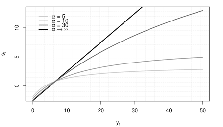
Figure 1: Impact of $y_{t}$ on the score innovation $s_{t}$ for different values of the tail parameter $\alpha$.

The BNB-GAS can approximate arbitrarily well some existing models that have been proposed in the literature. As $\alpha\rightarrow\infty$, the BNB-GAS becomes a score-driven model with negative binomial distribution, see Gorgi, (2018) for an application of the GAS framework with negative binomials. As additionally $r\rightarrow\infty$, the model becomes a Poisson autoregressive model, which belongs to the class of models introduced by Davis et al., (2003).

We now focus on the stochastic properties of the BNB-GAS. The next theorem gives sufficient conditions for the existence of a stationary and ergodic solution for the BNB-GAS process.

Theorem 6.1.

Consider the BNB-GAS process given in (10) and (11) and let $0\leq\phi<1$ and

$$\left(\tau\frac{\gamma(3\alpha+2r+3)+(\alpha+r+1)}{\gamma}+\phi\right)\exp\big{(}\tau(2\alpha+r+2)\big{)}<1.$$ (12)

Then, the process admits a stationary and ergodic solution with finite first moment $\mathbb{E}(y_{t})<\infty$.

The proof of this theorem is obtained by an application of Theorem 3.1. We note that the parameter restriction in (12) is a sufficient condition that makes the contraction condition of Theorem 3.1 hold. Given the complex functional form of $s_{t}$, it is not straightforward to obtain sharper upper bounds for the Lipschitz coefficients $c_{1}$ and $c_{2}$ in (4). The condition imposed on the parameters by (12) may be restrictive in practice, however, this condition highlights that the stationarity region is not degenerate.

Remark 6.1.

Under the conditions of Theorem 3.1, the BNB-GAS process admits a stationary and ergodic solution with $\mathbb{E}(y_{t}^{m})<\infty$ if and only if $\alpha>m$. This result holds true because $\lambda_{t}$ takes vales on a compact set with probability one, see the proof of Theorem 3.1 in the Appendix. This means that $\mathbb{E}(\lambda_{t}^{m})<\infty$ for any $m\in\mathbb{N}$. Therefore $\mathbb{E}(y_{t}^{m})<\infty$ if and only if $\mathbb{E}(y_{t}^{m}|\mathcal{F}_{t-1})<\infty$ with probability one, namely, $\alpha>m$.

7 Empirical application

In this section, we present an empirical application to the monthly number of police reports on narcotics trafficking in Sydney, Australia. The time series is from January 1995 to December 2016 and it is available in the New South Wales dataset of police reports. Figure 2 displays the plot and the empirical autocorrelation functions of the series. We can see that the dataset presents some extreme observations. In particular, the number of narcotics trafficking reports is exceptionally high in August 2000, March 2008 and May 2015. Therefore, BNB autoregressive models seem particularly suited to describe the autocorrelation structure and account for the outliers in the dataset.

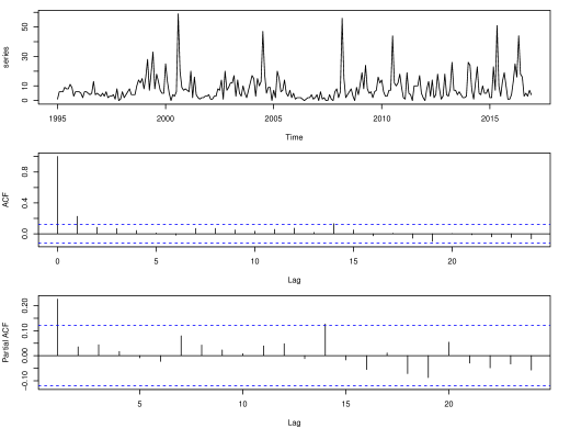
Figure 2: The first plot shows the monthly number of police reports for narcotics trafficking in Sydney. The second and third plots present the sample autocorrelation functions of the series.

Besides the BNB-INGARCH and the BNB-GAS, we consider two negative binomial specifications: one with a linear updating function and one based on the GAS framework, which we label as linear NB-INGARCH and NB-GAS respectively. As discussed before, these two models are limit cases, $\alpha\rightarrow\infty$, of the BNB-INGARCH and the BNB-GAS model. Table 2 reports the estimation results. The BNB specifications give a better description of the time series since they have lower values of the Akaike information criterion (AIC). More specifically, the BNB-GAS is the model that best fits the data. This suggests that the robust updating function given by the score innovation is beneficial in this case. Furthermore, the relevance of the BNB distribution can also be elicited from the relatively low estimates of the tail parameter $\alpha$, which is estimated to be around $5$ with a standard error of about $0.8$ for both BNB specifications. This further indicates that the extreme observations in the data are not properly described by a negative binomial distribution.

Table 2: Maximum Likelihood estimates of the models. Standard errors are in brackets. The last two columns contain the log-likelihood and the AIC, respectively. The parameter $\delta$ is $\delta=\omega/(1-\phi-\tau)$ for the INGARCH models and $\delta=\omega/(1-\phi)$ for the GAS models.

	$\delta$	$\phi$	$\tau$	$r$	$\alpha$	log-lik	AIC
BNB-INGARCH	8.549	0.481	0.267	6.521	4.819	-807.66	1625.33
	(1.104)	(0.223)	(0.085)	(3.394)	(0.744)
BNB-GAS	2.087	0.714	0.197	4.408	5.029	-807.04	1624.09
	(0.107)	(0.169)	(0.056)	(1.923)	(0.849)
NB-INGARCH	8.675	0.307	0.308	1.561	-	-821.22	1650.45
	(0.907)	(0.254)	(0.099)	(0.159)
NB-GAS	2.102	0.699	0.140	1.540	-	-822.59	1653.19
	(0.087)	(0.232)	(0.051)	(0.156)

Figure 3 reports the estimated conditional mean for the NB-GAS and the BNB-GAS. We can see that the BNB-GAS estimate of $\lambda_{t}$ is robust to the outliers in August 2000, March 2008 and May 2015. Instead, on the contrary, the estimate from the negative binomial specification is strongly affected by the outliers. This further highlights the empirical relevance of BNB autoregressive models in modeling integer-valued time series with extreme values.

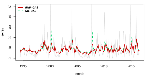
Figure 3: Estimated conditional mean $\lambda_{t}$ from the BNB-GAS model (in red) and the NB-GAS (in green). The original time series is displayed in gray.

8 Conclusion

This article introduces a general framework for modeling integer-valued time series with outliers. The paper proposes a class of observation-driven models that are based on a mixture of negative binomial distributions, known as the BNB distribution. The stochastic properties of the models and the asymptotic theory of ML estimation are formally discussed. Two different specifications are considered and studied. An empirical application illustrates the practical relevance of the approach. Further research may focus on extending the proposed method to more flexible specifications. For instance, relevant developments may include embedding the model with a zero-inflated BNB distribution to handle time series with large numbers of zeros.

Appendix A Appendix

A.1 Proofs

Proof of Theorem 3.1.

First we show that (i) holds true. For convenience, we rewrite the equations of the BNB autoregressive process as follows

$$y_{t}=F_{\lambda_{t}}^{-1}(u_{t}),\quad\lambda_{t+1}=g_{{\boldsymbol{\theta}}}(F_{\lambda_{t}}^{-1}(u_{t}),\lambda_{t}),$$

where $\{u_{t}\}_{t\in\mathbb{Z}}$ is an iid sequence of uniform random variables, $u_{t}\sim\mathcal{U}(0,1)$, and $F_{\lambda_{t}}^{-1}(u)=\inf_{z\in\mathbb{R}}\{u\leq F_{\lambda_{t}}(z)\}$, $u\in(0,1)$, where $F_{\lambda_{t}}(z)$, $z\in\mathbb{R}$, is the cumulative distribution function of a BNB random variable $\mathcal{BNB}(\lambda_{t},r,\alpha)$. We prove the result by showing that there is a unique stationary and ergodic causal solution $\{\lambda_{t}\}_{t\in\mathbb{Z}}$ with $\mathbb{E}(\lambda_{t})<\infty$ by an application of Theorem 3.1 in Doukhan and Wintenberger, (2008) (see also Remark 3.1). Then it is immediate to conclude that there is a unique stationary and ergodic causal solution $\{(y_{t},\lambda_{t})\}_{t\in\mathbb{Z}}$ and, given $\alpha>1$, we have $\mathbb{E}(y_{t})<\infty$. In the following, we show that the conditions (3.1) and (3.2) of Theorem 3.1 in Doukhan and Wintenberger, (2008) are satisfied. Note that (3.3) trivially holds given $\alpha>1$. From the contraction condition in (4), we obtain that

$$\mathbb{E}\left|g_{\boldsymbol{\theta}}\left(F_{x_{1}}^{-1}(u_{0}),x_{1}\right)-g_{\boldsymbol{\theta}}\left(F_{x_{2}}^{-1}(u_{0}),x_{2}\right)\right| =\int_{0}^{1}\left|g_{\boldsymbol{\theta}}\left(F_{x_{1}}^{-1}(u),x_{1}\right)-g_{\boldsymbol{\theta}}\left(F_{x_{2}}^{-1}(u),x_{2}\right)\right|du$$

$$\leq c_{1}\left|x_{1}-x_{2}\right|+c_{2}\int_{0}^{1}\left|F_{x_{1}}^{-1}(u)-F_{x_{2}}^{-1}(u)\right|du.$$

Now, if $x_{1}\geq x_{2}$, by appealing to the stochastic ordering result in Lemma A.7, we obtain that $F_{x_{1}}^{-1}(u)\geq F_{x_{2}}^{-1}(u)$ for any $u\in(0,1)$. Therefore, we have that

$$\mathbb{E}\left|g_{\boldsymbol{\theta}}\left(F_{x_{1}}^{-1}(u_{0}),x_{1}\right)-g_{\boldsymbol{\theta}}\left(F_{x_{2}}^{-1}(u_{0}),x_{2}\right)\right| \leq c_{1}\left|x_{1}-x_{2}\right|+c_{2}\int_{0}^{1}\left|F_{x_{1}}^{-1}(u)-F_{x_{2}}^{-1}(u)\right|du$$

$$=c_{1}\left|x_{1}-x_{2}\right|+c_{2}\left(\int_{0}^{1}F_{x_{1}}^{-1}(u)du-\int_{0}^{1}F_{x_{2}}^{-1}(u)du\right)$$

$$=\left(c_{1}+c_{2}\right)\left|x_{1}-x_{2}\right|,$$

where the last equality follows from the fact that $\int_{0}^{1}F_{\lambda}^{-1}(u)du=\lambda$. In a similar way, it is straightforward to show that the same result holds also if $x_{1}\leq x_{2}$ and therefore

$$\mathbb{E}\left|g_{\boldsymbol{\theta}}\left(F_{x_{1}}^{-1}(u_{0}),x_{1}\right)-g_{\boldsymbol{\theta}}\left(F_{x_{2}}^{-1}(u_{0}),x_{2}\right)\right|\leq\left(c_{1}+c_{2}\right)\left|x_{1}-x_{2}\right|$$

holds for any $x_{1},x_{2}\in\mathbb{R}^{+}$. As a result, we obtain that (3.1) and (3.2) are satisfied since $c_{1}+c_{2}<1$ holds by assumption.

Finally, we show that (ii) holds by an application of Theorem 3.1 of Bougerol, (1993). We study the following stochastic recurrence equation (SRE) for $\lambda_{t}$

$$\lambda_{t+1}=g_{\boldsymbol{\theta}}(y_{t},\lambda_{t}),\quad t\in\mathbb{Z},$$

where $\{y_{t}\}_{t\in\mathbb{Z}}$ is the unique stationary and erogodic causal solution of the model. Therefore, $\{g_{\boldsymbol{\theta}}(y_{t},\cdot)\}_{t\in\mathbb{Z}}$ is a stationary and ergodic sequence of functions from $\mathbb{R}^{+}$ into $\mathbb{R}^{+}$. If the conditions C1 and C2 of Theorem 3.1 of Bougerol, (1993) are satisfied for the sequence $\{g_{\boldsymbol{\theta}}(y_{t},\cdot)\}$, then we obtain that $\lambda_{t}$ is $\mathcal{F}_{t-1}$-measurable. Condition C1 is immediately satisfied since, for any $\lambda\in\mathbb{R}^{+}$, we have

$$\mathbb{E}(\log^{+}|g_{\boldsymbol{\theta}}(y_{t},\lambda)|)\leq|g_{\boldsymbol{\theta}}(0,0)|+c_{1}\mathbb{E}(y_{t})+c_{2}\lambda<\infty,$$

where $\mathbb{E}(y_{t})<\infty$ follows from (i). As concerns C2, from the contraction condition in (4) we obtain the following Lipschitz coefficient

$$\frac{|g_{\boldsymbol{\theta}}(y_{t},\lambda)-g_{\boldsymbol{\theta}}(y_{t},\lambda^{*})|}{|\lambda-\lambda^{*}|}\leq c_{2}<1.$$

Therefore, we conclude that condition C2 is satisfied. This concludes the proof of the theorem. ∎

Proof of Theorem 3.2.

In the following, we use the shorthand notation $\mathbb{E}_{t}(\cdot)=\mathbb{E}(\cdot|\mathcal{F}_{t})$ to denote conditional expectations.

The contraction condition in (4) implies that

$$\lambda_{t}\leq c_{0}+c_{1}y_{t-1}+c_{2}\lambda_{t-1},$$ (13)

where $c_{0}=g_{\boldsymbol{\theta}}(0,0)$. Therefore, taking the conditional expectation of $\lambda_{t}$, we obtain that

$$\mathbb{E}_{t-2}(\lambda_{t}) \leq c_{0}+c_{1}\mathbb{E}_{t-2}(y_{t-1})+c_{2}\lambda_{t-1},$$

$$=\tilde{a}_{10}+\tilde{a}_{11}\lambda_{t-1},$$ (14)

where $\tilde{a}_{10}=c_{0}$ and $\tilde{a}_{11}=c_{1}+c_{2}$. Similarly, given the inequality in (13), we derive the following upper bound for $\lambda_{t}^{2}$

$$\lambda_{t}^{2}\leq c_{0}^{2}+c_{1}^{2}y_{t-1}^{2}+c_{2}^{2}\lambda_{t-1}^{2}+2c_{0}c_{1}y_{t-1}+2c_{0}c_{2}\lambda_{t-1}+2c_{1}c_{2}y_{t-1}\lambda_{t-1}.$$

Now, noticing that the conditional expectation of $y_{t}^{2}$ can be expressed as

$$\mathbb{E}_{t-1}(y_{t}^{2})=\frac{(\alpha+r-1)}{(\alpha-2)}\lambda_{t}+\frac{(r+1)(\alpha-1)}{r(\alpha-2)}\lambda_{t}^{2},$$

we obtain that

$$\mathbb{E}_{t-2}(\lambda_{t}^{2})\leq c_{0}^{2}+c_{1}^{2}\mathbb{E}_{t-2}(y_{t-1}^{2})+c_{2}^{2}\lambda_{t-1}^{2}+2c_{0}c_{1}\mathbb{E}_{t-2}(y_{t-1})+2c_{0}c_{2}\lambda_{t-1}+2c_{1}c_{2}\mathbb{E}_{t-2}(y_{t-1})\lambda_{t-1}.$$

Calculating the conditional expectations on the right hand side of the above equation yields

$$\mathbb{E}_{t-2}(\lambda_{t}^{2})\leq\tilde{a}_{20}+\tilde{a}_{21}\lambda_{t-1}+\tilde{a}_{22}\lambda_{t-1}^{2},$$ (15)

where

$$\tilde{a}_{20}=c_{0}^{2},\quad\tilde{a}_{21}=\frac{(\alpha+r-1)}{(\alpha-2)}c_{1}^{2}+2c_{0}c_{1}+2c_{0}c_{2},\quad\text{and}\quad\tilde{a}_{22}=\frac{(r+1)(\alpha-1)}{r(\alpha-2)}c_{1}^{2}+c_{2}^{2}+2c_{1}c_{2}.$$

Therefore, combining equations (14) and (15), we can write the following bivariate system for $\text{\boldsymbol{x}}_{t}=(\lambda_{t},\lambda^{2}_{t})^{\top}$

$$\mathbb{E}_{t-2}(\text{\boldsymbol{x}}_{t})\leq\text{\boldsymbol{d}}_{0}+\text{\boldsymbol{D}}_{1}\text{\boldsymbol{x}}_{t-1},$$

where

$$\text{\boldsymbol{d}}_{0}=\begin{bmatrix}\tilde{a}_{10}\\ \tilde{a}_{20}\\ \end{bmatrix},\quad\text{\boldsymbol{D}}_{1}=\begin{bmatrix}\tilde{a}_{11}&0\\ \tilde{a}_{21}&\tilde{a}_{22}\\ \end{bmatrix}.$$

Reiterating conditional expectations we obtain that

$$\mathbb{E}_{t-k}(\text{\boldsymbol{x}}_{t})\leq\sum_{i=0}^{k-2}\text{\boldsymbol{D}}_{1}^{i}\ \text{\boldsymbol{d}}_{0}+\text{\boldsymbol{D}}_{1}^{k-1}\text{\boldsymbol{x}}_{t-k+1}.$$

Since $\text{\boldsymbol{D}}_{1}$ is a lower triangular matrix, the eigenvalues of $\boldsymbol{D}_{1}$ are the diagonal entries and by assumption they are smaller than one $\tilde{a}_{11}\leq\tilde{a}_{22}<1$. Therefore, taking the limit $k\rightarrow\infty$ we obtain

$$\mathbb{E}(\text{\boldsymbol{x}}_{t})\leq(\text{\boldsymbol{I}}-\text{\boldsymbol{D}}_{1})^{-1}\text{\boldsymbol{d}}_{0},$$

which implies $\mathbb{E}(\lambda_{t}^{2})<\infty$. The final result follows noticing that $\mathbb{E}(\lambda_{t}^{2})<\infty$ entails $\mathbb{E}(y_{t}^{2})<\infty$ since $\alpha>2$. This concludes the proof of the theorem. ∎

Proof of Proposition 4.1.

The proof of the invertibility result is obtained by an application of Theorem 3.1 of Bougerol, (1993). We follow Straumann and Mikosch, (2006) (Proposition 3.12) and apply Bougerol’s theorem in the space of continuous functions $\mathbb{C}(\Theta,\mathbb{R})$ equipped with the uniform norm $\|\cdot\|_{\Theta}$. Our SRE is of the form

$$\hat{\lambda}_{t+1}({\boldsymbol{\theta}})=g_{\boldsymbol{\theta}}(y_{t},\hat{\lambda}_{t}({\boldsymbol{\theta}})),\quad t\in\mathbb{N}.$$

First, we note that our SRE satisfies the stationarity and continuity requirements to apply Bougerol’s theorem in $\mathbb{C}(\Theta,\mathbb{R})$. In particular, the function $\boldsymbol{\theta}\mapsto\hat{\lambda}_{t}({\boldsymbol{\theta}})$ is continuous for any $t\in\mathbb{N}$ by Assumption 4.1, and the sequence $\{g_{\boldsymbol{\theta}}(y_{t},\lambda)\}$ is stationary and ergodic for any $\lambda\in\mathbb{R}^{+}$ by Theorem 3.1. Next, we show that the conditions C1 and C2 in Theorem 3.1 of Bougerol, (1993) are satisfied. As concerns C1, we obtain that

$$\mathbb{E}(\log^{+}\|g_{\boldsymbol{\theta}}(y_{t},\lambda)\|_{\Theta})\leq\|g_{\boldsymbol{\theta}}(0,0)\|_{\Theta}+c_{1}\mathbb{E}(y_{t})+c_{2}\lambda<\infty$$

since the contraction holds over $\Theta$ by Assumption 4.2, $\Theta$ is compact, and $\mathbb{E}(y_{t})<\infty$ by Theorem 3.1. Finally, C2 is immediately satisfied as

$$\frac{|g_{\boldsymbol{\theta}}(y_{t},\lambda)-g_{\boldsymbol{\theta}}(y_{t},\lambda^{*})|}{|\lambda-\lambda^{*}|}\leq c_{2}<1$$

with probability one for any $\boldsymbol{\theta}\in\Theta$ by Assumption 4.2.

Finally, we conclude the proof by showing that $\mathbb{E}\|\tilde{\lambda}_{t}\|_{\Theta}<\infty$. By Assumption 4.2, we obtain that with probability 1

$$\|\tilde{\lambda}_{t}\|_{\Theta} \leq c_{0}+c_{1}\ y_{t-1}+c_{2}\ \|\tilde{\lambda}_{t-1}\|_{\Theta}$$

$$\leq\sum_{i=0}^{t-1}c_{2}^{i}\ (c_{0}+c_{1}\ y_{t-1-i})+c_{2}^{t}\ \|\tilde{\lambda}_{0}\|_{\Theta}$$

$$\leq\sum_{i=0}^{\infty}c_{2}^{i}\ (c_{0}+c_{1}\ y_{t-1-i})+c_{2}^{t}\ \|\tilde{\lambda}_{0}\|_{\Theta},$$

where $c_{0}=\|g_{\boldsymbol{\theta}}(0,0)\|_{\Theta}$. Therefore, since $c_{2}<1$, for large enough $t$ we obtain that

$$\|\tilde{\lambda}_{t}\|_{\Theta}\leq 1+\sum_{i=0}^{\infty}c_{2}^{i}\ (c_{0}+c_{1}\ y_{t-1-i}),$$

and by stationarity we have that the above inequality holds for any $t$. Therefore, the desired result follows by noticing that $\mathbb{E}(y_{t})<\infty$ by Theorem 3.1. ∎

Proof of Theorem 4.1.

In the following, we show:

1. Uniform convergence of the likelihood, i.e. $\|\hat{L}_{T}-L\|_{K}\xrightarrow{a.s.}0$, as $T\rightarrow\infty$. Here the limit likelihood function $L$ is defined as $L(\boldsymbol{\kappa})=\mathbb{E}(l_{t}(\boldsymbol{\kappa}))$.

2. Identifiability of $\boldsymbol{\kappa}_{0}$, i.e. $L({\boldsymbol{\kappa}}_{0})>L({\boldsymbol{\kappa}})$  $\forall$  ${\boldsymbol{\kappa}}\in K,{\boldsymbol{\kappa}}\neq{\boldsymbol{\kappa}}_{0}$.

Then, given the conditions (a) and (b) and the compactness of $K$, the consistency $\hat{\boldsymbol{\kappa}}_{T}\xrightarrow{a.s.}{\boldsymbol{\kappa}}_{0}$ follows immediately by standard arguments that go back to Wald, (1949).

(a) An application of the triangle inequality yields

$$|\hat{L}_{T}({\boldsymbol{\kappa}})-L({\boldsymbol{\kappa}})|\leq|\hat{L}_{T}({\boldsymbol{\kappa}})-L_{T}({\boldsymbol{\kappa}})|+|L_{T}({\boldsymbol{\kappa}})-L({\boldsymbol{\kappa}})|,$$ (16)

where $L_{T}({\boldsymbol{\kappa}})=\frac{1}{T}\sum_{t=1}^{T}l_{t}(\boldsymbol{\kappa})$. Therefore, the desired result follows if we can show that both terms on the right hand side of the inequality (16) are vanishing almost surely and uniformly as $T$ diverges.

As concerns the first term in (16), Assumption 4.3 implies that $\tilde{\lambda}_{t}({\boldsymbol{\theta}})>\bar{c}$ with probability 1 for any ${\boldsymbol{\theta}}\in\Theta$. An application of the mean value theorem together with Lemma A.9 yields

$$|\hat{l}_{t}({\boldsymbol{\kappa}})-l_{t}({\boldsymbol{\kappa}})| \leq\sup_{{\boldsymbol{\kappa}}\in K}\sup_{\lambda\in[\bar{c},+\infty)}\left|\frac{\partial\log p(y_{t}|\lambda,r,\alpha)}{\partial\lambda}\right||\hat{\lambda}_{t}({\boldsymbol{\theta}})-\tilde{\lambda}_{t}({\boldsymbol{\theta}})|$$

$$\leq c_{\lambda}\ |\hat{\lambda}_{t}({\boldsymbol{\theta}})-\tilde{\lambda}_{t}({\boldsymbol{\theta}})|.$$

As a result, since $\|\hat{\lambda}_{t}-\tilde{\lambda}_{t}\|_{\Theta}\xrightarrow{e.a.s.}0$ by Proposition 4.1, we obtain $\|\hat{l}_{t}-l_{t}\|_{K}\xrightarrow{a.s.}0$ and therefore

$$\|\hat{L}_{T}-L_{T}\|_{K}\leq\frac{1}{T}\sum_{t=1}^{T}\|\hat{l}_{t}-l_{t}\|_{K}\xrightarrow{a.s.}0.$$

As concerns the second term in (16), given the continuity of the log-likelihood and the compactness of $K$, we obtain that $\|L_{T}-L\|_{K}\xrightarrow{a.s.}0$ follows by an application of the ergodic theorem of Rao, (1962), provided that the log-likelihood has a uniformly bounded moment, i.e. $\mathbb{E}\|l_{t}\|_{K}<\infty$. We notice that the log-likelihood can be bounded as follows

$$|l_{t}(\boldsymbol{\kappa})|= \left|\log\frac{\Gamma(y_{t}+r)}{\Gamma(y_{t}+1)\Gamma(r)}+\log\frac{B\Big{(}(\alpha-1)\tilde{\lambda}_{t}(\boldsymbol{\theta})/r+r,(\alpha-1)\tilde{\lambda}_{t}(\boldsymbol{\theta})/r+y_{t}\Big{)}}{B\Big{(}\alpha,(\alpha-1)\tilde{\lambda}_{t}(\boldsymbol{\theta})/r\Big{)}}\right|$$

$$\leq |\log B(r,\alpha)|+|\log\Gamma(y_{t}+r)-\log\Gamma(y_{t}+1)|$$

$$+\Big{|}\log\Gamma\Big{(}(\alpha-1)\tilde{\lambda}_{t}(\boldsymbol{\theta})/r+y_{t}+\alpha+r\Big{)}-\log\Gamma\Big{(}(\alpha-1)\tilde{\lambda}_{t}(\boldsymbol{\theta})/r+y_{t}\Big{)}\Big{|}$$

$$+\Big{|}\log\Gamma\Big{(}(\alpha-1)\tilde{\lambda}_{t}(\boldsymbol{\theta})/r+\alpha\Big{)}-\log\Gamma\Big{(}(\alpha-1)\tilde{\lambda}_{t}(\boldsymbol{\theta})/r\Big{)}\Big{|}.$$

Therefore, $\mathbb{E}\|l_{t}\|_{K}<\infty$ follows by an application of Lemma A.8 since $\inf_{\boldsymbol{\theta}\in\Theta}\tilde{\lambda}_{t}(\boldsymbol{\theta})\geq\bar{c}$ a.s. by Assumption 4.3, $\mathbb{E}(y_{t})<\infty$ by Theorem 3.1 and $\mathbb{E}\|\tilde{\lambda}_{t}\|_{\Theta}<\infty$ by Proposition 4.1. This concludes the proof of (a).

(b) First, we show that $l_{t}({\boldsymbol{\kappa}})=l_{t}({\boldsymbol{\kappa}}_{0})$ a.s. if and only if (iff) ${\boldsymbol{\kappa}}={\boldsymbol{\kappa}}_{0}$. It is clear that the parameters of the BNB pmf are well identified. In particular, we have that

$$p(y|\tilde{\lambda}_{t}({\boldsymbol{\theta}}_{1}),r_{1},\alpha_{1})=p(y|\tilde{\lambda}_{t}({\boldsymbol{\theta}}_{2}),r_{2},\alpha_{2})\;\forall\;y\in\mathbb{N}\quad\text{iff}\quad(\tilde{\lambda}_{t}({\boldsymbol{\theta}}_{1}),r_{1},\alpha_{1})=(\tilde{\lambda}_{t}({\boldsymbol{\theta}}_{2}),r_{2},\alpha_{2}).$$

Therefore, the desired result follows if we can show that $\tilde{\lambda}_{t}({\boldsymbol{\theta}}_{1})=\tilde{\lambda}_{t}({\boldsymbol{\theta}}_{2})$ iff ${\boldsymbol{\theta}}_{1}={\boldsymbol{\theta}}_{2}$ for any $\boldsymbol{\theta}_{1},\boldsymbol{\theta}_{2}\in\Theta$. We prove the result by contradiction. Assume that ${\boldsymbol{\theta}}_{1}\neq{\boldsymbol{\theta}}_{2}$ and $\tilde{\lambda}_{t}({\boldsymbol{\theta}}_{1})=\tilde{\lambda}_{t}({\boldsymbol{\theta}}_{2})$ a.s., then, given the stationarity of $\tilde{\lambda}_{t}$, we have that $\tilde{\lambda}_{t}({\boldsymbol{\theta}}_{1})=\tilde{\lambda}_{t}({\boldsymbol{\theta}}_{2})$ a.s. for any $t$. Therefore, we can assume that $\tilde{\lambda}_{t-1}({\boldsymbol{\theta}}_{1})=\tilde{\lambda}_{t-1}({\boldsymbol{\theta}}_{2})=\lambda$ with probability 1 and it must be true that $g_{{\boldsymbol{\theta}}_{1}}(y_{t},\lambda)=g_{{\boldsymbol{\theta}}_{2}}(y_{t},\lambda)$ with probability 1. However, this cannot be true because Assumption 4.4 implies that $g_{{\boldsymbol{\theta}}_{1}}(y_{t},\lambda)\neq g_{{\boldsymbol{\theta}}_{2}}(y_{t},\lambda)$ with positive probability. We conclude that $\tilde{\lambda}_{t}({\boldsymbol{\theta}}_{1})=\tilde{\lambda}_{t}({\boldsymbol{\theta}}_{2})$ iff ${\boldsymbol{\theta}}_{1}={\boldsymbol{\theta}}_{2}$ and therefore $l_{t}({\boldsymbol{\kappa}})=l_{t}({\boldsymbol{\kappa}}_{0})$ a.s. iff ${\boldsymbol{\kappa}}={\boldsymbol{\kappa}}_{0}$.

Finally, we show that $l_{t}({\boldsymbol{\kappa}})=l_{t}({\boldsymbol{\kappa}}_{0})$ a.s. iff ${\boldsymbol{\kappa}}={\boldsymbol{\kappa}}_{0}$ entails the identifiability condition (b). It is well known that $\log(x)\leq x-1$ for any $x\in\mathbb{R}^{+}$ with the equality only in the case $x=1$. This implies that almost surely

$$l_{t}({\boldsymbol{\kappa}})-l_{t}({\boldsymbol{\kappa}}_{0})\leq\frac{p(y_{t}|\tilde{\lambda}_{t}({\boldsymbol{\theta}}),r,\alpha)}{p(y_{t}|\lambda_{t},r_{0},\alpha_{0})}-1.$$ (17)

Moreover, we have that the inequality in (17) holds as a strict inequality with positive probability because $p(y_{t}|\tilde{\lambda}_{t}({\boldsymbol{\theta}}),r,\alpha)\neq p(y_{t}|\lambda_{t},r_{0},\alpha_{0})$ with positive probability for any ${\boldsymbol{\kappa}}\in K$, ${\boldsymbol{\kappa}}\neq{\boldsymbol{\kappa}}_{0}$. As a result

$$\mathbb{E}\left[\mathbb{E}\left[l_{t}({\boldsymbol{\kappa}})-l_{t}({\boldsymbol{\kappa}}_{0})|\mathcal{F}_{t-1}\right]\right]<\mathbb{E}\left[\mathbb{E}\left[\frac{p(y_{t}|\tilde{\lambda}_{t}({\boldsymbol{\theta}}),r,\alpha)}{p(y_{t}|\lambda_{t},r_{0},\alpha_{0})}\Big{|}\mathcal{F}_{t-1}\right]\right]-1=0,\quad\forall\ {\boldsymbol{\kappa}}\neq{\boldsymbol{\kappa}}_{0},$$

where the right hand side of the inequality is equal to zero as $p(y_{t}|\lambda_{t},r_{0},\alpha_{0})$ is the true conditional pmf. Finally, the desired result $L({\boldsymbol{\kappa}}_{0})>L({\boldsymbol{\kappa}})$ follows by the law of total expectation

$$L({\boldsymbol{\kappa}})-L({\boldsymbol{\kappa}}_{0})=\mathbb{E}\left[\mathbb{E}\left[l_{t}({\boldsymbol{\kappa}})-l_{t}({\boldsymbol{\kappa}}_{0})|\mathcal{F}_{t-1}\right]\right]<0\quad\forall\ {\boldsymbol{\kappa}}\neq{\boldsymbol{\kappa}}_{0}.$$

This concludes the proof of (b). ∎

Proof of Theorem 4.2.

For the asymptotic normality proof, we follow a similar argument as the in proof in Section 7 of Straumann and Mikosch, (2006). First, we derive the asymptotic distribution of the ML estimator $\tilde{\boldsymbol{\kappa}}_{T}$ based on the limit likelihood $L_{T}$, which is defined as

$$\tilde{\boldsymbol{\kappa}}_{T}=\operatorname*{arg\,sup}_{\boldsymbol{\kappa}\in K}L_{T}(\boldsymbol{\kappa}).$$

Then, we show that $\hat{\boldsymbol{\kappa}}_{T}$ and $\tilde{\boldsymbol{\kappa}}_{T}$ have the same asymptotic distribution.

From the uniform convergence in Lemmas A.1 and A.2, we have that $\tilde{\lambda}_{t}$ is twice continuosly differentiable in $\Theta$ with first and second derivatives given by $\tilde{\lambda}_{t}^{\prime}$ and $\tilde{\lambda}_{t}^{\prime\prime}$, respectively. This immediately implies that the limit likelihood $L_{T}$ is twice continuously differentiable in the compact set $K$. Therefore, a Taylor expansion around ${\boldsymbol{\kappa}}_{0}$ yields

$$L_{T}^{\prime}(\tilde{\boldsymbol{\kappa}}_{T})=L_{T}^{\prime}({\boldsymbol{\kappa}}_{0})+L_{T}^{\prime\prime}(\boldsymbol{\eta}_{T})(\tilde{\boldsymbol{\kappa}}_{T}-{\boldsymbol{\kappa}}_{0}),$$

where $\boldsymbol{\eta}_{T}$ is a point between $\tilde{\boldsymbol{\kappa}}_{T}$ and ${\boldsymbol{\kappa}}_{0}$. By definition, $\tilde{\boldsymbol{\kappa}}_{T}$ is the maximizer of $L_{T}({\boldsymbol{\kappa}})$. Therefore, we have that $L_{T}^{\prime}(\tilde{\boldsymbol{\kappa}}_{T})=0$ for large enough $T$ since $\tilde{\boldsymbol{\kappa}}_{T}\xrightarrow{a.s.}{\boldsymbol{\kappa}}_{0}$ and ${\boldsymbol{\kappa}}_{0}\in\text{int}(K)$. As a result, the following equation holds true

$$\sqrt{T}L_{T}^{\prime}({\boldsymbol{\kappa}}_{0})=-L_{T}^{\prime\prime}(\boldsymbol{\eta}_{T})\sqrt{T}(\hat{\boldsymbol{\kappa}}_{T}-{\boldsymbol{\kappa}}_{0}).$$

By Lemma A.3 together with an application of the ergodic theorem of Rao, (1962), we obtain that $-L_{T}^{\prime\prime}(\boldsymbol{\eta}_{T})\xrightarrow{a.s.}\boldsymbol{\text{F}}_{0}$, where $\boldsymbol{\text{F}}_{0}=-\mathbb{E}[l_{t}^{\prime\prime}(\boldsymbol{\kappa}_{0})]$. Furthermore, Lemma A.5 ensures that $\boldsymbol{\text{F}}_{0}$ is positive definite and Lemma A.4 shows that $\sqrt{T}L_{T}^{\prime}({\boldsymbol{\theta}}_{0})\xrightarrow{d}N(\boldsymbol{0},\boldsymbol{\text{F}}_{0})$. Therefore, we get that

$$\sqrt{T}(\tilde{\boldsymbol{\kappa}}_{T}-{\boldsymbol{\kappa}}_{0})=\boldsymbol{\text{F}}_{0}^{-1}\sqrt{T}L_{T}^{\prime}({\boldsymbol{\kappa}}_{0})+o_{p}(1),$$

which implies $\sqrt{T}(\tilde{\boldsymbol{\kappa}}_{T}-\boldsymbol{\kappa}_{0})\xrightarrow{d}N(\boldsymbol{0},\boldsymbol{\text{F}}_{0}^{-1})$ as $T\rightarrow\infty$.

We conclude the proof by showing that $\sqrt{T}(\tilde{\boldsymbol{\kappa}}_{T}-\boldsymbol{\kappa}_{0})\xrightarrow{d}N(\boldsymbol{0},\boldsymbol{\text{F}}_{0}^{-1})$ entails $\sqrt{T}(\hat{\boldsymbol{\kappa}}_{T}-\boldsymbol{\kappa}_{0})\xrightarrow{d}N(\boldsymbol{0},\boldsymbol{\text{F}}_{0}^{-1})$. A Taylor expansion yields

$$L_{T}^{\prime}(\hat{\boldsymbol{\kappa}}_{T})=L_{T}^{\prime}(\tilde{\boldsymbol{\kappa}}_{T})+L_{T}^{\prime\prime}(\tilde{\boldsymbol{\eta}}_{T})(\hat{\boldsymbol{\kappa}}_{T}-\tilde{\boldsymbol{\kappa}}_{T}),$$

where $\tilde{\boldsymbol{\eta}}_{T}$ is a point between $\tilde{\boldsymbol{\kappa}}_{T}$ and $\hat{\boldsymbol{\kappa}}_{T}$. Furthermore, we note that $\hat{L}_{T}^{\prime}(\hat{\boldsymbol{\kappa}}_{T})=0$ and $L_{T}^{\prime}(\tilde{\boldsymbol{\kappa}}_{T})=0$ for large enough $T$ since the estimators are strongly consistent and $\boldsymbol{\kappa}_{0}\in\text{int}(\boldsymbol{K})$. Therefore, we have that

$$\sqrt{T}\big{(}L_{T}^{\prime}(\hat{\boldsymbol{\kappa}}_{T})-\hat{L}_{T}^{\prime}(\hat{\boldsymbol{\kappa}}_{T})\big{)}=L_{T}^{\prime\prime}(\tilde{\boldsymbol{\eta}}_{T})\sqrt{T}(\hat{\boldsymbol{\kappa}}_{T}-\tilde{\boldsymbol{\kappa}}_{T}).$$

The left hand side of the above equation goes to zero almost surely as $T\rightarrow\infty$ by an application of Lemma A.6. Furthermore, Lemma A.3 ensures that $L_{T}^{\prime\prime}(\tilde{\boldsymbol{\eta}}_{T})\xrightarrow{a.s.}-\boldsymbol{\text{F}}_{0}$. Therefore, we obtain that $\sqrt{T}(\hat{\boldsymbol{\kappa}}_{T}-\tilde{\boldsymbol{\kappa}}_{T})\xrightarrow{a.s.}0$. This concludes the proof of the theorem since

$$\sqrt{T}(\hat{\boldsymbol{\kappa}}_{T}-{\boldsymbol{\kappa}}_{0})=\sqrt{T}(\tilde{\boldsymbol{\kappa}}_{T}-{\boldsymbol{\kappa}}_{0})+\sqrt{T}(\hat{\boldsymbol{\kappa}}_{T}-\tilde{\boldsymbol{\kappa}}_{T})=\sqrt{T}(\tilde{\boldsymbol{\kappa}}_{T}-{\boldsymbol{\kappa}}_{0})+o_{p}(1).$$

∎

Proof of Theorem 5.1.

The proof follows immediately by an application of Theorems 3.1 and 3.2. The contraction condition of Theorems 3.1 is immediately satisfied if $\tau+\phi<1$. Instead,

$$\frac{(r+1)(\alpha-1)}{r(\alpha-2)}\tau^{2}+\phi^{2}+2\tau\phi<1,$$

ensures that the contraction condition of Theorem 3.2 holds. ∎

Proof of Theorem 5.2.

First, we obtain the consistency result by showing that Assumptions 4.1-4.4 are satisfied. Assumptions 4.1 and 4.2 are trivially satisfied since the updating function of the BNB-INGARCH is continuous and the parameter set $K$ is such that $\phi+\tau<1$. Assumption 4.3 is satisfied since $\omega>0$ for any $\boldsymbol{\kappa}\in K$ and $K$ is compact. Finally, Assumption 4.4 is trivially satisfied by the functional form of the updating function of the model. Therefore, the ML estimator is strongly consistent by an application of Theorem 3.1.

Next, we obtain the asymptotic normality by showing that Assumptions 4.5-4.7 are satisfied. Assumption 4.5 holds since $\boldsymbol{\kappa}_{0}$ satisfies the contraction condition for weak stationarity. Assumption 4.6 holds since $1$, $y_{t}$ and $\lambda_{t}$ are linearly independent random variables. Finally, Assumption 4.7 is satisfied since $g_{\boldsymbol{\theta}}(y,\lambda)$ is a linear function of $(y,\lambda)$ and therefore any derivative is bounded by a linear combination of $(y,\lambda)$. As a result, the ML estimator is asymptotically normal by an application of Theorem 3.2. This concludes the proof of the theorem. ∎

Proof of Theorem 6.1.

We denote the updating function of $\lambda_{t}$ in (10) as $g(y,\lambda)=\exp\big{(}\omega+\phi\log\lambda+\tau s(y,\lambda)\big{)}$, where $s(y,\lambda)=\partial\log p(y|\lambda,r,\alpha)/\partial\log\lambda$. First, given the expression of the score innovation in (11) and inequality (20), we note that $-(r+\alpha+1)\leq s(y,\lambda)\leq(\alpha+1)$ for any $y\in\mathbb{N}$ and $\lambda\in\mathbb{R}^{+}$. Therefore, given that $0\leq\phi<1$, we immediately obtain that $\lambda_{t}$ is bounded from below with probability one by the constant $\exp\big{(}(\omega-\tau(\alpha+r+1))/(1-\phi)\big{)}$. Next, we apply the mean value theorem to $g(\cdot,\cdot)$ and obtain that

$$|g(y,\lambda)-g(y^{*},\lambda^{*})|\leq\sup_{y,\lambda}\left|\frac{\partial g(y,\lambda)}{\partial y}\right||y-y^{*}|+\sup_{y,\lambda}\left|\frac{\partial g(y,\lambda)}{\partial\lambda}\right||\lambda-\lambda^{*}|.$$

Therefore, we are only left with showing that $\sup_{\lambda,y}\left|{\partial g(y,\lambda)}/{\partial y}\right|+\sup_{\lambda,y}\left|{\partial g(y,\lambda)}/{\partial\lambda}\right|<1$ since the desired result then follows by an application of Theorem 3.1. Below, we show that this is the case. In particular, we obtain that

$$\left|\frac{\partial g(y,\lambda)}{\partial y}\right|= g(y,\lambda)\tau\gamma\lambda\Big{(}\psi_{1}(\gamma\lambda+y)-\psi_{1}(\gamma\lambda+y+r+\alpha)\Big{)}$$

$$\leq \tau\exp\big{(}\omega+\tau s(y,\lambda)\big{)}\gamma\lambda^{1+\phi}\frac{(\alpha+r+1)}{(\gamma\lambda+y)^{2}}$$

$$\leq \tau\exp(\omega+\tau\alpha+\tau)\frac{(\alpha+r+1)}{\gamma\lambda^{1-\phi}}$$

$$\leq \tau\exp(\omega+\tau\alpha+\tau)\frac{(\alpha+r+1)}{\gamma\exp\big{(}\omega-\tau(\alpha+r+1)\big{)}}$$

$$= {\tau\gamma^{-1}(\alpha+r+1)\exp\big{(}\tau(2\alpha+r+2)\big{)}},$$

where the first inequality follows by the inequality in (21), and the second and third inequalities follow by taking the supremum over $y$ and $\lambda$. In a similar way, we obtain

$$\left|\frac{\partial g(y,\lambda)}{\partial\lambda}\right|= g(y,\lambda)\left(\frac{\phi}{\lambda}+\tau\left|\frac{\partial s(y,\lambda)}{\partial\lambda}\right|\right)$$

$$\leq \exp\big{(}\omega+\tau s(y,\lambda)\big{)}\lambda^{\phi}\left(\frac{\phi}{\lambda}+\frac{\tau|s(y,\lambda)|}{\lambda}+\tau\gamma^{2}\lambda\big{(}\psi_{1}(\gamma\lambda)-\psi_{1}(\gamma\lambda+\alpha)\big{)}\right)$$

$$+\exp\big{(}\omega+\tau s(y,\lambda)\big{)}\lambda^{\phi}\Big{(}\tau\gamma^{2}\lambda\big{(}\psi_{1}(\gamma\lambda+y)-\psi_{1}(\gamma\lambda+y+r+\alpha)\big{)}\Big{)}$$

$$\leq \exp(\omega+\tau\alpha+\tau)\left(\frac{\phi}{\lambda^{1-\phi}}+\frac{\tau(\alpha+r+1)}{\lambda^{1-\phi}}+\frac{\tau(\alpha+1)}{\lambda^{1-\phi}}+\frac{\tau(\alpha+r+1)\gamma^{2}\lambda^{1+\phi}}{(\gamma\lambda+y)^{2}}\right)$$

$$\leq \exp(\omega+\tau\alpha+\tau)\frac{\phi+\tau(3\alpha+2r+3)}{\lambda^{1-\phi}}$$

$$\leq \big{(}{\tau(3\alpha+2r+3)+\phi\big{)}\exp\big{(}\tau(2\alpha+r+2)\big{)}},$$

where the first inequality follows by the triangle inequality, the second follows by the inequality in (21), and the third and fourth by taking the supremum over $y$ and $\lambda$. This concludes the proof of the theorem. ∎

A.2 Lemmas

Lemma A.1.

Let the assumptions of Theorem 4.2 hold, then

$$\|\hat{\lambda}_{t}^{\prime}-\tilde{\lambda}_{t}^{\prime}\|_{\Theta}\xrightarrow{e.a.s.}0\quad\text{as}\quad t\rightarrow\infty,$$

where $\tilde{\lambda}_{t}^{\prime}$ is the stationary and ergodic derivative process of $\tilde{\lambda}_{t}$. Furthermore, $\tilde{\lambda}_{t}^{\prime}$ has a uniformly bounded second moment, i.e. $\mathbb{E}\|\tilde{\lambda}_{t}^{\prime}\|_{\Theta}^{2}<\infty$.

Proof.

We prove the convergence result $\|\hat{\lambda}_{t}^{\prime}-\tilde{\lambda}_{t}^{\prime}\|_{\Theta}\xrightarrow{e.a.s.}0$ by showing that the conditions S.1-S.3 of Theorem 2.10 in Straumann and Mikosch, (2006) are satisfied. In particular, the expression of the first derivative process is

$$\tilde{\lambda}_{t+1}^{\prime}({\boldsymbol{\theta}})=g_{\boldsymbol{\theta}t}^{{\boldsymbol{\theta}}}(\boldsymbol{\theta})+\ g_{\boldsymbol{\theta}t}^{\lambda}(\boldsymbol{\theta})\ \tilde{\lambda}_{t}^{\prime}({\boldsymbol{\theta}}),$$

where $g_{\boldsymbol{\theta}t}^{{\boldsymbol{\theta}}}(\boldsymbol{\theta})$ and $g_{\boldsymbol{\theta}t}^{\lambda}(\boldsymbol{\theta})$ are shorthand notation for $g_{\boldsymbol{\theta}}^{{\boldsymbol{\theta}}}\big{(}y_{t},\tilde{\lambda}_{t}(\boldsymbol{\theta})\big{)}$ and $g_{\boldsymbol{\theta}}^{{\lambda}}\big{(}y_{t},\tilde{\lambda}_{t}(\boldsymbol{\theta})\big{)}$, respectively. We note that conditions S.1 and S.2 are immediately satisfied because $\|g_{\boldsymbol{\theta}t}^{\lambda}\|_{\Theta}\leq c_{1}<1$ a.s. by Assumption 4.2 and

$$\mathbb{E}\|g_{\boldsymbol{\theta}t}^{{\boldsymbol{\theta}}}\|_{\Theta}\leq\|g_{\boldsymbol{\theta}}^{{\boldsymbol{\theta}}}(0,0)\|_{\Theta}+b_{2}\mathbb{E}\|\tilde{\lambda}_{t}\|_{\Theta}+b_{1}\mathbb{E}(y_{t})<\infty,$$

by Assumption 4.7. Next we show that S.3 is satisfied, which is the equivalent of showing $\|\hat{g}_{\boldsymbol{\theta}t}^{\boldsymbol{\theta}}-g_{\boldsymbol{\theta}t}^{\boldsymbol{\theta}}\|_{\Theta}\xrightarrow{e.a.s.}0$ and $\|\hat{g}_{\boldsymbol{\theta}t}^{\lambda}-g_{\boldsymbol{\theta}t}^{\lambda}\|_{\Theta}\xrightarrow{e.a.s.}0$, where $\hat{g}_{\boldsymbol{\theta}t}^{{\boldsymbol{\theta}}}(\boldsymbol{\theta})$ and $\hat{g}_{\boldsymbol{\theta}t}^{\lambda}(\boldsymbol{\theta})$ denote $g_{\boldsymbol{\theta}}^{{\boldsymbol{\theta}}}\big{(}y_{t},\hat{\lambda}_{t}(\boldsymbol{\theta})\big{)}$ and $g_{\boldsymbol{\theta}}^{{\lambda}}\big{(}y_{t},\hat{\lambda}_{t}(\boldsymbol{\theta})\big{)}$, respectively. By Assumption 4.7 together with Proposition 4.1, we obtain

$$\|\hat{g}_{\boldsymbol{\theta}t}^{\boldsymbol{\theta}}-g_{\boldsymbol{\theta}t}^{\boldsymbol{\theta}}\|_{\Theta}\leq b_{2}\|\hat{\lambda}_{t}-\tilde{\lambda}_{t}\|_{\Theta}\xrightarrow{e.a.s.}0,$$

and

$$\|\hat{g}_{\boldsymbol{\theta}t}^{\lambda}-g_{\boldsymbol{\theta}t}^{\lambda}\|_{\Theta}\leq b_{2}\|\hat{\lambda}_{t}-\tilde{\lambda}_{t}\|_{\Theta}\xrightarrow{e.a.s.}0.$$

Therefore, we conclude that S.3 is satisfied.

Finally, we show that $\mathbb{E}\|\tilde{\lambda}_{t}^{\prime}\|_{\Theta}^{2}<\infty$. Given the expression of $\tilde{\lambda}_{t}^{\prime}$ and noticing that $\|g_{\boldsymbol{\theta}t}^{\lambda}\|_{\Theta}\leq c_{2}<1$ by Assumption 4.2, we obtain

$$\|\tilde{\lambda}_{t}^{\prime}\|_{\Theta} \leq\|g_{\boldsymbol{\theta}t-1}^{{\boldsymbol{\theta}}}\|_{\Theta}+c_{2}\|\tilde{\lambda}_{t-1}^{\prime}\|_{\Theta}$$

$$\leq\sum_{i=0}^{t-1}c_{2}^{i}\|g_{\boldsymbol{\theta}t-i-1}^{{\boldsymbol{\theta}}}\|_{\Theta}+c_{2}^{t}\|\tilde{\lambda}_{0}^{\prime}\|_{\Theta}$$

$$\leq\sum_{i=0}^{\infty}c_{2}^{i}\|g_{\boldsymbol{\theta}t-i-1}^{{\boldsymbol{\theta}}}\|_{\Theta}+c_{2}^{t}\|\tilde{\lambda}_{0}^{\prime}\|_{\Theta}.$$

Since $c_{2}<1$, for large enough $t$ we have that

$$\|\tilde{\lambda}_{t}^{\prime}\|_{\Theta}\leq 1+\sum_{i=0}^{\infty}c_{2}^{i}\|g_{\boldsymbol{\theta}t-i-1}^{{\boldsymbol{\theta}}}\|_{\Theta}.$$

Therefore, by stationarity we conclude that the above inequality holds for any $t$. The desired result $\mathbb{E}\|\tilde{\lambda}_{t}^{\prime}\|_{\Theta}^{2}<\infty$ follows since $\mathbb{E}\|g_{\boldsymbol{\theta}t}^{{\boldsymbol{\theta}}}\|_{\Theta}^{2}<\infty$ holds by Assumption 4.7 together with $\mathbb{E}\|\tilde{\lambda}_{t}\|_{\Theta}^{2}<\infty$ and $\mathbb{E}(y_{t}^{2})<\infty$, which hold true by Assumption 4.6. This concludes the proof of the Lemma. ∎

Lemma A.2.

Let the assumptions of Theorem 4.2 hold, then

$$\|\hat{\lambda}_{t}^{\prime\prime}-\tilde{\lambda}_{t}^{\prime\prime}\|_{\Theta}\xrightarrow{e.a.s.}0\quad\text{as}\quad t\rightarrow\infty,$$

where $\tilde{\lambda}_{t}^{\prime\prime}$ is the stationary and ergodic second derivative processes of $\tilde{\lambda}_{t}$. Furthermore, $\tilde{\lambda}_{t}^{\prime\prime}$ has a uniformly bounded first moment, i.e. $\mathbb{E}\|\tilde{\lambda}_{t}^{\prime\prime}\|_{\Theta}<\infty$.

Proof.

As in the proof of Lemma A.1, the convergence result $\|\hat{\lambda}_{t}^{\prime\prime}-\tilde{\lambda}_{t}^{\prime\prime}\|_{\Theta}\xrightarrow{e.a.s.}0$ is obtained by checking the conditions S.1-S.3 of Theorem 2.10 in Straumann and Mikosch, (2006). In particular, the expression of the second derivative process is

$${\tilde{\lambda}}_{t+1}^{\prime\prime}({\boldsymbol{\theta}})=\boldsymbol{A}_{t}(\boldsymbol{\theta})+g_{\boldsymbol{\theta}t}^{\lambda}(\boldsymbol{\theta})\ {\tilde{\lambda}}_{t}^{\prime\prime}({\boldsymbol{\theta}}),$$

with $\boldsymbol{A}_{t}(\boldsymbol{\theta})$ given by

$$\boldsymbol{A}_{t}(\boldsymbol{\theta})=g_{\boldsymbol{\theta}t}^{\boldsymbol{\theta}\boldsymbol{\theta}}(\boldsymbol{\theta})+g_{\boldsymbol{\theta}t}^{\boldsymbol{\theta}\lambda}(\boldsymbol{\theta})\ {\tilde{\lambda}}_{t}^{\prime}({\boldsymbol{\theta}})^{\top}+{\tilde{\lambda}}_{t}^{\prime}({\boldsymbol{\theta}})\ g_{\boldsymbol{\theta}t}^{\boldsymbol{\theta}\lambda}(\boldsymbol{\theta})^{\top}+g_{\boldsymbol{\theta}t}^{\lambda\lambda}(\boldsymbol{\theta})\ {\tilde{\lambda}}_{t}^{\prime}({\boldsymbol{\theta}}){\tilde{\lambda}}_{t}^{\prime}({\boldsymbol{\theta}})^{\top},$$

where $g_{\boldsymbol{\theta}t}^{\boldsymbol{\theta}\boldsymbol{\theta}}(\boldsymbol{\theta})$, $g_{\boldsymbol{\theta}t}^{\boldsymbol{\theta}\lambda}(\boldsymbol{\theta})$ and $g_{\boldsymbol{\theta}t}^{\lambda\lambda}(\boldsymbol{\theta})$ denote $g_{\boldsymbol{\theta}t}^{\boldsymbol{\theta}\boldsymbol{\theta}}\big{(}y_{t},\tilde{\lambda}_{t}(\boldsymbol{\theta})\big{)}$, $g_{\boldsymbol{\theta}t}^{\boldsymbol{\theta}\lambda}\big{(}y_{t},\tilde{\lambda}_{t}(\boldsymbol{\theta})\big{)}$ and $g_{\boldsymbol{\theta}t}^{\lambda\lambda}\big{(}y_{t},\tilde{\lambda}_{t}(\boldsymbol{\theta})\big{)}$, respectively. First, we obtain that S.1 is satisfied by showing that $\mathbb{E}\|\boldsymbol{A}_{t}\|_{\Theta}<\infty$. In particular, $\|g_{\boldsymbol{\theta}t}^{\lambda\lambda}\|\leq b_{2}$ a.s. by Assumption 4.7, therefore we have that

$$\mathbb{E}\|\boldsymbol{A}_{t}\|_{\Theta} \leq\mathbb{E}\|g_{\boldsymbol{\theta}t}^{\boldsymbol{\theta}\boldsymbol{\theta}}\|_{\Theta}+\mathbb{E}\|g_{\boldsymbol{\theta}t}^{\boldsymbol{\theta}\lambda}\ \tilde{\lambda}_{t}^{\prime\top}\|_{\Theta}+\mathbb{E}\|\tilde{\lambda}_{t}^{\prime}\ g_{\boldsymbol{\theta}t}^{\boldsymbol{\theta}\lambda\top}\|_{\Theta}+\mathbb{E}\|g_{\boldsymbol{\theta}t}^{\lambda\lambda}\ \tilde{\lambda}_{t}^{\prime}\tilde{\lambda}_{t}^{\prime\top}\|_{\Theta}$$

$$\leq\mathbb{E}\|g_{\boldsymbol{\theta}t}^{\boldsymbol{\theta}\boldsymbol{\theta}}\|_{\Theta}+2b_{2}\mathbb{E}\|\tilde{\lambda}_{t}^{\prime}\|_{\Theta}+b_{2}\mathbb{E}\|\tilde{\lambda}_{t}^{\prime}\|_{\Theta}^{2}.$$

The desired result follows since $\mathbb{E}\|\tilde{\lambda}_{t}^{\prime}\|_{\Theta}^{2}<\infty$ by Lemma A.1, and $\mathbb{E}\|g_{\boldsymbol{\theta}t}^{\boldsymbol{\theta}\boldsymbol{\theta}}\|_{\Theta}<\infty$ holds true because, by Assumption 4.7, $g_{\boldsymbol{\theta}t}^{\boldsymbol{\theta}\boldsymbol{\theta}}$ is bounded by a linear combination of $y_{t}$ and $\tilde{\lambda}_{t}$, which have bounded moments.

Second, we obtain that S.2 is satisfied since $\|g_{\boldsymbol{\theta}t}^{\lambda}\|_{\Theta}\leq c_{2}<1$ a.s. by the contraction condition in Assumption 4.2.

Third, we have that the condition S.3 is satisfied if

$$\|\hat{g}_{\boldsymbol{\theta}t}^{\boldsymbol{\theta}\boldsymbol{\theta}}-g_{\boldsymbol{\theta}t}^{\boldsymbol{\theta}\boldsymbol{\theta}}\|_{\Theta}\xrightarrow{e.a.s.}0,\quad\|\hat{g}_{\boldsymbol{\theta}t}^{\boldsymbol{\theta}\lambda}\ \hat{\lambda}_{t}^{\prime\top}-g_{\boldsymbol{\theta}t}^{\boldsymbol{\theta}\lambda}\ \tilde{\lambda}_{t}^{\prime\top}\|_{\Theta}\xrightarrow{e.a.s.}0,\quad\text{and}$$

$$\|\hat{g}_{\boldsymbol{\theta}t}^{\lambda\lambda}\ \hat{\lambda}_{t}^{\prime}\hat{\lambda}_{t}^{\prime\top}-g_{\boldsymbol{\theta}t}^{\lambda\lambda}\ \tilde{\lambda}_{t}^{\prime}\tilde{\lambda}_{t}^{\prime\top}\|_{\Theta}\xrightarrow{e.a.s.}0,\quad\text{as}\quad t\rightarrow\infty,$$

where $\hat{g}_{\boldsymbol{\theta}t}^{\boldsymbol{\theta}\boldsymbol{\theta}}(\boldsymbol{\theta})$, $\hat{g}_{\boldsymbol{\theta}t}^{\boldsymbol{\theta}\lambda}(\boldsymbol{\theta})$ and $\hat{g}_{\boldsymbol{\theta}t}^{\lambda\lambda}(\boldsymbol{\theta})$ denote $g_{\boldsymbol{\theta}t}^{\boldsymbol{\theta}\boldsymbol{\theta}}\big{(}y_{t},\hat{\lambda}_{t}(\boldsymbol{\theta})\big{)}$, $g_{\boldsymbol{\theta}t}^{\lambda\boldsymbol{\theta}}\big{(}y_{t},\hat{\lambda}_{t}(\boldsymbol{\theta})\big{)}$ and $g_{\boldsymbol{\theta}t}^{\lambda\lambda}\big{(}y_{t},\hat{\lambda}_{t}(\boldsymbol{\theta})\big{)}$, respectively. Note that $\|\hat{g}_{\boldsymbol{\theta}t}^{\lambda}-g_{\boldsymbol{\theta}t}^{\lambda}\|_{\Theta}\xrightarrow{e.a.s.}0$ holds true as shown in the proof of Lemma A.1. By Assumption 4.7, we obtain

$$\|\hat{g}_{\boldsymbol{\theta}t}^{\boldsymbol{\theta}\boldsymbol{\theta}}-g_{\boldsymbol{\theta}t}^{\boldsymbol{\theta}\boldsymbol{\theta}}\|_{\Theta}\leq b_{2}\|\hat{\lambda}_{t}-\tilde{\lambda}_{t}\|_{\Theta}\xrightarrow{e.a.s.}0.$$

As concerns $\|\hat{g}_{\boldsymbol{\theta}t}^{\boldsymbol{\theta}\lambda}\ \hat{\lambda}_{t}^{\prime\top}-g_{\boldsymbol{\theta}t}^{\boldsymbol{\theta}\lambda}\ \tilde{\lambda}_{t}^{\prime\top}\|_{\Theta}\xrightarrow{e.a.s.}0$, by Assumption 4.7, we obtain that for large enough $t$

$$\|\hat{g}_{\boldsymbol{\theta}t}^{\boldsymbol{\theta}\lambda}\ \hat{\lambda}_{t}^{\prime\top}-g_{\boldsymbol{\theta}t}^{\boldsymbol{\theta}\lambda}\ \tilde{\lambda}_{t}^{\prime\top}\|_{\Theta} \leq\|g_{\boldsymbol{\theta}t}^{\boldsymbol{\theta}\lambda}(\hat{\lambda}_{t}^{\prime\top}-\tilde{\lambda}_{t}^{\prime\top})\|_{\Theta}+\|(\hat{g}_{\boldsymbol{\theta}t}^{\boldsymbol{\theta}\lambda}-g_{\boldsymbol{\theta}t}^{\boldsymbol{\theta}\lambda})\ \hat{\lambda}_{t}^{\prime\top}\|_{\Theta}$$

$$\leq\|g_{\boldsymbol{\theta}t}^{\boldsymbol{\theta}\lambda}\|_{\Theta}\|\hat{\lambda}_{t}^{\prime}-\tilde{\lambda}_{t}^{\prime}\|_{\Theta}+(\|\tilde{\lambda}_{t}^{\prime}\|_{\Theta}+1)\|\hat{g}_{\boldsymbol{\theta}t}^{\boldsymbol{\theta}\lambda}-g_{\boldsymbol{\theta}t}^{\boldsymbol{\theta}\lambda}\|_{\Theta}$$

$$\leq b_{2}\|\hat{\lambda}_{t}^{\prime}-\tilde{\lambda}_{t}^{\prime}\|_{\Theta}+b_{2}(\|\tilde{\lambda}_{t}^{\prime}\|_{\Theta}+1)\|\hat{\lambda}_{t}-\tilde{\lambda}_{t}\|_{\Theta}.$$

The result follows by an application of Lemma 2.1 of Straumann and Mikosch, (2006) since $\|\hat{\lambda}_{t}-\tilde{\lambda}_{t}\|_{\Theta}\xrightarrow{e.a.s.}0$ by Proposition 4.1, $\{\|\tilde{\lambda}_{t}^{\prime}\|_{\Theta}\}_{t\in\mathbb{Z}}$ is stationary and ergodic, and $\mathbb{E}\|\tilde{\lambda}_{t}^{\prime}\|_{\Theta}<\infty$ by Lemma A.1. As concerns $\|\hat{g}_{\boldsymbol{\theta}t}^{\lambda\lambda}\ \hat{\lambda}_{t}^{\prime}\hat{\lambda}_{t}^{\prime\top}-g_{\boldsymbol{\theta}t}^{\lambda\lambda}\ \tilde{\lambda}_{t}^{\prime}\tilde{\lambda}_{t}^{\prime\top}\|_{\Theta}\xrightarrow{e.a.s.}0$, by Assumption 4.7, we obtain that for large enough $t$

$$\|\hat{g}_{\boldsymbol{\theta}t}^{\lambda\lambda}\ \hat{\lambda}_{t}^{\prime}\hat{\lambda}_{t}^{\prime\top}-g_{\boldsymbol{\theta}t}^{\lambda\lambda}\ \tilde{\lambda}_{t}^{\prime}\tilde{\lambda}_{t}^{\prime\top}\|_{\Theta} \leq\|g_{\boldsymbol{\theta}t}^{\lambda\lambda}\ (\hat{\lambda}_{t}^{\prime}\hat{\lambda}_{t}^{\prime\top}-\tilde{\lambda}_{t}^{\prime}\tilde{\lambda}_{t}^{\prime\top})\|_{\Theta}+\|(\hat{g}_{\boldsymbol{\theta}t}^{\lambda\lambda}-g_{\boldsymbol{\theta}t}^{\lambda\lambda})\hat{\lambda}_{t}^{\prime}\hat{\lambda}_{t}^{\prime\top}\|_{\Theta}$$

$$\leq\|g_{\boldsymbol{\theta}t}^{\lambda\lambda}\|_{\Theta}\ \|\hat{\lambda}_{t}^{\prime}\hat{\lambda}_{t}^{\prime\top}-\tilde{\lambda}_{t}^{\prime}\tilde{\lambda}_{t}^{\prime\top}\|_{\Theta}+(\|\tilde{\lambda}_{t}^{\prime}\|_{\Theta}^{2}+1)\|\hat{g}_{\boldsymbol{\theta}t}^{\lambda\lambda}-g_{\boldsymbol{\theta}t}^{\lambda\lambda}\|_{\Theta}$$

$$\leq 2b_{2}(\|\tilde{\lambda}_{t}^{\prime}\|_{\Theta}+1)\|\hat{\lambda}_{t}^{\prime}-\tilde{\lambda}_{t}^{\prime}\|_{\Theta}+b_{2}(\|\tilde{\lambda}_{t}^{\prime}\|_{\Theta}^{2}+1)\|\hat{\lambda}_{t}-\tilde{\lambda}_{t}\|_{\Theta}.$$

The result follows by Lemma 2.1 of Straumann and Mikosch, (2006) since $\|\hat{\lambda}_{t}-\tilde{\lambda}_{t}\|_{\Theta}\xrightarrow{e.a.s.}0$ by Proposition 4.1, $\{\|\tilde{\lambda}_{t}^{\prime}\|_{\Theta}^{2}\}_{t\in\mathbb{Z}}$ is stationary and ergodic, and $\mathbb{E}\|\tilde{\lambda}_{t}^{\prime}\|_{\Theta}^{2}<\infty$ by Lemma A.1. Therefore, we conclude that the conditions S.1-S.3 of Theorem 2.10 in Straumann and Mikosch, (2006) are satisfied.

Finally, we show that $\mathbb{E}\|\tilde{\lambda}_{t}^{\prime\prime}\|_{\Theta}<\infty$. We note that $\|g_{\boldsymbol{\theta}t}^{\lambda}\|_{\Theta}\leq c_{2}<1$ a.s. by Assumption 4.2. Therefore, we obtain that

$$\|\tilde{\lambda}_{t}^{\prime\prime}\|_{\Theta} \leq\|\boldsymbol{A}_{t-1}\|_{\Theta}+c_{2}\|\tilde{\lambda}_{t-1}^{\prime\prime}\|_{\Theta}$$

$$\leq\sum_{i=0}^{t-1}c_{2}^{i}\|\boldsymbol{A}_{t-i-1}\|_{\Theta}+c_{2}^{t}\|\tilde{\lambda}_{0}^{\prime\prime}\|_{\Theta}$$

$$\leq\sum_{i=0}^{\infty}c_{2}^{i}\|\boldsymbol{A}_{t-i-1}\|_{\Theta}+c_{2}^{t}\|\tilde{\lambda}_{0}^{\prime\prime}\|_{\Theta}.$$

Since $c_{2}<1$, for large enough $t$ we have that

$$\|\tilde{\lambda}_{t}^{\prime\prime}\|_{\Theta}\leq 1+\sum_{i=0}^{\infty}c_{2}^{i}\|\boldsymbol{A}_{t-i-1}\|_{\Theta}.$$

Therefore, by stationarity we conclude that the above inequality holds for any $t$. The final result $\mathbb{E}\|\tilde{\lambda}_{t}^{\prime\prime}\|_{\Theta}<\infty$ follows since $\mathbb{E}\|\boldsymbol{A}_{t}\|_{\Theta}<\infty$ holds true as shown in the proof of S.1 given above. ∎

Lemma A.3.

Let the assumptions of Theorem 4.2 hold, then the second derivative of the likelihood function has a uniformly bounded moment, i.e. $E\|{l}_{t}^{\prime\prime}\|_{K}<\infty$.

Proof.

The second derivatives of the likelihood is

$$l_{t}^{\prime\prime}(\boldsymbol{\kappa})=\begin{bmatrix}l_{t}^{\boldsymbol{\xi}\boldsymbol{\xi}}(\boldsymbol{\kappa})&l_{t}^{{\boldsymbol{\xi}}\lambda}(\boldsymbol{\kappa})\ \tilde{\lambda}_{t}^{\prime}(\boldsymbol{\theta})^{\top}\\ \tilde{\lambda}_{t}^{\prime}(\boldsymbol{\theta})\ l_{t}^{{\boldsymbol{\xi}}\lambda}(\boldsymbol{\kappa})^{\top}&l_{t}^{\lambda\lambda}(\boldsymbol{\kappa})\ \tilde{\lambda}_{t}^{\prime}(\boldsymbol{\theta})\ \tilde{\lambda}_{t}^{\prime}(\boldsymbol{\theta})^{\top}+l_{t}^{\lambda}(\boldsymbol{\kappa})\tilde{\lambda}_{t}^{\prime\prime}(\boldsymbol{\theta})\end{bmatrix},$$

where $l_{t}^{\boldsymbol{\xi}\boldsymbol{\xi}}(\boldsymbol{\kappa})=\partial^{2}l_{t}(\boldsymbol{\kappa})/\partial\boldsymbol{\xi}\partial\boldsymbol{\xi}^{\top}$, $l_{t}^{\boldsymbol{\xi}\lambda}(\boldsymbol{\kappa})=\partial^{2}l_{t}(\boldsymbol{\kappa})/\partial\boldsymbol{\xi}\partial\lambda$, $l_{t}^{\lambda}(\boldsymbol{\kappa})=\partial l_{t}(\boldsymbol{\kappa})/\partial\lambda$ and $l_{t}^{\lambda\lambda}(\boldsymbol{\kappa})=\partial^{2}l_{t}(\boldsymbol{\kappa})/\partial\lambda^{2}$. By an application of Lemma A.9, we obtain that

$$\mathbb{E}\|l_{t}^{\prime\prime}\|_{K}\leq \ \mathbb{E}\|l_{t}^{\boldsymbol{\xi}\boldsymbol{\xi}}\|_{K}+2\ \mathbb{E}\|l_{t}^{{\boldsymbol{\xi}}\lambda}\ \tilde{\lambda}_{t}^{\prime\top}\|_{K}+\mathbb{E}\|l_{t}^{\lambda\lambda}\ \tilde{\lambda}_{t}^{\prime}\ \tilde{\lambda}_{t}^{\prime\top}\|_{K}+\mathbb{E}\|l_{t}^{\lambda}\ \tilde{\lambda}_{t}^{\prime\prime}\|_{K}$$

$$\leq \ \mathbb{E}\|l_{t}^{\boldsymbol{\xi}\boldsymbol{\xi}}\|_{K}+2(c_{\lambda\alpha}+c_{\lambda r})\mathbb{E}\|\tilde{\lambda}_{t}^{\prime}\|_{\Theta}+c_{\lambda\lambda}\ \mathbb{E}\|\tilde{\lambda}_{t}^{\prime}\|_{\Theta}^{2}+c_{\lambda}\ \mathbb{E}\|\tilde{\lambda}_{t}^{\prime\prime}\|_{\Theta}.$$

Therefore, $\mathbb{E}\|l_{t}^{\prime\prime}\|_{K}<\infty$ since $\mathbb{E}\|\tilde{\lambda}_{t}^{\prime}\|_{\Theta}^{2}<\infty$ and $\mathbb{E}\|\tilde{\lambda}_{t}^{\prime\prime}\|_{\Theta}<\infty$ by Lemmas A.1 and A.2, and $\mathbb{E}\|l_{t}^{\boldsymbol{\xi}\boldsymbol{\xi}}\|_{K}<\infty$ by Lemma A.9, because all entries of $l_{t}^{\boldsymbol{\xi}\boldsymbol{\xi}}$ are bounded by linear combinations of $y_{t}$ and $\tilde{\lambda}_{t}$, which have bounded moments. ∎

Lemma A.4.

Let the assumptions of Theorem 4.2 hold, then

$$\sqrt{T}{L}_{T}^{\prime}({\boldsymbol{\kappa}}_{0})\xrightarrow{d}N(\textbf{0},\textbf{F}_{0}),\quad T\rightarrow\infty.$$

Proof.

The derivative of the likelihood function $l_{t}(\boldsymbol{\kappa})$ is

$$l_{t}^{\prime}(\boldsymbol{\kappa})=\begin{bmatrix}l_{t}^{\boldsymbol{\xi}}(\boldsymbol{\kappa})\vspace{0.15cm}\\ l_{t}^{\lambda}(\boldsymbol{\kappa})\tilde{\lambda}_{t}^{\prime}(\boldsymbol{\theta})\end{bmatrix},$$

where $l_{t}^{\boldsymbol{\xi}}(\boldsymbol{\kappa})=\partial l_{t}(\boldsymbol{\kappa})/\partial\boldsymbol{\xi}$ and $l_{t}^{\lambda}(\boldsymbol{\kappa})=\partial l_{t}(\boldsymbol{\kappa})/\partial\tilde{\lambda}_{t}(\boldsymbol{\theta})$. First, we obtain that the derivative of the likelihood has a uniformly bounded second moment, $\mathbb{E}\|{l}_{t}^{\prime}\|_{K}^{2}<\infty$, as follows

$$\mathbb{E}\|{l}_{t}^{\prime}\|_{K}^{2} \leq\mathbb{E}[(\|l_{t}^{\boldsymbol{\xi}}\|_{K}+c_{\lambda}\|\tilde{\lambda}_{t}^{\prime}\|_{\Theta})^{2}]$$

$$\leq\mathbb{E}\|l_{t}^{\boldsymbol{\xi}}\|_{K}^{2}+c_{\lambda}^{2}\mathbb{E}\|\tilde{\lambda}_{t}^{\prime}\|_{\Theta}^{2}+2c_{\lambda}(\mathbb{E}\|\tilde{\lambda}_{t}^{\prime}\|_{\Theta}^{2}\mathbb{E}\|l_{t}^{\boldsymbol{\xi}}\|_{K}^{2})^{1/2}<\infty,$$

where the inequalities hold by Lemma A.9 together with the Cauchy-Schwartz inequality. Second, we note that $\mathbb{E}[l_{t}^{\prime}(\boldsymbol{\kappa}_{0})|\mathcal{F}_{t-1}]=0$ with probability 1. In particular, $\lambda_{t}^{\prime}$ is $\mathcal{F}_{t-1}$ measurable and therefore

$$\mathbb{E}[l_{t}^{\prime}(\boldsymbol{\kappa}_{0})|\mathcal{F}_{t-1}]=\begin{bmatrix}\mathbb{E}[l_{t}^{\boldsymbol{\xi}}(\boldsymbol{\kappa}_{0})|\mathcal{F}_{t-1}]\vspace{0.15cm}\\ \mathbb{E}[l_{t}^{\lambda}(\boldsymbol{\kappa}_{0})|\mathcal{F}_{t-1}]\ \lambda_{t}^{\prime}\end{bmatrix}.$$

Finally, $\mathbb{E}[l_{t}^{\boldsymbol{\xi}}(\boldsymbol{\kappa}_{0})|\mathcal{F}_{t-1}]$ and $\mathbb{E}[l_{t}^{\lambda}(\boldsymbol{\kappa}_{0})|\mathcal{F}_{t-1}]$ are equal to zero a.s. since they are the conditional scores of the BNB pmf evaluated at the true parameter vector $(\lambda_{t},r_{0},\alpha_{0})$.

Therefore, we have that $\{{l}_{t}^{\prime}(\boldsymbol{\kappa}_{0})\}_{t\in\mathbb{N}}$ is a martingale difference sequence with finite second moment. As a result, we conclude that

$$\sqrt{T}{L}_{T}^{\prime}({\boldsymbol{\theta}}_{0})\xrightarrow{d}N\left(\textbf{0},\mathbb{E}[l_{t}^{\prime}(\boldsymbol{\kappa}_{0})l_{t}^{\prime}(\boldsymbol{\kappa}_{0})^{\top}]\right),\quad\text{as}\quad T\rightarrow\infty,$$

by an application of the Central Limit Theorem for martingale difference sequences, see Billingsley, (1999).

Finally, we note that the Fisher information matrix equality $\boldsymbol{\text{F}}_{0}=-\mathbb{E}[l_{t}^{\prime\prime}(\boldsymbol{\kappa}_{0})]=\mathbb{E}[l_{t}^{\prime}(\boldsymbol{\kappa}_{0})l_{t}^{\prime}(\boldsymbol{\kappa}_{0})^{\top}]$ follows by standard arguments since $l_{t}(\boldsymbol{\kappa}_{0})$ is the true conditional log pmf evaluated at $y_{t}$ and the likelihood function is twice continuously differentiable with a uniformly bounded moment, which allow us to interchange integration with differentiation. ∎

Lemma A.5.

Let the assumptions of Theorem 4.2 hold, then the Fisher information matrix is positive definite, i.e. $\boldsymbol{\text{F}}_{0}=-\mathbb{E}[l_{t}^{\prime\prime}({\boldsymbol{\kappa}}_{0})]=\mathbb{E}[l_{t}^{\prime}({\boldsymbol{\kappa}}_{0})l_{t}^{\prime}({\boldsymbol{\kappa}}_{0})^{\top}]>0$.

Proof.

First, we note that obviously $\boldsymbol{\text{F}}_{0}=\mathbb{E}[l_{t}^{\prime}({\boldsymbol{\kappa}}_{0})l_{t}^{\prime}({\boldsymbol{\kappa}}_{0})^{\top}]$ is positive semi-definite. Therefore, we only need to show that $\boldsymbol{\text{F}}_{0}$ is non-singular, i.e. $\boldsymbol{\text{x}}^{\top}\boldsymbol{\text{F}}_{0}\ \boldsymbol{\text{x}}=0$ only if $\boldsymbol{\text{x}}=\boldsymbol{\text{0}}$. This is the equivalent of showing that $\boldsymbol{\text{x}}^{\top}l_{t}^{\prime}({\boldsymbol{\kappa}}_{0})=0$ a.s. only if $\boldsymbol{\text{x}}=\boldsymbol{\text{0}}$. Consider the partition $\boldsymbol{\text{x}}=(\boldsymbol{\text{v}},\boldsymbol{\text{w}})^{\top}$, where $\boldsymbol{\text{v}}\in\mathbb{R}^{2}$ and $\boldsymbol{\text{w}}\in\mathbb{R}^{k-2}$. We have that

$$\boldsymbol{\text{x}}^{\top}l_{t}^{\prime}({\boldsymbol{\kappa}}_{0})=\boldsymbol{\text{v}}^{\top}\begin{bmatrix}\frac{\partial l_{t}({\boldsymbol{\kappa}}_{0})}{\partial r}\vspace{0.15cm}\\ \frac{\partial l_{t}({\boldsymbol{\kappa}}_{0})}{\partial\alpha}\end{bmatrix}+\boldsymbol{\text{w}}^{\top}\frac{\partial l_{t}({\boldsymbol{\kappa}}_{0})}{\partial\boldsymbol{\theta}}.$$

In the following, we show by contradiction that $\boldsymbol{\text{x}}^{\top}l_{t}^{\prime}({\boldsymbol{\kappa}}_{0})=0$ a.s. implies $\boldsymbol{\text{x}}=\boldsymbol{\text{0}}$. There are 3 different cases.

$\boldsymbol{\text{v}}\neq\boldsymbol{0},\boldsymbol{\text{w}}=\boldsymbol{0}$) This would mean that

$$\boldsymbol{\text{v}}^{\top}\begin{bmatrix}\frac{\partial l_{t}({\boldsymbol{\kappa}}_{0})}{\partial r}\vspace{0.15cm}\\ \frac{\partial l_{t}({\boldsymbol{\kappa}}_{0})}{\partial\alpha}\end{bmatrix}=0\quad\text{a.s.},$$

However, it is trivial to see that $\frac{\partial l_{t}({\boldsymbol{\kappa}}_{0})}{\partial r}$ and $\frac{\partial l_{t}({\boldsymbol{\kappa}}_{0})}{\partial\alpha}$ are linearly independent random variables and therefore the above equation cannot be true if $\boldsymbol{\text{v}}\neq\boldsymbol{0}$.

$\boldsymbol{\text{v}}=\boldsymbol{0},\boldsymbol{\text{w}}\neq\boldsymbol{0}$) This would mean that

$$\boldsymbol{\text{w}}^{\top}\frac{\partial l_{t}({\boldsymbol{\kappa}}_{0})}{\partial\boldsymbol{\theta}}=\boldsymbol{\text{w}}^{\top}\ \frac{\partial l_{t}({\boldsymbol{\kappa}}_{0})}{\partial\tilde{\lambda}_{t}(\boldsymbol{\theta})}\frac{\partial\tilde{\lambda}_{t}(\boldsymbol{\theta}_{0})}{\partial\boldsymbol{\theta}}=0\quad\text{a.s.},$$

which would imply that $\boldsymbol{\text{w}}^{\top}\frac{\partial\tilde{\lambda}_{t}(\boldsymbol{\theta}_{0})}{\partial\boldsymbol{\theta}}=0$. However, this cannot be true because $\boldsymbol{\text{w}}^{\top}\frac{\partial\tilde{\lambda}_{t}(\boldsymbol{\theta}_{0})}{\partial\boldsymbol{\theta}}=0$ a.s. is ruled out by Assumption 4.6.

$\boldsymbol{\text{v}}\neq\boldsymbol{0},\boldsymbol{\text{w}}\neq\boldsymbol{0}$) This would imply that

$$\boldsymbol{\text{v}}^{\top}\begin{bmatrix}\frac{\partial l_{t}({\boldsymbol{\kappa}}_{0})}{\partial r}\vspace{0.15cm}\\ \frac{\partial l_{t}({\boldsymbol{\kappa}}_{0})}{\partial\alpha}\end{bmatrix}\left(\frac{\partial l_{t}({\boldsymbol{\kappa}}_{0})}{\partial\lambda_{t}}\right)^{-1}=\boldsymbol{\text{w}}^{\top}\frac{\partial\tilde{\lambda}_{t}(\boldsymbol{\theta}_{0})}{\partial\boldsymbol{\theta}}\quad\text{a.s.}$$

However, this cannot be true because $\frac{\partial\tilde{\lambda}_{t}}{\partial\boldsymbol{\theta}}$ is measurable with respect to $\mathcal{F}_{t-1}$ and instead the left hand side of the above equation is not $\mathcal{F}_{t-1}$-measurable as it depends on $y_{t}$. This concludes the proof of the Lemma. ∎

Lemma A.6.

Let the assumptions of Theorem 4.2 hold, then

$$\sqrt{T}\ \|\hat{L}_{T}^{\prime}-L_{T}^{\prime}\|_{K}\xrightarrow{a.s.}0,\quad\text{as}\quad T\rightarrow\infty.$$

Proof.

By the mean value theorem and given the upper bounds in Lemma A.9, we obtain that

$$\|\hat{l}_{t}^{\prime}-l_{t}^{\prime}\|_{K} \leq\|\hat{l}_{t}^{\boldsymbol{\xi}}-l_{t}^{\boldsymbol{\xi}}\|_{K}+\|\hat{l}_{t}^{\lambda}\ \hat{\lambda}_{t}^{\prime}-l_{t}^{\lambda}\ \tilde{\lambda}_{t}^{\prime}\|_{K}$$

$$\leq\|\hat{l}_{t}^{\boldsymbol{\xi}}-l_{t}^{\boldsymbol{\xi}}\|_{K}+\|l_{t}^{\lambda}(\hat{\lambda}_{t}^{\prime}-\tilde{\lambda}_{t}^{\prime})\|_{K}+\|(\hat{l}_{t}^{\lambda}-l_{t}^{\lambda})\hat{\lambda}_{t}^{\prime}\|_{K}$$

$$\leq(c_{\lambda\alpha}+c_{\lambda r}+a_{\lambda\alpha}y_{t})\|\hat{\lambda}_{t}-\tilde{\lambda}_{t}\|_{\Theta}+c_{\lambda}\ \|\hat{\lambda}_{t}^{\prime}-\tilde{\lambda}_{t}^{\prime}\|_{\Theta}+c_{\lambda\lambda}\ (1+\|\tilde{\lambda}_{t}^{\prime}\|_{\Theta})\|\hat{\lambda}_{t}-\tilde{\lambda}_{t}\|_{\Theta}.$$

Therefore, $\|\hat{l}_{t}^{\prime}-l_{t}^{\prime}\|_{K}\xrightarrow{e.a.s.}0$ by an application of Lemma 2.1 of Straumann and Mikosch, (2006) since $\mathbb{E}\|\tilde{\lambda}_{t}^{\prime}\|_{\Theta}<\infty$. Finally, we obtain that

$$\lim_{T\rightarrow\infty}T\ \|\hat{L}_{T}^{\prime}-L_{T}^{\prime}\|_{K}\leq\sum_{i=1}^{T}\|\hat{l}_{t}^{\prime}-l_{t}^{\prime}\|_{K}<\infty\quad\text{a.s.}$$

This concludes the proof of the lemma. ∎

A.3 Lemmas on the gamma function and the BNB pmf

Lemma A.7.

Let $X\sim\mathcal{BNB}(\lambda_{1},r,\alpha)$ and $Y\sim\mathcal{BNB}(\lambda_{2},r,\alpha)$ with $\lambda_{1}\geq\lambda_{2}$. Then $X$ is stochastically greater than $Y$, $X\geq_{st}Y$,

$$F_{\lambda_{1}}(z)\leq F_{\lambda_{2}}(z),\quad\text{for any}\;z\in\mathbb{N},$$

where $F_{\lambda_{1}}$ and $F_{\lambda_{2}}$ denote the cumulative distribution functions of $X$ and $Y$, respectively.

Proof.

The proof of this lemma is an immediate consequence of Theorem 4.2 of Wang, (2011) since likelihood ratio ordering implies stochastic ordering. ∎

Lemma A.8.

Let $x_{t}$ be a random variable such that $x_{t}\geq\bar{x}$ with probability 1 for some constant $\bar{x}>0$. Furthermore, assume that $\mathbb{E}(x_{t})<\infty$, then

$$\mathbb{E}|\log\Gamma(x_{t}+c)-\log\Gamma(x_{t})|<\infty,$$

for any $c\in\mathbb{R}^{+}$.

Proof.

First, we note that $\log\Gamma(x)$ is monotone increasing in $x\in(2,\infty)$. Therefore, for any $c>0$ and $x>2$, we have that

$$|\log\Gamma(x+c)-\log\Gamma(x)| \leq(c+1)\log(x)$$

$$\leq(c+1)x,$$

where the first inequality follows immediately from the well know recursive equation $\log\Gamma(x+1)-\log\Gamma(x)=\log(x)$, together with the monotonicity of the gamma function in $(2,\infty)$. Finally, denoting with $\boldsymbol{1}_{A}(x)$ the indicator function of a subset $A\in\mathbb{R}$, we obtain that

$$\mathbb{E}\big{|}\log\Gamma(x_{t}+c)-\log\Gamma(x_{t})|\leq \mathbb{E}\big{|}\big{(}\log\Gamma(x_{t}+c)-\log\Gamma(x_{t})\big{)}\boldsymbol{1}_{[\bar{x},2]}(x_{t})\big{|}$$

$$+\mathbb{E}\big{|}\big{(}\log\Gamma(x_{t}+c)-\log\Gamma(x_{t})\big{)}\boldsymbol{1}_{(2,\infty)}(x_{t})\big{|}$$

$$\leq \sup_{x\in[\bar{x},2]}(|\log\Gamma(x+c)|+|\log\Gamma(x)|)$$ (18)

$$+(c+1)\mathbb{E}(x_{t}+2)<\infty,$$ (19)

where (18) is finite because of the continuity of $\log\Gamma$ in the compact set $[\bar{x},2]$ and (19) is finite given that $\mathbb{E}(x_{t})<\infty$. This concludes the proof. ∎

Lemma A.9.

The following inequalities are satisfied for any $\lambda\in[\bar{c},\infty)$, $y\in\mathbb{N}$ and $\boldsymbol{\xi}=(r,\alpha)^{\top}\in\Xi$, where is a compact set $\Xi\subset(0,\infty)\times(2,\infty)$.

1. $\left|{\partial\log p(y|\lambda,r,\alpha)}/{\partial\lambda}\right|\leq c_{\lambda}.$

2. $\left|{\partial\log p(y|\lambda,r,\alpha)}/{\partial r}\right|\leq c_{r}+a_{r}\ (y+\lambda).$

3. $\left|{\partial\log p(y|\lambda,r,\alpha)}/{\partial\alpha}\right|\leq c_{\alpha}+a_{\alpha}\ y.$

4. $\left|{\partial^{2}\log p(y|\lambda,r,\alpha)}/{\partial\lambda^{2}}\right|\leq c_{\lambda\lambda}.$

5. $\left|{\partial^{2}\log p(y|\lambda,r,\alpha)}/{\partial r^{2}}\right|\leq c_{rr}+a_{rr}\ \lambda.$

6. $\left|{\partial^{2}\log p(y|\lambda,r,\alpha)}/{\partial\alpha^{2}}\right|\leq c_{\alpha\alpha}+a_{\alpha\alpha}\ y.$

7. $\left|{\partial^{2}\log p(y|\lambda,r,\alpha)}/{\partial\lambda\partial r}\right|\leq c_{\lambda r}.$

8. $\left|{\partial^{2}\log p(y|\lambda,r,\alpha)}/{\partial\lambda\partial\alpha}\right|\leq c_{\lambda\alpha}.$

9. $\left|{\partial^{2}\log p(y|\lambda,r,\alpha)}/{\partial r\partial\alpha}\right|\leq c_{r\alpha}+a_{r\alpha}\ \lambda.$

for some positive constants $c_{i}$, $a_{i}$, $c_{ij}$ and $a_{ij}$, with $i,j\in\{\lambda,r,\alpha\}$.

Proof.

Fist we show that, for any $z>0$ and $c\geq 0$, the following inequalities are satisfied

$$0\leq\psi(z+c)-\psi(z)\leq\frac{c+1}{z},$$ (20)

$$0\leq\psi_{1}(z)-\psi_{1}(z+c)\leq\frac{c+1}{z^{2}},$$ (21)

where $\psi$ and $\psi_{1}$ denote the digamma and trigamma functions, respectively. In particular, it is well known that the digamma function satisfies the following recurrence equation $\psi(z+1)-\psi(z)=\frac{1}{z},$ for any $z>0$. Therefore, since $\psi(z)$ is a monotone increasing for $z>0$, we immediately obtain that (20) is satisfied. Similarly, the inequality in (21) is obtained noticing and the trigamma function satisfies the recurrence equation $\psi_{1}(z)-\psi_{1}(z+1)=\frac{1}{z^{2}},$ for any $z>0$, and $\psi_{1}(z)$ is monotone decreasing for $z>0$.

In the following, we rely on (20) and (21) to show that the inequalities (i)-(ix) are satisfied. Here, for simplicity of notation, we define $\gamma=(\alpha-1)/r$.

1. We obtain that

   $$\left|\frac{\partial\log p(y|\lambda,r,\alpha)}{\partial\lambda}\right|\leq \gamma\Big{(}\psi(\gamma\lambda+y+\alpha+r)-\psi(\gamma\lambda+y)+\psi(\gamma\lambda+\alpha)-\psi(\gamma\lambda)\Big{)}$$

   $$\leq \frac{\gamma(\alpha+r+1)}{\gamma\lambda+y}+\frac{\alpha+1}{\lambda}\leq\frac{2\alpha+2+r}{\bar{c}}\leq c_{\lambda},$$

   where the first inequality follows by standard differentiation together with the triangle inequality, the second by (20), the third by taking the supremum over $\lambda\in[\bar{c},\infty)$ and $y\in\mathbb{N}$, and the last by taking the supremum over $\boldsymbol{\xi}$ in a compact set $\Xi$.

2. Following similar steps as in (i), we obtain that

   $$\left|\frac{\partial\log p(y|\lambda,r,\alpha)}{\partial r}\right|\leq \psi(y+r)-\psi(r)+|\psi(\alpha+r)|+|\psi(\gamma\lambda+y+\alpha+r)|$$

   $$+\frac{\gamma\lambda}{r}\Big{(}\psi(\gamma\lambda+y+\alpha+r)-\psi(\gamma\lambda+y)+\psi(\gamma\lambda+\alpha)-\psi(\gamma\lambda)\Big{)}$$

   $$\leq \frac{y+1}{r}+|\psi(\alpha+r)|+\gamma\lambda+y+\alpha+r+1+\frac{(\alpha+r+1)\gamma\lambda}{r(\gamma\lambda+y)}+\frac{\alpha+1}{r}$$

   $$\leq c_{r}+a_{r}(y+\lambda),$$

   where the first inequality follows by standard differentiation together with the triangle inequality, the second by (20) and noticing that $|\psi(z)|<z+1$ for $z>1$, the third by taking the supremum over $\lambda\in[\bar{c},\infty)$, $y\in\mathbb{N}$ and $\boldsymbol{\xi}\in\Xi$.

3. Similarly as before, we have

   $$\left|\frac{\partial\log p(y|\lambda,r,\alpha)}{\partial\alpha}\right| \leq\left(1+\frac{\lambda}{r}\right)\Big{(}\psi(\gamma\lambda+\alpha+y+r)-\psi(\gamma\lambda+\alpha)\Big{)}$$

   $$\quad+\frac{\lambda}{r}\Big{(}\psi(\gamma\lambda+y)-\psi(\gamma\lambda)\Big{)}+|\psi(\alpha+r)|+|\psi(\alpha)|$$

   $$\leq\frac{(y+r+1)(\lambda+r)}{r(\gamma\lambda+\alpha)}+\frac{y+1}{r\gamma}+|\psi(\alpha+r)|+|\psi(\alpha)|\leq c_{\alpha}+a_{\alpha}y,$$

   where the first inequality follows by standard differentiation together with the triangle inequality, the second by an application of (20) and the last by taking the supremum over $\lambda\in[\bar{c},\infty)$ and $\boldsymbol{\xi}\in\Xi$.

4. We obtain that

   $$\left|\frac{\partial^{2}\log p(y|\lambda,r,\alpha)}{\partial\lambda^{2}}\right|\leq \gamma^{2}\Big{(}\psi_{1}(\gamma\lambda+y)-\psi_{1}(\gamma\lambda+y+\alpha+r)+\psi_{1}(\gamma\lambda)-\psi_{1}(\gamma\lambda+\alpha)\Big{)}$$

   $$\leq \frac{\gamma^{2}(\alpha+r+1)}{(\gamma\lambda+y)^{2}}+\frac{\alpha+1}{\lambda^{2}}\leq\frac{2\alpha+2+r}{\bar{c}^{2}}\leq c_{\lambda\lambda},$$

   where the first inequality follows by standard differentiation together with the triangle inequality, the second by (21) and the last two by taking the supremum over $\lambda\in[\bar{c},\infty)$, $\boldsymbol{\xi}\in\Xi$ and $y\in\mathbb{N}$.

5. We have that

   $$\left|\frac{\partial^{2}\log p(y|\lambda,r,\alpha)}{\partial r^{2}}\right|\leq \psi_{1}(y+r)+\psi_{1}(r)+\psi_{1}(\alpha+r)+\frac{2\gamma\lambda+r}{r}\psi_{1}(\gamma\lambda+y+\alpha+r)$$

   $$+\frac{\gamma^{2}\lambda^{2}}{r^{2}}\Big{(}\psi_{1}(\gamma\lambda+y)-\psi_{1}(\gamma\lambda+y+\alpha+r)+\psi_{1}(\gamma\lambda)-\psi_{1}(\gamma\lambda+\alpha)\Big{)}$$

   $$+\frac{2\gamma\lambda}{r^{2}}\Big{(}\psi(\gamma\lambda+y+\alpha+r)-\psi(\gamma\lambda+y)+\psi(\gamma\lambda+\alpha)-\psi(\gamma\lambda)\Big{)}$$

   $$\leq \frac{2\gamma\lambda+r}{r}\psi_{1}(r)+\frac{\gamma^{2}\lambda^{2}(\alpha+r+1)}{r^{2}(\gamma\lambda+y)^{2}}+\frac{3(\alpha+1)}{r^{2}}+\frac{2\gamma\lambda(\alpha+r+1)}{r^{2}(\gamma\lambda+y)}$$

   $$\leq \frac{2\gamma\lambda+r}{r}\psi_{1}(r)+\frac{3(r+2\alpha+2)}{r^{2}}\leq c_{rr}+a_{rr}\ \lambda,$$

   where the first inequality follows by standard differentiation, the second by (20) and (21) together with the fact that $\psi_{1}(x)$, $x>0$, is strictly positive and monotone decreasing and the last two inequality follow by taking the supremum over $\lambda\in[\bar{c},\infty)$, $\boldsymbol{\xi}\in\Xi$ and $y\in\mathbb{N}$.

6. We obtain that

   $$\left|\frac{\partial^{2}\log p(y|\lambda,r,\alpha)}{\partial\alpha^{2}}\right| \leq\left(1+\frac{\lambda}{r}\right)^{2}\Big{(}\psi_{1}(\gamma\lambda+\alpha)-\psi_{1}(\gamma\lambda+\alpha+y+r)\Big{)}$$

   $$\quad+\frac{\lambda^{2}}{r^{2}}\Big{(}\psi_{1}(\gamma\lambda)-\psi_{1}(\gamma\lambda+y)\Big{)}+\psi_{1}(\alpha+r)+\psi_{1}(\alpha)$$

   $$\leq\frac{(r+\lambda)^{2}(y+r+1)}{r^{2}(\gamma\lambda+\alpha)^{2}}+\frac{y+1}{r^{2}\gamma^{2}}+2\psi_{1}(\alpha)\leq c_{\alpha\alpha}+a_{\alpha\alpha}\ y,$$

   where the first inequality follows by standard differentiation together with the triangle inequality, the second by (21) and the third by taking the supremum over $\lambda\in[\bar{c},\infty)$ and $\boldsymbol{\xi}\in\Xi$.

7. As before, we obtain

   $$\left|\frac{\partial^{2}\log p(y|\lambda,r,\alpha)}{\partial\lambda\partial r}\right|\leq \gamma\psi_{1}(\gamma\lambda+y+\alpha+r)$$

   $$+\frac{\gamma^{2}\lambda}{r}\Big{(}\psi_{1}(\gamma\lambda+y)-\psi_{1}(\gamma\lambda+y+\alpha+r)+\psi_{1}(\gamma\lambda)-\psi_{1}(\gamma\lambda+\alpha)\Big{)}$$

   $$+\frac{\gamma}{r}\Big{(}\psi(\gamma\lambda+y+\alpha+r)-\psi(\gamma\lambda+y)+\psi(\gamma\lambda+\alpha)-\psi(\gamma\lambda)\Big{)}$$

   $$\leq \gamma\psi_{1}(\alpha)+\frac{\gamma^{2}\lambda(\alpha+r+1)}{r(\gamma\lambda+y)^{2}}+\frac{2(\alpha+1)}{r\lambda}+\frac{\gamma(\alpha+r+1)}{r(\gamma\lambda+y)}\leq c_{\lambda r},$$

   where the first inequality follows by standard differentiation together with the triangle inequality, the second by (20) and (21) and the third by taking the supremum over $\lambda\in[\bar{c},\infty)$, $y\in\mathbb{N}$ and $\boldsymbol{\xi}\in\Xi$.

8. We have that

   $$\left|\frac{\partial^{2}\log p(y|\lambda,r,\alpha)}{\partial\lambda\partial\alpha}\right|\leq \gamma\psi_{1}(\gamma\lambda+y+\alpha+r)+\gamma\psi_{1}(\gamma\lambda+\alpha)$$

   $$+\frac{\gamma\lambda}{r}\Big{(}\psi_{1}(\gamma\lambda+y)-\psi_{1}(\gamma\lambda+y+\alpha+r)+\psi_{1}(\gamma\lambda)-\psi_{1}(\gamma\lambda+\alpha)\Big{)}$$

   $$+\frac{1}{r}\Big{(}\psi(\gamma\lambda+y+\alpha+r)-\psi(\gamma\lambda+y)+\psi(\gamma\lambda+\alpha)-\psi(\gamma\lambda)\Big{)}$$

   $$\leq 2\gamma\psi_{1}(\alpha)+\frac{\gamma\lambda(\alpha+r+1)}{r(\gamma\lambda+y)^{2}}+\frac{2(\alpha+1)}{r\gamma\lambda}+\frac{\alpha+r+1}{r(\gamma\lambda+y)}\leq c_{\lambda\alpha},$$

   where the first inequality follows by standard differentiation together with the triangle inequality, the second by (20) and (21) and the third by taking the supremum over $\lambda\in[\bar{c},\infty)$, $y\in\mathbb{N}$ and $\boldsymbol{\xi}\in\Xi$.

9. As before, we obtain

   $$\left|\frac{\partial^{2}\log p(y|\lambda,r,\alpha)}{\partial r\partial\alpha}\right|\leq \psi_{1}(\alpha+r)+\frac{\gamma\lambda}{r}\psi_{1}(\gamma\lambda+\alpha)+\frac{r+(\gamma+1)\lambda}{r}\psi_{1}(\gamma\lambda+y+\alpha+r)$$

   $$+\frac{\lambda}{r^{2}}\Big{(}\psi(\gamma\lambda+y+\alpha+r)-\psi(\gamma\lambda+y)+\psi(\gamma\lambda+\alpha)-\psi(\gamma\lambda)\Big{)}$$

   $$+\frac{\gamma\lambda^{2}}{r^{2}}\Big{(}\psi_{1}(\gamma\lambda+y)-\psi_{1}(\gamma\lambda+y+\alpha+r)+\psi_{1}(\gamma\lambda)-\psi_{1}(\gamma\lambda+\alpha)\Big{)}$$

   $$\leq \frac{2r+(2\gamma+1)\lambda}{r}\psi_{1}(\alpha)+\frac{\lambda(\alpha+r+1)}{r^{2}(\gamma\lambda+y)}+\frac{2(\alpha+1)}{r^{2}\gamma}+\frac{\gamma\lambda^{2}(\alpha+r+1)}{r^{2}(\gamma\lambda+y)^{2}}$$

   $$\leq c_{r\alpha}+a_{r\alpha}\lambda,$$

   where the first inequality follows by standard differentiation together with the triangle inequality, the second by (20) and (21) and the third by taking the supremum over $\lambda\in[\bar{c},\infty)$, $y\in\mathbb{N}$ and $\boldsymbol{\xi}\in\Xi$.

∎

References

- Billingsley, (1999) Billingsley, P. (1999). Convergence of probability measures. Wiley, New York, 2nd edition.
- Blasques et al., (2018) Blasques, F., Gorgi, P., Koopman, S. J., Wintenberger, O., et al. (2018). Feasible invertibility conditions and maximum likelihood estimation for observation-driven models. Electronic Journal of Statistics, 12(1):1019–1052.
- Bougerol, (1993) Bougerol, P. (1993). Kalman filtering with random coefficients and contractions. SIAM Journal on Control and Optimization, 31(4):942–959.
- Creal et al., (2011) Creal, D., Koopman, S. J., and Lucas, A. (2011). A dynamic multivariate heavy-tailed model for time-varying volatilities and correlations. Journal of Business & Economic Statistics, 29(4):552–563.
- Creal et al., (2013) Creal, D., Koopman, S. J., and Lucas, A. (2013). Generalized autoregressive score models with applications. Journal of Applied Econometrics, 28(5):777–795.
- Davis et al., (2003) Davis, R. A., Dunsmuir, W. T., and Streett, S. B. (2003). Observation-driven models for poisson counts. Biometrika, 90(4):777–790.
- Davis et al., (2016) Davis, R. A., Holan, S. H., Lund, R., and Ravishanker, N. (2016). Handbook of discrete-valued time series. CRC Press.
- Davis and Liu, (2016) Davis, R. A. and Liu, H. (2016). Theory and inference for a class of nonlinear models with application to time series of counts. Statistica Sinica, pages 1673–1707.
- Davis and Wu, (2009) Davis, R. A. and Wu, R. (2009). A negative binomial model for time series of counts. Biometrika, 96(3):735–749.
- Doukhan and Wintenberger, (2008) Doukhan, P. and Wintenberger, O. (2008). Weakly dependent chains with infinite memory. Stochastic Processes and their Applications, 118(11):1997–2013.
- Ferland et al., (2006) Ferland, R., Latour, A., and Oraichi, D. (2006). Integer-valued garch process. Journal of Time Series Analysis, 27(6):923–942.
- Fokianos et al., (2009) Fokianos, K., Rahbek, A., and Tjøstheim, D. (2009). Poisson autoregression. Journal of the American Statistical Association, 104(488):1430–1439.
- Fox, (1972) Fox, A. J. (1972). Outliers in time series. Journal of the Royal Statistical Society. Series B (Methodological), pages 350–363.
- Gorgi, (2018) Gorgi, P. (2018). Integer-valued autoregressive models with survival probability driven by a stochastic recurrence equation. Journal of Time Series Analysis, 39(2):150–171.
- Harvey, (2013) Harvey, A. (2013). Dynamic Models for Volatility and Heavy Tails: With Applications to Financial and Economic Time Series. New York: Cambridge University Press.
- Harvey and Luati, (2014) Harvey, A. and Luati, A. (2014). Filtering with heavy tails. Journal of the American Statistical Association, 109(507):1112–1122.
- Opschoor et al., (2017) Opschoor, A., Janus, P., Lucas, A., and Van Dijk, D. (2017). New heavy models for fat-tailed realized covariances and returns. Journal of Business & Economic Statistics, pages 1–15.
- Rao, (1962) Rao, R. R. (1962). Relations between weak and uniform convergence of measures with applications. The Annals of Mathematical Statistics, 33(2):659–680.
- Straumann and Mikosch, (2006) Straumann, D. and Mikosch, T. (2006). Quasi-maximum-likelihood estimation in conditionally heteroscedastic time series: A stochastic recurrence equations approach. The Annals of Statistics, 34(5):2449–2495.
- Wald, (1949) Wald, A. (1949). Note on the consistency of the maximum likelihood estimate. The Annals of Mathematical Statistics, 20(4):595–601.
- Wang, (2011) Wang, Z. (2011). One mixed negative binomial distribution with application. Journal of Statistical Planning and Inference, 141(3):1153–1160.
- Zhu, (2011) Zhu, F. (2011). A negative binomial integer-valued GARCH model. Journal of Time Series Analysis, 32(1):54–67.