Accelerating equilibrium isotope effect calculations: II. Stochastic implementation of direct estimators

Abstract

Path integral calculations of equilibrium isotope effects and isotopic fractionation are expensive due to the presence of path integral discretization errors, statistical errors, and thermodynamic integration errors. Whereas the discretization errors can be reduced by high-order factorization of the path integral and statistical errors by using centroid virial estimators, two recent papers proposed alternative ways to completely remove the thermodynamic integration errors: Cheng and Ceriotti [J. Chem. Phys. 141, 244112 (2015)] employed a variant of free-energy perturbation called  “direct estimators”, while Karandashev and Vaníček [J. Chem. Phys. 143, 194104 (2017)] combined the thermodynamic integration with a stochastic change of mass and piecewise-linear umbrella biasing potential. Here we combine the former approach with the stochastic change of mass in order to decrease its statistical errors when applied to larger isotope effects, and perform a thorough comparison of different methods by computing isotope effects first on a harmonic model, and then on methane and methanium, where we evaluate all isotope effects of the form $\mathrm{CH}_{\mathrm{4-x}}\mathrm{D}_{\mathrm{x}}/\mathrm{CH}_{4}$ and $\mathrm{CH}_{\mathrm{5-x}}\mathrm{D}^{+}_{\mathrm{x}}/\mathrm{CH}^{+}_{5}$, respectively. We discuss thoroughly the reasons for a surprising behavior of the original method of direct estimators, which performed well for a much larger range of isotope effects than what had been expected previously, as well as some implications of our work for the more general problem of free energy difference calculations.

I Introduction

Equilibrium isotope effect and a closely related concept of isotope fractionationCeriotti and Markland (2013); Maršálek et al. (2014); Cheng and Ceriotti (2014) belong among the most useful experimental tools for uncovering the influence of nuclear quantum effects on molecular properties.Janak and Parkin (2003); Wolfsberg et al. (2010) The equilibrium (or thermodynamic) isotope effect measures the effect of isotopic substitution on the equilibrium constant of a chemical reaction and is defined as the ratio of equilibrium constants,

$$\mathrm{EIE}:=K^{(B)}/K^{(A)},$$ (1)

where $A$ and $B$ are two isotopologues of the reactant. The equilibrium constant can, in general, be evaluated as the ratio of the product and reactant partition functions ($K=Q_{\text{prod}}/Q_{\text{react}}$), and therefore every equilibrium isotope effect can be computed as a product of several “elementary” isotope effects (IEs),

$$\mathrm{IE}=Q^{(B)}/Q^{(A)},$$ (2)

given by the ratio of partition functions corresponding to different isotopologues. In the following, we will discuss different approaches for evaluating these elementary partition function ratios and call them “isotope effects” for short.

The standard textbook approach for computing the isotope effect assumes separability of rotations and vibrations, rigid rotor approximation for the rotations and harmonic approximation for the vibrations,Urey (1947); Wolfsberg et al. (2010) but we will focus our discussion on a more rigorous method that avoids all three approximations and treats the problem exactly. The method uses the Feynman path integral formalismFeynman and Hibbs (1965); Chandler and Wolynes (1981); Ceperley (1995) to transform the quantum partition function to a classical partition function of the “ring polymer,” a larger, but classical system in an extended configuration space; the isotope effect can then be evaluated via the thermodynamic integrationKirkwood (1935) with respect to mass.Vaníček et al. (2005); Vaníček and Miller (2007); Zimmermann and Vaníček (2009, 2010); Pérez and von Lilienfeld (2011) The main drawback of this approach is that the “mass integral” is evaluated by discretizing the mass and, as a result, introduces a certain integration error. Although several elegant tricks reduce this integration error significantly,Ceriotti and Markland (2013); Maršálek et al. (2014) it can never be removed completely if the integral is evaluated deterministically.

This disadvantage of thermodynamic integration led to the introduction of several strategies that avoid the integration error altogether; these can be classified into two main groups: The first group avoids discretizing the mass integral by allowing the mass to take a continuous range of values during the simulation;Pérez and von Lilienfeld (2011); Karandashev and Vaníček (2017) this approach is an example of a more general $\lambda$-dynamics methodLiu and Berne (1993); Kong and Brooks III (1996); Guo, Brooks III, and Kong (1998) for calculating free energy differences. Not only do these techniques eliminate the integration error, but they also tend to show faster statistical convergence than does standard thermodynamic integration;Bitetti-Putzer, Yang, and Karplus (2003); Karandashev and Vaníček (2017) this property is similar to the improvement achieved by parallel tempering.Swendsen and Wang (1986); Hukushima and Nemoto (1996); Predescu, Predescu, and Ciobanu (2005) The second group is based on the free energy perturbation,Zwanzig (1954); Oostenbrink (2009); Pérez and von Lilienfeld (2011); Ceriotti and Markland (2013) which can be derived by rewriting the ratio (2) using the Zwanzig formula; the approach was proposed in Ref. Pérez and von Lilienfeld, 2011, with more convenient estimators introduced in Ref. Cheng and Ceriotti, 2014. Note, however, that in the more general case of free energy difference calculations one can come across a problem that cannot be solved efficiently with either of these two general strategies. For these complicated cases a third option is to run an adiabatic free energy dynamics simulationRosso et al. (2002) and then calculate the free energy difference from the ratio of the resulting probability distributions.Abrams, Rosso, and Tuckerman (2006); Wu, Hu, and Yang (2011) Because methods based on finding ratios of probability densities may run into difficulties discussed, for example, in Ref. Kästner and Thiel, 2005, we do not consider them here.

In Ref. Karandashev and Vaníček, 2017, we introduced a method following the first philosophy for eliminating the integration error—in particular, we showed that an effective Monte Carlo procedure for changing the mass reduces the thermodynamic integration error and that a special mass-dependent biasing potential renders the integration error exactly zero. Here, we explore the second strategy, namely the free energy perturbation, or “direct estimator” approach;Pérez and von Lilienfeld (2011); Cheng and Ceriotti (2014) while direct estimators work best for isotope effects close to unity, they can be applied to larger isotope effects as well by rewriting Eq. (2) as a product of several smaller isotope effects,Pérez and von Lilienfeld (2011); Cheng, Behler, and Ceriotti (2016) which, incidentally, makes the resulting “stepwise” method reminiscent of thermodynamic integration. First, we investigate ways to optimize the choice of the smaller isotope effects and the way they are evaluated in order to decrease statistical error of the calculated isotope effect. Second, since the statistical convergence of thermodynamic integration can be improved by changing the mass stochastically during the simulation, it seems natural to combine this stepwise approach with the procedure for changing mass introduced in Ref. Karandashev and Vaníček, 2017; indeed, testing performance of the resulting combined method on large isotope effects was the main goal of this paper. Such a combination with direct estimators is only possible for a mass sampling procedure that allows finite steps with respect to mass, making the Monte Carlo procedure of Ref. Karandashev and Vaníček, 2017 suitable for the task, but disqualifying standard $\lambda$-dynamics algorithms based on molecular dynamics. Lastly, it is interesting to consider mass-scaled direct estimators used in this work as a targeted free energy perturbationJarzynski (2002) method, that is a method that uses a physically motivated coordinate mapping (in this case transforming to and from mass-scaled normal modes) to facilitate free energy perturbation calculations. Since all methods discussed in this work rely in some way on the mass-scaled normal mode transformation, their comparison can be rephrased as finding the most efficient way to use a targeted free energy perturbation transformation for a free energy difference calculation. This point will be elaborated further in Sec. IV.

To assess the numerical performance of the proposed methodology, we apply it to evaluate isotope effects in an eight-dimensional harmonic model and in full-dimensional methane ($\mathrm{CH}_{4}$) molecule and methanium ($\mathrm{CH}_{5}^{+}$) cation. Methane was chosen because $\mathrm{CH_{4}+D_{2}}$ exchange is an important benchmark reaction for studying catalysis of hydrogen exchange over metalsOsawa et al. (2010) and metal oxides,Hargreaves et al. (2002) and because the polydeuterated species $\mathrm{CH_{4-x}D_{x}}$ are formed in abundance during the catalyzed reaction. We therefore demonstrate how our new Monte Carlo procedure allows computing not only the large $\mathrm{CD_{4}/CH_{4}}$ isotope effects, but also all $\mathrm{CH_{4-x}D_{x}/CH_{4}}$ isotope effects (x $=1,\ldots,4$) within a single simulation. Methanium was used as an example of a highly fluxional system with very small barriers separating 120 equivalent local minima.Marx and Parrinello (1995, 1997, 1999) As a consequence, the equilibrium properties of methanium, unlike those of methane, cannot be reliably estimated with the harmonic approximation. We again evaluate all isotope effects of the form $\mathrm{CH_{5-x}D_{x}^{+}/CH_{5}^{+}}$ (x $=1,\ldots,5$).

II Theory

In this section, we explain how stochastic change of massKarandashev and Vaníček (2017) can be combined with the method of direct estimatorsCheng and Ceriotti (2014) in order to accelerate isotope effect calculations. In particular we show that for large isotope effects, the stochastic implementation allows reducing the statistical error while keeping the integration error zero. We start with a brief overview of the path integral formalism, thermodynamic integration, and stochastic implementation of the thermodynamic integration. For more details, see Ref. Karandashev and Vaníček, 2017, whose notation is followed here.

II.1 Path integral representation of the partition function

To evaluate the isotope effect (2) with path integrals, one first needs a path integral representation of the partition function $Q=\operatorname{Tr}\exp(-\beta\hat{H})$. For a molecular system consisting of $N$ atoms with masses $m_{i}$ ($i=1,\ldots,N$) moving in $D\,(=3)$ spatial dimensions, the partition function can be expressedFeynman and Hibbs (1965); Chandler and Wolynes (1981) as the limit $Q=\lim_{P\rightarrow\infty}Q_{P}$, where $P$ is the number of imaginary time slices (the Trotter number) and

$$Q_{P}=\int d\mathbf{r}\rho(\mathbf{r})$$ (3)

is the discretized path integral representation of $Q$. The vector $\mathbf{r}$ contains all $NDP$ coordinates of all $N$ atoms in all $P$ slices of the extended configuration space; in particular, $\mathbf{r}:=\left(\mathbf{r}^{(1)},\ldots,\mathbf{r}^{(P)}\right)$, where $\mathbf{r}^{\left(s\right)}$, $s=1,\ldots,P$, is a vector containing $ND$ coordinates of all atoms in slice $s$. The statistical weight $\rho(\mathbf{r})$ of each path integral configuration is given by

$$\rho(\mathbf{r})=C\exp\left[-\beta\Phi(\mathbf{r})\right]\text{,}$$ (4)

with the prefactor

$$C=\left(\frac{P}{2\pi\beta\hbar^{2}}\right)^{NDP/2}\left(\prod_{i=1}^{N}m_{i}\right)^{DP/2}$$ (5)

and with an effective potential energy of the classical ring polymer given by

$$\Phi(\mathbf{r})=\frac{P}{2\beta^{2}\hbar^{2}}\sum_{i=1}^{N}m_{i}\sum_{s=1}^{P}|\mathrm{r}_{i}^{(s)}-\mathrm{r}_{i}^{(s-1)}|^{2}+\frac{1}{P}\sum_{s=1}^{P}V(\mathbf{r}^{(s)})\text{,}$$ (6)

where $\mathrm{r}_{i}^{(s)}$ denotes the $D$ components of $\mathbf{r}^{(s)}$ corresponding to atom $i$, and $V$ is the potential energy of the original system. Since the path employed to represent the partition function is a closed path, we define $\mathbf{r}^{(0)}:=\mathbf{r}^{(P)}$.

Note that $Q_{P}$ is a classical partition function of a ring polymer, a system in the extended configuration space with $NDP$ classical degrees of freedom exposed to the effective potential $\Phi(\mathbf{r})$. For $P=1$ the quantum path integral expression (3) reduces to the classical partition function.

II.2 Thermodynamic integration with respect to mass

A convenient way to evaluate the isotope effect (2) is based on thermodynamic integrationKirkwood (1935) with respect to mass.Vaníček et al. (2005) The isotope change is assumed to be continuous and parametrized by a dimensionless parameter $\lambda\in[0,1]$, where $\lambda=0$ corresponds to isotopologue $A$ and $\lambda=1$ to isotopologue $B$. The simplest possible choice for the mass interpolating function is a linear interpolation,Vaníček et al. (2005); Vaníček and Miller (2007); Zimmermann and Vaníček (2009) but faster convergence is often achieved by interpolating the inverse square roots of the masses,Ceriotti and Markland (2013)

$$\frac{1}{\sqrt{m_{i}(\lambda)}}=\left(1-\lambda\right)\frac{1}{\sqrt{m_{i}^{(A)}}}+\lambda\frac{1}{\sqrt{m_{i}^{(B)}}},$$ (7)

which is therefore the interpolation we will use in the numerical examples below. (One can show rigorously that this interpolation is the optimal one in harmonic systems in the low temperature limit, but has a good behavior at high temperature and in various other systems as well.)

If $Q(\lambda)$ denotes the partition function of a fictitious system with interpolated masses $m_{i}(\lambda)$, then the isotope effect (2) can be expressed as an exponential of the “thermodynamic integral”

$$\frac{Q^{(B)}}{Q^{(A)}} =\exp\left[\int_{0}^{1}\frac{d\ln Q(\lambda)}{d\lambda}d\lambda\right]$$

$$=\exp\left[-\beta\int_{0}^{1}\frac{dF(\lambda)}{d\lambda}d\lambda\right],$$ (8)

where $F(\lambda)$ is the free energy corresponding to the isotope change. While it is difficult to evaluate either $Q_{P}^{(A)}$ or $Q_{P}^{(B)}$ with a path integral Monte Carlo method, the logarithmic derivative $d\ln Q_{P}(\lambda)/d\lambda=[dQ_{P}(\lambda)/d\lambda]/Q_{P}(\lambda)=-\beta dF_{P}(\lambda)/d\lambda$ is a normalized quantity and therefore can be computed easily with the Metropolis algorithm with sampling weight $\rho^{(\lambda)}(\mathbf{r})$ corresponding to the fictitious system with masses $m_{i}(\lambda)$:

$$dF_{P}(\lambda)/d\lambda=\left\langle\left[dF(\lambda)/d\lambda\right]_{\text{est}}\right\rangle^{(\lambda)}.$$

Here we used a general notation

$$\left\langle A_{\text{est}}\right\rangle^{(\lambda)}:=\frac{\int d\mathbf{r}A_{\text{est}}(\mathbf{r})\rho^{(\lambda)}(\mathbf{r})}{\int d\mathbf{r}\rho^{\left(\lambda\right)}(\mathbf{r})}$$

for a path integral average of an observable $A$, given by averaging the estimator $A_{\text{est}}$ over an ensemble with weight $\rho^{(\lambda)}$. An estimator for a quantity $A$ is not unique; different choices of the estimator result in different statistical behavior. As the analogous centroid virial estimator for energyHerman, Bruskin, and Berne (1982); Parrinello and Rahman (1984) (obtained by differentiating with respect to inverse temperature $\beta$), the centroid virial estimator for the isotope changeVaníček and Miller (2007) (where the differentiation is with respect to $\lambda$) has a statistical error that is independent of $P$. This estimator, used in all our numerical examples, is given by

$$\begin{split}\left[dF(\lambda)/d\lambda\right]_{\text{cv}}=&-\sum_{i=1}^{N}\frac{1}{2m_{i}}\frac{dm_{i}}{d\lambda}\left\{\frac{D}{\beta}\vphantom{+\frac{1}{P}\sum_{s=1}^{P}\left[(\mathrm{r}_{i}^{(s)}-\mathrm{r}_{i}^{(C)})\cdot\nabla_{i}V(\mathbf{r}^{(s)})\right]}\right.\\ &\left.+\frac{1}{P}\sum_{s=1}^{P}\left[(\mathrm{r}_{i}^{(s)}-\mathrm{r}_{i}^{(C)})\cdot\nabla_{i}V(\mathbf{r}^{(s)})\right]\right\},\end{split}$$ (9)

where

$$\mathbf{r}^{(C)}:=\frac{1}{P}\sum_{s=1}^{P}\mathbf{r}^{(s)}$$ (10)

is the centroid coordinate and $\nabla_{i}$ is the gradient with respect to the coordinates of particle $i$. While in path integral molecular dynamics gradients of $V$ are available and the centroid virial estimator is “free,” in path integral Monte Carlo implementations only the potential energy itself is required for sampling, and in order to avoid an unnecessary evaluation of forces, one may evaluate the centroid virial estimators by a single finite difference differentiation with respect to $\lambda$.Vaníček and Miller (2005, 2007)

To summarize, the calculation of the isotope effect requires running simulations at different values of $\lambda$ and then numerically evaluating the integral in Eq. (8).

II.3 Stochastic thermodynamic integration

Due to the discretization of the thermodynamic integral, the method of thermodynamic integration necessarily introduces an integration error. While Ceriotti and MarklandCeriotti and Markland (2013) reduced the integration error by optimizing the interpolation functions $m_{i}(\lambda)$, and thus obtained Eq. (7), Maršálek and TuckermanMaršálek et al. (2014) introduced higher-order derivatives of $Q(\lambda)$ with respect to $\lambda$. Alternatively, we have shownKarandashev and Vaníček (2017) that one can remove the integration error completely by including the $\lambda$ variable as an additional dimension in the Monte Carlo simulation, in a similar manner to the more general $\lambda$-dynamics.Liu and Berne (1993); Kong and Brooks III (1996); Guo, Brooks III, and Kong (1998); Bitetti-Putzer, Yang, and Karplus (2003); Pérez and von Lilienfeld (2011)

More precisely, the $\lambda$-interval $[0,1]$ is divided into $J$ subintervals $I_{j}:=[\lambda_{j-1},\lambda_{j}]$, $j=1,\ldots,J$, with $\lambda_{0}=0<\lambda_{1}<\cdots<\lambda_{J}=1$, and the isotope effect is then calculated as

$$\frac{Q_{P}^{(B)}}{Q_{P}^{(A)}}=\lim_{J\rightarrow\infty}\exp\left[-\frac{\beta}{J}\sum_{j=1}^{J}\left\langle\left[dF(\lambda)/d\lambda\right]_{\text{cv}}\right\rangle^{I_{j}}\right],$$ (11)

where $\langle\cdots\rangle^{I_{j}}$ denotes an average over all path integral configurations as well as over all $\lambda\in I_{j}$. The simultaneous stochastic evaluation of the thermodynamic and path integrals permits using a much larger number of integration steps (i.e., $J$), rendering the integration error negligible; if the simulation is, in addition, subject to a special umbrella biasing potential that is a piecewise linear function of $\lambda$, we have proven that the integration error becomes exactly zero.Karandashev and Vaníček (2017) Our main goal here is evaluating whether the stochastic change of mass can be combined effectively with another method for evaluating the isotope effect, namely the method of direct estimators, which we review now.

II.4 Free energy perturbation and direct estimators for equilibrium isotope effects

Free energy perturbationZwanzig (1954); Tuckerman (2010) is an alternative strategy which allows to calculate isotope effects without introducing an integration error.Pérez and von Lilienfeld (2011); Cheng and Ceriotti (2014) The approach consists in rewriting Eq. (2) as

$$\begin{split}\mathrm{IE}&=\frac{Q_{P}^{(1)}}{Q_{P}^{(0)}}=\frac{\int\rho^{(1)}(\mathbf{r})d\mathbf{r}}{\int\rho^{(0)}(\mathbf{r})d\mathbf{r}}\\ &=\frac{\int[\rho^{(1)}(\mathbf{r})/\rho^{(0)}(\mathbf{r})]\rho^{(0)}(\mathbf{r})d\mathbf{r}}{\int\rho^{(0)}(\mathbf{r})d\mathbf{r}}=\left\langle\mathcal{Z}_{\mathrm{th}}^{0,1}\right\rangle^{(0)},\end{split}$$ (12)

where $\mathcal{Z}_{\mathrm{th}}^{0,1}:=\rho^{(1)}(\mathbf{r})/\rho^{(0)}(\mathbf{r})$ is the “thermodynamic direct estimator,”Pérez and von Lilienfeld (2011); Cheng and Ceriotti (2014) numerically evaluated as

$$\begin{split}\mathcal{Z}_{\mathrm{th}}^{0,1}=&\left[\prod_{i=1}^{N}\frac{m_{i}(1)}{m_{i}(0)}\right]^{DP/2}\exp\left(\frac{P}{2\beta\hbar^{2}}\vphantom{\sum_{i=1}^{N}\left\{[m_{i}(0)-m_{i}(1)]\sum_{s=1}^{P}|\mathrm{r}_{i}^{(s)}-\mathrm{r}_{i}^{(s-1)}|^{2}\right\}}\right.\\ &\times\left.\sum_{i=1}^{N}\left\{[m_{i}(0)-m_{i}(1)]\sum_{s=1}^{P}|\mathrm{r}_{i}^{(s)}-\mathrm{r}_{i}^{(s-1)}|^{2}\right\}\right).\end{split}$$ (13)

However, a much lower statistical error is obtained by using an alternative, mass-scaled direct estimator,Cheng and Ceriotti (2014)

$$\mathcal{Z}_{\mathrm{sc}}^{0,1}=\left[\prod_{i=1}^{N}\frac{m_{i}(1)}{m_{i}(0)}\right]^{D/2}\exp\left\{\frac{\beta}{P}\sum_{s=1}^{P}\left[V(\mathbf{r}^{(s)})-V(\mathbf{r}_{0,1}^{(s)})\right]\right\},$$ (14)

where the scaled coordinates $\mathbf{r}_{\lambda^{\prime},\lambda^{\prime\prime}}^{(s)}$ are defined as

$$\mathrm{r}_{\lambda^{\prime},\lambda^{\prime\prime},i}^{(s)}:=\mathrm{r}_{i}^{(C)}+\sqrt{\frac{m_{i}(\lambda^{\prime})}{m_{i}(\lambda^{\prime\prime})}}(\mathrm{r}_{i}^{(s)}-\mathrm{r}_{i}^{(C)})\text{.}$$ (15)

The mass-scaled direct estimator can be derived by expressing $Q(1)$ and $Q(0)$ in Eq. (12) in terms of mass-scaled normal mode coordinates $\mathbf{u}$ (see Appendix A of Ref. Karandashev and Vaníček, 2017 for details). This leads to a direct estimator $\tilde{\rho}^{(1)}(\mathbf{u})/\tilde{\rho}^{(0)}(\mathbf{u})$, which becomes Eq. (14) upon transformation back to standard Cartesian coordinates $\mathbf{r}$. In contrast to the thermodynamic integration, the method of direct estimators does not introduce an integration error; the direct estimators, however, are not suitable for calculating large isotope effects, for which both $\mathcal{Z}_{\mathrm{th}}^{0,1}$ and $\mathcal{Z}_{\mathrm{sc}}^{0,1}$ exhibit large statistical errors because one always uses a sampling weight $\rho^{(0)}(\mathbf{r})$ even though the natural weight changes from $\rho^{(0)}(\mathbf{r})$ to $\rho^{(1)}(\mathbf{r})$. Although isotope effect can be evaluated by running the simulation either with $\rho^{(0)}(\mathbf{r})$ or $\rho^{(1)}(\mathbf{r})$, Cheng and Ceriotti notedCheng and Ceriotti (2014) that running the simulation at the heavier isotope leads to smaller statistical errors of $\mathcal{Z}_{\mathrm{sc}}$; in Appendix A we prove this property analytically for harmonic systems. In the process we also encounter cases in which direct estimators exhibit infinitely large root mean square errors, making the calculation impossible to converge; however, as shown in Appendix B, such situations cannot occur if one runs the simulation at the lower-mass isotopologue while averaging $\mathcal{Z}_{\mathrm{th}}$ or, for convex or bound potentials, at the higher-mass isotopologue while averaging $\mathcal{Z}_{\mathrm{sc}}$.

II.5 Stepwise implementation of the direct estimators

A simple way to bypass the issue of large statistical errors of direct estimators for large isotope effects is performing the calculation stepwise by factoring the large isotope effect into several smaller isotope effects between virtual isotopologues.Pérez and von Lilienfeld (2011); Cheng, Behler, and Ceriotti (2016) For that purpose, one can, as for thermodynamic integration, introduce a set of $J+1$ intermediate values $\lambda_{j}$ ($j=0,\dots,J$) such that $\lambda_{0}=0$, $\lambda_{J}=1$, and write

$$\frac{Q(1)}{Q(0)}=\prod_{j=1}^{J}\frac{Q(\lambda_{j})}{Q(\lambda_{j-1})}.$$ (16)

For $J$ large enough, $Q(\lambda_{j})/Q(\lambda_{j-1})$ will be sufficiently close to unity, and hence can be evaluated with direct estimators with a reasonably small statistical error. It will prove useful to write Eq. (16), expressed in terms of direct estimator averages, in a more general manner as

$$\frac{Q_{P}(1)}{Q_{P}(0)}=\prod_{j=1}^{J}\frac{\langle\mathcal{Z}_{\mathrm{sc}}^{\overline{\lambda}_{j},\lambda_{j}}\rangle^{(\overline{\lambda}_{j})}}{\langle\mathcal{Z}_{\mathrm{sc}}^{\overline{\lambda}_{j},\lambda_{j-1}}\rangle^{(\overline{\lambda}_{j})}},$$ (17)

by using an arbitrary reference value $\overline{\lambda}_{j}$ from the interval $I_{j}=\left[\lambda_{j-1},\lambda_{j}\right]$ as the $\lambda$-value of the sampling weight used in the $j$th factor of the isotope effect; in a broader context of free energy perturbations this approach is known as “double-wide” sampling.Jorgensen and Ravimohan (1985); Jorgensen and Thomas (2008) From now on we will refer to the stepwise evaluation of the isotope effect via Eq. (17) simply as the method of “direct estimators.” Choices of $\overline{\lambda}_{j}$ and $\lambda_{j}$ that minimize the statistical error are discussed in Appendix C; in general it appears that $\lambda_{j}=j/J$ ($j=0,\ldots,J$) and $\overline{\lambda}_{j}=(j-1/2)/J$ ($j=1,\ldots,J$) are quite close to the optimal values if inverse square root of mass interpolation (7) is used, and therefore were used throughout this work.

II.6 Combining direct estimators with the stochastic change of mass

In the original use of direct estimators,Cheng and Ceriotti (2014) the largest isotope effect was rather small, and hence it was possible to evaluate several isotope effects in a single simulation. In situations where the isotope effect is large, one should use the generalized, stepwise expression (16) to compute it, in order to avoid large statistical errors. In the previous subsection we assumed that each of the factors contributing to the product (16) is obtained from a separate simulation, as in Eq. (17).

Here, we propose, instead, to run a single simulation which will explore all $\overline{\lambda}_{j}$ values at once in a way similar to the stochastic thermodynamic integration with respect to mass from Ref. Karandashev and Vaníček, 2017 and described briefly in Subsection II.3. There are several reasons why this should be advantageous.

The first, most obvious reason, is the same as for stochastic thermodynamic integration from Ref. Karandashev and Vaníček, 2017: given fixed computational resources, it is much easier to reach ergodicity, and therefore converge a single Monte Carlo simulation than $J$ separate simulations; in other words, it is computationally less expensive to obtain a converged isotope effect if all the factors in the right-hand side of Eq. (17) are obtained from a single simulation rather than from $J$ separate simulations.

The second reason is similar to the motivation for the original method of direct estimators,Cheng and Ceriotti (2014) in which a single Monte Carlo simulation suffices to evaluate several different isotope effects; calculating all factors appearing in Eq. (17) in a single simulation will indeed enable this at least for “sequential” isotope effects, such as $\mathrm{CH_{4-x}D_{x}/CH_{4}}$ for $x=1,\ldots,4$ or $\mathrm{CH_{5-x}D_{x}^{+}/CH_{5}^{+}}$ for $x=1,\ldots,5$ that will be presented below.

Last but not least, the stochastic change of $\lambda$ can lead to a decrease of statistical error of the calculated isotope effect. Consider $J$ sets of correlated samples obtained from $J$ independent simulations using the method of direct estimators and run at different values of $\bar{\lambda}_{j}$; reshuffling the samples between simulations should make samples inside each simulation less correlated between each other, thus lowering statistical error of averages obtained from them. The proposed method can be regarded as such a “shuffling,” and in this respect it resembles the parallel tempering or replica exchange Markov chain Monte Carlo techniques,Swendsen and Wang (1986); Hukushima and Nemoto (1996); Predescu, Predescu, and Ciobanu (2005) but for the latter approaches the value of $J$ that can be used in practice will depend on the number of simulation replicas one can run simultaneously.

With this motivation in mind, it is easy to see that to change $\lambda$ value between different $\overline{\lambda}_{j}$ values one can use the same procedure as that described in Ref. Karandashev and Vaníček, 2017, the only difference being that the trial $\lambda$ value should be restricted to a discrete set of values $\{\overline{\lambda}_{j}\}$, $j=1,\ldots,J$; some more tedious details are left for Appendix D. The overall isotope effect is again obtained from Eq. (17).

Combining stochastic change of mass with the thermodynamic integration or stepwise direct estimators also makes it possible to calculate several isotope effects at once more efficiently. This result is discussed properly in Supplementary Material using deuterization of methane and methanium as examples.

III Numerical examples

To test the stepwise and stochastic implementations of the direct estimators, we applied them to a model $8$-dimensional harmonic system and to several isotopologues of methane and methanium. In addition we compared the results of the new approaches with results of the thermodynamic integration with either deterministic or stochastic change of mass, and with the original method of direct estimators.Cheng and Ceriotti (2014) From now on, for brevity we will refer to the five methods as follows: thermodynamic integration with respect to mass (Subsection II.2) will be simply referred to as “thermodynamic integration” (TI), thermodynamic integration with stochastic change of mass (Subsection II.3) as “stochastic thermodynamic integration” (STI), Cheng and Ceriotti’s original method of direct estimators (Subsection II.4) as “original direct estimators” (ODE), stepwise application of direct estimators (Subsection II.5) as “direct estimators” (DE), and stepwise application of direct estimators with stochastic change of mass (Subsection II.6) as “stochastic direct estimators” (SDE).

III.1 Computational details

The calculations presented in this work were done with parameters mostly identical to those used in Ref. Karandashev and Vaníček, 2017. The DE and ODE calculations were done with the same number of different Monte Carlo steps and frequency of estimators’ evaluation as TI, while the SDE calculations employed the same number of different Monte Carlo steps and frequency of estimators’ evaluation as STI. In SDE calculations, we additionally modified simple $\lambda$-moves used in STI calculations according to a prescription detailed in Appendix D. The way the $\lambda$ interval was divided into subintervals was also the same as in Sec. III of Ref. Karandashev and Vaníček, 2017.

As discussed in Sec. II.2, results obtained with TI contain integration error, which was estimated by comparing the calculated isotope effects with the exact analyticalSchweizer et al. (1981) values for a harmonic system with a finite Trotter number $P$ and with the result of SDE for methane. (Recall that ODE, DE, and SDE have no integration error by definition, while the absence of integration error in STI was proven in Ref. Karandashev and Vaníček, 2017.) Statistical errors were evaluated with the “block-averaging” methodFlyvbjerg and Petersen (1989) for correlated samples the same way as in Sec. III of Ref. Karandashev and Vaníček, 2017. Last but not least, the path integral discretization error for the harmonic system was estimated from a known analytical expression for finite $P$,Schweizer et al. (1981) while for the $\mathrm{CD_{4}/CH_{4}}$ and $\mathrm{CD_{5}^{+}/CH_{5}^{+}}$ isotope effects it was estimated using a novel procedure presented in Appendix E.

III.2 Isotope effects in a harmonic model

Numerical results are presented in Fig. 1 and correspond to an $8$-dimensional harmonic system with parameters identical to those used in Ref. Karandashev and Vaníček, 2017. Panel (a) of Fig. 1 shows that analytical values of the isotope effect (at a finite value of $P$) are reproduced accurately by all five methods for several values of $\beta\hbar\omega_{0}$, confirming, in particular, that the proposed stepwise and stochastic implementations of the direct estimators are correct.

Panel (b) displays the dependence of the thermodynamic integration error on temperature. (Recall that the integration error is zero for STI, ODE, DE, and SDE by construction). The figure is a reminder of the fact that, despite the improved mass interpolation scheme (7), TI is the only of the five presented methods that exhibits a significant integration error, especially noticeable at higher temperatures since the mass interpolating function Eq. (7) was designed to be most effective in the deep quantum regime.

Panel (c) of Fig. 1 compares statistical errors of the five methods considered. The first evident trend is that at lower temperatures ODE exhibit a larger statistical error compared to the other methods; it illustrates the need to use the stepwise (DE) or stochastic stepwise (SDE) variants instead in such cases. Secondly, similar statistical errors are exhibited by TI and DE, as well as by STI and SDE. This can be explained by noticing that in the limit of large $J$ TI becomes equivalent to DE, while STI becomes equivalent to SDE; to see this one can recall that $[dF(\lambda)/d\lambda]_{\mathrm{est}}$ is related to the derivative of $\mathcal{Z}_{\mathrm{sc}}^{\lambda^{\prime},\lambda^{\prime\prime}}$ with respect to $\lambda^{\prime\prime}$ and compare Eq. (17), Eq. (11), and the midpoint rule used for thermodynamic integration in this work [also see Eq. (32) of Ref. Karandashev and Vaníček, 2017]. It is therefore reasonable to expect that for large values of $J$ or small isotope effects statistical errors of TI and DE or STI and SDE will be quite close; here $J=8$ is apparently already sufficient to enforce this tendency over a wide temperature range.

Panel (d) of Fig. 1 displays integration errors of TI as a function of the number $J$ of $\lambda$ intervals. Clearly, for TI, the integration error approaches zero only in the $J\rightarrow\infty$ limit, which is, exceptionally, attainable in this particular case since the Monte Carlo procedure produces uncorrelated samples. Note, however, that in most practical calculations, this is impossible and the limit cannot be reached.

Finally, panel (e) of Fig. 1 shows the dependence of statistical errors on $J$, demonstrating that the statistical errors of the four methods approach their limiting values for $J\rightarrow\infty$. As already mentioned earlier, similar statistical errors for TI and DE, or for STI and SDE in the $J\rightarrow\infty$ limit are expected. Here, however, the tendency is already observed at a surprisingly small value of $J=1$ for TI and DE. For STI and SDE it is observed after $J=64$.

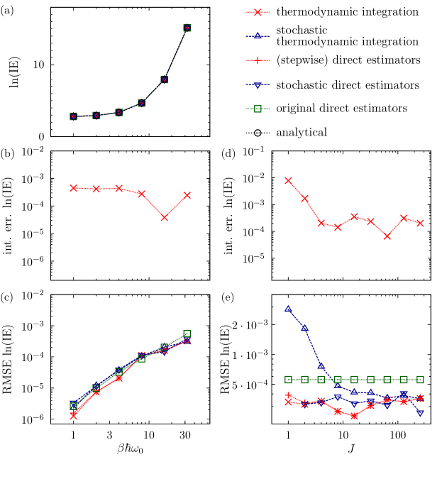
Figure 1: Isotope effect calculations in an eight-dimensional harmonic model from Ref. Karandashev and Vaníček, 2017. Results of thermodynamic integration (TI), stochastic thermodynamic integration (STI), stepwise direct estimators (DE), stochastic direct estimators (SDE), and original direct estimator (ODE) approach from Ref. Cheng and Ceriotti, 2014 are compared with exact analytical values (for the same finite Trotter number $P$). The proposed method is SDE, while DE already provide some improvement over ODE. Panels (a)-(c) show the temperature dependence of (a) the isotope effect, (b) its integration errors for TI, and (c) its statistical root mean square errors (RMSEs). Panels (d)-(e) display the dependence of integration errors (for TI) and RMSEs on the number $J$ of integration subintervals at a temperature given by $\beta\hbar\omega_{0}=32$.

III.3 Deuteration of methane

III.3.1 Computational details

As mentioned above, calculation parameters for DE, SDE, and ODE are identical to those from Ref. Karandashev and Vaníček, 2017, with a few modifications described in Subsection III.1; the TI and STI results were taken from Ref. Karandashev and Vaníček, 2017. Here we only add that the computational time spent on TI, STI, SDE, DE, and ODE calculations was approximately the same.

For each temperature we also ran calculations at $\lambda=0$ and $\lambda=1$ to estimate the path integral discretization error with the method explained in Appendix E which uses estimator $\mathcal{W}_{2}$ for $Q_{2P}/Q_{P}$. These simulations were $10^{7}$ Monte Carlo steps long, $14\%$ were whole-chain moves and $86\%$ were multi-slice moves performed on one sixth of the chain with the staging algorithmSprik, Klein, and Chandler (1985a, b) (this guaranteed that approximately the same computer time was spent on either of the two types of moves). $\mathcal{W}_{2}$ was evaluated only after each ten Monte Carlo steps to decrease the calculation cost.

III.3.2 Results and discussion

The results of the calculations of the $\mathrm{CD}_{4}/\mathrm{CH}_{4}$ isotope effect are presented in Fig. 2, with TI and STI results from Ref. Karandashev and Vaníček, 2017 plotted for comparison. Panel (a) shows that the isotope effects calculated with the five different methods described in Sec. II agree, confirming that SDE were implemented correctly, even though TI does exhibit a small integration error [see panel (b)]. Panel (c) of Fig. 2 shows that STI, SDE, TI, and DE exhibit quite similar statistical errors, while the ODE, quite surprisingly, exhibit statistical errors quite close to stepwise approaches for all but the lowest temperature. Several reasons why ODE seem to perform well for a rather large range of isotope effect values are analyzed in Appendix B.

Figure 2: $\mathrm{CD}_{4}/\mathrm{CH}_{4}$ isotope effect (IE) computed with several methods. Panels (a)-(c) show the temperature dependence of (a) the isotope effect, (b) its integration errors for thermodynamic integration, and (c) its statistical root mean square errors (RMSEs).

For reference, the SDE, DE, and ODE values plotted in Fig. 2 are listed in Table 1 together with their discretization errors estimated by the method described in Appendix E. Note that the discretization error only depends on $P$ and not on the method used for the isotope effect calculation, and that our method for estimating this discretization error exhibits favorable statistical behavior.

As mentioned in Ref. Karandashev and Vaníček, 2017, benefits of stochastically changing mass become most apparent when computational resources are limited. We therefore compared isotope effects obtained with TI, DE, STI, SDE, and ODE using simulations of increasing length, starting with very short, and hence nonergodic simulations. The results of these calculations, performed according to a prescription detailed in Ref. Karandashev and Vaníček, 2017, are plotted in Fig. 3. The general tendency is the same as was observed in Ref. Karandashev and Vaníček, 2017: approaches that require several simulations to evaluate the isotope effect (TI and DE) require more Monte Carlo steps in total to achieve converged results than those requiring only one simulation (STI, SDE, and ODE). This is due to a certain time needed for a simulation to adequately explore the $\mathbf{r}$ space; while TI and DE need to take the corresponding minimal number of Monte Carlo steps for $J$ simulations, STI, SDE, and ODE need to do it only for one simulation. For STI and SDE this benefit is slightly counteracted by introducing an extra dimension $\lambda$ to be explored by the simulation, but we have found our Monte Carlo procedure tends to explore this dimension much faster than $\mathbf{r}$ in realistic simulations; a model example, where this is not the case, is provided in Sec. II of Supplementary Material.

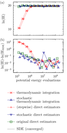
Figure 3: Impact of nonergodicity appearing in shorter calculations of the $\mathrm{CD}_{4}/\mathrm{CH}_{4}$ isotope effect (IE) at $T=200$ K. Panel (a) presents the convergence of the IE as a function of the number of potential energy evaluations needed for calculations with different simulation lengths, while panel (b) shows the corresponding error of the IE (in logarithmic scale) relative to a converged stochastic direct estimators (SDE) result. The horizontal line in panel (a) labeled “SDE (converged)” is the converged SDE result $\ln(\text{IE}_{\mathrm{SDE}})=19.785$ from Fig. 2 and Table 1; the same value was used as a reference in panel (b).

III.4 Deuteration of methanium

In this subsection we evaluate the $\mathrm{CD}_{5}^{+}/\mathrm{CH}_{5}^{+}$ isotope effect using the same techniques as for methane in Subsec. III.3 and Ref. Karandashev and Vaníček, 2017, including TI, DE, STI, SDE, ODE, and harmonic approximation; the only difference of the calculation parameters was that $J=5$ was employed for mass discretization. Potential energy surface from Ref. Jin, Braams, and Bowman, 2006 was used during the simulations.

The resulting isotope effects are plotted in Fig. 4 along with their root mean square errors and integration error for TI. As seen in panel (a), the four path integral methods that do not exhibit integration error (DE, SDE, STI, and ODE) agree with each other up to statistical error, while TI exhibits a noticeable, but rather small, integration error plotted in panel (b). Panel (c) shows root mean square errors of the isotope effect obtained with different methods. As was the case for methane, TI, DE, STI, and SDE exhibit similar statistical errors in the entire temperature range. ODE exhibit statistical errors similar to the other four methods for all temperatures but the lowest one, for which using the stepwise approach decreases the statistical error by approximately $40\%$; an analysis of why ODE perform well for isotope effects of such a large magnitude is presented in Appendix B. Isotope effect values obtained with the harmonic approximation are also plotted in panel (c) and they agree surprisingly well with exact path integral methods in this case, probably because the greatest contributions to an isotope effect tend to arise from more rigid molecular degrees of freedom (e.g., movement of the carbon atom towards one of the hydrogens), which are largely harmonic.Huang et al. (2006); Ivanov et al. (2010); Ivanov, Witt, and Marx (2013) Note that the harmonic approximation was obtained by expanding the potential energy about one of the 120 equivalent potential energy minima of $\mathrm{CH}_{5}^{+}$. For reference, all calculated isotope effects along with the estimated discretization errors are presented in Table 2.

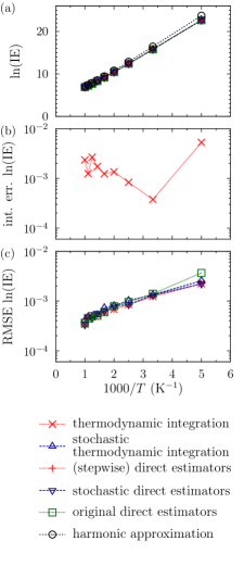
Figure 4: $\mathrm{CD}_{5}^{+}/\mathrm{CH}_{5}^{+}$ isotope effect (IE) computed with several methods. For details, see caption of Figure 2.

As in Subsec. III.3, we compared isotope effects obtained with TI, DE, STI, SDE, and ODE using simulations of increasing length, starting with very short, and hence nonergodic simulations. The results of these calculations, performed according to a prescription detailed in Ref. Karandashev and Vaníček, 2017, are plotted in Fig. 5. The general tendency is the same as was observed in Ref. Karandashev and Vaníček, 2017 and in the case of methane in Subsec. III.3: approaches that require several simulations to evaluate the isotope effect (TI and DE) require more Monte Carlo steps in total to achieve converged results than those requiring only one simulation (STI, SDE, and ODE).

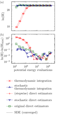
Figure 5: Impact of nonergodicity appearing in shorter calculations of the $\mathrm{CD}_{5}^{+}/\mathrm{CH}_{5}^{+}$ isotope effect (IE) at $T=200$ K. For details, see the caption of Figure 3. The horizontal line in panel (a) labeled “SDE (converged)” is the converged SDE result $\ln(\text{IE}_{\mathrm{SDE}})=22.674$ from Fig. 4 and Table 2; the same value was used as a reference in panel (b).

Table 1: Values of the $\mathrm{CD}_{4}/\mathrm{CH}_{4}$ isotope effect (IE) obtained with direct estimators (DE), “stochastic direct estimators” (SDE), and “original direct estimators” (ODE) (for other values seen in Fig. 2, see Ref. Karandashev and Vaníček, 2017). The proposed methodology is SDE. The discretization error is defined as $\mathrm{IE}_{P}/\mathrm{IE}-1$ and is estimated with the procedure described in Appendix E.

$T(\text{K})$	$P$	ln(IE) ($\mathrm{CD_{4}/CH_{4}}$) with statistical error			Estimate of
		DE	SDE	ODE	discretization error ($10^{-3}$)
0200	360	$19.786\pm 0.002$	$19.785\pm 0.002$	$19.790\pm 0.003$	$-5.1\pm 0.3$
0300	226	$13.672\pm 0.002$	$13.672\pm 0.001$	$13.673\pm 0.001$	$-3.7\pm 0.2$
0400	158	$10.666\pm 0.001$	$10.667\pm 0.001$	$10.666\pm 0.001$	$-3.2\pm 0.2$
0500	118	$\phantom{0}8.910\pm 0.001$	$\phantom{0}8.910\pm 0.001$	$\phantom{0}8.909\pm 0.001$	$-3.0\pm 0.2$
0600	090	$\phantom{0}7.780\pm 0.001$	$\phantom{0}7.780\pm 0.001$	$\phantom{0}7.780\pm 0.001$	$-3.0\pm 0.2$
0700	072	$\phantom{0}7.006\pm 0.001$	$\phantom{0}7.005\pm 0.001$	$\phantom{0}7.007\pm 0.001$	$-2.8\pm 0.2$
0800	058	$\phantom{0}6.451\pm 0.001$	$\phantom{0}6.450\pm 0.001$	$\phantom{0}6.451\pm 0.001$	$-2.8\pm 0.2$
0900	046	$\phantom{0}6.039\pm 0.001$	$\phantom{0}6.039\pm 0.001$	$\phantom{0}6.038\pm 0.001$	$-3.4\pm 0.2$
1000	036	$\phantom{0}5.725\pm 0.001$	$\phantom{0}5.726\pm 0.001$	$\phantom{0}5.725\pm 0.001$	$-3.9\pm 0.2$

Table 2: Values of the $\mathrm{CD}_{5}^{+}/\mathrm{CH}_{5}^{+}$ isotope effect (IE) obtained with several different methods. For details, see the caption of Table 1. The values of $P$ for a given temperature were the same as those for methane listed in Table 1.

$T(\text{K})$	ln(IE) ($\mathrm{CD_{5}^{+}/CD_{5}^{+}}$)						Estimate of discretization error ($10^{-3}$)
	Path integral values with statistical errors					harmonic approximation
	TI	DE	STI	SDE	ODE
0200	$22.669\pm 0.003$	$22.669\pm 0.003$	$22.671\pm 0.003$	$22.674\pm 0.003$	$22.665\pm 0.004$	$23.727$	$-5.0\pm 0.3$
0300	$15.789\pm 0.002$	$15.790\pm 0.002$	$15.790\pm 0.002$	$15.789\pm 0.002$	$15.790\pm 0.002$	$16.446$	$-3.9\pm 0.3$
0400	$12.411\pm 0.001$	$12.412\pm 0.001$	$12.410\pm 0.001$	$12.410\pm 0.001$	$12.413\pm 0.001$	$12.875$	$-3.5\pm 0.3$
0500	$10.443\pm 0.001$	$10.444\pm 0.001$	$10.445\pm 0.001$	$10.444\pm 0.001$	$10.443\pm 0.001$	$10.796$	$-3.1\pm 0.2$
0600	$\phantom{0}9.181\pm 0.001$	$\phantom{0}9.183\pm 0.001$	$\phantom{0}9.183\pm 0.001$	$\phantom{0}9.182\pm 0.001$	$\phantom{0}9.183\pm 0.001$	$\phantom{0}9.461$	$-3.0\pm 0.2$
0700	$\phantom{0}8.319\pm 0.001$	$\phantom{0}8.321\pm 0.001$	$\phantom{0}8.321\pm 0.001$	$\phantom{0}8.321\pm 0.001$	$\phantom{0}8.321\pm 0.001$	$\phantom{0}8.549$	$-2.7\pm 0.2$
0800	$\phantom{0}7.703\pm 0.001$	$\phantom{0}7.705\pm 0.001$	$\phantom{0}7.705\pm 0.001$	$\phantom{0}7.706\pm 0.001$	$\phantom{0}7.704\pm 0.001$	$\phantom{0}7.896$	$-3.1\pm 0.2$
0900	$\phantom{0}7.248\pm 0.001$	$\phantom{0}7.250\pm 0.001$	$\phantom{0}7.249\pm 0.001$	$\phantom{0}7.249\pm 0.001$	$\phantom{0}7.250\pm 0.001$	$\phantom{0}7.414$	$-3.7\pm 0.2$
1000	$\phantom{0}6.902\pm 0.001$	$\phantom{0}6.904\pm 0.001$	$\phantom{0}6.905\pm 0.001$	$\phantom{0}6.905\pm 0.001$	$\phantom{0}6.905\pm 0.001$	$\phantom{0}7.048$	$-4.1\pm 0.2$

IV Conclusion

In this paper, we continued our program of accelerating the calculations of equilibrium isotope effects. Starting from a basic idea of thermodynamic integration with respect to mass,Vaníček et al. (2005) one can 1) accelerate statistical convergence by using centroid virial estimators, which, in the case of path integral Monte Carlo avoid evaluating forces by employing a finite-difference derivative trick,Vaníček and Miller (2007); Zimmermann and Vaníček (2009) 2) accelerate convergence to the quantum limit by employing higher-order factorizations of the path integral,Buchowiecki and Vaníček (2013) and 3) reduce or remove the error of thermodynamic integration, which was the focus of the present work.

To remove the thermodynamic integration error, we investigated optimal ways to use direct estimatorsPérez and von Lilienfeld (2011); Cheng and Ceriotti (2014) for larger isotope effects. First, we introduced a near optimal way to discretize the larger isotope effect into smaller ones, and showed that the statistical error of the resulting method was quite close to the corresponding error exhibited by thermodynamic integration. Second, we showed how statistical convergence of the method could be improved by combining it with the stochastic change of mass. We referred to the resulting method as the “stochastic direct estimators.”

We also observed that simple, original application of the mass-scaled direct estimators proposed in Ref. Cheng and Ceriotti, 2014 performed well for isotope effects of surprisingly large magnitudes. These results, combined with our discussion of the method’s convergence and divergence in Appendix B, indicate that the applicability of the direct estimators could be broader than what had been reported before. In the end, the approach of Ref. Cheng and Ceriotti, 2014 can be quite efficient for isotope effects much larger than unity, especially if the system in question allows to capitalize on atom interchangeability. Yet, for the largest isotope effects using stochastic direct estimators is still preferable, as indicated by our results for the deuterization of methane and methanium at lower temperatures.

The way we used mass-scaled normal modes to define mass-scaled $\lambda$-moves can be extended to any mapping used in targeted free energy perturbationJarzynski (2002) provided the mapping is non-local. In this context our results compare using the same physically-motivated mapping either to perform a free energy perturbation calculation (original direct estimators) or to define an analogue of our Monte Carlo procedure and combine it with thermodynamic integration or stepwise free energy perturbation. The quality of the mapping affects statistical errors of the first approach through dispersion of the free energy perturbation estimator; in the second approach estimator properties are less affected, but an inefficient procedure for sampling $\lambda$ can increase correlation length of the samples. Our results for methane and methanium at lower temperatures illustrate how the second approach is less affected by the quality of the mapping.

Finally, let us mention that stochastic direct estimators can be combined with the Takahashi-Imada or Suzuki fourth-order factorizationsTakahashi and Imada (1984); Suzuki (1995); Chin (1997); Jang, Jang, and Voth (2001) of the Boltzmann operator, which would allow lowering the path integral discretization error of the computed isotope effect for a given Trotter number $P$, and hence a faster convergence to the quantum limit.Pérez and Tuckerman (2011); Buchowiecki and Vaníček (2013); Maršálek et al. (2014); Karandashev and Vaníček (2015)

Supplementary material

Section I of Supplementary Material describes an alternative procedure, in which several isotope effects are evaluated simultaneously. Examples include four isotope effects of the form $\mathrm{CH_{4-x}D_{x}/CH_{4}}$ (x$=1,\ldots,4$) and five isotope effects $\mathrm{CH_{5-x}D_{x}^{+}/CH_{5}^{+}}$ ($\mathrm{x}=1,\ldots,5$). Section II analyzes effects of nonergodicity on isotope effect calculations in the harmonic model.

Appendix A Statistical errors, convergence, and divergence of direct estimators for an isotope effect in a harmonic system

In this appendix we derive $P\rightarrow\infty$ limits of root mean square errors (RMSEs) of direct estimators $\mathcal{Z}_{\mathrm{th}}$ and $\mathcal{Z}_{\mathrm{sc}}$ for a harmonic system. For simplicity, the system is defined as $N$ particles with masses $m_{i}$ moving in one-dimensional Cartesian space, the corresponding oscillator frequencies being $\omega_{i}$. We are mainly interested in the relative statistical error of $A$, that is $\Delta A/A$, where

$$\Delta A=\sqrt{\langle A^{2}\rangle-\langle A\rangle^{2}}$$ (18)

is the RMSE of $A$ and $\langle X\rangle$ denotes an average over all samples of $X$. To simplify the analytical derivation, instead of $\Delta A/A$, we will evaluate the quantity

$$\left(\frac{\Delta A}{A}\right)^{2}+1=\frac{\langle A^{2}\rangle}{\langle A\rangle^{2}}.$$ (19)

For a direct estimator $\mathcal{Z}^{0,1}$ this ratio takes the form

$$\frac{\langle(\mathcal{Z}^{0,1})^{2}\rangle^{(0)}}{(\langle\mathcal{Z}^{0,1}\rangle^{(0)})^{2}}=\frac{Q(0)\int(\mathcal{Z}^{0,1})^{2}\rho^{(0)}(\mathbf{r})d\mathbf{r}}{[Q(1)]^{2}}.$$ (20)

For $\mathcal{Z}_{\mathrm{th}}^{0,1},$ we have

$$\begin{split}\int(\mathcal{Z}_{\mathrm{th}}^{0,1})^{2}\rho^{(0)}(\mathbf{r})d\mathbf{r}=&C\int d\mathbf{r\,}\left[\prod_{i=1}^{N}\frac{m_{i}(1)}{m_{i}(0)}\right]^{P}\\ &\times\exp\left\{\frac{P}{2\beta\hbar^{2}}\sum_{i=1}^{N}[m_{i}(0)-2m_{i}(1)]\sum_{s=1}^{P}|\mathrm{r}_{i}^{(s)}-\mathrm{r}_{i}^{(s-1)}|^{2}-\frac{\beta}{P}\sum_{s=1}^{P}V(\mathbf{r}^{(s)})\right\}\end{split}$$ (21)

$$\begin{split}=&\left(\prod_{i=1}^{N}\left\{1+\frac{[m_{i}(1)-m_{i}(0)]^{2}}{m_{i}(0)[2m_{i}(1)-m_{i}(0)]}\right\}\right)^{P/2}\left(\frac{P}{2\pi\beta\hbar^{2}}\right)^{NP/2}\left\{\prod_{i=1}^{N}[2m_{i}(1)-m_{i}(0)]\right\}^{P/2}\\ &\times\int\exp\left\{-\frac{P}{2\beta\hbar^{2}}\sum_{i=1}^{N}[2m_{i}(1)-m_{i}(0)]\sum_{s=1}^{P}|\mathrm{r}_{i}^{(s)}-\mathrm{r}_{i}^{(s-1)}|^{2}-\frac{\beta}{P}\sum_{s=1}^{P}V(\mathbf{r}^{(s)})\right\}d\mathbf{r}.\end{split}$$ (22)

If $m_{i}(0)>2m_{i}(1)$ for some $i$, then the first term in the argument of the exponential becomes positive and for large enough values of $P$ the integral over $\mathbf{r}$ starts to diverge; this can be easily seen after rewriting it in terms of mass-scaled normal modes (see Appendix A of Ref. Karandashev and Vaníček, 2017). If $m_{i}(0)<2m_{i}(1)$, then interpreting the integral over $\mathbf{r}$ as the path integral representation of the partition function (3) for a harmonic system with rescaled masses reveals the limiting behavior

$$\begin{split}\lim_{P\rightarrow\infty}\int(\mathcal{Z}_{\mathrm{th}}^{0,1})^{2}\rho^{(0)}(\mathbf{r})d\mathbf{r}&=\lim_{P\rightarrow\infty}\prod_{i=1}^{N}\frac{\left\{1+[m_{i}(1)-m_{i}(0)]^{2}/m(0)/[2m_{i}(1)-m_{i}(0)]\right\}^{P/2}}{2\sinh\left(\beta\hbar\omega_{i}\sqrt{m(0)/[2m_{i}(1)-m_{i}(0)]}/2\right)}\\ &=+\infty,\end{split}$$ (23)

implying the divergence of the statistical error of the thermodynamic direct estimator, consistent with the similar divergence of the “thermodynamic free energy perturbation” estimator of Ref. Ceriotti and Markland, 2013. For $\mathcal{Z}_{\mathrm{sc}}^{0,1}$, we have

$$\begin{split}\int(\mathcal{Z}_{\mathrm{sc}}^{0,1})^{2}\rho(\mathbf{r})d\mathbf{r}=C\left[\prod_{i=1}^{N}\frac{m_{i}(1)}{m_{i}(0)}\right]\int d\mathbf{r}\exp\left\{-\frac{P}{2\beta\hbar^{2}}\sum_{i=1}^{N}m_{i}(0)\sum_{s=1}^{P}|\mathrm{r}_{i}^{(s)}-\mathrm{r}_{i}^{(s-1)}|^{2}-\frac{\beta}{P}\sum_{s=1}^{P}\left[2V(\mathbf{r}_{0,1}^{(s)})-V(\mathbf{r}^{(s)})\right]\right\}.\end{split}$$ (24)

To simplify this expression, let us rewrite it in terms of mass-scaled normal modes $\mathbf{u}$ (see Appendix A of Ref. Karandashev and Vaníček, 2017). We will only consider the case of an even $P$, with the case of odd $P$ being completely analogous. For a harmonic system, we have

$$\begin{split}\frac{1}{P}\sum_{s=1}^{P}V(\mathbf{r}^{(s)})&=\sum_{i=1}^{N}\frac{m_{i}(0)\omega_{i}^{2}}{2P}\sum_{s=1}^{P}|\mathrm{r}_{i}^{(s)}|^{2}\\ &=\sum_{i=1}^{N}\omega_{i}^{2}\left[\frac{m_{i}(0)|\mathrm{r}_{i}^{(C)}|^{2}}{2}+\frac{|a_{i}^{(P/2)}|^{2}}{2}+\sum_{k=1}^{P/2-1}(|a_{i}^{(k)}|^{2}+|b_{i}^{(k)}|^{2})\right],\end{split}$$ (25)

and recalling the expression (15) for $\mathbf{r}_{0,1}^{(s)}$ in terms of mass-scaled normal modes yields

$$\frac{1}{P}\sum_{s=1}^{P}V(\mathbf{r}_{0,1}^{(s)})=\sum_{i=1}^{N}\omega_{i}^{2}\frac{m_{i}(0)}{m_{i}(1)}\left[\frac{m_{i}(1)|\mathrm{r}_{i}^{(C)}|^{2}}{2}+\frac{|a_{i}^{(P/2)}|^{2}}{2}+\sum_{k=1}^{P/2-1}(|a_{i}^{(k)}|^{2}+|b_{i}^{(k)}|^{2})\right].$$ (26)

Combining this with the expression for the effective potential $\tilde{\Phi}(\mathbf{u})$ (see Appendix A of Ref. Karandashev and Vaníček, 2017) leads to

$$\begin{split}\int(\mathcal{Z}_{\mathrm{sc}}^{0,1})^{2}\rho(\mathbf{u})d\mathbf{u}=&\left[\prod_{i=1}^{N}\frac{m_{i}(1)}{m_{i}(0)}\right]\tilde{C}\int d\mathbf{r}^{(C)}\exp\left[-\beta\sum_{i=1}^{N}\frac{m_{i}(0)\omega_{i}^{2}|\mathrm{r}_{i}^{(C)}|^{2}}{2}\right]\\ &\times\int d\mathbf{a}^{(P/2)}\exp\left\{-\frac{2P^{2}|\mathbf{a}^{(P/2)}|^{2}}{\beta\hbar^{2}}-\beta\sum_{i=1}^{N}\frac{\omega_{i}^{2}|\mathrm{a}_{i}^{(P/2)}|^{2}}{2}\left[2\frac{m_{i}(0)}{m_{i}(1)}-1\right]\right\}\\ &\times\prod_{k=1}^{P/2-1}\int d\mathbf{a}^{(k)}d\mathbf{b}^{(k)}\exp\left\{-\frac{2P^{2}}{\beta\hbar^{2}}\left(1-\cos\frac{2\pi k}{P}\right)(|\mathbf{a}^{(k)}|^{2}+|\mathbf{b}^{(k)}|^{2})\right.\\ &\left.-\beta\sum_{i=1}^{N}\frac{\omega_{i}^{2}(|\mathrm{a}_{i}^{(k)}|^{2}+|\mathrm{b}_{i}^{(k)}|^{2})}{2}\left[2\frac{m_{i}(0)}{m_{i}(1)}-1\right]\right\}.\end{split}$$ (27)

If $m_{i}(1)>2m_{i}(0)$ for some $i$, then for large enough $\omega_{i}$ the expression will diverge, implying the divergence of the statistical error of the mass-scaled direct estimator. Otherwise rescaling each $\mathrm{r}_{i}^{(C)}$ by a factor of $\sqrt{2m_{i}(0)/m_{i}(1)-1}$ and comparing the resulting expression to $Q_{P}$ rewritten in terms of $\mathbf{u}$ yields

$$\lim_{P\rightarrow\infty}\int(\mathcal{Z}_{\mathrm{sc}}^{0,1})^{2}\rho(\mathbf{u})d\mathbf{u}=\prod_{i=1}^{N}\left\{\frac{m_{i}(1)}{m_{i}(0)}\frac{\sqrt{2m_{i}(0)/m_{i}(1)-1}}{2\sinh(\beta\hbar\omega_{i}\sqrt{2m_{i}(0)/m_{i}(1)-1}/2)}\right\}$$ (28)

We now introduce the function

$$f_{i}(x)=\frac{\sqrt{x}}{2\sinh(\beta\hbar\sqrt{k_{i}x}/2)},$$ (29)

where $k_{i}$ is the force constant for the $i$th degree of freedom, in order to rewrite expression (20) in the limit $P\rightarrow\infty$ as

$$\frac{\langle(\mathcal{Z}_{\mathrm{sc}}^{0,1})^{2}\rangle^{(0)}}{(\langle\mathcal{Z}_{\mathrm{sc}}^{0,1}\rangle^{(0)})^{2}}=\prod_{i=1}^{N}\frac{f_{i}[1/m_{i}(0)]f_{i}[2/m_{i}(1)-1/m_{i}(0)]}{\{f_{i}[1/m_{i}(1)]\}^{2}}.$$ (30)

Since $f_{i}(x)$ is a monotonously decreasing function of $x$ for each $i=1,\ldots,N$, it is straightforward to show that if $m_{i}(0)<m_{i}(1)$ for all $i=1,\ldots,N$, then the identity (30) implies the inequality

$$\frac{\langle(\mathcal{Z}_{\mathrm{sc}}^{1,0})^{2}\rangle^{(1)}}{(\langle\mathcal{Z}_{\mathrm{sc}}^{1,0}\rangle^{(1)})^{2}}<\frac{\langle(\mathcal{Z}_{\mathrm{sc}}^{0,1})^{2}\rangle^{(0)}}{(\langle\mathcal{Z}_{\mathrm{sc}}^{0,1}\rangle^{(0)})^{2}}.$$ (31)

This final inequality proves, for harmonic systems, an observation from Ref. Cheng and Ceriotti, 2014: If one evaluates an isotope effect in a harmonic system using direct estimators for the isotope effect, then running a path integral simulation at the larger value of mass leads to smaller statistical errors than running the simulation at the lower value of mass.

Appendix B Sufficient conditions for the convergence of direct estimators for isotope substitution

In this appendix we discuss several sufficient conditions that guarantee that direct estimators exhibit a finite root mean square error. For $\mathcal{Z}_{\mathrm{th}}^{0,1}$ this is obviously the case if $2m_{i}(1)\geq m_{i}(0)$ for all $i=1,\ldots,N$, as in this case the path integral appearing in Eq. (21) will have an upper bound of

$$\int(\mathcal{Z}_{\mathrm{th}}^{0,1})^{2}\rho^{(0)}(\mathbf{r})d\mathbf{r}\leq C\left[\prod_{i=1}^{N}\frac{m_{i}(1)}{m_{i}(0)}\int e^{-\beta V(\mathbf{r}^{(1)})/P}d\mathbf{r}^{(1)}\right]^{P}.$$ (32)

This upper bound goes to infinity as $P\rightarrow\infty$, as should be expected from $\mathcal{Z}_{\mathrm{th}}^{0,1}$ exhibiting an infinitely large statistical error in this limit. For $\mathcal{Z}_{\mathrm{sc}}^{0,1}$, we start by noting that the root mean square error of a bound observable is always finite, which is obviously the case if the potential function $V$ itself is bound. $\mathcal{Z}_{\mathrm{sc}}^{0,1}$ is also bound if $V$ is convex and $m_{i}(0)>m_{i}(1)$ for all $i=1,\ldots,N$. Indeed, for a given $s=1,\ldots,P$

$$V(\mathbf{r}^{(s)})-V(\mathbf{r}^{(s)}_{0,1})\leq\nabla V(\mathbf{r}^{(s)})\cdot(\mathbf{r}^{(s)}-\mathbf{r}^{(s)}_{0,1}),$$ (33)

which follows from $V(\mathbf{r}^{(s)})$ being a convex function of one variable when change along the direction $\mathbf{r}^{(s)}-\mathbf{r}^{(s)}_{0,1}$ is considered. From the definition (15) of $\mathbf{r}^{(s)}_{0,1}$ we obtain a positive definite matrix $\mathbf{A}$ such that

$$\mathbf{r}^{(s)}-\mathbf{r}^{(s)}_{0,1}=\mathbf{A}\cdot(\mathbf{r}^{(s)}-\mathbf{r}^{(C)}).$$ (34)

We also introduce

$$\tilde{\mathbf{r}}^{(s)}(\tau)=\tau\mathbf{r}^{(s)}+(1-\tau)\mathbf{r}^{(C)}$$ (35)

and write

$$\begin{split}\nabla V(\mathbf{r}^{(s)})\cdot\mathbf{A}\cdot(\mathbf{r}^{(s)}-\mathbf{r}^{(C)})=&\nabla V(\mathbf{r}^{(C)})\cdot\mathbf{A}\cdot(\mathbf{r}^{(s)}-\mathbf{r}^{(C)})+\int_{0}^{1}d\tau(\mathbf{r}^{(s)}-\mathbf{r}^{(C)})\cdot\left(\mathbf{A}\left.\frac{\partial^{2}V(\mathbf{r}^{(s)})}{\partial(\mathbf{r}^{(s)})^{2}}\right|_{\mathbf{r}^{(s)}=\tilde{\mathbf{r}}^{(s)}(\tau)}\right)\cdot(\mathbf{r}^{(s)}-\mathbf{r}^{(C)}).\end{split}$$ (36)

Since $V$ is a convex function, $\partial^{2}V(\mathbf{r}^{(s)})/\partial(\mathbf{r}^{(s)})^{2}$ is a positive semi-definite matrix, and therefore $\mathbf{A}\partial^{2}V(\mathbf{r}^{(s)})/\partial(\mathbf{r}^{(s)})^{2}$ has non-negative eigenvalues. Thus, for each $\tau$

$$(\mathbf{r}^{(s)}-\mathbf{r}^{(C)})\cdot\left(\mathbf{A}\left.\frac{\partial^{2}V(\mathbf{r}^{(s)})}{\partial(\mathbf{r}^{(s)})^{2}}\right|_{\mathbf{r}^{(s)}=\tilde{\mathbf{r}}^{(s)}(\tau)}\right)\cdot(\mathbf{r}^{(s)}-\mathbf{r}^{(C)})\geq 0.$$ (37)

Combining Eqs. (33), (36), and (37), then summing the result over $s$ leads us to

$$\sum_{s=1}^{P}[V(\mathbf{r}^{(s)})-V(\mathbf{r}^{(s)}_{0,1})]\leq\nabla V(\mathbf{r}^{(C)})\cdot\mathbf{A}\cdot\sum_{s=1}^{P}(\mathbf{r}^{(s)}-\mathbf{r}^{(C)})=0,$$ (38)

proving that in this case $\mathcal{Z}_{\mathrm{sc}}^{0,1}$ is bound in a way that does not depend on $P$

$$\mathcal{Z}_{\mathrm{sc}}^{0,1}\leq\left[\prod_{i=1}^{N}\frac{m_{i}(1)}{m_{i}(0)}\right]^{D/2}.$$ (39)

Appendix C Optimal choice of mass discretization and reference masses for the stepwise application of direct estimators

In this appendix we discuss choices of $\lambda_{j}$ and $\overline{\lambda}_{j}$ that minimize the root mean square error of the direct estimator expression (17). In other words, we discuss the optional choice of the partition of the interval $[0,1]$ into subintervals $[\lambda_{j-1},\lambda_{j}]$ and the optimal choice of the reference masses $(\overline{\lambda}_{j})$ in each of the subintervals $[\lambda_{j-1},\lambda_{j}]$.

The first part of the problem is the choice of $\overline{\lambda}$ that minimizes the statistical error of the ratio $\langle\mathcal{Z}_{\mathrm{sc}}^{\overline{\lambda},1}\rangle^{(\overline{\lambda})}/\langle\mathcal{Z}_{\mathrm{sc}}^{\overline{\lambda},0}\rangle^{(\overline{\lambda})}$. Estimating the root mean square error of this ratio analytically is problematic as the averages are obtained from the same Monte Carlo trajectory, and hence are correlated. Even if one could neglect the correlation between the two averages, the resulting estimate for an optimal $\overline{\lambda}$ value would be too complicated to be useful. Yet, we can suggest two rules of thumb based on an approximate behavior in the deep quantum regime because the most quantum degrees of freedom typically contribute the most to the statistical error. [Equation (30) can be shown to imply this.] For simplicity let us consider a one-dimensional harmonic oscillator with force constant $k$, mass changed from $m(0)$ to $m(1)>m(0)$, and $m(\lambda)$ given by the inverse square root interpolation formula (7). Assuming the averages of $\mathcal{Z}_{\mathrm{sc}}^{\overline{\lambda},1}$ and $\mathcal{Z}_{\mathrm{sc}}^{\overline{\lambda},0}$ to be approximately independent and to have the limiting behavior of Eq. (20) at low temperatures allows us to write

$$\begin{split}\left[\frac{\Delta(\langle\mathcal{Z}_{\mathrm{sc}}^{\overline{\lambda},1}\rangle^{(\overline{\lambda})}/\langle\mathcal{Z}_{\mathrm{sc}}^{\overline{\lambda},0}\rangle^{(\overline{\lambda})})}{\langle\mathcal{Z}_{\mathrm{sc}}^{\overline{\lambda},1}\rangle^{(\overline{\lambda})}/\langle\mathcal{Z}_{\mathrm{sc}}^{\overline{\lambda},0}\rangle^{(\overline{\lambda})}}\right]^{2}\approx\,\,\,\,\,\,\,&\left[\frac{\langle(\mathcal{Z}_{\mathrm{sc}}^{\overline{\lambda},1})^{2}\rangle}{\langle\mathcal{Z}_{\mathrm{sc}}^{\overline{\lambda},1}\rangle^{2}}+\frac{\langle(\mathcal{Z}_{\mathrm{sc}}^{\overline{\lambda},0})^{2}\rangle}{\langle\mathcal{Z}_{\mathrm{sc}}^{\overline{\lambda},0}\rangle^{2}}-2\right]\\ \stackrel{{\scriptstyle\mathclap{\mbox{\footnotesize$\beta\rightarrow\infty$}}}}{{\sim}}\,\,\,\,\,\,\,&\frac{\sqrt{m(1)[2m(\overline{\lambda})-m(1)]}}{m(\overline{\lambda})}\exp\left\{\beta\hbar\sqrt{k}\left[\frac{1}{\sqrt{m(1)}}-\frac{1}{2\sqrt{m(\overline{\lambda})}}-\frac{1}{2}\sqrt{\frac{2}{m(1)}-\frac{1}{m(\overline{\lambda})}}\right]\right\}\\ &+\frac{\sqrt{m(0)[2m(\overline{\lambda})-m(0)]}}{m(\overline{\lambda})}\exp\left\{\beta\hbar\sqrt{k}\left[\frac{1}{\sqrt{m(0)}}-\frac{1}{2\sqrt{m(\overline{\lambda})}}-\frac{1}{2}\sqrt{\frac{2}{m(0)}-\frac{1}{m(\overline{\lambda})}}\right]\right\}.\end{split}$$ (40)

We also assume that $\mathcal{Z}_{\mathrm{sc}}^{\overline{\lambda},1}$ does not exhibit a divergent behavior [as described in Appendix A], since it could only appear in this problem for very exotic mass differences [$m(1)>2m(0)$] and a too sparse discretization into $\lambda$ subintervals. In the $\beta\rightarrow\infty$ limit, differentiating either term in (40) with respect to $\overline{\lambda}$ and dividing the result by $\beta\mathrm{d}m(\overline{\lambda})/\mathrm{d}\overline{\lambda}$ leads to an expression whose magnitude in the $\beta\rightarrow\infty$ limit will be mainly determined by the argument of the exponential. The minimum corresponds to derivatives of the two terms having the same magnitude to cancel out, which implies the arguments of the two exponentials being approximately equal. Straightforward algebra indicates the argument of the first exponent is larger than in the second one at $\overline{\lambda}=1/2$, while the inequality is reversed at $\overline{\lambda}=1$, implying that the minimum lies in the interval $[1/2,1]$, which is consistent with the optimal $\bar{\lambda}$ value found in test calculations we have performed with several harmonic systems. We have not observed a significant difference between statistical errors obtained for $\overline{\lambda}=1/2$ or $\overline{\lambda}=1$ in a wide range of situations; in the limit of large $J$, however, picking $\overline{\lambda}=1/2$ becomes numerically identical to performing thermodynamic integration with the midpoint rule, while choosing $\overline{\lambda}=1$ would correspond to the right hand rule, which should lead to worse performance. $\overline{\lambda}=1/2$ was therefore the choice used in this work.

To illustrate our estimate for the optimal $\overline{\lambda}$, in Fig. 6 we plot root mean square error of $\langle\mathcal{Z}^{\overline{\lambda},1}\rangle^{(\overline{\lambda})}/\langle\mathcal{Z}^{\overline{\lambda},0}\rangle^{(\overline{\lambda})}$ as a function of $\overline{\lambda}$ for the same harmonic system as in Subsection III.2 with $\beta\hbar\omega_{0}=32$. Evidently, the optimal $\overline{\lambda}$ is in the interval $[1/2,1]$ and is quite close to $1/2$.

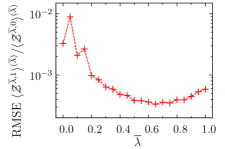
Figure 6: Relative root mean square error (RMSE) of $\langle\mathcal{Z}^{\overline{\lambda},1}\rangle^{(\overline{\lambda})}/\langle\mathcal{Z}^{\overline{\lambda},0}\rangle^{(\overline{\lambda})}$ as a function of $\overline{\lambda}$ for the harmonic system used in Ref. Karandashev and Vaníček, 2017 with $\beta\hbar\omega_{0}=32$.

We will now discuss the best way to partition a large isotope effect into smaller isotope effects, each of which can be evaluated with the original direct estimators. Assuming that the midpoint was used for an evaluation of an intermediate isotope effect $Q(\lambda^{\prime\prime})/Q(\lambda^{\prime})$ one can obtain the following approximate upper bound for the relative statistical error in the low temperature limit

$$\left[\frac{\Delta(\langle\mathcal{Z}_{\mathrm{sc}}^{\overline{\lambda},1}\rangle^{(\overline{\lambda})}/\langle\mathcal{Z}_{\mathrm{sc}}^{\overline{\lambda},0}\rangle^{(\overline{\lambda})})}{\langle\mathcal{Z}_{\mathrm{sc}}^{\overline{\lambda},1}\rangle^{(\overline{\lambda})}/\langle\mathcal{Z}_{\mathrm{sc}}^{\overline{\lambda},0}\rangle^{(\overline{\lambda})}}\right]^{2}\lesssim_{\beta\rightarrow\infty}\exp\left\{\frac{\beta\hbar\sqrt{k}}{2}\left[\frac{1}{\sqrt{m(0)}}-\frac{1}{\sqrt{m(1)}}\right]\right\}\approx\frac{Q(1)}{Q(0)}.$$ (41)

In this approximation the problem of minimizing statistical error of a “stepwise” direct estimator isotope effect calculation is equivalent to minimizing a sum of positive terms whose product is fixed. Since the solution of the latter problem requires all terms of the sum being equal, the resulting rule of thumb is to pick the intermediate isotope effects approximately equal in magnitude. In the low temperature limit, and with mass interpolation (7), this is equivalent to having the intermediate isotope effects correspond to $\lambda$ subintervals of equal size. To check this estimate we ran some test calculations for the same system as in Subsection III.2 with $\beta\hbar\omega_{0}=32$ using direct estimators and $J=2$ with different values of $\lambda_{1}$. The resulting root mean square errors are plotted in Fig. 7; for this rather quantum harmonic oscillator root mean square error is indeed minimized if $\lambda_{1}$ is close to $1/2$.

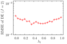
Figure 7: Relative root mean square error (RMSE) of the isotope effect evaluated with direct estimators [DE, Eq. (17)] with $J=2$ as a function of $\lambda_{1}$ for the harmonic system used in Ref. Karandashev and Vaníček, 2017 with $\beta\hbar\omega_{0}=32$.

Appendix D Details of combining direct estimators with stochastic change of mass

The procedure for changing masses between discrete values $\overline{\lambda}_{j}$ of $\lambda$ for SDE is mostly the same as the one described for STI in Subsection II C of Ref. Karandashev and Vaníček, 2017, but for two important differences. First, the umbrella potential $U_{b}(\lambda)$ is now updated in such a way that it satisfies for all $j=1,\ldots J-1$ the condition

$$\exp\{\beta[U_{b}(\overline{\lambda}_{j})-U_{b}(\overline{\lambda}_{j+1})]\}=\frac{\langle\mathcal{Z}_{\mathrm{sc}}^{\overline{\lambda}_{j+1},\lambda_{j}}\rangle^{(\overline{\lambda}_{j+1})}}{\langle\mathcal{Z}_{\mathrm{sc}}^{\overline{\lambda}_{j},\lambda_{j}}\rangle^{(\overline{\lambda}_{j})}}$$ (42)

in order to minimize the statistical error of the calculated isotope effect. Second, since the evaluation of the acceptance criterion for the simple $\lambda$-move appearing in Eq. (23) of Ref. Karandashev and Vaníček, 2017 is computationally inexpensive and we only need to consider a finite (and typically small) number of $\lambda$-values, it is possible to include the acceptance probability into the trial distribution, leading to the following procedure:

Simple $\lambda$-move:

1. For each $j=1,\ldots,J$ calculate:

   $$\begin{split}p_{j}=&\left[\prod_{i=1}^{N}m_{i}(\overline{\lambda}_{j})\right]\\ &\times\exp\left[-\frac{P}{2\beta\hbar^{2}}\sum_{i=1}^{N}m_{i}(\overline{\lambda}_{j})\sum_{s=1}^{P}|\mathrm{r}_{i}^{(s)}-\mathrm{r}_{i}^{(s-1)}|^{2}\right.\\ &\left.\vphantom{-\frac{P}{2\beta\hbar^{2}}\sum_{i=1}^{N}m_{i}(\overline{\lambda}_{j})\sum_{s=1}^{P}|\mathrm{r}_{i}^{(s)}-\mathrm{r}_{i}^{(s-1)}|^{2}}-\beta U_{b}(\overline{\lambda}_{j})\right]\end{split}$$ (43)

   $$\tilde{p}_{j}= \frac{\sum_{j^{\prime}=1}^{j}p_{j^{\prime}}}{\sum_{j^{\prime}=1}^{J}p_{j^{\prime}}}$$ (44)

2. Choose a random number $\Delta$ distributed uniformly over $[0,1]$.

3. Choose $j^{\prime}$ which is the smallest integer satisfying

   $$\Delta<\tilde{p}_{j^{\prime}}.$$ (45)

4. Set $j=j^{\prime}$, $\lambda=\overline{\lambda}_{j^{\prime}}$.

It was mentioned in Subsection II C of Ref. Karandashev and Vaníček, 2017 that simple $\lambda$-moves used for stochastic thermodynamic integration cannot lead to large changes of $\lambda$ as the corresponding acceptance ratio [Eq. (23) of Ref. Karandashev and Vaníček, 2017, which is basically the ratio of two different $p_{j}$ from Eq. (43)] exhibits a maximum which becomes sharper with larger values of $P$. We note that the SDE variant of the procedure outlined above cannot address this issue, as the smallest $\lambda$ step one can make is limited by $J$, and therefore becomes less efficient at lower temperatures.

Finally, as for the mass-scaled $\lambda$-move, the only difference from the procedure for STI in Ref. Karandashev and Vaníček, 2017 is that, in the case of SDE, the trial $\lambda$ values [Eq. (24) Ref. Karandashev and Vaníček, 2017] are picked not from the entire $[0,1]$ interval, but only from among the reference $\overline{\lambda}_{j}$ values.

Appendix E Estimate of the relative path integral discretization error

To estimate the discretization error of the path integral representation $Q_{P}$ of the partition function we start from the identity,

$$Q_{P}=Q+\mathcal{O}\left(\frac{1}{P^{n}}\right)=Q+\frac{c}{P^{n}}+o\left(\frac{1}{P^{n}}\right),$$ (46)

where $c$ is independent of $P$ and the integer $n$ depends on the factorization used to derive $Q_{P}$ [in particular, $n=2$ for the Lie-Trotter and $n=4$ for Takahashi-Imada Takahashi and Imada (1984) and Suzuki-Chin (SC)Suzuki (1995); Chin (1997) factorizations]. As usual, the little-o symbol is defined by the relation $f(x)=o[g(x)]$ if $g(x)\neq 0$ in some neighborhood of $x=0$ and $\lim_{x\rightarrow 0}f(x)/g(x)=0$. We proceed to rewrite the relative discretization error of $Q_{P}$ as

$$\begin{split}\frac{Q_{P}-Q}{Q}&=\frac{c/P^{n}+o(P^{-n})}{Q}=\frac{1}{1-2^{-n}}\frac{Q+c/P^{n}-Q-c/(2P)^{n}+o(P^{-n})}{Q_{P}+\mathcal{O}(P^{-n})}\\ &=\frac{1}{1-2^{-n}}\frac{Q_{P}-Q_{2P}+o(P^{-n})}{Q_{P}+\mathcal{O}(P^{-n})}=\frac{1}{1-2^{-n}}\frac{Q_{P}-Q_{2P}}{Q_{P}}+o(P^{-n}).\end{split}$$ (47)

It follows that we can estimate the discretization error of $Q_{P}$ if we can estimate the ratio $Q_{2P}/Q_{P}$. We shall therefore derive a direct estimator for $Q_{2P}/Q_{P}$; for simplicity, we will do this explicitly only for the special case of Lie-Trotter splitting ($n=2$). The derivation, which resembles that presented in Ref. Azuri et al., 2011 for the direct estimator of $Q_{P}/Q_{1}$, starts by expressing $Q_{2P}$ as

$$\begin{split}Q_{2P}=&\left(\frac{P}{\pi\beta\hbar^{2}}\right)^{DNP}\left(\prod_{i=1}^{N}m_{i}\right)^{DP}\int d\mathbf{r}^{\prime}d\mathbf{r}\\ &\times\exp\left\{-\frac{P}{\beta\hbar^{2}}\sum_{s=0}^{P-1}\left(||\mathbf{r}^{\prime(s)}-\mathbf{r}^{(s)}||_{+}^{2}+||\mathbf{r}^{\prime(s)}-\mathbf{r}^{(s+1)}||_{+}^{2}\right)-\frac{\beta}{2P}\sum_{s=1}^{P}\left[V(\mathbf{r}^{\prime(s)})+V(\mathbf{r}^{(s)})\right]\right\},\end{split}$$ (48)

where both $\mathbf{r}$ and $\mathbf{r}^{\prime}$ are sets of $P$ vector variables in the system’s configuration space, $||\mathbf{r}^{(s)}||_{+}$ denotes the norm of a contravariant vector $\mathbf{r}^{(s)}$ in the system’s configuration space; it is evaluated as

$$||\mathbf{r}^{(s)}||_{+}^{2}:=\sum_{i=1}^{N}m_{i}|\mathrm{r}_{i}^{(s)}|^{2},$$ (49)

where $\mathrm{r}_{i}^{(s)}$ is the component of $\mathbf{r}^{(s)}$ corresponding to particle $i$. Being a norm induced by an inner product, $||\cdots||_{+}$ satisfies the parallelogram law

$$\begin{split}||\mathbf{r}^{\prime(s)}-\mathbf{r}^{(s)}||_{+}^{2}+||\mathbf{r}^{\prime(s)}-\mathbf{r}^{(s+1)}||_{+}^{2}=\frac{1}{2}(||2\mathbf{r}^{\prime(s)}-\mathbf{r}^{(s+1)}-\mathbf{r}^{(s)}||_{+}^{2}+||\mathbf{r}^{(s)}-\mathbf{r}^{(s+1)}||_{+}^{2}),\end{split}$$ (50)

which allows to rewrite $Q_{2P}$ as

$$Q_{2P}=C\int\mathcal{W}_{2}d\mathbf{r}\rho(\mathbf{r}),$$ (51)

where $\mathcal{W}_{2}$, defined as

$$\begin{split}\mathcal{W}_{2}=&\int\exp\left\{\frac{\beta}{2P}\sum_{s=1}^{P}[V(\mathbf{r}^{(s)})-V(\mathbf{r}^{\prime(s)})]\right\}\prod_{s=1}^{P}\left[\left(\prod_{i=1}^{N}m_{i}\right)^{D/2}\left(\frac{2P}{\pi\beta\hbar^{2}}\right)^{DN/2}\exp\left(-\frac{2P}{\beta\hbar^{2}}\left|\left|\mathbf{r}^{\prime(s)}-\frac{\mathbf{r}^{(s)}+\mathbf{r}^{(s+1)}}{2}\right|\right|_{+}^{2}\right)d\mathbf{r}^{\prime(s)}\right],\end{split}$$ (52)

is obviously the direct estimator for $Q_{2P}/Q_{P}$. $\mathcal{W}_{2}$ can be evaluated by generating $\mathbf{r}^{\prime}$ with the Box-Muller method and averaging the resulting exponential factor; the procedure is in a way reminiscent of the last step of bisection path integral sampling method.Ceperley (1995); Major and Gao (2005) Note that for large values of $P$ the Gaussians from which $\mathbf{r}^{\prime}$ are sampled are quite narrow, making the sum $\sum_{s=1}^{P}[V(\mathbf{r}^{(s)})-V(\mathbf{r}^{\prime(s)})]$ approach $0$, which should in turn lead to a reasonably fast statistical convergence of the estimator.

Incidentally, one can express the discretization error of $Q_{P}$ by evaluating a direct estimator for $Q_{P/2}/Q_{P}$, which we therefore denote $\mathcal{W}_{1/2}$. This estimator can be derived completely analogously, with the result

$$\mathcal{W}_{1/2}=\exp\left\{\frac{\beta}{P}\sum_{s=1}^{P/2}\left[V(\mathbf{r}^{(2s-1)})-V(\mathbf{r}^{(2s)})\right]\right\}.$$ (53)

Unlike $\mathcal{W}_{2}$, $\mathcal{W}_{1/2}$ does not require additional evaluations of the potential energy; however, estimating discretization error from $Q_{P}/Q_{P/2}$ would typically yield less accurate results than estimating it from $Q_{2P}/Q_{P}$.

As for the discretization error of the isotope effect itself, one can similarly obtain the estimate

$$\begin{split}\frac{\mathrm{IE}_{P}}{\mathrm{IE}}-1&=\frac{1}{1-2^{-n}}\left(1-\frac{\mathrm{IE}_{2P}}{\mathrm{IE}_{P}}\right)+o(P^{-n})\\ &=\frac{1}{1-2^{-n}}\left(1-\frac{\left\langle\mathcal{W}_{2}\right\rangle^{(1)}}{\left\langle\mathcal{W}_{2}\right\rangle^{(0)}}\right)+o(P^{-n}).\end{split}$$ (54)

In this case it is necessary to calculate two averages, at $\lambda=0$ and $\lambda=1$, to obtain the discretization error estimate.

To make sure that our estimates are correct we ran test calculations for one-dimensional harmonic oscillator with $\beta\hbar\omega=8$ at several $P$ values, with the isotope effect corresponding to the doubling of the mass. The results, presented in Fig. 8, show that our method for estimating the discretization error becomes very accurate with increasing $P$, and in fact could, in principle, be used to decrease the discretization error of the calculation from $O(P^{-n})$ to $o(P^{-n})$ (by subtracting the error estimate from the result). Unfortunately, a practical Monte Carlo calculation also has a statistical error, which decreases only as an inverse square root of the total number of Monte Carlo steps, while Eq. (46) implies that the discretization error decreases approximately as $P^{-n}$. Since the total cost of the calculation is approximately proportional to the product of the number of Monte Carlo steps and $P$, it is clear that in a practical calculation the statistical error will be much harder to decrease than the discretization error. Therefore, in this manuscript, we opted to use the discretization error estimate (54) only to make sure that the discretization error of the isotope effect is comparable to statistical error. However, it is also possible to subtract these discretization error estimates from the calculated value of $\ln($IE$)$ in order to obtain a result that will be closer to the quantum limit, but whose discretization error can no longer be estimated. Thus the data presented in Table 1 for the CD${}_{4}/$CH₄ isotope effect allow two different ways to interpret the results; the choice is left to the reader.

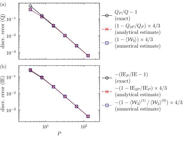
Figure 8: Comparison of exact analytical values of the path integral discretization error of (a) the partition function $Q$ and (b) isotope effect with their estimates [Eqs. (47) and (54)], which were evaluated either analytically or numerically using the estimator (52). The figure shows the dependence of the discretization error on the Trotter number $P$ in a one-dimensional harmonic oscillator with $\beta\hbar\omega=8$, and the isotope effect corresponds to the doubling of the mass.

Finally, note that expressions analogous to Eqs. (52) and (53) can also be derived for the fourth-order Takahashi-ImadaTakahashi and Imada (1984) and Suzuki-ChinSuzuki (1995); Chin (1997) factorizations. One needs to be careful, however, since both fourth-order factorization replace $V$ with an effective potential $V_{\text{eff}}$ that, unlike $V$, depends on $P$. As for the Suzuki-Chin factorization, the matter is further complicated by the fact that the weight of this effective potential depends on the bead $s$ at which it is evaluated.