Analysis of the dissipative range of the energy spectrum in grid turbulence and in direct numerical simulations

Abstract

We present a statistical analysis of the behavior of the kinetic energy spectrum in the dissipative range of fully developed three-dimensional turbulence, with the aim of testing a recent prediction obtained from the non-perturbative renormalization group. Analyzing spectra recorded in experiments of grid turbulence, generated in the Modane wind tunnel, and spectra obtained from high-resolution direct numerical simulations of the forced Navier-Stokes equation, we observe that the spectra decay as a stretched exponential in the dissipative range. The theory predicts a stretching exponent $\alpha=2/3$, and the data analyses of the numerical and experimental spectra are in close agreement with this value. This result also corroborates previous DNS studies which found that the spectrum in the near-dissipative range is best modeled by a stretched exponential with $\alpha<1$.

I Introduction

The very chaotic nature of the motion of a fluid driven to a turbulent state calls for a statistical description. A striking feature of turbulence is the emergence of very robust universal statistical properties, such as the well-known $k^{-5/3}$ decay of the energy spectrum over a wide range of length scales called the inertial range. This inertial range exists at sufficiently high Reynolds numbers, when the typical scale at which energy is injected (called the integral scale $L$) and the microscopic scale (called the Kolmogorov scale $\eta$) at which it is dissipated by molecular friction, are well separated.

The first understanding of these properties was provided by the pioneering statistical theory of turbulence proposed by Kolmogorov, and referred to as K41 Kolmogorov41a ; Kolmogorov91a ; Kolmogorov41c ; Kolmogorov91b . K41 theory relies on the fundamental assumptions that the small-scale turbulence is statistically independent of the large scales, that it is locally homogeneous, isotropic and steady, and that the average energy dissipation rate per unit mass $\epsilon$ is finite and independent of the kinematic viscosity $\nu$ in the limit $\nu\to 0$. This implies that the statistical properties of small-scale turbulence should be determined uniquely by $\epsilon$ and $\nu$. In particular, the energy spectrum should take the universal from

$$E(k)=\epsilon^{2/3}k^{-5/3}f(k\eta)$$ (1)

where $\eta=\nu^{3/4}\epsilon^{-1/4}$ is the Kolmogorov length scale. The function $f$ is universal. In the inertial range, viscous effects are expected to be negligible, so that the spectrum should not depend on $\eta$, which implies that $f(x)$ should tend to a constant $C_{K}$ for $x\to 0$, while $f$ should fastly decay at large wave-numbers $x\gtrsim 1$, which corresponds to the dissipative regime Kraichnan59 .

Although $f$ is expected to be universal, its analytical expression is not known. Several early empirical expressions of the form $f(x)\sim x^{-\beta}\exp(-\mu x^{\alpha})$, with different values for $\alpha$ (1/2 Tatarskii67 , 3/2 Uberoi69 , 4/3 Pao65 or 2 Townsend51b ; Novikov61 ; Gurvich67 ) were proposed, on the basis of approximate fits of experimental data or (approximate) analytical considerations Monin73 . Besides, different theoretical arguments focusing on the limit of large $k$ (Direct Interaction Approximation Kraichnan59 , asymptotic expansions Foias90 ; Sirovich94 ; Lohse95 ) advocated that in this limit, i.e. sufficiently deep in the far-dissipative range, the spectrum should decay as a pure exponential $\alpha=1$. Alternatively, the multi-fractal formalism predicts a universal form of the spectrum involving the Reynolds number Frisch91 .

Subsequently, the behavior of the spectrum in the dissipative range has been extensively studied in experiments Sreenivasan85 ; Smith91 ; She93 ; Saddoughi94 and Sanada92 ; Chen93 ; Martinez97 ; Ishihara05 ; Schumacher07 ; Ishihara09 ; Verma18 . Accurate experimental measurements of the spectrum at small scales are difficult to obtain, and several fits of the spectrum in the dissipative range have been proposed, for instance pure exponential functions with $\alpha=1$ but on two successive separate ranges in Sreenivasan85 , or a single pure exponential but with different coefficients $\mu$ in Saddoughi94 and Manley92 . Conversely, the analysis of Ref. Smith91 concluded that an exponential with $\alpha=2$ was the best fit for the experimental data, while still another empirical form is proposed in Pope00 .

The can in principle provide more accurate data for the spectrum in the dissipative range, but their high computational cost limits the studies to either low or moderate Reynolds numbers in order to reach high spectral resolution Chen93 ; Martinez97 ; Schumacher07 ; Verma18 or to lower spectral resolutions to reach higher Reynolds numbers Sanada92 ; Ishihara05 ; Ishihara09 . In practice, most of these works assumed that $\alpha=1$, and aimed at determining the exponent $\beta$ for the power laws (or combination of power laws) in front and the value of $\mu$. Although a pure exponential fit was shown to be a reliable model for the spectrum at very low Reynolds numbers Verma18 , it turned out not to be suitable to model the whole dissipative range already at moderate Reynolds numbers Martinez97 , and the result of the fit was found to depend significantly on the choice of the fitting range Ishihara05 .

An extended analysis of the existing results for the dissipative range is provided in a recent account Khurshid18 . This work (and previous studies) point to the conclusion that there exist two distinct regimes: the near-dissipative range (NDR) for $0.2\lesssim k\eta\lesssim 4$ and the far-dissipative range (FDR) for $k\eta\gtrsim 4$. In the NDR, the logarithmic derivative of the spectrum is not linear, such that a pure exponential is not a consistent description, and its curvature indicates that $\alpha<1$. In the FDR, the decay of the spectrum is well described by an exponential ($\alpha=1$). This finding explains the failure of previous attempts to describe the whole dissipative range as a pure exponential with various power-laws. The authors of Ref. Khurshid18 proposed a phenomenological modeling as a superposition of two exponentials, one with $\alpha<1$ dominating in the NDR and one with $\alpha>1$ dominating in the FDR. Note that no consensus seems to be reached concerning the power-laws multiplying the exponentials in either regimes.

Independently, a theoretical prediction for the behavior of the spectrum in the dissipative range has been recently obtained from a approach. This theoretical approach is a “first-principles” one, in the sense that it is based on the Navier-Stokes equation, without involving any phenomenological inputs nor uncontrolled approximations. It has recently led to a progress in the understanding of homogeneous isotropic and stationary turbulence, by providing the time dependence of multi-point correlation functions in the turbulent state Tarpin18 ; Tarpin19 . Concerning the energy spectrum, the NPRG yields a stretched exponential behavior with $\alpha=2/3$ in the NDR, and a regular one (pure exponential) in the FDR. This prediction provides a theoretical justification for the two-exponential phenomenological model proposed in Khurshid18 . This value for $\alpha$ in the NDR was then confirmed in Canet17 , and also in experiments of von Kármán turbulent swirling flow Debue18 . However, obtaining a quantitative estimate of the exponent of the stretched exponential is a difficult task, as it requires a sufficiently extended dissipative range and a high resolution.

In this work, we perform with a different compromise compared to previous studies favoring higher Reynolds numbers while keeping a sufficient spectral resolution in the NDR in order to reliably probe this regime. Moreover, we present a statistical analysis of the experimental data recorded in the Modane wind tunnel, featuring grid turbulence. Grid turbulence appears as a particularly suitable set-up to investigate the dissipative range, since high Reynolds numbers can be attained, and the Kolmogorov scale is typically larger in the air than in liquids, such that a higher resolution can be expected. Besides, the unique dimensions of the S1MA wind tunnel of ONERA in Modane, where the experiments discussed here were performed, allow one to investigate relatively high Reynolds number regimes with yet experimentally well resolved dissipative scales Bourgoin17 . In the following, we focus on the NDR, and more specifically on the exponential part, irrespective of the power-laws. We find from our analysis that the energy spectrum follows the predicted stretched exponential behavior, with an estimated exponent $\alpha=0.68\pm 0.19$, in close agreement with the NPRG result.

The remainder of the paper is organized as follows: in Sec. II, we give some details on the prediction. We present in Sec. III the results from the , and in Sec. IV the statistical analysis of the experimental data. Additional details are reported in the Appendices.

II Theoretical predictions from the non-perturbative Renormalization Group

We present in this section the principle of the and the main ideas underlying the derivation of Eq. (6) for the spectrum in the dissipative range, which we aim at testing. The purpose of this section is not to give technical details on its derivation, which can be found in Refs. Canet17 ; Tarpin18 , but rather to emphasize the underlying assumptions: it is based on the stochastic Navier-Stokes equation, and on an expansion at large wave-numbers, which leading term can be calculated exactly without any further approximations. One may resume directly at Eq. (4) for the result relevant for this work.

The idea of applying to turbulence Dominicis79 ; Fournier83 ; Smith98 ; Adzhemyan99 ; Zhou10 originates in the observation that the statistical properties of a turbulent flow are universal and described by power-laws in the inertial range. These power-laws are the hallmarks of scale invariance. The source of scale invariance at a critical point is the emergence of fluctuations at all scales. The , as originally conceived by Wilson Wilson74 , is a method to efficiently average over these (non-Gaussian) fluctuations to obtain the critical properties of the system. It should thus provide a valuable tool to study fully developed turbulence, which intrinsically involves length scales over many orders of magnitude.

The is a modern formulation, both functional and non-perturbative, of the Wilsonian , which turned out to be powerful to compute the properties of strongly correlated systems in high-energy physics, condensed matter and statistical physics Berges02 ; Kopietz10 ; Delamotte12 . It is only recently that turbulence has been revisited using functional and non-perturbative approaches Tomassini97 ; Monasterio12 ; Canet16 ; Tarpin18 ; Tarpin19 . Exact results were obtained in this framework for the time dependence of multi-point correlation functions of the stationary turbulent flow in the limit of large wave-numbers Tarpin18 ; Tarpin19 . These results hence pave the way towards a deeper understanding of the fundamental properties of turbulence.

The starting point is the forced equation for incompressible flows

$$\partial_{t}\vec{v}+\vec{v}\cdot\vec{\nabla}\vec{v}=-\frac{1}{\rho}\vec{\nabla}p+\nu\nabla^{2}\vec{v}+\vec{f}\,\,,\quad\vec{\nabla}\cdot\vec{v}=0\,$$ (2)

where $\nu$ is the kinematic viscosity and $\rho$ the density of the fluid. We are interested in universal properties of turbulence. These properties are expected not to depend in particular on the precise form of the forcing mechanism. We hence consider, as common in field-theoretical approaches Adzhemyan99 , a stochastic forcing, which has a Gaussian distribution with zero mean and variance

$$\langle f_{i}(t,\vec{x})f_{j}(t^{\prime},\vec{x}\,^{\prime})\rangle=\delta(t-t^{\prime})N_{L^{\text{-}1},{ij}}(|\vec{x}-\vec{x}\,^{\prime}|)\,,$$ (3)

where $\langle\cdot\rangle$ denotes the ensemble average over the realizations of $f$. This correlator is local in time, to preserve Galilean invariance, and is concentrated, in Fourier space, on the inverse of the integral scale $L$. The stochastically forced equation (2) can then be represented as a field theory following the standard Martin-Siggia-Rose-Janssen-de Dominicis (MSRJD) response functional formalism (Martin73, ; Janssen76, ; Dominicis76, ), which by essence includes all the fluctuations. In the treatment, the integration of these fluctuations is achieved progressively in the wave-number space, and yield a renormalization flow. Any $n$-point correlation function $G^{(n)}$ between velocity or pressure fields can be simply expressed in the field theory from the cumulant generating functional and obeys an exact flow equation. However, the flow equation for $G^{(n)}$ involves $G^{(n+1)}$ and $G^{(n+2)}$ which results in a infinite hierarchy of flow equations that needs to be solved.

It was realized in Canet16 ; Tarpin18 that these flow equations can be closed exactly in the limit of large wave-numbers using the symmetries of the field theory (or more precisely extended symmetries). Indeed, symmetries play a key role in field theory in general, since they yield exact relations between correlation functions known as (Ward identities). It turns out that the field theory possesses two extended symmetries, the time-dependent Galilean symmetry and a time-dependent shift symmetry recently unveiled Canet15 , which can be exploited to achieve the exact closure of the hierarchy of flow equations at large wave-numbers. Moreover, these flow equations can be solved analytically at the fixed point, which corresponds to the stationary turbulent state. Let us now give the result for the (transverse part of the) velocity-velocity correlation function $C$ defined as

$$C(t,{\vec{k}})\equiv\mathrm{TF}\left\langle{\vec{v}(t_{0}+t,\vec{x}_{0}+\vec{x})\cdot\vec{v}(t_{0},\vec{x}_{0})}\right\rangle,\\$$ (4)

$\mathrm{TF}$ denoting the Fourier transform with respect to $\vec{x}$. At small time lag $t$, $C(t,\,{\vec{k}})$ takes the form

$$C(t,\,{\vec{k}})=A\epsilon^{2/3}k^{-11/3}\exp\big{(}-\gamma(\epsilon L)^{2/3}(tk)^{2}+{\cal O}(k)\big{)},$$ (5)

where $\gamma$ and $A$ are non-universal constants Tarpin18 , $\epsilon$ is the mean energy dissipation rate and $L$ the integral scale. The leading term in $k^{2}$ in the exponential is exact, whereas the factor in front of the exponential is not. Indeed, the exponent of the power-law could be modified by terms of order $\ln(k)$ in the exponential, entering in the indicated ${\cal O}(k)$ corrections. The leading behaviour of the correlation function at large wave-numbers is hence a Gaussian in the variable $tk$, which is not the expected scaling variable. Indeed, dimensional analysis (Kolmogorov theory) predicts a dynamical critical exponent $z=2/3$ and thus a scaling variable $tk^{z}=tk^{2/3}$. The dependence in $tk$ is thus a breaking of standard scale invariance, generated by intermittency, it induces an explicit dependence in the integral scale $L$. An effective value $z=1$ for the dynamical exponent is a large correction. This effect is often described phenomenologically as the random sweeping effect Kraichnan59 ; Tennekes75 .

The energy spectrum can be described in the dissipative range by taking the appropriate $t\to 0$ limit Canet17 . One can assume that the scaling variable $tk^{2/3}$ saturates when $t$ approaches the Kolmogorov time-scale $\tau_{K}=\sqrt{\nu/\epsilon}$ and $k$ reaches $L^{-1}$, since these are the two relevant scales, such that $tk^{2/3}\to\tau_{K}L^{-2/3}$. One thus obtains for the energy spectrum $E(k)\equiv\lim_{t\to 0}4\pi k^{2}C(t,k)$ the expression

$$E(k)=A^{\prime}\,\epsilon^{2/3}(k\eta)^{-\beta}\exp\left(-\mu(k\eta)^{\alpha}\right),$$ (6)

where $\beta=5/3$, $\alpha=2/3$, $\mu$ and $A^{\prime}$ are positive non-universal constants related to $\gamma$ and $A$ respectively. This behavior is valid at large wave-numbers that are still controlled by the fixed point, it should correspond to the NDR. Indeed, in the FDR, for very small spatial scales, the spectrum should be regularized by the viscosity and should be analytical in real space, which means that it should decay as a pure exponential in $k$-space. The unusual emergence of a stretched exponential behavior is the manifestation of the violation of standard scale invariance. In standard scale invariance, there would be no transitional regime between the inertial regime and the FDR. The value $\alpha=2/3$ arises from the discrepancy between the Kolmogorov dynamical exponent and the effective one. Note that the emergence of this stretched exponential was also related in Ref. Khurshid18 to intermittency, and more precisely to intermittent energy transfers. It is indeed shown that the stretched exponential is removed by filtering out in time series of the energy spectrum the large intermittent bursts in energy at high wave-numbers.

The main purpose of this article is to attest the value of the exponent $\alpha$ in the exponential, and thereby to test the assumption of saturation of the scaling variable. Since the theory does not determine the prefactor of the exponential (as explained in our comment of (5)), we use a method which allows to estimate $\alpha$ irrespectively of the precise form of this prefactor, as follows. Extracting the value of $\alpha$ from the expression of the first logarithmic derivative of (6)

$$D_{1}(k\eta)=\frac{d\ln(E)}{d\ln(k\eta)}=-\beta-\mu\alpha(k\eta)^{\alpha}\,,$$ (7)

would require a three-parameter non-linear fit, which is not realistic given the typical extent of the NDR and quality of the data in this range. Previous works evidenced the high sensibility of such fits to the range of fitting or the initial condition of the fit algorithm Khurshid18 . Our analysis concentrates on the second and third logarithmic derivatives defined as

$$D_{2}(k\eta) =\frac{d(-D_{1})}{d\ln(k\eta)}=\mu\alpha^{2}(k\eta)^{\alpha}$$ (8)

$$D_{3}(k\eta) =\frac{d\ln(D_{2})}{d\ln(k\eta)}=\alpha\,.$$ (9)

In a log-log scale, the curve of $D_{2}$ in the dissipative range is expected to be a line with slope $\alpha$, while the curve of $D_{3}$ is expected to exhibit a plateau in this range of height $\alpha$. Beyond reducing the number of fit parameters, the main advantage of $D_{2}$ and $D_{3}$ is to provide a method to eliminate the contributions from sub-leading terms in the exponential of Eq. (5). Let us note that previous works predicted the existence of an energy pileup, called the bottleneck effect, leading to a bump of the compensated spectrum in the transitional regime between the IR and the NDR Falkovich94c ; Lohse95 . At the theoretical level, this effect modifies the prefactor of the exponential, which we do not try to resolve here. The numerical and experimental spectra we have analyzed do not show any noticeable bottleneck effect. However, it plays no role in the following analysis since it is eliminated in the higher derivatives $D_{2}$ and $D_{3}$ studied here. In the following, we first analyze the spectra obtained from in the dissipative range, and then present the analysis of the experimental data.

III Numerical data

III.1 Numerical simulations

We obtain the numerical energy spectra from of the NS equation under fully random large scale forcing and in isotropic and homogeneous conditions. The turbulent flow is simulated in a cubic periodic domain of size $2\pi$ with the same resolution in each of the coordinate directions. The Navier-Stokes equation is solved with the use of a pseudospectral parallelized code; time advancement is implemented with the second-order Runge-Kutta scheme Lagaert14 . The simulation parameters are determined by the and the value of $k_{\rm max}\eta$, where $k_{\rm max}$ is the maximal wave-number resolved in the spectrum. We perform a sequence of simulations with fixed and increasing grid resolution. In the first run the computational grid size is chosen to ensure at least $k_{\rm max}\eta=1.5$ which is commonly accepted as an adequate spatial resolution for . In the following runs the solution obtained in previous steps is transferred to a finer computational grid with resolution $N\rightarrow 2N$, while the $\Relam$ and the forcing scales are unchanged. By doing so, we increase twofold the value of $k_{\rm max}\eta$ and we therefore get access to smaller scales in the dissipative range of the turbulence spectrum. The values of the Taylor Reynolds number, size of the computational grid and associated value of $k_{\rm max}\eta$ used in the simulations are summarized in Tab. 1.

	60	90	160	240
256	3.0	1.5	-	-
512	6.0	3.0	1.5	-
1024	12.0	6.0	3.0	1.5
2048	-	12.0	6.0	3.0

Table 1: Parameters of the simulations: Maximal wave-number $k_{\rm max}\eta$ as a function of the Taylor microscale Reynolds number and the grid resolution $N$.

The spectra obtained for each $\Relam$ and resolution, averaged over space and time once the stationary state is reached, are displayed in Fig. 1, They exhibit an inertial range extending from about half a decade at $\Relam=60$ to about a decade and a half at $\Relam=240$. In this range, the spectra decay as power-laws with an exponent $K$ depending on the . These values are represented on Fig. 4, together with the experimental results. Both results are in agreement. Clearly, the determination of the exponent $K$ from the DNS spectra is not very precise, as the is limited, compared to standard with $k_{\rm max}\eta\simeq 1.5$. Let us recall that in this work we have chosen to favour the resolution over the extend of the inertial range, in order to increase the accuracy on the determination of $\alpha$. However, compared to previous works focused on the dissipation range, we choose a somewhat lower resolution (but still sufficient to resolve the NDR) while reaching a higher $\Relam$ Khurshid18 .

The first logarithmic derivatives $D_{1}$, defined by (7), of the DNS spectra is shown in Fig. 2. Their behavior is very similar to the ones obtained in previous works Martinez97 ; Ishihara05 ; Khurshid18 . In particular, one distinguishes two qualitatively different regimes: the NDR up to $k\eta\approx 4$, and the FDR extending beyond this value. In the NDR, the $D_{1}$ curves exhibit a slight convex curvature, more visible as the $\Relam$ increases, which indicates that $\alpha<1$ in this region. In the FDR, the curves of $D_{1}$ appear reasonably linear in log-log scale, indicating a pure exponential decay $\alpha\simeq 1$. Moreover, the curves do not collapse in this range, suggesting that this regime is not universal. These observations are in good agreement with previous studies, and lead in particular to the two-exponential model of Ref. Khurshid18 , one with $\alpha<1$ dominant in the NDR, and the other one with $\alpha=1$ in the FDR.

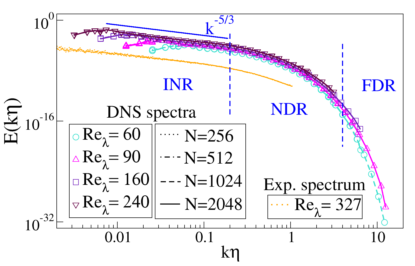
Figure 1: Spectra obtained from , for the set of and resolutions $N$ given in Tab. 1. In all the figures, INR, NDR and FDR stand for inertial range, near-dissipative range and far-dissipative range respectively.

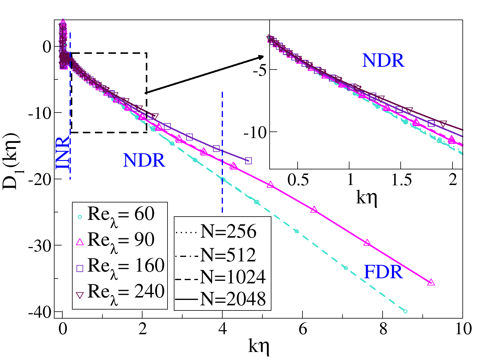
Figure 2: First logarithmic derivative $D_{1}$ of the spectra of Fig. 1, with the inset showing a zoom in the near-dissipative range. These results are very similar to those obtained in previous works Martinez97 ; Ishihara05 ; Khurshid18 . In particular, $D_{1}$ is not linear in the NDR, hence it is not compatible in this range with a pure exponential behaviour ($\alpha=1$).

III.2 Analysis of the numerical spectra in the near-dissipative range

In order to push further the previous observations, and to obtain a precise determination of the exponent $\alpha$ in the NDR,

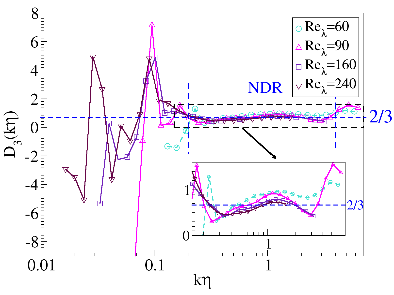
Figure 3: Third logarithmic derivative, defined by (9), computed for the spectra of Fig. 1, with the inset showing a zoom in the near-dissipative range. Only the curves for the highest resolution for each $\Relam$ are shown for clarity. They all show a plateau in the NDR, whose value is $\alpha$, which approaches 2/3 as the increases.

we compute the second and third logarithmic derivatives defined by (8) and (9) for the spectra of Fig. 1. Our numerical data are smooth enough to allow for the numerical evaluation of the successive derivatives by finite differences.

The result for the third derivative is displayed on Fig. 3, for the different $\Relam$’s. The results for the second derivative show very similar features. The $D_{3}$ curves clearly exhibit a plateau for values of $k\eta$ in the NDR, in agreement with the theoretical expression (9). The value of this plateau is smaller than 1, and appears to be very close to the NPRG prediction $\alpha=2/3$. The inset is a magnification of the plateau, which shows that $\alpha$ is close to one at small and approaches the value $\alpha=2/3$ as the $\Relam$ grows. This is in excellent agreement with Ref. Khurshid18 , where they find a value of $\alpha$ in the NDR decreasing as $\Relam$ increases, down to $\alpha\simeq 0.78$ for their highest $\Relam=89$ (we find $\alpha\simeq 0.77$ for $\Relam=90$, see Fig. 5).

The average value of $\alpha$ on the plateau is represented in Fig. 5 as a function of the , together with the experimental results. Both results are in agreement. The extent of the NDR seems to remain $0.2\lesssim k\eta\lesssim 4$ independently of the $\Relam$. Interestingly, one observes that, for the spectra at lower , $D_{3}$ departs from the plateau at higher wave-numbers – in the FDR, towards a value which we anticipated as  $1$, which would signal the setting of the regular (simple exponential) behavior. However, the expected value $\alpha=1$ cannot be quite reached in the because of the truncation of wave-numbers at a finite $k_{\rm max}$.

The analysis of the numerical spectra is thus in quantitative agreement with the theoretical prediction $\alpha=2/3$, and provides useful indications to guide the analysis of the experimental data.

IV Experimental data

IV.1 Data pre-processing

Let us describe the experimental data of grid turbulence acquired in the S1MA wind tunnel at Modane (ESWIRP project). The data are made of velocity time-series recorded by four hot wires at a frequency of 250 kHz, with durations ranging from 3 to 10 minutes each. The turbulent flow source blows air at speed ranging from 20m.s^-1 to 45m.s^-1, resulting in a variety of values for $\Relam$. The distance of the hot wires from the grid ranges from 7.9m to 23.16m Bourgoin17 . We analyze all the recordings using a systematic procedure described below, focusing on the energy spectra.

We divide the recordings into samples of equal time duration $\Delta t=20$s (respectively $\Delta t=60$s). This provides us with a total number of 3840 (respectively 1176) samples, which we analyze separately. We use the Taylor hypothesis to express the velocity as a function of the longitudinal space coordinate. For each sample, we compute the third-order structure function $S_{3}(\ell)=\langle(\delta u_{\ell})^{3}\rangle$ where $\delta u_{\ell}$ is the longitudinal velocity increment $\delta u_{\ell}=\big{(}\vec{u}(\vec{r}+\vec{\ell})-\vec{u}(\vec{r})\big{)}\cdot\vec{\ell}/|\vec{\ell}|$. We determine the corresponding average injection/dissipation rate per unit mass $\epsilon$ from the plateau value of $S_{3}$ using the four-fifth law: $\epsilon=-\frac{5}{4}S_{3}(\ell)/\ell$ in the inertial range. We then compute the associated Kolmogorov scale as $\eta=\nu^{3/4}\epsilon^{-1/4}$, with $\nu=1.5\times 10^{-5}\mathrm{m^{2}.s^{-1}}$ the air kinematic viscosity. The Taylor microscale Reynolds number for each sample is deduced using the isotropic relation $\mathrm{Re}_{\lambda}=u_{\rm rms}\sqrt{15/\nu\epsilon}$. Let us note that the determination of $\epsilon$ through the four-fifth law is not very precise, and thus it entails some error on the . However, we also used another determination of $\epsilon$, through the position of the peak of the dissipative spectrum $k^{2}E(k)$, and we checked that this does not change the different distributions shown here, nor the final value of $\alpha$.

We compute the kinetic energy spectrum of each sample by performing a discrete Fourier transform (FFT algorithm) and rescale it as a function of the dimensionless wave-number $k\eta$. (A typical spectrum is displayed at the top of the Fig. 10.) We smoothen the spectra out using a regular binning of 20,000 bins in $\ln(k\eta)$ scale. In the experimental spectra, $k\eta$ typically ranges from $10^{-3}$ to $3.5$. The quality and the extent in wave-number of the spectra vary quite substantially between the samples. The variability of the measurement quality comes from the fact that the wind tunnel is an open facility in which dust and pollen can enter and affect the hot wires. Because of this issue, some values of $\epsilon$ are questionable, which explains why some values of $\Relam$ are out of the range $200-600$. However, all of them appear to increase as functions of $k$ beyond a wave-number $k_{M}$, which we interpret as a contamination by the small-scale response of the hot wires. The value of $k_{M}$ depends on the spectra, but is found to be typically $k_{M}\eta\simeq 3$. In the following, we restrict the analysis to wave-numbers below $k_{M}$. Note that we do not observe any noticeable bottleneck effect on the experimental spectra analyzed. As this effect is expected to attenuate when the $\Relam$ increases Donzis10 , it would be difficult to detect here, moreover as already explained, it alters the prefactor of the exponential and disappears in the higher derivatives considered in the present work.

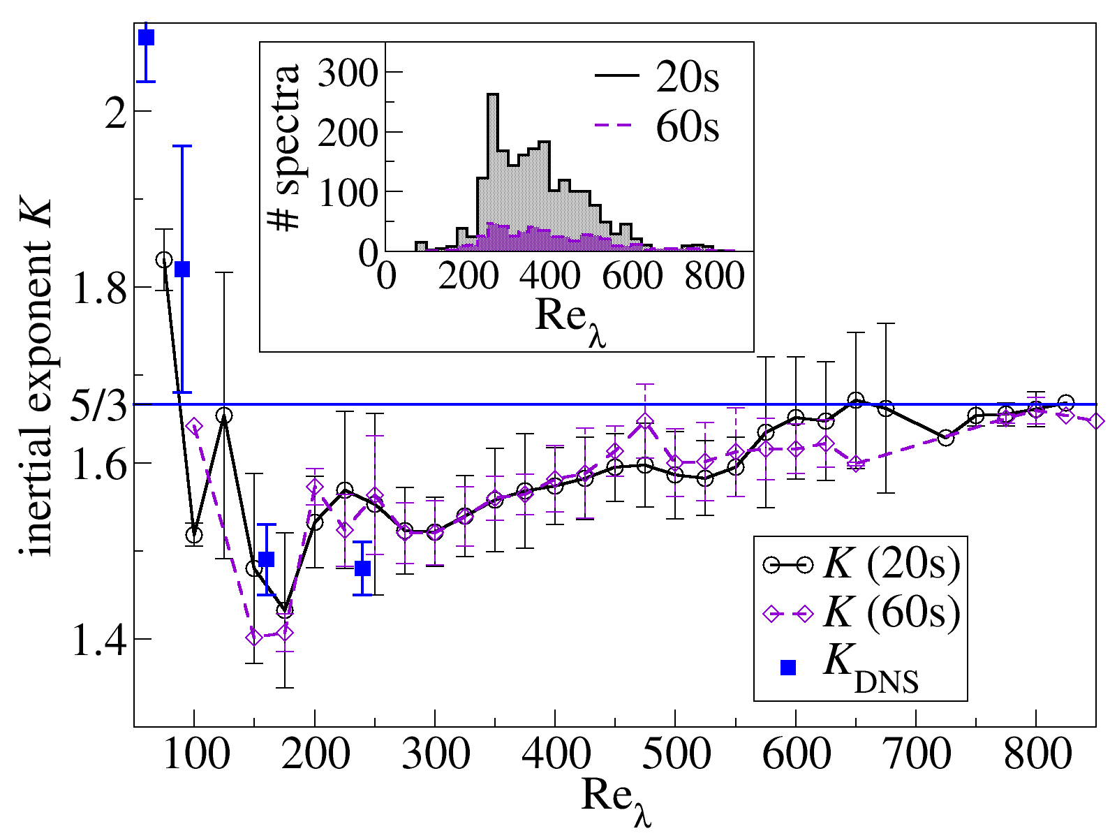
Figure 4: Exponent $K$ of the power-law in the inertial range, from and from experiments for both sample durations $\Delta t=20$s and $\Delta t=60$s, as a function of the Taylor microscale Reynolds number. For the experimental points, the symbols represent the mean values of $K$ on each $\Relam$ bin, and the error bars the standard deviation within each bin. The number of spectra in each bin is not equal, it is given by the distribution shown in the inset.

IV.2 Selection of spectra

In order to assess the quality of each sample and to remove low-quality spectra, we operate a data-driven selection, based on the value of the inertial range exponent $K$ and on the extent of the dissipative range, whose determinations are detailed in Sec. IV.3 and Sec. IV.4 respectively. We first eliminate for both sample durations $\Delta t=20$s or $\Delta t=60$s the spectra with an exponent $K$ differing from the K41 value by more than $20\%$. This procedure typically removes very noisy spectra presenting several unphysical large peaks. After this first filtering, there remain 3486 (respectively 1080) exploitable spectra for $\Delta t=20$s (respectively $\Delta t=60$s). We then proceed to a second selection by retaining only the spectra with a large enough dissipative range of width $\Delta(k\eta)>0.2$. This second selection removes spectra which are not well resolved in the dissipative range, probably affected by the noise from the sensor. This finally leaves us with 1641, respectively 590 spectra, for $\Delta t=20$s and $\Delta t=60$s. We only further analyze and discuss these selected spectra in the following.

IV.3 Inertial range

In this section, we briefly describe the analysis of the spectra in the inertial range. We determine the exponent $K$ of the power-law decay of the energy spectrum $E(k\eta)\sim(k\eta)^{-K}$ in this range, to be compared with the expected K41 value $K\simeq 5/3$. We do not denote it $\beta$ as in (6) since we do not assume the two exponents to be equal in the inertial and dissipative ranges. We use two methods to estimate $K$: a direct fit of the log-log spectrum – which is expected to be a line in the inertial range, and a fit of the first logarithmic derivative $D_{1}$ – which is expected to present a plateau of value $-K$ in the corresponding range. Throughout this work, we only use fitting functions which are affine (either lines or constants). The result of a fitting procedure is in general sensitive to the precise fitting interval chosen, and to the chosen precision criterion. In order to reduce as much as possible these effects, we devise an optimized algorithm, described in Appendix A, whose goal is to search for the largest interval with the minimal error where an affine behavior is present. For each spectrum, we apply this fitting algorithm to both the log-log spectrum and the corresponding $D_{1}$, and compare these two results, If the relative difference in the obtained $K$ is less than 2%, we take the average value. Otherwise we keep the estimate for $K$ which corresponds to the largest interval.

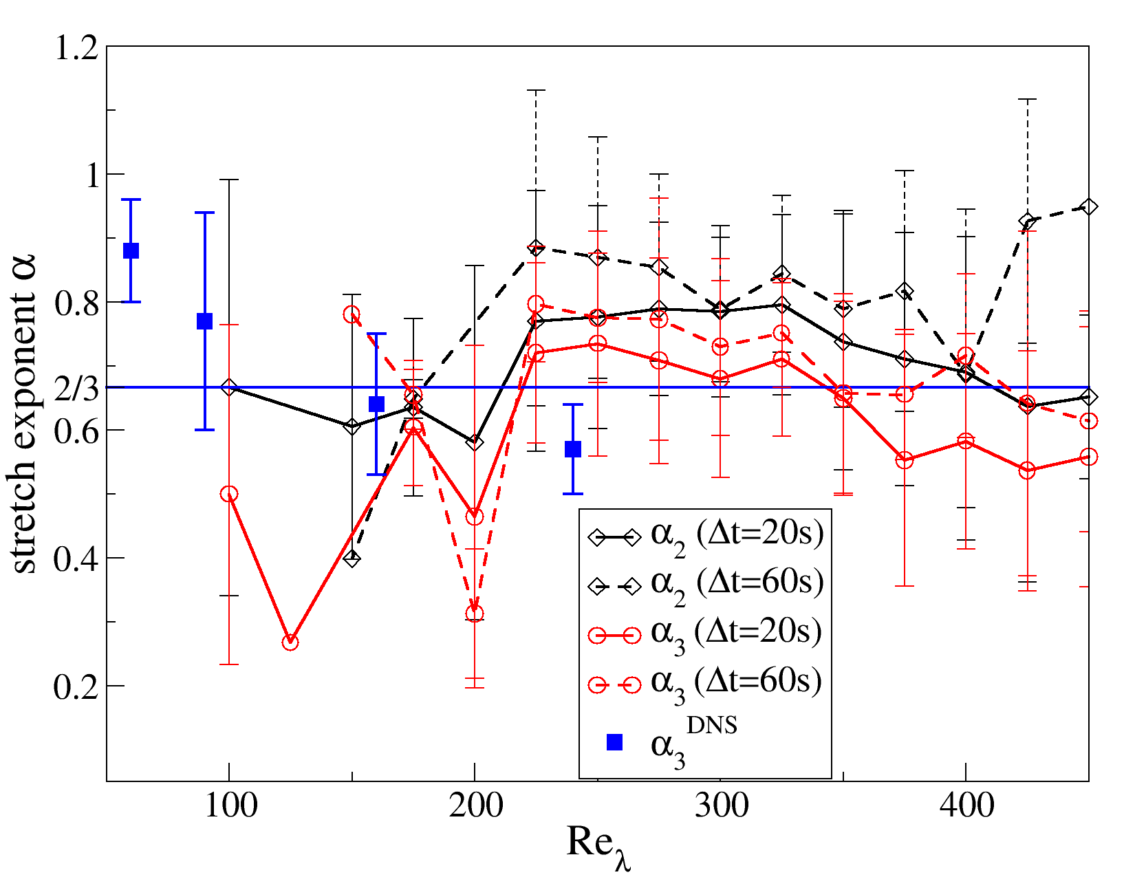
Figure 5: Stretch exponent $\alpha$ as a function of the Taylor microscale Reynolds number from and from experiments: $\alpha_{2}$ (black lines with diamonds) computed from $D_{2}$ and $\alpha_{3}$ (red lines with triangles) computed from $D_{3}$, for experimental spectra corresponding to both duration $\Delta t=20s$ (plain lines) and $\Delta t=60s$ (dashed lines), and $\alpha_{3}$ (blue squares) from . For the experimental points, the symbols indicate the mean values of $\alpha$ for each $\Relam$ bin, and the error bars the standard deviation within each bin. The number of spectra in each bin is not equal, the distribution of $\Relam$ for each set of spectra is represented in Fig. 6.

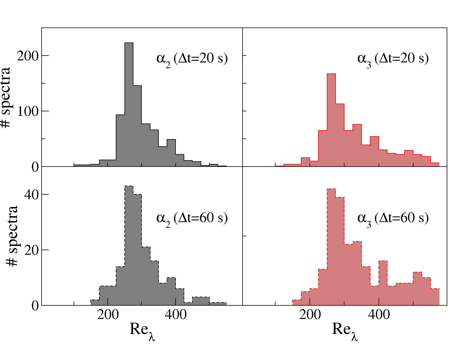
Figure 6: Distribution of the $\Relam$ corresponding to each set of data displayed in Fig. 5, for the two sample durations $\Delta t=20s$ and $\Delta t=60s$, and for the two methods $D_{2}$ and $D_{3}$.

We present in Fig. 4 the results for the exponent $K$ as a function of the , for the two sample durations $\Delta t=20$s and $\Delta t=60$s. The experimental data correspond to distributed between 25 and 1150, among which more than $90\%$ lie between 150 and 650. Their distribution is represented in the inset of Fig. 4, using bins of width $\Delta\Relam=25$, and computing within each bin the average and the standard deviation of the decay exponent $K$. The error bars in Fig. 4 represent the standard deviation within each bin, irrespective of the total number of spectra they contain. Note that the weight of the different points is thus very different: for instance the first points at low $\Relam$ represent very few spectra. We observe that the value of the inertial exponent $K$ grows with the $\Relam$, to reach a value close to $K=5/3$ for $\Relam\gtrsim 600$. The results for both durations are in close agreement. However, let us emphasize that this determination is not accurate enough to detect the corrections due to intermittency, which are expected to increase by about 5% the K41 value $K=5/3$. The error bars of the points around $\Relam=600$ obtained for the duration $20$s are typically representative since they correspond to a large number of spectra, and they clearly exceed the 5% level of tolerance needed to estimate intermittency corrections on the inertial range exponent.

IV.4 Near-dissipative range and stretch exponent

In this section, we turn to the analysis of the near-dissipative range. As for the data, we rely for the experimental data on two independent estimations of the stretch exponent $\alpha$: one from the second logarithmic derivative $D_{2}$ given by (8) and one from the third one $D_{3}$ given by (9). The experimental data are much less smooth than the numerical ones, such that performing simple finite differences to compute numerical derivatives generates a lot of noise, which would spoil the accuracy of this procedure. For this reason, we resort to a more reliable computation of the derivatives, described in Appendix A. We obtain two determinations of $\alpha$ denoted $\alpha_{2}$ and $\alpha_{3}$, from the optimized linear fitting of $D_{2}$ in log-log scale, and from applying to $D_{3}$ the same optimized algorithm to search for a plateau respectively. We only retain estimations of $\alpha$ for which the error of the associated fit is less than $Q=10^{-1}$ (see Appendix A for the definition of $Q$).

We present on Fig. 5 the results obtained for $\alpha_{2}$ and $\alpha_{3}$ as functions of the $\Relam$, for both sample durations $\Delta t=20$s and $\Delta t=60$s. The distribution of $\Relam$ corresponding to the four sets of spectra are displayed in Fig. 6. The large majority of spectra presents a $\Relam$ again lying in the range $200\lesssim\Relam\lesssim 500$. The number of spectra with a $\Relam$ outside this range is negligible. Contrary to the inertial exponent $K$, we do not observe for $\alpha$ a clear dependence on the $\Relam$ (at least not within the present level of accuracy), but rather a constant value (up to fluctuations) smaller than 1. The error bars on Fig. 5 represents the standard deviation within each $\Relam$ bin, and do not reflect the fact that some bins (at lower or larger $\Relam$) contain very few spectra. Moreover, one notices that the estimation of $\alpha_{2}$ appears systematically larger than the one from $\alpha_{3}$. The determination of $\alpha_{2}$ involves a two-parameter fit, such that the resulting value for $\alpha_{2}$ is expected to be less precise than the one of $\alpha_{3}$, but we have no interpretation for the seemingly systematic over-estimation.

Since we did not find any sizeable dependence of the stretch exponent $\alpha$ on the $\Relam$, we rather concentrate in the following on the distributions of the values of $\alpha$. We present in Fig. 7 these distributions for the same data as the one used in Fig. 5, that is both $\alpha_{2}$ and $\alpha_{3}$ and for both sample durations. One notices again that the distributions for $\alpha_{2}$ are slightly shifted upward with respect to the ones for $\alpha_{3}$. The averages and standard deviations of all the distributions are gathered in Tab. 2.

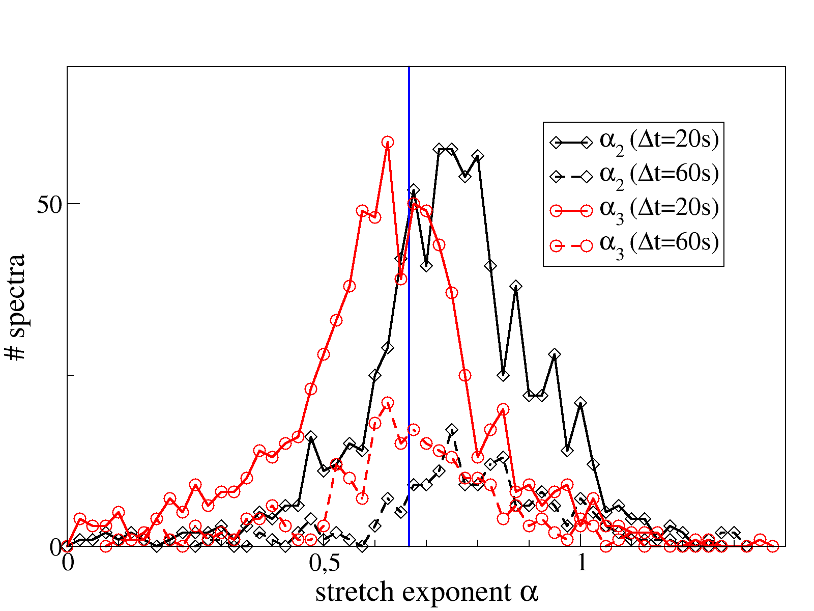
Figure 7: Distribution of the stretch exponent $\alpha$: $\alpha_{2}$ (black lines with diamonds) computed from $D_{2}$ and $\alpha_{3}$ (red lines with triangles) computed from $D_{3}$, for spectra corresponding to both durations $\Delta t=20s$ (plain lines) and $\Delta t=60s$ (dashed lines). The mean value and standard deviation of these distributions are reported in Table 2.

The distributions presented in Fig. 7 correspond to an error tolerance of $Q=10^{-2}$. We studied the influence of this precision criterion by varying it from $10^{-1}$ to $10^{-4}$. The corresponding distributions for $\alpha_{3}$ are displayed in Fig. 8. It is remarkable that the more stringent the precision criterion, the narrower the distributions around the theoretical prediction $\alpha=2/3$. In fact, very few spectra pass the highest precision criterion $Q=10^{-4}$ for the sample duration $\Delta t=60$s, and none for $\Delta t=20$s.

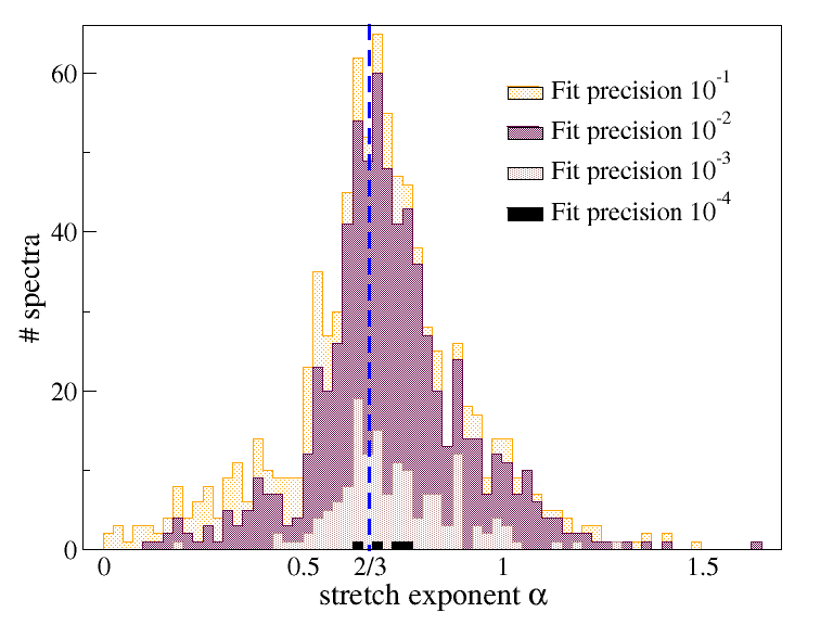
Figure 8: Distribution of the stretch exponent $\alpha_{3}$ for $\Delta=60$s and for different precision criteria $Q$ from $10^{-1}$ to $10^{-4}$.

To give a final number for $\alpha$, we can favor the most precise determination, which is $\alpha_{3}$. We retain the two precision criteria $Q=10^{-2}$ and $Q=10^{-3}$, which embody a reasonable compromise between the level of accuracy and the level of statistics. Finally, since the spectra for both sample durations constitute independent sets of comparable qualities, we can consider a weighted average of these results, which yields

$$\langle\alpha_{3}\rangle_{10^{-2}}\simeq 0.677\pm 0.193\quad,\quad\langle\alpha_{3}\rangle_{10^{-3}}\simeq 0.712\pm 0.157\,.$$

Both estimates are very close, since their one-$\sigma$ intervals are respectively $\alpha\in[0.48:0.87]$ and $\alpha\in[0.55:0.87]$. We hence choose as a representative final result

$$\langle\alpha\rangle\simeq 0.68\pm 0.19\,.$$

The present analysis indicates that values $\alpha<0.4$ or $\alpha>0.9$ can be reasonably excluded.

$\alpha_{i}$	$\Delta t$	$Q$	#	$\langle\alpha\rangle$	$\sigma$
$\alpha_{2}$	20s	$10^{-1}$	792	0.754	0.181
		$10^{-2}$	785	0.757	0.176
		$10^{-3}$	685	0.782	0.151
		$10^{-4}$	282	0.756	0.126
	60s	$10^{-1}$	178	0.805	0.188
		$10^{-2}$	175	0.812	0.178
		$10^{-3}$	162	0.833	0.159
		$10^{-4}$	99	0.829	0.126
$\alpha_{3}$	20s	$10^{-1}$	2892	0.621	0.226
		$10^{-2}$	1798	0.661	0.194
		$10^{-3}$	89	0.678	0.167
		$10^{-4}$	0	–	–
	60s	$10^{-1}$	878	0.690	0.224
		$10^{-2}$	703	0.719	0.190
		$10^{-3}$	153	0.730	0.151
		$10^{-4}$	4	0.710	0.052

Table 2: Summary of the number of spectra (#), average value ($\langle\alpha\rangle$) and standard deviation ($\sigma$) of the distributions of the stretch exponent $\alpha$ obtained from either the second ($\alpha_{2}$) or the third ($\alpha_{3}$) logarithmic derivatives, for spectra of both sample durations $\Delta t=20$s and $\Delta t=20$s, and for different precision tolerances $Q$ on the fit.

IV.5 Near-dissipative range: other parameters

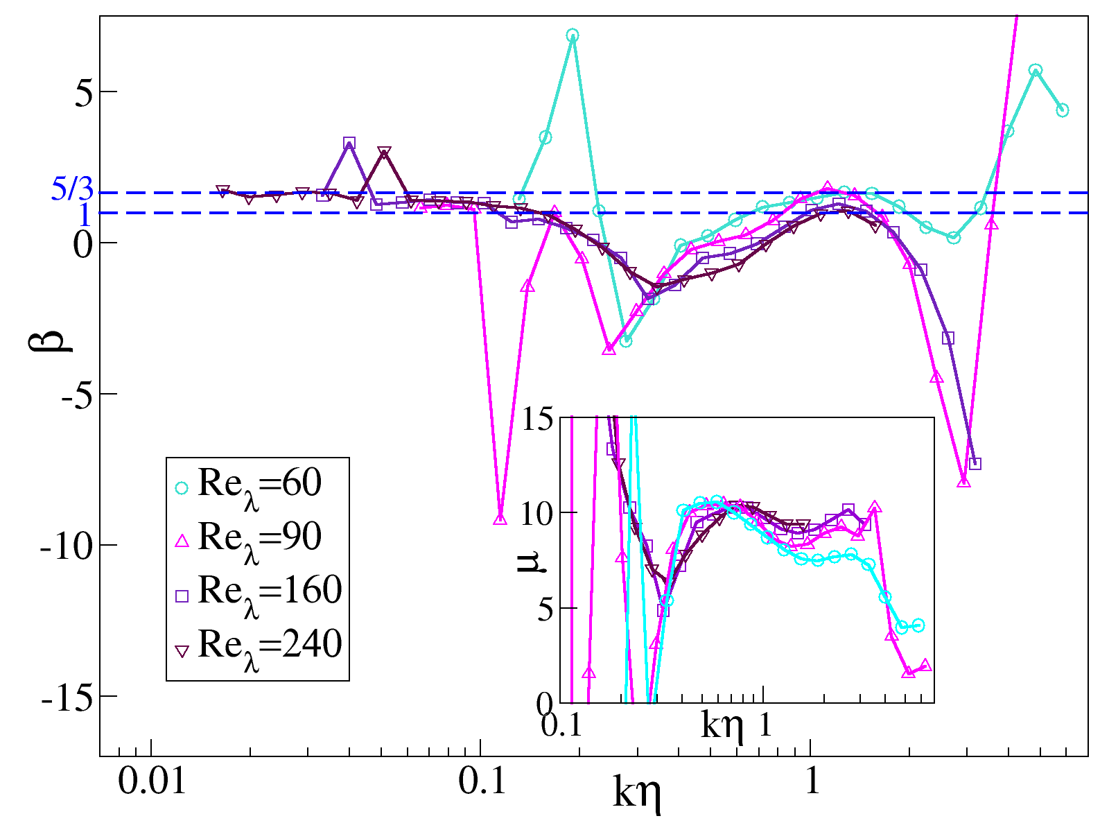
Figure 9: Parameters $\beta$ (main graph) and $\mu$ (inset) obtained for the spectra of Fig. 1.

For completeness, we also give in this section the results for the other parameters of (6): the multiplicative constant $\mu$ in the exponential, and the exponent $\beta$ of the power-law. The parameter $\mu$ can be obtained from the constant $\mu\alpha^{2}$ in the linear fit of $D_{2}$ in log-log scale according to (8). The values found for the experimental data are given in Tab. 3. If we consider, as we do for $\alpha$, the weighted average of both sample durations for $Q=10^{-2}$, we obtain:

$$\langle\mu\rangle\simeq 4.45\pm 1.31\,,$$

which turns out to be of the same order as values found in previous studies Debue18 , although $\mu$ is not expected to be universal. In the numerical data, we obtain somewhat higher values, of order 10, as shown in Fig. 9.

The value of $\beta$ can be computed as

$$\beta=\frac{D_{2}(k\eta)}{D_{3}(k\eta)}-D_{1}(k\eta)\,.$$ (10)

However, the precision on $\beta$ is very poor, and it is highly sensitive to the value found for $\alpha$. As an indication, we find in the experimental data values close to $1$, as summarized in Tab. 3. For instance for $Q=10^{-2}$, we obtain from the weighted average of both samples durations:

$$\langle\beta\rangle\simeq 0.93\pm 0.26\,.$$

In the , the value obtained for $\beta$ is shown in Fig. 9. It turns out to be close to $\beta=5/3$ i.e. to the inertial range value) at small $\Relam$, and to tend to a smaller value very close to $\beta=1$ as $\Relam$ increases, in agreement with the results from the experimental data. But once again, these estimates should be taken with caution. Given the typically small extent of the NDR, the determination of the leading behavior, through $\alpha$, is already challenging, such that a precise determination of the sub-leading one, through $\beta$, is beyond the reach of the present work.

$\Delta t$	$Q$	#	$\langle\mu\rangle$	$\sigma_{\mu}$	$\langle\beta\rangle$	$\sigma_{\beta}$
20s	$10^{-1}$	750	4.51	1.26	0.92	0.26
	$10^{-2}$	747	4.51	1.26	0.92	0.26
	$10^{-3}$	672	4.46	1.23	0.93	0.27
	$10^{-4}$	275	4.53	1.07	0.87	0.25
60s	$10^{-1}$	173	4.16	1.54	0.99	0.27
	$10^{-2}$	172	4.19	1.51	0.98	0.26
	$10^{-3}$	162	4.06	1.28	1.00	0.23
	$10^{-4}$	99	3.90	0.89	1.00	0.19

Table 3: Average value and standard deviation of the distributions of the parameters $\mu$ and $\beta$ obtained for spectra of both sample durations $\Delta t=20$s and $\Delta t=60$s, and for different precision tolerances $Q$ on the fit.

V Conclusion

In this work, we analyze the near-dissipative range of kinetic energy spectra obtained from high-resolution and from experimental grid turbulence in the Modane wind tunnel in order to test the prediction of a stretched exponential behavior $E\propto\exp(-\mu(k\eta)^{\alpha})$ with exponent $\alpha=2/3$ in this range. We use two independent determinations, from the second and from the third logarithmic derivatives of the spectra, to estimate the value of $\alpha$. All the results, from and from experiments, and from the different determinations, are consistent, and yield an estimate for the stretch exponent $\alpha\simeq 0.68\pm 0.19$, in full agreement with the theoretical prediction.

Let us emphasize that the typically small extent of the near-dissipative range and the level of precision currently accessible in or experimental data do not seem sufficient to reliably determine the prefactor of the exponential, that is the precise form of the power-laws. Hence, the present analysis does not allow us to shed a new light on this point. It could possibly be refined in the future if data with still higher resolution become available. Moreover, it would be also very interesting to further test the NPRG predictions concerning the time dependence of two- or multi-point correlation functions, in or in experiments which dispose of suitable measurement techniques.

Appendix A Numerical procedures

A.1 Optimized linear fitting algorithm

Extracting the inertial or dissipative exponents from the experimental data always amounts to an affine fit (either lines in log-log representation or constants). For this, we use an elementary linear regression. However, the accuracy of the result of such a fit strongly depends on the choice of the fitting domain $D$, which is delicate since there is no clear delimitation of the inertial or dissipative ranges. Let us denote by $a(D)$ and $b(D)$ the real numbers such that the standard linear fit in the domain $D$ is the affine function $x\mapsto f(x)=a(D)x+b(D)$ and by $x_{i}$ a data point in the domain $D$, i.e. $x_{i}\in D$, and $y_{i}=f(x_{i})$.

To determine the best fitting domain, we use an optimized method based on the alignment of data points in a given domain $D$. The alignment $\lambda(D)$ is the largest absolute deviation of a data point from the linear fit performed in this domain: $\lambda(D)=\max_{x_{i}\in D}|a(D)x_{i}+b(D)-y_{i}|$. Based on $\lambda(D)$, our algorithm seeks the largest domain $D(\varepsilon)$ such that $\lambda(D)<\varepsilon$ for any given positive number $\varepsilon$. $\varepsilon$ stands as a quality requirement of the input data. We estimate the quality $Q(D)$ of the result using the standard error $Q=\sigma/\sqrt{n}$ where $\sigma$ is the standard deviation and $n$ is the number of data points in the domain. Assembling these elements, we determine the value $\varepsilon_{\rm opt}$ that minimizes the function $Q(D(\varepsilon))$ and use $D(\varepsilon_{\rm opt})$ as the optimal domain. This procedure is used to determine the inertial exponent $K$ of the spectrum and the stretch exponent $\alpha$ from the second logarithmic derivative $D_{2}(k\eta)$.

We use the same procedure to find the optimal plateau, i.e. the optimal domain where the curve has the lowest slope. This is achieved by replacing $Q$ by $Q^{\prime}(D)=Q(D)+|a(D)|$, where $a(D)$ is as before the slope of the linear fit in the domain $D$. We use this method to determine the inertial exponent $K$ from the first logarithmic derivative $D_{1}(k\eta)$ and for the stretch exponent $\alpha_{3}$ from the third logarithmic derivative $D_{3}(k\eta)$. The value of $Q$ is recorded for each estimate, and is used as a precision indicator for the quality of the fit. In particular, we rely on $Q$ to set up different precision criterion, eg. in Fig. 8 or Tab. 2. The application of these procedures is illustrated in Sec. A.3 on a typical spectrum.

A.2 Numerical computation of derivatives for the experimental data

As explained in Sec. IV.4, the direct computation by finite differences of successive derivatives of the experimental spectra is too noisy to be exploitable. Instead, to smooth out the data, we use the following procedure. The derivative of a function at a certain point is computed by implementing a linear fit in a window $D$ centered around this point containing a fixed number of data points (we typically use windows of 50 points). The linear fit coefficient $a(D)$ is thus an estimate of the value of the derivative at this point. By sliding the window $D$ through all the data points, we obtain the derivative of the whole function. The logarithmic derivatives of the type $d\ln f/d\ln q$ are performed using the same method with a power law fit (fitting function $q\mapsto b(D)q^{a(D)}$) and the derivatives of the type $d/d\ln q$ with an exponential fit (fitting function $q\mapsto b(D){\mathrm{e}}^{a(D)q}$). With this procedure, the resulting derivatives of the experimental spectra are smooth enough to serve for further analysis.

A.3 Illustration of the determination of the exponents $K$ and $\alpha$

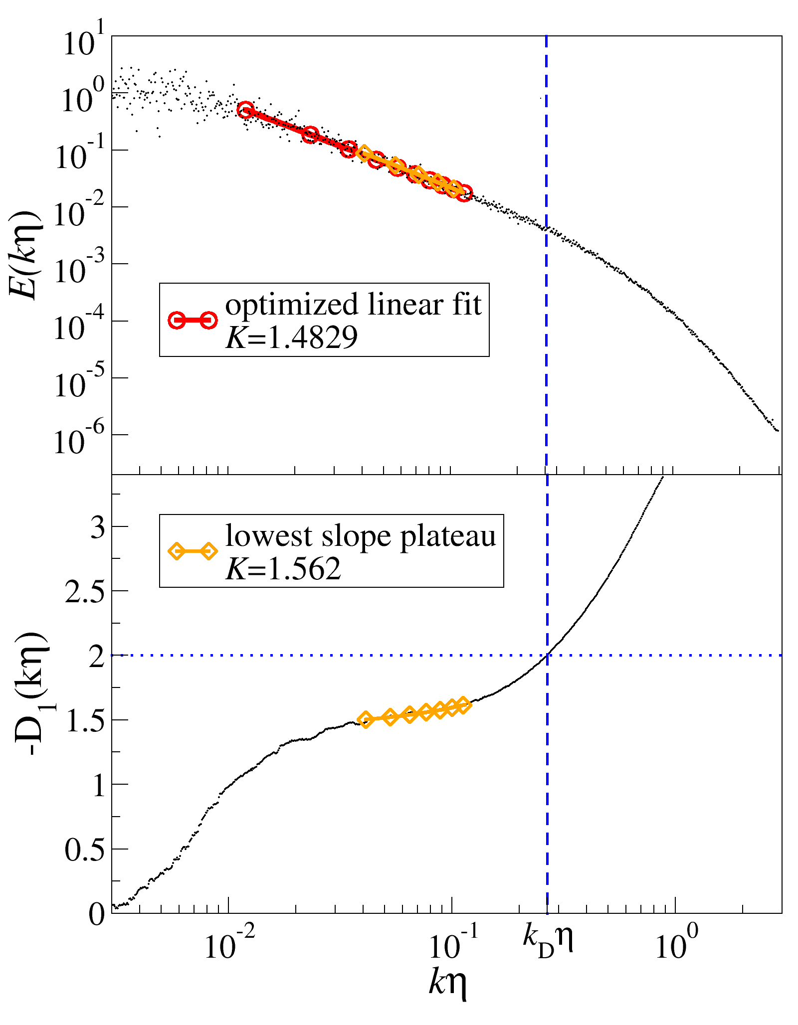
Figure 10: Result of the optimized fitting algorithm for the determination of $K$ from the log-log spectrum (red line with circles) and from the first logarithmic derivative $D_{1}$ (orange line with diamonds). The result from $D_{1}$ is reported on the spectrum $E$ for comparison.

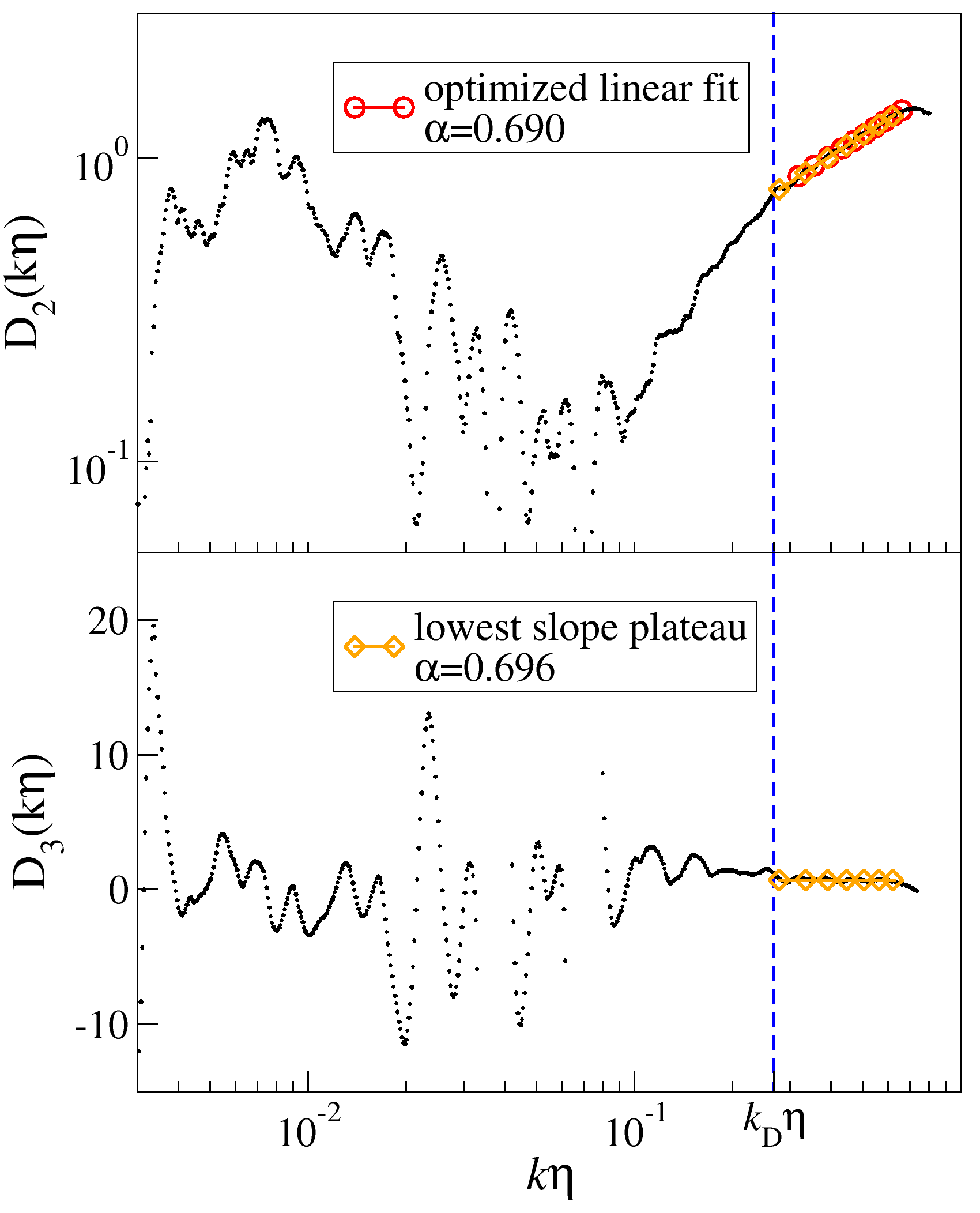
Figure 11: Result of the optimized fitting algorithm for the determination of $\alpha$ from the second (red line with circles) and from the third (orange line with diamonds) logarithmic derivatives of the spectrum. The result from $D_{3}$ is reported on the $D_{2}$ curve for comparison.

As an illustration of the procedures described above, we present their result on a typical spectrum. The determination of $K$ is illustrated in Fig. 10, which shows this particular spectrum $E(k\eta)$ in log-log scale and its first logarithmic derivative $D_{1}(k\eta)$, obtained as explained in the previous section. The $D_{1}$ curve is first used to estimate the dissipative wave-number $k_{\rm D}$, which we define as the wave-number for which $(k\eta)^{2}E(k\eta)$ is maximum, and hence corresponds to the value $D_{1}(k_{\rm D}\eta)=2$. We find $k_{\rm D}\eta\simeq 0.18$, which is in agreement with typical values in the literature and also with the value found for the numerical spectra. This value can be used as a reliable upper bound for the inertial range. The search for the largest best domain with linear behavior for $E$ and lowest slope plateau for $D_{1}$ is initialized in the range $k\eta\in[0.01,k_{\rm D}\eta]$. The result of the optimized algorithm is represented, with their respective domains, as the red line with circles and orange line with diamonds respectively. In this example, the two values for $K$ differ by more than 2% so the value from the linear fit of $E$ is retained since it corresponds to the largest domain.

The determination of $\alpha$ is illustrated in Fig. 11, which shows the second $D_{2}$ and third $D_{3}$ logarithmic derivatives defined in (8) and (9) respectively. The numerical derivatives are evaluated as described in the previous section. The search domain for the near-dissipative range is initialized as $k\eta\in[k_{\rm D}\eta,k_{M}\eta=3]$. The result of the optimized linear fitting algorithm applied to $D_{2}$ to extract $\alpha_{2}$ (and $\mu\alpha_{2}^{2}$ as the second parameter of the fit) is represented by the red line with circles, the result of the lowest slope plateau algorithm applied to $D_{3}$ to extract $\alpha_{3}$ is represented by the orange line with diamonds. In this example, the two results are in close agreement.

References

- (1) A. N. Kolmogorov, Dokl. Akad. Nauk SSSR 30, 299 (1941).
- (2) A. N. Kolmogorov, Proceedings of the Royal Society of London A: Mathematical, Physical and Engineering Sciences 434, 9 (1991).
- (3) A. N. Kolmogorov, Dokl. Akad. Nauk SSSR 32, 16 (1941).
- (4) A. N. Kolmogorov, Proceedings of the Royal Society of London A: Mathematical, Physical and Engineering Sciences 434, 15 (1991).
- (5) R. H. Kraichnan, Journal of Fluid Mechanics 5, 497–543 (1959).
- (6) V. I. Tatarskii, Line of sight propagation fluctuations in Atmospheric Turbulence and radio wave propagation, edited by A. M. Yaglom and V. I. Tatarskii, 314-329 (Nauka Press, Moscow, 1967).
- (7) M. S. Uberoi and P. Freymuth, Physics of Fluids 12, 1359 (1969).
- (8) Y. Pao, Physics of Fluids 8, 1063 (1965).
- (9) A. A. Townsend, Proceedings of the Royal Society of London A: Mathematical, Physical and Engineering Sciences 208, 534 (1951).
- (10) E. A. Novikov, Dokl. Akad. Nauk SSSR 139, 331 (1961).
- (11) A. S. Gurvich, B. M. Koprov, L. R. Tsvang, and A. M. Yaglom, Data on the small-scale structure of atmospheric turbulence in Atmospheric Turbulence and radio wave propagation, edited by A. M. Yaglom and V. I. Tatarskii, 30-52 (Nauka Press, Moscow, 1967).
- (12) A. S. Monin and A. M. Yaglom, Statistical Fluid Mechanics: Mechanics of turbulence, 2th edition ed. (MIT Press, Cambridge, Massachusetts and London, England, 1973).
- (13) C. Foias, O. Manley, and L. Sirovich, Physics of Fluids A: Fluid Dynamics 2, 464 (1990).
- (14) L. Sirovich, L. Smith, and V. Yakhot, Phys. Rev. Lett. 74, 1492 (1995).
- (15) D. Lohse and A. Müller-Groeling, Phys. Rev. Lett. 74, 1747 (1995).
- (16) U. Frisch and M. Vergassola, Europhysics Letters (EPL) 14, 439 (1991).
- (17) K. R. Sreenivasan, Journal of Fluid Mechanics 151, 81–103 (1985).
- (18) L. M. Smith and W. C. Reynolds, Physics of Fluids A: Fluid Dynamics 3, 992 (1991).
- (19) Z. She and E. Jackson, Physics of Fluids A: Fluid Dynamics 5, 1526 (1993).
- (20) S. G. Saddoughi and S. V. Veeravalli, Journal of Fluid Mechanics 268, 333–372 (1994).
- (21) T. Sanada and V. Shanmugasundaram, Physics of Fluids A: Fluid Dynamics 4, 1245 (1992).
- (22) S. Chen et al., Phys. Rev. Lett. 70, 3051 (1993).
- (23) D. O. Martinez et al., Journal of Plasma Physics 57, 195–201 (1997).
- (24) T. Ishihara et al., Journal of the Physical Society of Japan 74, 1464 (2005).
- (25) J. Schumacher, Europhysics Letters (EPL) 80, 54001 (2007).
- (26) T. Ishihara, T. Gotoh, and Y. Kaneda, Annual Review of Fluid Mechanics 41, 165 (2009).
- (27) M. K. Verma et al., Fluid Dynamics 53, 862 (2018).
- (28) O. P. Manley, Physics of Fluids A: Fluid Dynamics 4, 1320 (1992).
- (29) S. B. Pope, Turbulent Flows (Cambridge University Press, Cambridge, 2000).
- (30) S. Khurshid, D. A. Donzis, and K. R. Sreenivasan, Phys. Rev. Fluids 3, 082601 (2018).
- (31) M. Tarpin, L. Canet, and N. Wschebor, Physics of Fluids 30, 055102 (2018).
- (32) M. Tarpin, L. Canet, C. Pagani, and N. Wschebor, Journal of Physics A: Mathematical and Theoretical 52, 085501 (2019).
- (33) L. Canet, V. Rossetto, N. Wschebor, and G. Balarac, Phys. Rev. E 95, 023107 (2017).
- (34) P. Debue et al., Phys. Rev. Fluids 3, 024602 (2018).
- (35) M. Bourgoin et al., CEAS Aeronaut. J. 9, 269–281 (2018).
- (36) C. DeDominicis and P. C. Martin, Phys. Rev. A 19, 419 (1979).
- (37) J. D. Fournier and U. Frisch, Phys. Rev. A 28, 1000 (1983).
- (38) L. Smith and S. Woodruff, Annu. Rev. Fluid Mech. 30, 275 (1998).
- (39) L. T. Adzhemyan, N. V. Antonov, and A. N. Vasil’ev, The Field Theoretic Renormalization Group in Fully Developed Turbulence (Gordon and Breach, London, 1999).
- (40) Y. Zhou, Phys. Rep. 488, 1 (2010).
- (41) K. G. Wilson and J. Kogut, Phys. Rep. C 12, 75 (1974).
- (42) J. Berges, N. Tetradis, and C. Wetterich, Phys. Rep. 363, 223 (2002).
- (43) P. Kopietz, L. Bartosch, and F. Schütz, Introduction to the Functional Renormalization Group, Lecture Notes in Physics (Springer, Berlin, 2010).
- (44) B. Delamotte, An introduction to the Nonperturbative Renormalization Group in Renormalization Group and Effective Field Theory Approaches to Many-Body Systems, edited by J. Polonyi and A. Schwenk, Lecture Notes in Physics (Springer, Berlin, 2012).
- (45) P. Tomassini, Phys. Lett. B 411, 117 (1997).
- (46) C. Mejía-Monasterio and P. Muratore-Ginanneschi, Phys. Rev. E 86, 016315 (2012).
- (47) L. Canet, B. Delamotte, and N. Wschebor, Phys. Rev. E 93, 063101 (2016).
- (48) Let us emphasize that the precise profile chosen for is not important as it does not influence the universal properties of the flow, as was shown in Tomassini97 . It can also be chosen diagonal in component space, without loss of generality because of incompressibility Canet16 . Moreover, although one may argue that a forcing uncorrelated in time is not realistic physically, it was shown that it plays no role for the universal properties. Indeed, introducing finite time correlations in (3) does not alter the universal properties, as long as these correlations are not too long-ranged, as was shown in Antonov18 for Navier-Stokes equation with a power-law forcing and in Squizzato19 for Burgers equation with both short-range and power-law forcing.
- (49) P. C. Martin, E. D. Siggia, and H. A. Rose, Phys. Rev. A 8, 423 (1973).
- (50) H.-K. Janssen, Z. Phys. B 23, 377 (1976).
- (51) C. de Dominicis, J. Phys. (Paris) Colloq. 37, 247 (1976).
- (52) L. Canet, B. Delamotte, and N. Wschebor, Phys. Rev. E 91, 053004 (2015).
- (53) H. Tennekes, J. Fluid Mech. 67, 561 (1975).
- (54) J.-B. Lagaert, G. Balarac, and G.-H. Cottet, J. Comp. Phys. 260, (2014).
- (55) G. Falkovich, Physics of Fluids 6, 1411 (1994).
- (56) D. A. Donzis and K. R. Sreenivasan, Journal of Fluid Mechanics 657, 171–188 (2010).
- (57) N. V. Antonov, N. M. Gulitskiy, M. M. Kostenko, and A. V. Malyshev, Phys. Rev. E 97, 033101 (2018).
- (58) D. Squizzato and L. Canet, Phys. Rev. E 100, 062143 (2019).