Global simulations of Tayler instability in stellar interiors:
The stabilizing effect of gravity

Abstract

Unveiling the evolution of toroidal field instability, known as Tayler instability, is essential to understand the strength and topology of the magnetic fields observed in early-type stars, in the core of the red giants, or in any stellar radiative zone. We want to study the non-linear evolution of the instability of a toroidal field stored in a stably stratified layer, in spherical symmetry and in the absence of rotation. In particular, we intend to quantify the suppression of the instability as a function of the Brunt-Väisäla ($\omega_{\rm BV}$) and the Alfvén ($\omega_{\rm A}$) frequencies. We use the MHD equations as implemented in the anelastic approximation in the EULAG-MHD code and perform a large series of numerical simulations of the instability exploring the parameter space for the $\omega_{\rm BV}$ and $\omega_{\rm A}$. We show that beyond a critical value gravity strongly suppress the instability, in agreement with the linear analysis. The intensity of the initial field also plays an important role: weaker fields show much slower growth rates. Moreover, in the case of very low gravity, the fastest growing modes have a large characteristic radial scale, at variance with the case of strong gravity, where the instability is characterized by horizontal displacements. Our results illustrate that the anelastic approximation can efficiently describe the evolution of toroidal field instability in stellar interiors. The suppression of the instability as a consequence of increasing values of $\omega_{\rm BV}$ might play a role to explain the magnetic desert in Ap/Bp stars, since weak fields are only marginally unstable in the case of strong gravity.

1 Introduction

Recent high quality data from stellar observations have allowed to measure and characterize the magnetic field in stars of almost all types (see reviews by Donati & Landstreet, 2009; Berdyugina, 2009; Mathys, 2012; Ferrario, 2018). These observations impose serious challenges to the theoretical models suited to explain such fields. The turbulent dynamo theory, canonical model for stars with radiative cores and convective envelopes, may be applied to solar-type stars. However, dynamo types different to the $\alpha\Omega$ model have to be invoked to explain the fields measured in fully convective stars.

More problematic is the case of main-sequence peculiar A and B type stars (so called Ap/Bp stars), with masses between 1.5 and 6$M_{\odot}$, representing about $\sim 7\%$ of the A-star population. The structure of these objects is mostly radiative, lacking a highly turbulent environment appropriate for the dynamo to operate. Nevertheless, they are characterized by magnetic fields of strengths between $\sim 300$ and $10^{3}$ G (similar numbers have been reported for massive O and B stars and also for pre-main sequence Herbig Ae/Be objects). The lack of A stars with fields within the $1$ to $300$ G range has been called the “Ap/Bp magnetic desert” (Aurière et al., 2007).

Ap/Bp stars are statistically slower rotators than other A/B stars and the observed magnetic field topology appears rather simple when compared to low-mass main sequence stars, yet no clear correlation with fundamental stellar parameters has been found (Donati & Landstreet, 2009).

A possible explanation for the origin of this type of magnetism is the fossil-field hypothesis. According to this idea the field originates from the magnetic field in the interstellar medium which gets subsequently amplified by compression during the collapse phase of a star. A series of numerical simulations (Braithwaite, 2008; Ibáñez-Mejía & Braithwaite, 2015; Duez et al., 2010) pionereed by Braithwaite & Nordlund (2006) have shown that a random initial seed field can indeed evolve into a topological configuration of mixed, toroidal and poloidal, field components with comparable energy and stable over several Alfvèn travel times. On the other hand numerical and analytical considerations in cylindrical geometry suggest that magnetic configurations of the mixed-type can still be prone to very high longitudinal mode number $m\gg 1$ resonant MHD instabilities.

The fossil-field hypothesis has been criticized on the basis that if the observed field is a relic of the interstellar field from which the star formed, then one would expect stars forming in different regions having diverse incidence of magnetism. However, this scenario is not supported by observations (Paunzen et al., 2005). Another puzzling observational fact is the scarcity of close binaries among the population of main-sequence intermediate-mass magnetic stars. For these reasons Ferrario et al. (2009) have proposed that the initial field configuration might be a toroidal magnetic field resulting from the strong differential rotation produced by merger events. In turn, the toroidal field configuration may either remain stable hidden in deeper layers, or decay due to Tayler-like instability into a stable configuration of mixed fields. In both cases the field will decay afterwards on diffusive time scales.

MHD instabilities in stable stratified stellar plasmas might also play a central role in the transport of angular momentum in radiative zones, explaining the slow rotation of the core of the red giants (Beck et al., 2012; Triana et al., 2017), the suppression of the dipolar mixed modes in the core of the red giants (Fuller et al., 2015), and as source of an $\alpha$-effect in the solar tacochline (Arlt et al., 2007; Guerrero et al., 2019). From linear analysis we have learnt that rotation plays a stabilizing role (Pitts & Tayler, 1985; Bonanno & Urpin, 2013a) while thermal diffusivity tends to oppose to the stabilizing role of gravity, and the resulting growth rates are of the order of the evolutionary time scales according to Bonanno & Urpin (2012).

The use of direct numerical simulations to determine stable field configurations has to be properly motivated, as the choice of the basic state can play an essential role in the growth rate and the non-linear evolution of the instabilities. As a matter of fact, by construction numerical simulations can only provide sufficient conditions for instability to occur, while in general one is interested in knowing the set of necessary conditions for stability corresponding to the physical situations at hand.

The first work aiming to encode the evolution of an initially unstable toroidal magnetic field in a realistic basic state, including gravity and differential rotation, was presented by Szklarski & Arlt (2013). They concluded that the observed magnetism of Ap stars should be interpreted as a relic of the Tayler instability Tayler (1973). However, at variance with physical intuition, the authors did not detect any stabilizing effect due to gravity in their simulations.

Gaurat et al. (2015) discussed the instabilities of a toroidal field created by the winding-up of an initial poloidal field in a differentially rotating stellar interior. They explored the role of the density stratification and tested different initial conditions in 2D numerical simulations in spherical geometry. From 3D numerical simulations of a kinematically-generated toroidal field, Jouve et al. (2015) proposed the idea that the magnetorotational instability (MRI) is more efficient than the Tayler instability, at variance with the results by Szklarski & Arlt (2013).

In this work we aim to clarify the role of the initial conditions on the stability properties of a toroidal magnetic field in a stably stratified plasma. We concentrate on non-rotating models which can be fair approximation for very slow-rotating systems. In particular, we focus on the combined role of gravity and the initial magnetic field strength in the development of the Tayler instability and its subsequent non-linear phase. In fact, in a stably stratified plasma, buoyancy has a stabilizing effect along the radial direction and the Tayler instability should therefore develop along horizontal displacements. On the other hand, in a realistic stellar interior gravity decreases with radius, but in the outer, low-density, regions near the surface the Lorentz force is expected to be the leading restoring force which can destabilize a locally stored magnetic field. In this case, both the radial and the longitudinal components are expected to determine the stability properties of the plasma.

We perform anelastic global numerical simulations with the EULAG-MHD code. It is an extension of the hydrodynamic model EULAG predominantly used in atmospheric and climate research (Prusa et al., 2008). It has been extensively tested in various numerical simulations of stellar interiors (e.g., Ghizaru et al., 2010; Zaire et al., 2017; Guerrero et al., 2019), but never used for a focused study of Tayler instability in stably stratified interiors. We will show that EULAG-MHD reproduces the development of the instability in agreement with the linear analysis, and it is able to follow the further evolution during the non-linear phase.

At variance with the results presented in Szklarski & Arlt (2013) we shall show that not only the ratio between the local Brunt-Vaisäla frequency and the local Alfvèn frequency determines the onset of the instability, but in general different radial profiles of the magnetic field might have different stability properties in the star interior.

The structure of the paper is the following: in Section 2 we present some stability consideration of the problem; in Section 3 we discuss our numerical approach to the problem that allows us to obtain the results presented in Section 4; in Section 5 we draw some conclusions and outline follow up plans.

Figure 1: Growth rate as a function of $\theta$ for $\delta=0$, for $B_{\varphi}\propto\sin\theta\cos\theta$.

2 Stability considerations

The stabilizing influence of gravity has been recognized since the seminal paper by Tayler (1973). In cylindrical symmetry and in absence of vertical field as well as density stratification, a necessary and sufficient condition for the $m=\pm 1$ modes to be stable, is

$$g_{s}\frac{\partial\rho}{\partial s}-\frac{\rho^{2}g_{s}^{2}}{\gamma p}-\frac{B^{2}}{s^{2}}-\frac{2B}{s}\frac{dB}{ds}>0\;,$$ (1)

where $s$ is the cylindrical radius, $g_{s}<0$ is the local gravity in the $s$ direction, $B$ is the toroidal component of the field, $p$ the pressure of the fluid and $\gamma$ the adiabatic index. For a spherical Couette flow the above condition reduces to to

$$\frac{d}{ds}(sB^{2})<0$$ (2)

which implies that marginal stability is achieved if the field decreases no slower than $1/s^{1/2}$. It is instructive to rewrite relation (1) in terms of the Brunt-Vaisäla frequency squared, $N^{2}=g_{s}(1/\rho\;\partial\rho/\partial s-1/\gamma p\,\partial p/\partial s)$ , as

$$N^{2}-\frac{g_{s}}{\gamma p}\left(\frac{B^{2}}{s}+B\frac{dB}{ds}\right)-\frac{B^{2}}{s^{2}\rho}-\frac{2B}{s\rho}\frac{dB}{ds}>0\;,$$ (3)

from where one can notice that, if real buoyancy frequency N is sufficiently large, the left hand side can be positive.

In spherical symmetry the situation is much more involved. The first attempt to address the spherical symmetry can be found in Goossens et al. (1981) using a WKB approximation in radius. The role of rotation has been discussed in Kitchatinov (2008) and subsequently in Kitchatinov & Rüdiger (2008), where it was shown that the instability is essentially three-dimensional, as also confirmed by Bonanno & Urpin (2013b). The specific role of gravity has been discussed in detail in Bonanno & Urpin (2012).

In particular, the MHD stability of a longitudinally uniform toroidal field $B_{\varphi}=B_{0}\psi(r,\theta)$ has been studied, in the incompressible limit, assuming perturbations of the type $\exp{(\sigma t-i\ell\theta-im\varphi)}$ with $\ell\gg 1$; here $\psi$ is a scalar function, $\sigma$ is the inverse of a typical time scale, $m$ is the longitudinal wavenumber and $\ell$ the latitudinal wavenumber. In the limit of vanishing thermal diffusivity, disturbances about the equilibrium configuration have been discussed in terms of the normalized growth rate $\Gamma$ governed by the second order differential equation (see Eq. 6 in Bonanno & Urpin, 2012)

$$\Bigl{(}\Gamma^{2}+\frac{m^{2}\psi^{2}}{r^{2}\sin^{2}\theta}\Bigr{)}\frac{d^{2}v_{1r}}{dr^{2}}+\Bigl{(}\frac{4\Gamma^{2}}{r}+\frac{2}{a}\frac{m^{2}\psi^{2}}{r^{2}\sin^{2}\theta}\Bigr{)}\frac{dv_{1r}}{dr}$$

$$+\Bigl{(}\frac{2\Gamma^{2}}{r^{2}}-\frac{m^{2}}{r^{2}\sin^{2}\theta}\bigl{(}1+\frac{\ell^{2}}{m^{2}}\sin^{2}\theta\bigr{)}\bigl{(}\Gamma^{2}+\delta^{2}+\frac{m^{2}\psi^{2}}{r^{2}\sin^{2}\theta}\bigr{)}$$

$$+\frac{2}{r}\frac{m^{2}\psi^{2}}{r^{2}\sin^{2}\theta}\Bigr{[}\frac{1}{a}(1+\frac{\ell^{2}}{m^{2}}\sin^{2}\theta)-\frac{2}{r}\frac{\Gamma^{2}}{\Gamma^{2}+\frac{m^{2}\psi^{2}}{r^{2}\sin^{2}\theta}}\Bigr{]}\Bigr{)}\;v_{1r}=0~{},$$ (4)

where $v_{1r}$ is the velocity perturbation along the radial direction r, $\Gamma=\sigma/\omega_{A0}$, is the normalized growth rate, $1/a=\partial(rB_{\varphi})/\partial r$, and

$$\delta^{2}=\omega_{BV}^{2}/\omega_{A0}^{2}$$ (5)

Here we defined

$$\omega_{A0}^{2}={B_{0}^{2}}/{4\pi\rho R^{2}}\;\;,\;\;\omega_{BV}^{2}=-g\beta(\nabla_{ad}T-\nabla T)/T\;,$$ (6)

as, respectively, the Alfvén frequency calculated at r=R, and the Brunt-Vaisäla frequency, with $\beta$ the thermal expansion coefficient.

The growth rate in general depends on $\delta$ and $\theta$. At large $\delta$, one observes that $\Gamma^{2}\rightarrow-1$ and the system is always stable: as a consequence there exists a critical $\delta$ that stabilizes the toroidal field. Moreover, there also exist angular regions where the instability is more efficient. In Fig. 1 the angular dependence of the growth rate is depicted for $B_{\varphi}\propto\sin 2\theta$. In this case the maximum growth rate is at $\theta\approx\pi/4$.

In the presence of a non-zero diffusivity, the growth rate is never completely suppressed, although its characteristic time scale is much greater than the Alfvèn time scale. It is also known that atomic diffusion may induce instabilities (e.g. see Deal et al., 2016, for hydrodynamical instabilities induced in A stars) and we expect that this kind of diffusion might play a role by making the magnetic fields less stable. In the simulations presented in the following sections, we expect to see a clear suppression of the instability for large $\delta$. However, due to the Newtonian cooling term and to finite numerical thermal diffusivity, in practice, the suppression will never be complete. Remarkably, the qualitative behaviour of the instability can be captured by eq. (2) consistently with the outcomes of numerical simulations, as we shall see in Sec. 4.

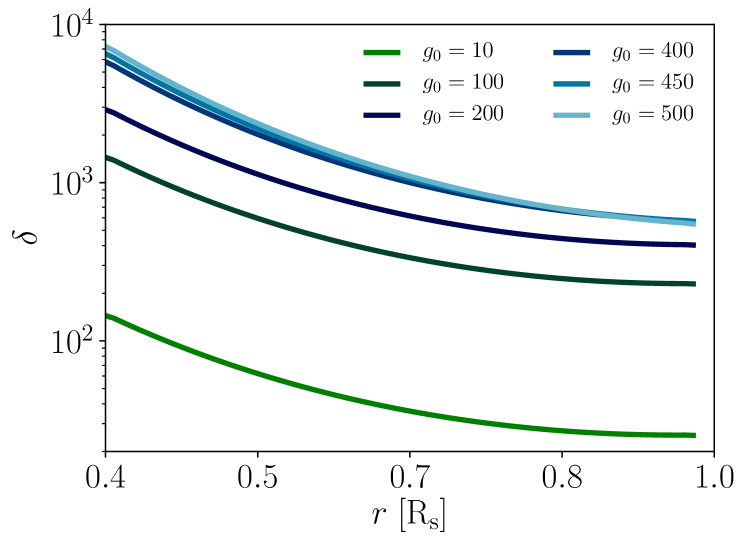
Figure 2: Radial profile of $\delta$ for simulations TiA04, TiA07, TiA09, TiA12, TiA13 and TiA14. These simulations start with the same initial magnetic field, $B_{0}=1$ T, but have different gravity at the bottom of the domain, $g_{0}$.

Model	$g_{0}$	$B_{0}$	$\overline{\omega}_{BV}\cdot 10^{-8}$	$\overline{\omega_{A}}\cdot 10^{-7}$	$\rho_{b}/\rho_{t}$	$\overline{\delta}$	$B_{p}/B_{t}$	$\Gamma$	$k_{r}^{max}$
TiA00	0.01	1.00	1.3567	2.4225	1.00	0.056	0.39	5.388	1.3
TiA01	1	1.00	136.67	2.4239	1.01	5.638	0.46	4.531	3.3
TiA02	5	1.00	683.34	2.4305	1.02	28.115	0.33	3.949	10.2
TiA03	10	1.00	1366.7	2.4384	1.03	56.049	0.17	3.363	12.6
TiA04	30	1.00	4100.2	2.4716	1.11	165.890	0.25	1.573	16.1
TiA05	50	1.00	6833.8	2.5064	1.18	272.656	0.28	0.887	19.5
TiA05rf	50	1.00	6833.8	2.5064	1.18	272.656	0.32	1.071	15.3
TiA06	70	1.00	9567.5	2.5421	1.27	376.360	0.36	0.757	17.0
TiA07	100	1.00	13668	2.5991	1.40	525.882	0.28	0.454	18.5
TiA08	150	1.00	20503	2.7024	1.66	758.719	0.32	0.345	20.2
TiA09	200	1.00	27339	2.8184	1.97	970.048	0.36	0.223	16.7
TiA10	250	1.00	34176	2.9499	2.33	1158.546	0.33	0.178	18.7
TiA11	300	1.00	41014	3.1010	2.76	1322.613	0.17	0.202	22.3
TiA12	400	1.00	54691	3.4857	3.87	1569.008	0.57	0.168	18.7
TiA13	450	1.00	61531	3.7394	4.58	1645.477	0.39	0.174	16.1
TiA14	500	1.00	68372	4.0576	5.42	1685.022	0.70	0.163	15.4
TiAhr00	0.01	1.00	1.3567	2.4206	1.00	0.056	0.57	6.542	0.98
TiAhr01	1	1.00	135.67	2.4222	1.01	5.601	0.64	4.571	5.49
TiAhr02	20	1.00	2713.4	2.4533	1.07	110.603	0.14	3.258	27.47
TiAhr05	50	1.00	6783.6	2.5047	1.18	270.834	-	1.716	41.00
TiAhr14	500	1.00	67859	4.0616	5.49	1670.744	-	0.242	38.18

Table 1: Parameters and results of simulations with fixed magnetic field and different values of $g_{0}$. The table presents the mean Brunt-Vaisala (buoyancy) $\overline{\omega}_{BV}$, and Alfvén, $\overline{\omega_{A}}$ frequencies, the bottom-to-top density contrast $\rho_{b}/\rho_{t}$, the parameter $\overline{\delta}$, the ratio of domain-averaged poloidal and toroidal fields, $B_{p}/B_{t}$, at the end of the linear phase of the instability, the growth rate $\Gamma$, and the maximum vertical wave number, $k_{r}^{max}$. The lowest rows show results from simulations with higher resolution, double of all the others. We report the value of $B_{p}/B_{t}$ only for the simulations that reached the end of the linear growth.

Model	$g_{0}$	$B_{0}$	$\overline{\omega}_{BV}\cdot 10^{-8}$	$\overline{\omega}_{A}\cdot 10^{-7}$	$\rho_{b}/\rho_{t}$	$\overline{\delta}$	$B_{p}/B_{t}$	$\Gamma$	$k_{r}^{max}$
TiB50a	50	0.01	6833.8	2.5064	1.18	27265.642	-	0.174	-
TiB50b	50	0.05	6833.8	12.532	1.18	5453.122	-	0.199	17.3
TiB50c	50	0.10	6833.8	25.064	1.18	2726.574	0.10	0.268	17.4
TiB50d	50	0.50	6833.8	125.32	1.18	545.313	0.25	0.630	18.4
TiB50e	50	0.65	6833.8	162.91	1.18	419.471	0.28	0.771	16.5
TiA05	50	1.00	6833.8	250.62	1.18	272.679	0.36	0.887	19.3
TiB100a	100	0.01	13668	0.0260	1.40	52588.239	-	0.011 ∗	-
TiB100b	100	0.05	13668	0.1299	1.40	10517.648	-	0.044	6.8
TiB100c	100	0.10	13668	0.2599	1.40	5258.824	-	0.134	7.4
TiB100d	100	0.50	13668	1.2996	1.40	1051.765	0.25	0.332	17.7
TiB100e	100	0.65	13668	1.6894	1.40	809.050	0.30	0.406	18.9
TiA07	100	1.00	13668	2.5991	1.40	525.882	0.28	0.454	18.5
TiB150a	150	0.10	20503	0.0270	1.66	75871.9	-	0.010∗	-
TiB150b	150	0.05	20503	0.1351	1.66	15174.38	-	0.032∗	-
TiB150c	150	0.10	20503	0.2702	1.66	7587.189	-	0.039	6.8
TiB150d	150	0.50	20503	1.3512	1.66	1517.44	0.10	0.226	16.4
TiB150e	150	0.65	20503	1.7565	1.66	1167.28	0.26	0.285	17.2
TiA08	150	1.00	20503	2.7024	1.66	758.719	0.32	0.345	20.2

Table 2: Results of simulations with three values of gravity ($g_{0}=50$, $100$, $150$ m s^-2) and changing magnetic field amplitude, $B_{0}$; for each value of $g_{0}$ the magnetic field varies in the range $1$ to $10^{-2}$ T. The parameters are the same as in Table 1. The growth rates marked with ^∗ are compatible with zero, as the relative simulations have never reached the linear growth phase after about 15 $t_{\rm A}$ and they show a noisy behaviour. We decided to include these values anyways for completeness. We report the value of $B_{p}/B_{t}$ only for the simulations that reached the end of the linear growth.

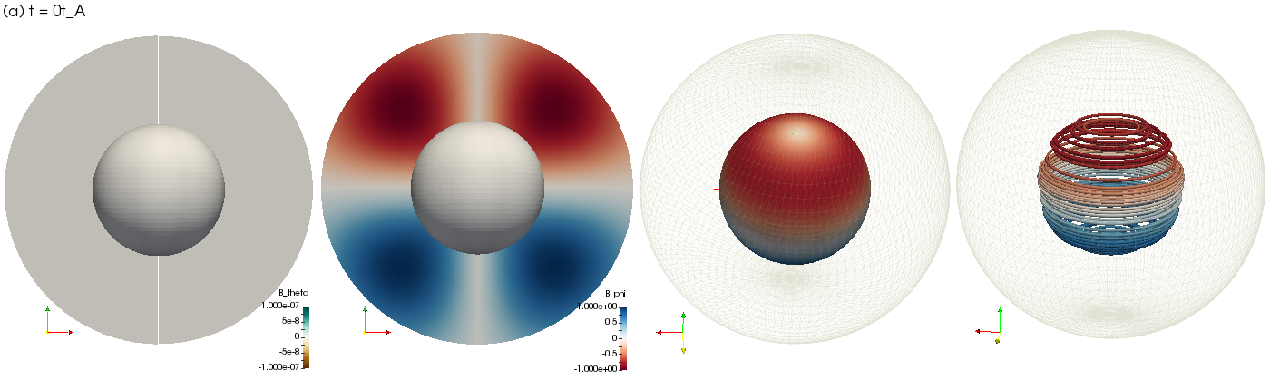
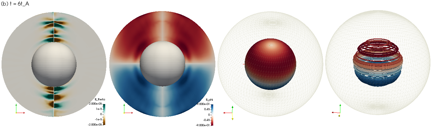
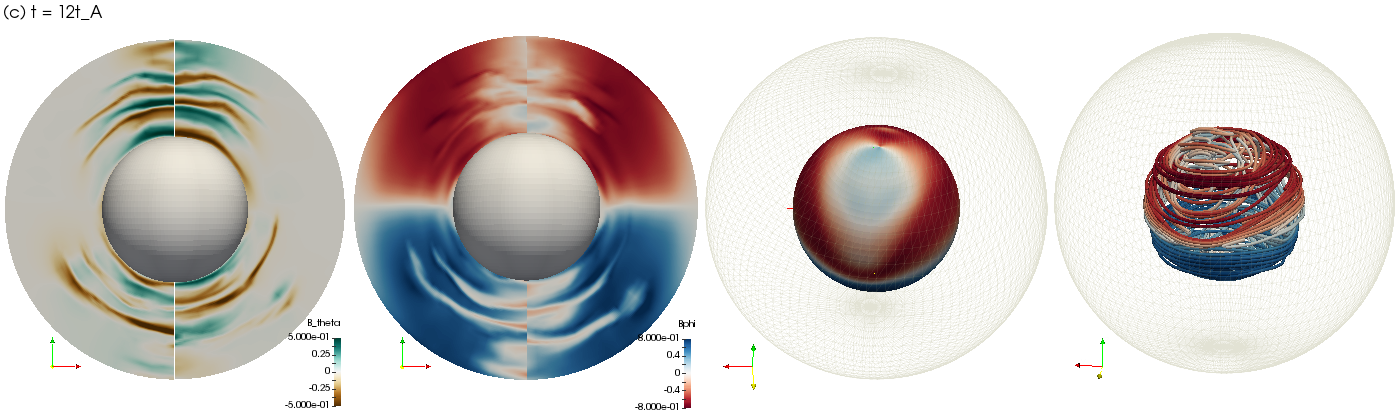
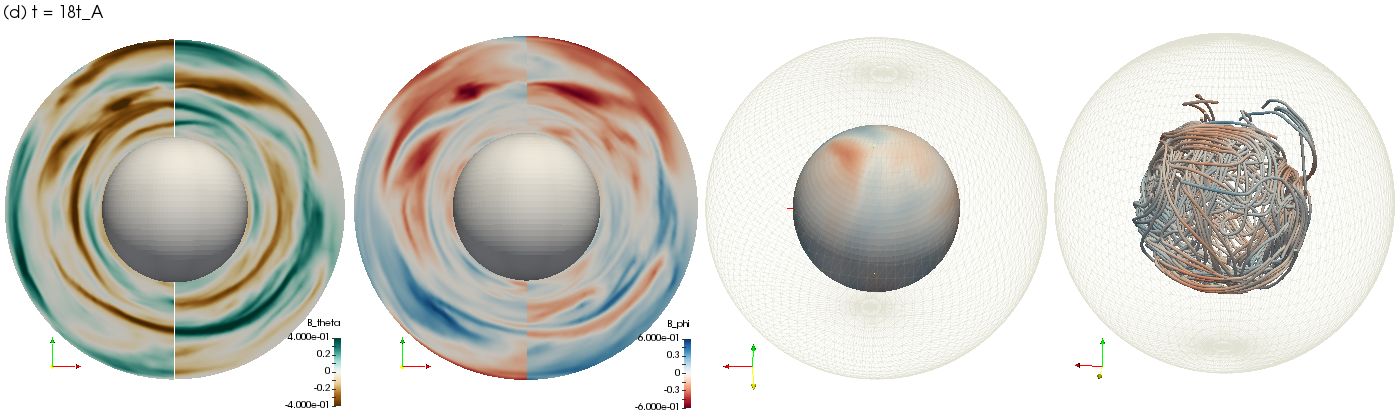
Figure 3: Magnetic field evolution for the simulation TiA01. The first and second columns show contourplots of the latitudinal, $B_{\theta}$, and longitudinal, $B_{\varphi}$, components of the magnetic field in the longitudinal, $r-\theta$, plane for $\varphi=0$ and $\pi$. The third column shows $B_{\varphi}$ on the $\varphi-\theta$ surface at $r=0.45R_{\rm s}$. The fourth shows the magnetic field lines at $r=0.45R_{\rm s}$: the red (blue) color represents a counterclockwise (clockwise) longitudinal field. Different rows correspond to different evolution times in Alfvén travel times: $t=0t_{\rm A},~{}6t_{\rm A},~{}12t_{\rm A},~{}18t_{\rm A}$.

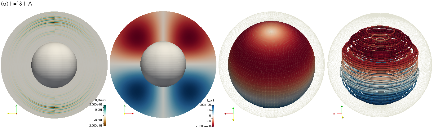
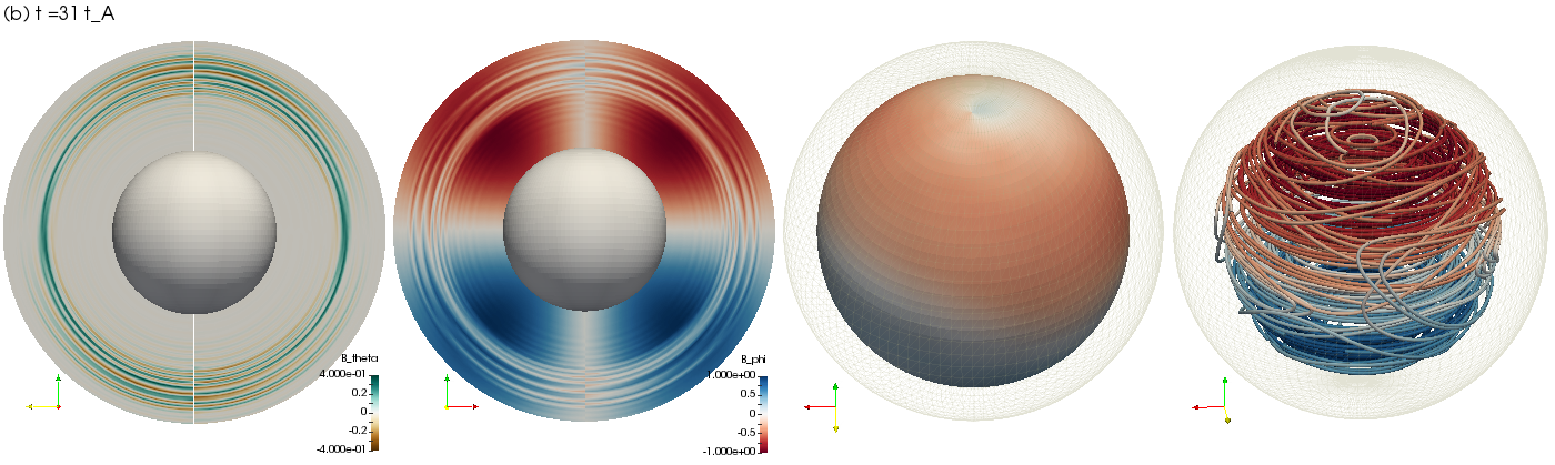
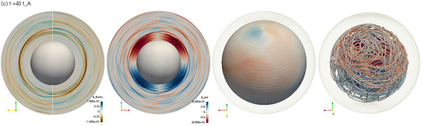
Figure 4: Same as Fig. 3, but for simulation TiA05 at $t=18t_{\rm A},~{}31t_{\rm A},~{}43t_{\rm A}$. In this case the field configurations in third and fourth columns are shown at $r=0.85R_{\rm s}$.

3 Global numerical simulations

To overcome the limitations of the earlier analytical considerations we perform global numerical simulations with the EULAG-MHD code. We study the non-rotating case by solving the anelastic MHD equations in the following form:

$${\bm{\nabla}}\cdot(\rho_{\rm ad}\bm{u})=0,$$ (7)

$$\frac{D\bm{u}}{Dt}=-{\bm{\nabla}}\left(\frac{p^{\prime}}{\rho_{\rm ad}}\right)+{\bm{g}}\frac{\Theta^{\prime}}{\Theta_{\rm ad}}+\frac{1}{\mu_{0}\rho_{\rm ad}}({\bm{B}}\cdot\nabla){\bm{B}}\;,$$ (8)

$$\frac{D\Theta^{\prime}}{Dt}=-{\bm{u}}\cdot{\bm{\nabla}}\Theta_{\rm amb}-\frac{\Theta^{\prime}}{\tau}\;,$$ (9)

$$\frac{D{\bm{B}}}{Dt}=({\bm{B}}\cdot\nabla){\bm{u}}-{\bm{B}}(\nabla\cdot{\bm{u}})\;,$$ (10)

where $D/Dt=\partial/\partial t+\bm{u}\cdot{\bm{\nabla}}$ is the total time derivative, ${\bm{u}}$ is the velocity field, $p^{\prime}$ is a pressure perturbation variable that accounts for both the gas and magnetic pressure, and ${\bm{B}}$ is the magnetic field. The energy equation (9) is written in terms of perturbations of the potential temperature, $\Theta^{\prime}$, with respect to the ambient state, $\Theta_{\rm amb}$. The latter is chosen to be roughly isothermal (see Guerrero et al., 2013; Cossette et al., 2017, for comprehensive discussions about this formulation of the energy equation). The $\rho_{\rm ad}$ and $\Theta_{\rm ad}$ are the density and potential temperature of the reference isentropic state (i.e., $\Theta_{\rm ad}={\rm const}$) in hydrostatic equilibrium: the potential temperature, $\Theta^{\prime}$, is related to the specific entropy by $ds=c_{p}d\ln\Theta^{\prime}$; $g=\frac{g_{0}}{(r/r_{b})^{2}}\bm{\hat{e}}_{r}$ is the gravity acceleration, with $g_{0}$ its value at the bottom of the domain where $r=r_{b}$; and $\mu_{0}$ is the magnetic permeability of the vacuum; the last term in equation 9 is a Newtonian cooling that relaxes $\Theta^{\prime}$ in a time scale $\tau=1.296\times 10^{7}$ s. For the simulations presented here this time scale is shorter than the average Alfvén travel time $t_{\rm A}=2\pi/\omega_{A}$ (see Eqs. 6 and 15).

The Newtonian cooling acts in the simulations as scale independent thermal diffusion that substitutes the thermal and radiative diffusion expected to exist in stellar interiors. The value that we use is a compromise between having a fast cooling or a slow thermal diffusion given only by the numerical resolution, therefore allowing large values of $\Theta^{\prime}$. We verified the effects of this term by running auxiliary simulations (not shown) with different values of $\tau$. In cases where the Newtonian cooling is 100 times shorter, i.e., $\tau=1.296\times 10^{5}$ s, the instability is partially suppressed. In simulations where the Newtonian cooling term is removed (i.e., $\tau\rightarrow\infty$) we observe an overall behaviour similar to the simulations with our fiducial value of $\tau=1.296\times 10^{7}$ s. Nevertheless, the average values of the growth rate of the instability are somewhat smaller. This is consistent with the findings of the linear theory by Bonanno & Urpin (2012), and demonstrate that the thermal diffusivity enhances instability.

We consider a spherical shell with $0\leq\varphi\leq 2\pi$, $0\leq\theta\leq\pi$ and a radial extent from $r_{b}=0.4R_{\odot}$ to $r_{t}=0.96R_{\odot}$. The boundary conditions are defined as follows: for the velocity field we use impermeable, stress-free conditions at the top and bottom surfaces of the shell; for the magnetic field we consider a perfect conductor at both boundaries. Finally, for the thermal boundary condition we consider zero radial flux of potential temperature. The discrete mesh in most of the simulations has $126\times 42\times 72$ grid points in the $\varphi$, $\theta$ and $r$ directions, respectively. The constant time-step of the simulations is $\Delta t=1800$ s. For the high resolution simulations we double the number of grid points in each direction and decrease the time-step to $\Delta t=450$ s. The reference and ambient states are computed by solving the hydrostatic equilibrium equations for a polytropic atmosphere,

$$\frac{\partial T_{\rm i}}{\partial r} = -\frac{g}{R_{g}(m_{\rm i}+1)}\;,$$ (11)

$$\frac{\partial\rho_{\rm i}}{\partial r} = =-\frac{\rho_{\rm i}}{T_{\rm i}}\left(\frac{g}{R_{g}}-\frac{\partial T_{\rm i}}{\partial r}\right)\;,$$ (12)

where the index ${\rm i}$ stands either for ${\rm``ad"}$ or ${\rm``amb"}$, $R_{g}=13732$ is the gas constant. Density and temperature are related to the gas pressure through the equation of state for a perfect gas, $p_{\rm i}=R_{g}\rho_{\rm i}T_{\rm i}$. The bottom boundary values used to integrate (11) and (12) are $T_{b}=3.5\times 10^{6}$ K and $\rho_{b}=37~{}{\rm kg}~{}{\rm m}^{-3}$, respectively. Different values of $g_{0}$ allow to obtain different degrees of stratification. Finally, adiabatic and roughly isothermal atmospheres are obtained with the polytropic indexes $m_{\rm ad}=1.5$ and $m_{\rm amb}=10^{3}$, respectively.

The simulations start with a purely toroidal magnetic field,

$$B_{r0}=0~{},\;B_{\theta 0}=0~{},\;B_{\varphi 0}=B_{0}f(r)\sin 2\theta\;,$$ (13)

with

$$f(r)=\exp\left(-(r-r_{0})^{2}/d^{2}\right),$$ (14)

where $r_{0}=0.68R_{\odot}$, $d=0.5R_{\odot}$, and $B_{0}$ is the maximum amplitude of the initial magnetic field which is a free parameter in the simulations (see Table 1 and 1).

To directly compare the 3D simulations with the linear analysis we consider the non-dimensional quantity $\delta^{2}$, defined in Eq. (6). However, in the global models we have a gravity profile depending on radius, and an initial magnetic field depending on $r$ and $\theta$; see Fig. 2. Thus, we consider $\overline{\delta}^{2}=\overline{\omega}_{BV}^{2}/\overline{\omega}_{A}^{2}$, with

$$\overline{\omega}_{BV}^{2}=\langle\frac{g}{\Theta_{\rm amb}}\frac{\partial\Theta_{\rm amb}}{\partial r}\rangle_{r},\;\;\overline{\omega}_{A}^{2}=\langle\frac{B_{\varphi 0}^{2}}{\mu_{0}\rho_{\rm amb}d^{2}}\rangle_{r,\theta}.$$ (15)

Here, the angular brackets represent averages in the radial direction for the Brunt-Vaisäla and in radius and latitude (over one hemisphere) for the Alfvén frequency. The values of $\overline{\omega}_{BV}$, $\overline{\omega}_{A}$ and $\overline{\delta}$ are presented in Table 1.

By construction our initial state is Tayler unstable. Therefore, it is expected that the instability develops after a few characteristic Alfvén travel times $t_{\rm A}$. As we will see, this occurs quickly for the models with strongest initial magnetic fields. On the other hand, the simulations with weaker fields ($B_{0}\leq 0.5$ T) reach magnetohydrostatic equilibrium after about one $t_{A}$. Therefore, to excite the instability we impose a white noise perturbation with amplitude of $10^{-3}$ m s^-1 and continue the simulations for, at least, $20t_{\rm A}$.

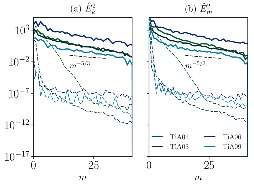
Figure 5: Kinetic (a) and magnetic (b) energy density spectra as a function of the longitudinal wave number $m$, measured during the linear (dashed lines) and the dissipative (solid) phases, of some characteristic simulations. The black dashed lines correspond the $m^{-5/3}$ scaling law.

4 Results

In the first set of simulations we start with a strong initial magnetic field, $B_{0}=1$ T, and vary the gravity at the bottom of the domain, $g_{0}$, from $0.01$, that means that the density is roughly constant in radius, to $500$ m s^-2, corresponding to a density contrast $\sim 5.5$. In the weak gravity cases, $g_{0}=0.01$ and $1$ m s^-2, we observe the instability to develop fast, on a time scale of the order of one $t_{\rm A}$. Figure 3 depicts the temporal evolution of the latitudinal, $B_{\theta}$, and longitudinal, $B_{\varphi}$, magnetic field components for the simulation TiA01, with $g_{0}=1$ m s^-2. The first and second columns show, respectively, contours of $B_{\theta}$ and $B_{\varphi}$ in the meridional plane, $r-\theta$, for $\varphi=0$ and $\pi$. The third column shows $B_{\varphi}$ in the horizontal, $\varphi-\theta$, plane at $r=0.45R_{\rm s}$. Red (negative) and blue (positive) contours correspond to counterclockwise and clockwise toroidal fields, respectively. The right column shows the magnetic field lines at $r=0.45R_{\rm s}$ colored according to the amplitude of $B_{\varphi}$. The upper row (a) corresponds to the initial configuration; Eq. (13). The second row (b) corresponds to the linear phase of the instability at $t=6t_{\rm A}$. The development of $B_{\theta}$ with a $m=1$ symmetry starting from the axial cylinder is evident. The decay of $B_{\varphi}$ occurs in this phase predominantly in the $m=0$ mode which still has larger energy. Thus, the magnetic field lines do not show any significant change with respect to the initial state. The third row (c) corresponds to the end of the linear phase, $t=12t_{\rm A}$. At this stage the non-axisymmetric mode, $m=1$, has a larger energy which is evident in $B_{\theta}$ as well as in $B_{\varphi}$. The instability seems to be occurring in different radial layers of magnetic field and propagating from the vertical axis of the sphere, $\varphi=\theta=0$. towards equatorial latitudes. The rightmost columns show the field morphology in the innermost layers. The bottom row (d) corresponds to the beginning of the dissipative phase. It is clear in the panels of this row that although high order modes develop, the mode $m=1$ still prevails at some radial levels.

Figure 4 depicts the development of the Tayler instability for simulation TiA05, with $g_{0}=50$ m s^-1. In this figure, however, the third and fourth columns show the magnetic field at $r=0.85R_{\rm s}$. Since the initial configuration is the same for all cases, we present only the magnetic field after (a) $\sim 18t_{\rm A}$, corresponding to the linear phase, (b) $\sim 31t_{\rm A}$, corresponding to the saturated phase and (c) $\sim 43t_{\rm A}$ when the field is in the diffusive decaying stage. Similar to the case TiA01, the instability starts close to the axis and propagates towards the equator. Nevertheless, it occurs in a larger number of radial layers with different growth rates. The panels in the bottom row indicate that the instability is fully developed at the upper radial levels but at the bottom of the domain the field conserves some coherence. The magnetic field lines, fourth column, show a fully mixed magnetic field at $r=0.85R_{\rm s}$ but suggest a better organized field in deeper layers.

In Fig. 5 we present the energy density spectra of the velocity and magnetic fields at the linear (dashed lines) and the dissipative (solid lines) phases, for some characteristic simulations (the decomposition in spherical harmonics was performed with the optimized library SHTns Schaeffer, 2013) . We observe that in the simulation TiA01, characterized by small $\overline{\omega_{\rm BV}}$, during the linear phase most of energy is stored in about 20 longitudinal modes. As $\overline{\omega_{\rm BV}}$ increases, the number of longitudinal modes decreases. On the other hand, when the system reaches the dissipative phase, we observe the occurrence of fully developed 3D turbulence independently of the stratification: this is illustrated by the behavior of the kinetic and magnetic energy power spectra, which exhibit a $m^{-5/3}$ power law decay.

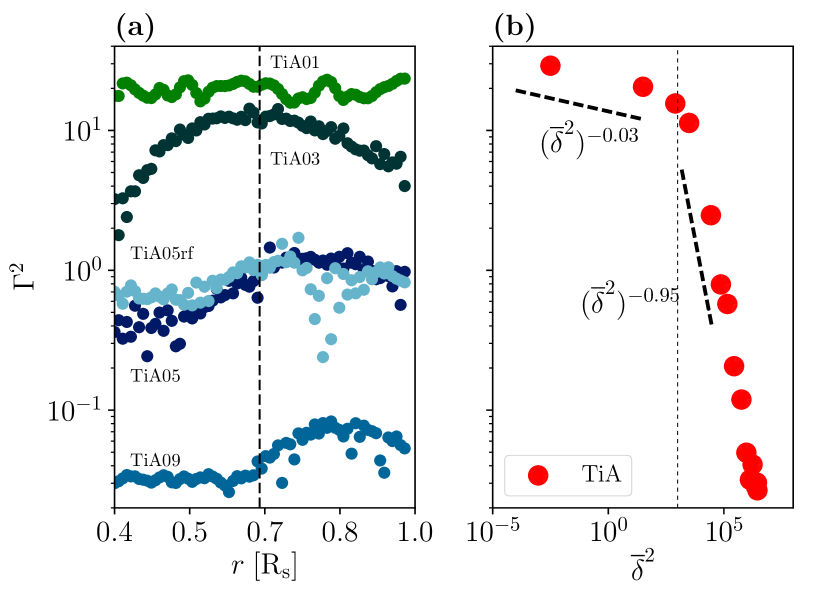
Figure 6: (a) Growth rate squared, $\Gamma^{2}$, of the Tayler instability as a function of radius for some characteristic simulations with different $g_{0}$. The vertical dashed line corresponds to the radius where the initial magnetic field is maximum. (b) $\Gamma^{2}$ as a function of $\delta^{2}$ for the set of simulations TiA. The growth rate corresponds to $r=0.68R_{\rm s}$. Here the vertical dashed line shows approximatively the separation between the two regimes $\Gamma^{2}\propto\delta^{-0.03}$ and $\Gamma^{2}\propto\delta^{-0.95}$.

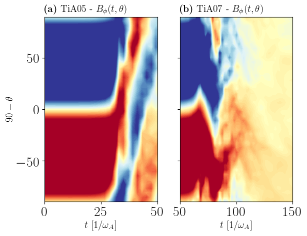
Figure 7: Time-latitude evolution of the toroidal magnetic field at $\varphi=90^{\circ}$ and $r=0.72R_{s}$ for the simulations (a) TiA05 and (b) TiA07.

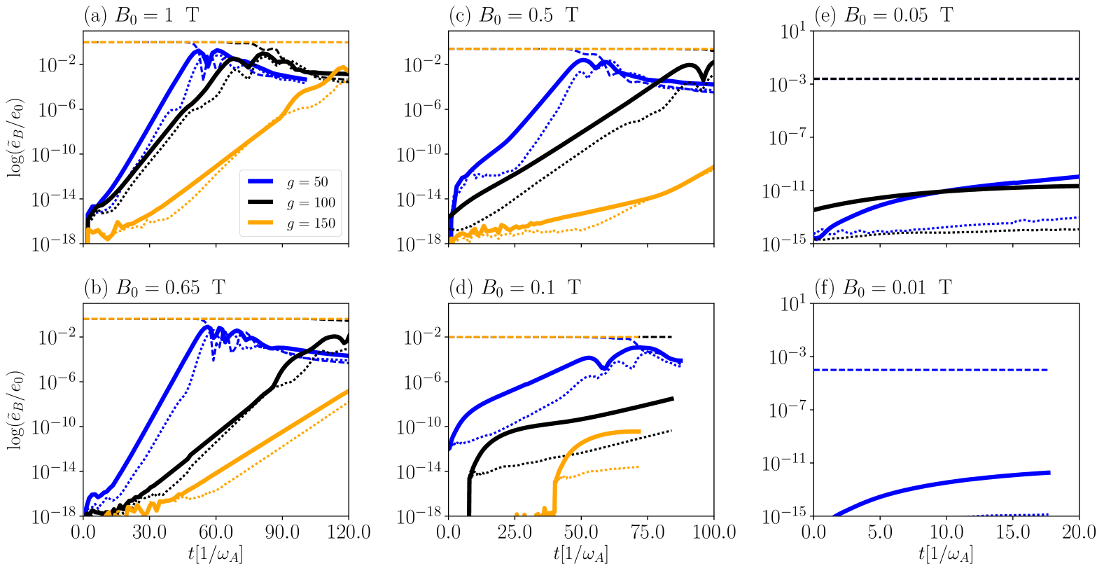
Figure 8: Time evolution of the simulations in Table 2. Different colors correspond to different values of $g_{0}$ as shown in the legend. The dashed, solid and dotted lines correspond to the modes $m=0,1$ and $2$, respectively.

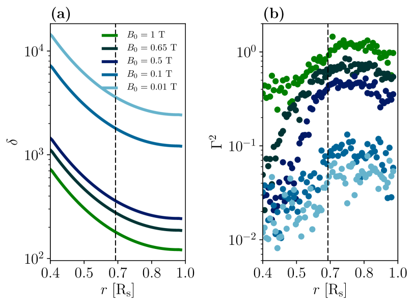
Figure 9: (a) Radial profile of $\delta$ for simulations with fixed $g_{0}=50$ m s^-2, and magnetic field with maximum amplitude, $B_{0}$ between $1$ and $0.01$ T. (b) Growth rate squared, $\Gamma^{2}$, as a function of radius for these simulations. The vertical dashed lines corresponds to the radius where the initial magnetic field is maximum.

Since the development of the Tayler instability occurs at different time scales for different depths, we compute the growth rate, $\Gamma$, of the instability at each radial point. $\Gamma$ is estimated from the time evolution of the mode $m=1$ of the magnetic field energy density. In Fig. 6(a) we present the growth rate of the Tayler instability, in Alfvén travel times $t_{\rm A}$, as a function of radius for some characteristics simulations with different values of $g_{0}$. We notice that the growth rate of the instability is roughly independent of radius for small $g_{0}$, i.e., small $\overline{\delta}$. Yet, when $\overline{\omega_{\rm BV}}$ increases, the growth rate is smaller at the bottom of the domain where $\delta$ has larger values. It reaches a maximum at a radius that seems to increase with $g_{0}$, and then decreases again near the upper boundary. For the cases with larger $g_{0}$ (simulations TiA09-TiA14), the growth rate is constant in the lower half of the domain; e.g., see the points corresponding to simulation TiA09 in Fig. 6(a)). To study the role of the magnetic boundary condition on the growth rate we performed one simulation, TiA05rf, with pseudo-vacuum boundary condition at the upper boundary. Even though the radial profile of $\Gamma$ is slightly different, on average the growth rate agrees with that of the simulation with perfect conductor boundary condition (see light blue points in Fig. 6(a) as well as Fig. 10).

Figure 6(b) shows $\Gamma^{2}$ at $r=0.68R_{\rm s}$ (where the initial toroidal magnetic field has a maximum) as a function of $\overline{\delta}$ for all simulations with $B_{0}=1$ T. The growth rate follows two different behaviors. For $\delta\lesssim 50$ (see the vertical dotted line) the growth rate is large and decays slowly following the power law $(\delta^{2})^{-0.03}$. For $\delta\gtrsim 50$ the decay of the growth rate is fast and follows the power law $\Gamma^{2}\propto(\delta^{2})^{-0.95}$. In this region $\Gamma^{2}$ changes by a factor of $10^{2}$. For larger values of $g_{0}$; ($\overline{\delta}^{2}\gtrsim 10^{6}$), the growth rate remains approximately constant. This is expected since increasing $g_{0}$ above 200 m s² results in adjacent BV frequency profiles as can be seen in Fig. 2. The trend $\Gamma^{2}\propto(\delta^{2})^{-0.95}$ depicted in Figs. 6(b) and 10 is consistent with the findings of Bonanno & Urpin (2012), who used eq.(2) and obtained a stabilizing effect of gravity with a power law $\Gamma^{2}\propto(\delta^{2})^{-1}$. Also, $\Gamma$ can attain values smaller than 1, in agreement with findings of Goldstein et al. (2019)

In Table 1 we also report a measurement of the ratio of mean poloidal and toroidal fields, calculated over the entire domain at the end of the linear growth of the instability. Whilst we could not identify an explicit dependence of this ratio on the initial values of the parameters $g_{0}$ and $B_{0}$, it is clear that a poloidal component of the field develops, and it keeps growing during the nonlinear phase.

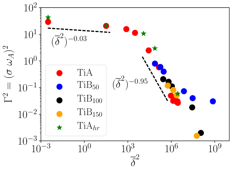
Figure 10: Dimensionless growth rate squared for the mode $m=1$, as a function of $\overline{\delta}^{2}$ for the models in Tables 1 and 2.

4.1 The role of initial magnetic field strength

To further increase the value of $\overline{\delta}$ we run three sets of simulations where $g_{0}$ is either $50$, or $100$ or $150$ m s^-2. For each of them, we explore the role of the initial magnetic field strength, by varying its maximum amplitude, $B_{0}$, from $1$ down to $0.01$ T.

The results of these simulations are presented in Table 2, and the time evolution for the these sets is depicted in Fig. 8(a)-(f). Each panel shows the results for different field amplitudes, with the blue, black and yellow lines corresponding to $g_{0}=50$, $100$ and $150$ m s^-2, respectively. The dashed, solid and dotted lines correspond to the longitudinal modes, $m=0$, $1$ and $2$, respectively. The results confirm that the behavior described above for $B_{0}=1$ T holds also for smaller values of the initial field, i.e., the stronger the gravity force, the smaller the instability growth rate. As mentioned above, for large values of $B_{0}$ the instability starts developing after 1-3 $t_{\rm A}$, without the need of perturbing the system. For $B_{0}\leq 0.1$ T the initial magnetic field remains stationary while the velocity field and the potential temperature adapt to magneto-hydrostatic equilibrium. We run these initial states for $\sim 10\;t_{A}$. The instability develops after perturbing the system with white noise in the potential temperature perturbations. For some of the simulations, instead, the instability doesn’t develop even after perturbing the system, illustrating how the system is stabilized by the combination of strong gravity and weak fields. Figure 8(a)-(d) show that in most of the simulations the end of the linear growing phase is characterized by oscillations. These patterns resemble the results by Weber et al. (2015), who found helicity oscillations in simulations of the Tayler instability in cylindrical coordinates. In our case we notice that they correspond to waves of magnetic field that travel from one pole to the other. Figure 7(a) and (b) show the time evolution of the toroidal magnetic field of simulations TiA05 and TiA07 to illustrate this pattern. The toroidal field is sampled at a longitude of $90^{\circ}$ and a radius of $r=0.76R_{s}$. The migration direction might change for different choices of longitude and is more evident at a radius closer to the maximum of the initial toroidal field. The oscillations seem to have longest period for simulations with small $\overline{\delta}$ and are not clearly defined in simulations with $\overline{\delta}\gtrsim 10^{3}$. This pattern rapidly disappears once the field enters in the dissipative phase.

In Fig. 9 we compare the radial profiles of (a) $\delta$, and (b) $\Gamma^{2}$ as function of radius in simulations with $g_{0}=50$ m s^-2 and different values of $B_{0}$. The figure indicates that for all the cases the instability growth rate is smaller at the bottom (where $\delta$ is larger) and larger and the top (small $\delta$). Also, the maximum of the growth rate appears roughly at the same radius, $r\sim 0.75R_{\rm s}$, in all simulations. Nevertheless, while for the smaller values of $\delta$ (i.e., for $B_{0}>0.5$ T) the profiles of $\Gamma^{2}$ have a clear radial trend, for higher $\delta$ (i.e., $B_{0}\leq 0.1$ T) the growth rate shows a significant dispersion. For this reason, the growth rate presented in Table 2 corresponds to the radial average of $\Gamma$ between $0.66r/R_{\rm s}$ and $0.7r/R_{\rm s}$.

The combination of strong gravity and weak magnetic field allows to reach $\overline{\delta^{2}}\sim 10^{9}$ (Table 2), These results are presented in Fig. 10 where the red points are the same presented in Fig. 10, and the blue, black and yellow points correspond to $g_{0}=50$, $100$ and $150$ m s^-2, respectively. The results suggest that for each set of simulations in Table 2 there is a power law decay. Nevertheless, for the large values of $g_{0}$ considered (i.e., $100$ and $150$ m s^-2), the exponent seems to be similar. The figure clearly evidences that gravity inhibits the instability of the magnetic field by changing $\Gamma^{2}$ by several orders of magnitude.

The combination of strong gravity ($g_{0}=100$, $150$ m s^-2) and weak fields ($B_{0}\leq 0.05$ T) results in growth rates almost negligible. This is a consequence of the stabilizing effect of gravity. We notice, however, that simulations with small $B_{0}$, are characterized by longer Alfvén travel times. Thus, these simulations require a much longer computational time which at the moment is prohibitive. So these simulations have not reached saturation, and the possibility that the systems will become unstable on scales of the order of $t\sim 100t_{A}$ cannot be apriori excluded. Nonetheless, there is a clear trend showing that weaker magnetic fields are stable on longer timescales.

4.2 Effects of resolution

We also explore the role of resolution in our simulations by doubling number of cells in all directions, i.e., considering $252\times 84\times 144$ grid points in $\varphi$, $\theta$ and $r$, respectively. We observe that the values of $\Gamma$ for each $\overline{\delta}$ are slightly larger than their low-resolution counterparts (see simulations TiAhr00-TiAhr14 in Table 1). Nonetheless, it is interesting to notice that in the simulations with higher resolution the trend of $\Gamma$ as a function $\overline{\delta}$ seems to be the same as for the lower resolution case. The two regimes described above are discernible in Fig. 10 (see the green stars). This confirms that our numerical approach is able to capture the stabilizing effect of gravity.

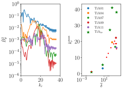
Figure 11: Left: Fourier energy spectra in the radial direction as a function of the vertical wave number, $k_{r}$, for some characteristic simulations. Right: Maximum vertical wave number as function of $\overline{\delta}$. The color points correspond to the simulations indicated in the legend. The red points show the results for the all other low resolution simulations in Table 1, whilst the green stars correspond to the high-resolution simulations.

4.3 Radial modes

While studying the temporal evolution of the simulations we noticed that increasing the value of $\overline{\delta}$ by increasing $g_{0}$ leads to a larger number of radial modes (see Figs. 3 and 4). We quantify this number by computing the spectra of kinetic and magnetic energy density through a Fourier analysis. The results presented in Fig. 11 and in Tables 1 and 2 shows that the radial wave number, $k_{r}$, increases with delta following a power law. However, for the $g_{0}\gtrsim 100$ the number of radial modes oscillates around $\sim 18$. This is expected since the values and profiles of $\delta$ do not significantly change for these gravity values, similarly, the growth rates are all around the same values.

For simulations with constant $g_{0}=50,100$ or $150$, and varying initial field strength, $B_{0}$, the number of radial modes is similar, fluctuating about 18 (for clarity these simulations have not been included in Fig. 11). On the other hand, the simulations with high-resolution develop a number of radial modes that doubles that of the low-resolution cases at the same $\delta$ (see the green stars in Fig. 11). We also notice that the number of modes changes with time, but for each simulation we can identify a portion of the linear phase of the instability where the number of modes stays almost constant, and it attains the same value both for the magnetic and the velocity fields. This is the number we report in in Tables 1 and 2. These findings indicate that the Tayler instability has a radial dependence for small values of $\overline{\omega_{\rm BV}}$ only. When the Brunt-Väisäla frequency exceeds a value about $10^{-4}$ Hz, the instability becomes independent of the stratification. In other words, it becomes bidimensional in nature. We interpret this as a numerical effect, where a few grid points in the radial directions are required for the initial magnetic field to decay into a mixed, toroidal-poloidal configuration, through reconnection processes.

5 Conclusions

We present global anelastic simulations of the evolution of toroidal magnetic fields in a stable stratified, roughly isothermal, environment. The initial field configuration is consistent with two bands of toroidal field antisymmetric across the equator. We study the development of the Tayler instability and assess the role played by the Brunt-Väisäla and the Alfvén frequencies on its characteristics. We do this by changing the gravity, $g_{0}$, and the initial magnetic field strenght, $B_{0}$.

As expected, the fastest growing mode is $m=1$. Nevertheless, other longitudinal modes also develop; for the lower values of $g_{0}$ other large scale modes develop until $m\sim 20$. As $g_{0}$ increases only large scale modes grow during the linear phase, i.e., $m\lesssim 3$. In the radial direction the behavior is similar, the stronger the gravity the larger the number of modes, and the instability appears to develop roughly horizontally. The maximum number of radial modes, $k^{max}_{r}$, reaches some saturation for large $g_{0}$, and this number doubles when we double the resolution of the simulations. We interpret this as a numerical constrain from the inviscid numerical technique of the EULAG-MHD code for the magnetic field to evolve. This suggests that the number of radial modes might depend on the value of the magnetic diffusivity, $\eta$, i.e., in ideal MHD the evolution of the field in stable stratified layers might be bi-dimensional.

When reaching the saturated phases of the instability the time-series of the simulations exhibit oscillations. We identified these as waves of magnetic field that travel from one hemisphere to the other. After one or two periods these oscillations disappear as the magnetic field reaches the dissipative phase. We can speculate that these oscillations will continue and sustained dynamo action might appear if differential rotation is present in these layers. It should replenish the toroidal magnetic field, later on achieving cyclic behavior. In the dissipative phase of the simulations presented here, fully developed MHD turbulence is observed during this stage. Most of the energy density is in the large-scale modes, $m=0$ and $1$, and an energy cascade that roughly goes as $m^{-5/3}$ is observed.

The growth rate of the Tayler instability as a function of $\overline{\delta}$, averaged ratio between the BV and the Alfvén frequencies, shows two regimes. For $\overline{\delta}\lesssim 50$ ($g_{0}\lesssim 10$), $\Gamma^{2}\propto\delta^{-0.03}$. For larger values of $\delta$, $\Gamma^{2}\propto\delta^{-0.95}$ (Fig. 6). When the value of $\delta$ is increased by decreasing the initial field, $B_{0}$, this trend seems to be different for low values of $g_{0}$, but converges to $\delta^{-0.95}$ for $g_{0}=100$ and $150$ m s^-2. In the cases of weaker initial magnetic fields we observe a clear suppression of the instability. The simulations do not go unstable for $B_{0}=0.01$ T on timescales of about 15 Alfvén travel times. Nonetheless we cannot exclude the instability will occur later on, after more than hundred $t_{A}$. The transition between the two observed regimes might be connected with the existence of a threshold for the magnetic field strength observed in Ap/Bp stars. For a given $\omega_{\rm BV}$, only sufficiently strong magnetic fields become unstable and may escape to the outer layers of the star, whilst weaker magnetic fields are still unstable but with a much smaller growth rate, comparable with the inverse lifetime of the star. For future work it will be needed to examine the case where the initial field has a poloidal component, since in this case the Tayler instability may behave differently (Duez et al., 2010).

It will also be necessary to explore the effects of rotation and shear: we expect that, on one hand, rotation can stabilize the initial toroidal field, whilst, on the other, shear may act as a source of the magnetic field. In this sense, the Tayler instability is known to be a symmetry breaking process, able to give rise to a saturated helical state starting from an infinitesimal helical perturbation (Bonanno et al., 2012). A possible dynamo effect might occur from the interplay between shear and Tayler instability. This processes needs to be investigated in the framework of global simulations used in this work.

Finally, it is worth repeating the experiments with realistic stratification profiles of A/B stars. For fiducial profiles of the gravity acceleration, the field might either remain confined to the interior or emerge towards the upper layers. In the latter case the use of open magnetic boundaries, i.e., vacuum or pseudo-vacuum, which could drive stellar winds, is necessary. Mass loss through a stellar wind (Alecian & Stift, 2019) as well as atomic diffusion (Deal et al., 2016) are believed to play a significant role in explaining why magnetic A and B stars are chemically peculiar. Furthermore, there is a need to explore the dynamics of the magnetic field in the presence of thermohaline convection due to inhomogeneities in the plasma composition (e.g. Traxler et al., 2011). Having in hand more realistic models, we will be able to evaluate the surface poloidal-to-toroidal field ratio as well as other diagnostics which could be directly compared to spectropolarimetric observations (e.g. Oksala et al., 2018).

References

- Alecian & Stift (2019) Alecian G., Stift M. J., 2019, MNRAS, 482, 4519
- Arlt et al. (2007) Arlt R., Sule A., Rüdiger G., 2007, A&A, 461, 295
- Aurière et al. (2007) Aurière M., et al., 2007, A&A, 475, 1053
- Beck et al. (2012) Beck P. G., et al., 2012, Nature, 481, 55
- Berdyugina (2009) Berdyugina S., 2009, Proceedings of the International Astronomical Union, 259
- Bonanno & Urpin (2012) Bonanno A., Urpin V., 2012, ApJ, 747, 137
- Bonanno & Urpin (2013a) Bonanno A., Urpin V., 2013a, ApJ, 766, 52
- Bonanno & Urpin (2013b) Bonanno A., Urpin V., 2013b, ApJ, 766, 52
- Bonanno et al. (2012) Bonanno A., Brandenburg A., Del Sordo F., Mitra D., 2012, Phys. Rev. E, 86, 016313
- Braithwaite (2008) Braithwaite J., 2008, MNRAS, 386, 1947
- Braithwaite & Nordlund (2006) Braithwaite J., Nordlund Å., 2006, A&A, 450, 1077
- Cossette et al. (2017) Cossette J.-F., Charbonneau P., Smolarkiewicz P. K., Rast M. P., 2017, ApJ, 841, 65
- Deal et al. (2016) Deal M., Richard O., Vauclair S., 2016, A&A, 589, A140
- Donati & Landstreet (2009) Donati J.-F., Landstreet J. D., 2009, ARA&A, 47, 333
- Duez et al. (2010) Duez V., Braithwaite J., Mathis S., 2010, ApJL, 724, L34
- Ferrario (2018) Ferrario L., 2018, Contributions of the Astronomical Observatory Skalnate Pleso, 48, 15
- Ferrario et al. (2009) Ferrario L., Pringle J. E., Tout C. A., Wickramasinghe D. T., 2009, MNRAS, 400, L71
- Fuller et al. (2015) Fuller J., Cantiello M., Stello D., Garcia R. A., Bildsten L., 2015, Science, 350, 423
- Gaurat et al. (2015) Gaurat M., Jouve L., Lignières F., Gastine T., 2015, A&A, 580, A103
- Ghizaru et al. (2010) Ghizaru M., Charbonneau P., Smolarkiewicz P. K., 2010, ApJL, 715, L133
- Goldstein et al. (2019) Goldstein J., Townsend R. H. D., Zweibel E. G., 2019, ApJ, 881, 66
- Goossens et al. (1981) Goossens M., Biront D., Tayler R. J., 1981, Ap&SS, 75, 521
- Guerrero et al. (2013) Guerrero G., Smolarkiewicz P. K., Kosovichev A. G., Mansour N. N., 2013, ApJ, 779, 176
- Guerrero et al. (2019) Guerrero G., Zaire B., Smolarkiewicz P. K., de Gouveia Dal Pino E. M., Kosovichev A. G., Mansour N. N., 2019, ApJ, 880, 6
- Ibáñez-Mejía & Braithwaite (2015) Ibáñez-Mejía J. C., Braithwaite J., 2015, A&A, 578, A5
- Jouve et al. (2015) Jouve L., Gastine T., Lignières F., 2015, A&A, 575, A106
- Kitchatinov (2008) Kitchatinov L. L., 2008, Astronomy Reports, 52, 247
- Kitchatinov & Rüdiger (2008) Kitchatinov L., Rüdiger G., 2008, A&A, 478, 1
- Mathys (2012) Mathys G., 2012, in Shibahashi H., Takata M., Lynas-Gray A. E., eds, Astronomical Society of the Pacific Conference Series Vol. 462, Progress in Solar/Stellar Physics with Helio- and Asteroseismology. p. 295
- Oksala et al. (2018) Oksala M. E., Silvester J., Kochukhov O., Neiner C., Wade G. A., MiMeS Collaboration 2018, MNRAS, 473, 3367
- Paunzen et al. (2005) Paunzen E., Pintado O. I., Maitzen H. M., Claret A., 2005, MNRAS, 362, 1025
- Pitts & Tayler (1985) Pitts E., Tayler R. J., 1985, MNRAS, 216, 139
- Prusa et al. (2008) Prusa J., Smolarkiewicz P., Wyszogrodzki A., 2008, Computers & Fluids, 37, 1193
- Schaeffer (2013) Schaeffer N., 2013, Geochemistry, Geophysics, Geosystems, 14, 751
- Szklarski & Arlt (2013) Szklarski J., Arlt R., 2013, A&A, 550, A94
- Tayler (1973) Tayler R. J., 1973, MNRAS, 161, 365
- Traxler et al. (2011) Traxler A., Garaud P., Stellmach S., 2011, ApJL, 728, L29
- Triana et al. (2017) Triana S. A., Corsaro E., De Ridder J., Bonanno A., Pérez Hernández F., García R. A., 2017, A&A, 602, A62
- Weber et al. (2015) Weber N., Galindo V., Stefani F., Weier T., 2015, New Journal of Physics, 17, 113013
- Zaire et al. (2017) Zaire B., Guerrero G., Kosovichev A. G., Smolarkiewicz P. K., Landin N. R., 2017, in Nandy D., Valio A., Petit P., eds, IAU Symposium Vol. 328, Living Around Active Stars. pp 30–37 (arXiv:1711.02057), doi:10.1017/S1743921317003970