Semi-localization transition driven by a single asymmetrical tunneling

Abstract

A local impurity usually only strongly affects few single-particle energy levels, thus cannot induce a quantum phase transition (QPT), or any macroscopic quantum phenomena in a many-body system within the Hermitian regime. However, it may happen for a non-Hermitian impurity. We investigate the many-body ground state property of a one-dimensional tight-binding ring with an embedded single asymmetrical dimer based on exact solutions. We introduce the concept of semi-localization state to describe a new quantum phase, which is a crossover from extended to localized state. The peculiar feature is that the decay length is of the order of the system size, rather than fixed as a usual localized state. In addition, the spectral statistics is non-analytic as asymmetrical hopping strengths vary, resulting a sudden charge of the ground state. The distinguishing feature of such a QPT is that the density of ground state energy varies smoothly due to unbroken symmetry. However, there are other observables, such as the groundstate center of mass and average current, exhibit the behavior of second-order QPT. This behavior stems from time-reversal symmetry breaking of macroscopic number of single-particle eigen states.

I Introduction

Understanding the quantum phase transitions (QPTs) is of central significance to both condensed matter physics and quantum information science. QPTs occur only at zero temperature due to the competition between different parameters describing the interactions of the system. A quantitative characterization of a QPT is that certain quantity, such as order parameter and Chern number undergoes qualitative changes when some parameters pass through quantum critical points. So far almost all the investigations about QPT focus on systems with translational symmetry, in aid of which the local order parameter and topological invariant can be well defined. In both cases, the groundstate property is encoded in complete set of single-particle eigenstates, forming Bogoliubov quasiparticle band or Bloch band. A conventional symmetry-breaking QPT concerns all the single-particle eigenstates independently, regardless of the connection between them, while a topological QPT captures global features of the symmetry-respecting single-particle eigenstate sets. On the other hand, the translational symmetry indicates that the QPT is driven by a global parameter, such as external field or uniform coupling constant. There are two prototypical exactly solvable models, transverse-field Ising model SachdevBook and QWZ model QWZ , based on which the concept and characteristic of conventional and topological QPTs can be well demonstrated.

Intuitively, the translational symmetry is not necessary for the onset of a QPT, a material in practice usually has an open boundary condition. A fundamental question is whether QPTs can be driven by a local parameter. However, a local parameter usually only strongly affects few single-particle energy levels, thus cannot induce a QPT, or any macroscopic quantum phenomena in a many-body system within the Hermitian regime. It is well known that a non-Hermitian system may make many things possible, including quantum phase transition that induces in a finite system Znojil1 ; Znojil2 ; Bendix ; LonghiPRL ; LonghiPRB1 ; Jin1 ; Znojil3 ; LonghiPRB2 ; LonghiPRB3 ; Jin2 ; Joglekar1 ; Znojil4 ; Znojil5 ; Zhong ; Drissi ; Joglekar2 ; Scott1 ; Joglekar3 ; Scott2 ; Tony , unidirectional propagation and anomalous transport LonghiPRL ; Kulishov ; LonghiOL ; Lin ; Regensburger ; Eichelkraut ; Feng ; Peng ; Chang , invisible defects LonghiPRA2010 ; Della ; ZXZ , coherent absorption Sun and self sustained emission Mostafazadeh ; LonghiSUS ; ZXZSUS ; Longhi2015 ; LXQ , loss-induced revival of lasing PengScience , as well as laser-mode selection FengScience ; Hodaei ; JLPRL . Such kinds of novel phenomena can be traced to the existence of exceptional point, which is a transition point of symmetry breaking for a pair of energy levels. Exploring novel quantum phase or QPT LCPRA1 ; LCPRA2 ; LCPRA3 ; LCPRB ; WRPRA ; LSPRB ; JLPRB ; ZXZPRA ; ZKLPRB in non-Hermitian systems becomes an attractive topic. Motivated by the recent development of non-Hermitian quantum mechanics CMBender , both in theoretical and experimental aspects PRL08a ; PRL08b ; Klaiman ; CERuter ; YDChong ; Regensburger ; LFeng ; Fleury ; BenderRPP ; NM ; FL ; Ganainy18 ; YFChen ; Christodoulides , in this paper we investigate the QPTs in non-Hermitian regime. The purpose of the present work is to present a simple non-Hermitian model to demonstrate alternative type of QPT, which driven by a local parameter. We study a phenomenon that we dub semi-localization, which is induced by a single asymmetrical tunneling embedded in a uniform tight-binding ring. A semi-localization state is a crossover from extended to localized states, possessing a truncated exponentially decay probability distribution. The peculiar feature is that the decay length is of the order of the size of the system, rather than fixed as usual localized state. The single-particle solution of the model shows that the spectral statistics, such as the number and distribution of the complex energy levels, is controlled by the asymmetrical hopping strength. The eigenstate is a semi-localized state for a complex level, while an extended state for a real level. Particularly, a real (complex)-level wave function possesses symmetry (asymmetric) probability distributions and steady (non-steady) with zero (nonzero) current due to the unbroken (broken) time-reversal symmetry. Although the system is non-Hermitian with complex single-particle spectrum, the many-body groundstate energy is always real due to the protection of time reversal symmetry. It exhibits a unconventional QPT arising from the sudden change of the single-particle spectral statistics: The density of many-body groundstate energy is analytic, while the center of mass and average staggered current of the ground state, as macroscopic quantities, are non-analytic functions of the asymmetric hopping strength. Accordingly, the transition from fully real to complex spectrum is associated with the transition from extension to semi-localization.

This paper is organized as follows. In Sec. II, we present a non-Hermitian time-reversal symmetric model with asymmetric dimer and the Bethe Ansatz solution. In Sec. III, we provide the phase diagram by analysing the properties of eigenstates with real and complex energy levels, such as the proportion of complex level, the groundstate center of mass, and the groundstate average staggered current. In Sec. IV, we demonstrate the characteristics of second-order QPT. Finally, we give a summary in Section V.

II Model and solution

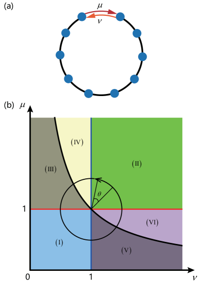
Figure 1: (a) Schematic of the model, which depicts a uniform tight-binding ring with unitary hopping strength, embedded by a single non-Hermitian dimer. It is an asymmetric tunneling with hopping strength $\mu$ and $\nu$. (b) Phase diagram of the system, which is consisted of six regions. In regions (I) and (II), system has full real spectrum, while in (III), (IV), (V) and (VI) the spectra are mixed with real and complex energy levels. At curve $\mu\nu=1$, all the energy levels are complex. The inset circle described by parameter equations $\nu=1+r\cos(\theta)$; $\mu=1+r\sin(\theta)$, goes through all six regions and will be used in the following figures.

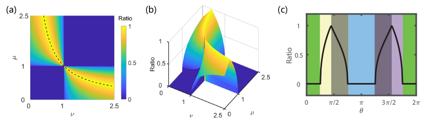
Figure 2: Plots of the ratio$\ g(\mu,\nu)$ in $\nu\mu$-plane from Eq. (14), as one of perspectives of the spectral statistics. (a) Color contour plot. The dished lines indicates the curve $\nu\mu=1$. The-nonanalytic behavior of $g(\mu,\nu)$ at lines $\mu\nu=1$ are obvious. (b) 3D plot. The nonanalytic behavior of $g(\mu,\nu)$ at curve $\mu\nu=1$ is highlighted. (c) Plots of the ratio at the loop $\nu=1+0.5\cos(\theta)$; $\mu=1+0.5\sin(\theta)$. The nonanalytic behaviors at the phase boundaries are clearly indicated by the sharp peaks and right angle turns.

Considering a simple uniform tight-binding ring, it is well known that the spectrum is cosine type and cannot be changed largely by a local impurity in general. An additional Hermitian hopping term or even non-Hermitian local on-site complex potential can only alter several energy levels, introducing localized states. However, we will see that another type of non-Hermitian impurity may have an affect on macroscopic energy levels, which plays the key role in the present work.

The Hamiltonian has the form

$$H=\sum\limits_{j=1}^{N-1}c_{j}^{{\dagger}}c_{j+1}+\mathrm{H.c.}+\mu c_{N}^{{\dagger}}c_{1}+\nu c_{1}^{{\dagger}}c_{N},$$ (1)

with odd $N/2$, where $c_{j}$ is the annihilation operator of fermion at site $j$. It depicts a uniform tight-binding ring with only a non-Hermitian impurity embedded. A schematic illustration of the model is presented in Fig. 1(a). The non-Hermiticity arises from an asymmetric tunneling between sites $1$ and $N$, represented by hopping strength $\mu$ and $\nu$ (in this paper, we only consider the case with $\mu,$ $\nu>0$ for simplicity). This model is investigated in the previous work WPPRA in the special case with $\mu\nu=1$. It has been shown that an asymmetric dimer can be realized by the combination of imaginary potential and magnetic flux LCPRA . Experiments on asymmetric dimer has been proposed Longhi ; LFengNC ; ZGong .

Unlike usual many-body non-Hermitian tight-binding model, Hamiltonian $H$ does not have parity-time symmetry and translational symmetry. Owing to the reality of the coupling $\mu$ and $\nu$, it possesses time reversal symmetry, ie., $\left[\mathcal{T},H\right]=0$, where $\mathcal{T}$ is an anti-unitary operator with action $\mathcal{T}^{-1}i\mathcal{T}=-i$. Fortunately, the solution of $H$ can be exactly obtained by the Bethe ansatz technique (see Appendix).

The Hamiltonian can be diagonalized as the form

$$H=\sum\limits_{n=1}^{N}\varepsilon_{n}\overline{\gamma}_{n}\gamma_{n}$$ (2)

where the fermion operators $\overline{\gamma}_{n}$ and $\gamma_{n}$ have the form

$$\overline{\gamma}_{n}=\sum_{l=1}^{N}f_{n}^{l}c_{l}^{{\dagger}},\gamma_{n}=\sum_{l=1}^{N}\overline{f_{n}^{l}}c_{l},$$ (3)

and satisfy the canonical commutative relation

$$\left\{\gamma_{m},\overline{\gamma}_{n}\right\}=\delta_{mn}.$$

Here the canonical conjugate operator can be constructed by the relation

$$\overline{f_{n}^{l}}(\mu,\nu)=\left[f_{n}^{l}(\nu,\mu)\right]^{\ast}$$ (4)

and the explicit expression of wave function is

$$\left\{\begin{array}[]{c}f_{n}^{l}=\frac{1}{\sqrt{\Omega}}\sin\left(k_{n}l+\alpha_{n}\right),(2<l<N-1)\\ f_{n}^{1}=\frac{1}{\sqrt{\Omega}},f_{n}^{N}=\frac{e^{-ik_{n}}-\mu e^{ik_{n}\left(N-1\right)}}{\nu-e^{ik_{n}N}}f_{1}\end{array}\right.$$ (5)

where $\alpha_{n}$ is obtained by $\tan\alpha_{n}=c_{n}/s_{n}$, and

$$s_{n} = \nu^{2}+1-\nu\cos\left(k_{n}N\right)+\nu\cos\left[k_{n}\left(N+2\right)\right]$$ (6)

$$-p_{n}\cos k_{n},$$

$$c_{n} = \nu\sin\left(k_{n}N\right)-\nu\sin\left[k_{n}\left(N+2\right)\right]+p_{n}\sin k_{n},$$ (7)

$$p_{n} = \cos\left[k_{n}\left(N+1\right)\right]-\mu\nu\cos\left[k_{n}\left(N-1\right)\right]$$ (8)

$$+\left(\mu+\nu\right)\cos k_{n}.$$

The coefficient $\Omega_{n}$ is determined by the biorthonormal inner product. In the rest of paper, we focus on the Dirac probability, since it can be measured directly in experiment. Then we take the Dirac normalization factor which is obtained from $\sum_{l=1}^{N}|f_{n}^{l}|^{2}=1$. The single-particle spectrum has the form

$$\varepsilon_{n}=e^{ik_{n}}+e^{-ik_{n}},$$ (9)

where $k_{n}$ can be real and complex. The quasi-wave vector $k_{n}$ for $1\leqslant n\leqslant N$ has the form

$$k_{n}=\frac{2n\pi}{N}+\theta_{n},$$ (10)

where $\theta_{n}$ is determined by the transcendental equations (see Appendix). The transcendental equation is reduced to

$$\tan\theta_{n}=\frac{\left(1-\mu\nu\right)\sin\left(\theta_{n}N\right)}{\mu+\nu-\left(1+\mu\nu\right)\cos\left(\theta_{n}N\right)},$$ (11)

for $n=N$ or $N/2$; and

$$\left\{\begin{array}[]{c}\sin(\phi_{n}+\theta_{n}N)=\frac{(\mu+\nu)\sin\frac{n\pi}{N}}{\sqrt{1+\mu^{2}\nu^{2}-2\mu\nu\cos\frac{2n\pi}{N}}}\\ \tan\phi_{n}=\frac{1+\mu\nu}{1-\mu\nu}\tan\frac{n\pi}{N}\end{array}\right.$$ (12)

otherwise. Obviously, the reality of $k_{n}$ ($1\leqslant n\leqslant N$) depends on the values of $\mu$ and $\nu$, which will be discussed in detail in the next section.

III Phase diagram

In this section, we analyze the property of the solution and the corresponding implications. At first, we determine the phase diagram from the perspective of spectral statistics, which is characterized by the proportion of the complex levels. Secondly, we introduce a concept, semi-localized state, to describe the feature of the eigenstates of complex energy levels. Furthermore, we reveal another exclusive property of the complex-level eigenstates, the non-steady, which only can be seen from an evolved (non-equilibrium) state in a Hermitian system.

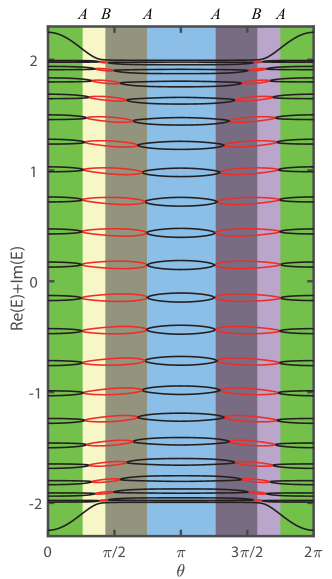
Figure 3: Plots of energy level structures for understanding the connection between the spectral statistics and QPTs. Energy levels for the system on the loop $\nu=1+0.9\cos(\theta)$; $\mu=1+0.9\sin(\theta)$ are plotted. Black and red lines represent the real and complex energy levels, respectively. There are two types of QPTs with the boundaries indicated by $A$ and $B$, respectively. We see that $A$-type boundary always corresponds to the appearance of complex levels, while $B$-type boundary locates at the maximal number of complex levels. The size of the system is $N=42$.

Figure 4: Schematic illustrations for the concept of semi-localized state. (a) Plots of the profiles of three kinds of wave functions: localized state (blue), extended state (yellow), and semi-localized state (red). The decay length of the semi-localized state has the same order of the lattice length. The dash lines represent the value of center of mass for each states. We see that a semi-localized state is a crossover between localized and extended states. (b) Plots of the probability current distributions for three kinds of states. The current for extended state and local state are both zero. The current distribution of a semi-localized state exhibits a non-steady behavior, violating the probability conservation, which is exclusive for the eigenstate of a non-Hermitian system. The size of the system is $N=150$. Other parameters are $\nu=5$, $\mu=10$ for the blue lines, $\nu=5$, $\mu=0.1$ for the red lines and $\nu=4$, $\mu=2$ for the yellow lines.

III.1 Spectral statistics

According to the solutions obtained in the Appendix, the reality of energy levels obeys the following rules. (i) $\mu,\nu>1$, or $\mu,\nu<1$, all the quasi-wave vectors $k_{n}$ are either real or imaginary, corresponding to real energy levels. All the eigenstates are non-degeneracy except the trivial case with $\mu=\nu=1$, which reduces the system to be a uniform Hermitian ring. We denote the (non-degeneracy) real-energy single-particle eigenstate as $\left|\psi_{\mathrm{R}}^{n}\right\rangle$, barring the energy levels $n=N$ and $N/2$. (ii) $\mu>1>\nu$, or $\mu<1<\nu$, some complex quasi-wave vectors $k_{n}$ appear, corresponding to complex energy levels, which come in pair with conjugate eigen energy. We denote the complex-energy single-particle eigenstate as $\left|\psi_{\mathrm{\pm}}^{n}\right\rangle$. (iii) Among them, especially in the case of $\mu\nu=1$, all $k_{n}$ becomes complex. Obviously, as one of the characteristics of the spectral statistics, the proportion of the complex level is defined as function of $\mu$ and $\nu$

$$g(\mu,\nu)=\frac{N_{\mathrm{C}}(\mu,\nu)}{N},$$ (13)

which is the ratio of the number of the complex levels $N_{\mathrm{C}}$ to the total number of levels. In large $N$ limit, we have

$$g(\mu,\nu)=\left\{\begin{array}[]{cc}0,&\mu,\nu\geqslant 1,\text{or }\mu,\nu\leqslant 1\\ (\pi-2k_{c})/\pi,&\mu>1>\nu,\text{or }\mu<1<\nu\\ 1,&\mu\nu=1\end{array}\right.,$$ (14)

where $k_{c}=|\arcsin[(1-\mu\nu)/(\nu-\mu)]|$ is the critical wave vector separating the real and complex levels. A schematic of the three kinds of regions, which will be shown as phase diagram is plotted in Fig. 1(b). To demonstrate the properties of the ratio, $3$D profiles of $g(\mu,\nu)$ and the corresponding energy-level structure are plotted in Fig. 2(a, b, c) and Fig. 3. We note that $g(\mu,\nu)$ is non-analytic at the curves $\mu=1$, $\nu=1$ and $\mu\nu=1$. We will show that such curves are phase boundaries for many-body ground state due to the sudden change of the spectral statistics.

III.2 Semi-localized state

Unlike a linear operator such as the parity, time reversal operator $\mathcal{T}$ is an anti-linear operator. The $\mathcal{T}$-symmetry breaking is always associated with the appearance of complex levels. Exact solution in Appendix shows that the single-particle eigen function can always be expressed to obey the relations

$$\mathcal{T}\left|\psi_{\mathrm{R}}^{n}\right\rangle=\left|\psi_{\mathrm{R}}^{n}\right\rangle,\text{ }\mathcal{T}\left|\psi_{\mathrm{\pm}}^{n}\right\rangle=\left|\psi_{\mathrm{\mp}}^{n}\right\rangle.$$ (15)

Owing to the value of $k_{n}$, there are three types of wave functions: extended, localized and semi-localized states. Here the last one is exclusive for non-Hermitian system. Unlike the localized one, the imaginary part of $k_{n}$ of semi-localized states, $\theta_{n}$ is inversely proportional to $N$, leading to an incomplete decay distribution (with a truncated tail). Nevertheless, it still supports imbalanced probability distribution, as a crossover from extended to localized states. We employ the center of mass (CoM), which is the expectation value of the CoM operator

$$r_{\mathrm{c}}=\frac{1}{N}\sum\limits_{l=1}^{N}lc_{l}^{{\dagger}}c_{l}.$$ (16)

Straightforward derivation shows that (i) $\left\langle r_{\mathrm{c}}\right\rangle\approx 1/2$ for an extended state; (ii) $\left\langle r_{\mathrm{c}}\right\rangle\approx 0$ ($1$) for a localized state at the case $\nu>\mu$ ($\mu>\nu$); and (iii) for a semi-localized state $\left\langle r_{\mathrm{c}}\right\rangle$ is a number ranging from $0$ to $1$. Here we give an example, when $\mu\nu=1$ and $\nu>1>\mu$, we have

$$\left\langle r_{c}\right\rangle\approx\frac{1}{(\sqrt[N]{\nu^{2}}-1)N}+\frac{1}{1-\nu^{2}},$$ (17)

in large $N$ limit. It is easy to check that $\lim_{\nu\rightarrow 1}\left\langle r_{c}\right\rangle=1/2$, which accords with the above analysis. To demonstrate the above conclusions, profiles of such three types of states and the corresponding $\left\langle r_{\mathrm{c}}\right\rangle$ are plotted in Fig. 4a. We can see that the difference among the three types of eigenstates is obvious.

III.3 Non-steady eigenstate

We note that the $\mathcal{T}$-symmetry breaking of $\left|\psi_{\mathrm{\pm}}^{n}\right\rangle$ indicates that $\left|\psi_{\mathrm{\pm}}^{n}\right\rangle$ can have non-zero local current, which is defined as

$$J_{l}=-i\left\langle\left(c_{l}^{{\dagger}}c_{l+1}-\mathrm{H.c.}\right)\right\rangle_{n},$$ (18)

at the position $l$. Here $\left\langle...\right\rangle_{n}$ denotes the expectation value for an eigenstate of $n$ level. It is usual for a Hermitian system, for instance, taking $\mu=\nu=1$, each eigenstate with nonzero momentum has zero local-current. Remarkably, an intriguing feature is that $\left|\psi_{\mathrm{\pm}}^{n}\right\rangle$ is a non-steady state, since $J_{l}$ is position-dependent, violating the conservation of current. A non-steady state can exist in a Hermitian system, such as a moving wavepacket in a tight-binding ring. However, it cannot be an eigenstate of a Hermitian system. If $\mu\leftrightarrows\nu$, the current changes the sign. In Fig. 4b, profiles of the current distributions for three types of eigenstates are plotted.

As a temporary summary, we can conclude that a semi-localized eigenstate has distinguishing feature from an extended one (The localized eigenstate can be negligible, since there are only two such eigenstates at most). This should result in macroscopic property for a many-body ground state.

IV Phase transition

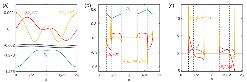
Figure 5: Plots of three quantities (a) density of ground state energy, (b) average CoM. (c) average staggered current, and the corresponding first-, second-order derivatives as function of $\theta$. It indicates that the density of groundstate energy does not display any critical behaviors, while the other two exhibit the characteristics of second-order QPT: first-order derivatives are non-analytical and second-order derivatives are divergent. The parameters are $\nu=1+0.9\cos(\theta)$; $\mu=1+0.9\sin(\theta)$. The size of the system is $N=750$.

Now we consider the many-body effect of the single-particle spectral statistics. We focus on the ground state for half-filled case, where all the negative real-parts of energy levels are filled by fermions. It is expected that the non-analyticity of $g(\mu,\nu)$ can result in macroscopic phenomena.

First of all, we consider the density of ground state energy, which is expressed as

$$E_{g}=\frac{2}{N}\sum\limits_{n=1}^{N/2}\varepsilon_{n}=\frac{2}{N}\sum\limits_{n=1}^{N/2}\text{{Re}}(\varepsilon_{n}).$$ (19)

From the exact result in the Appendix, $E_{g}$ is always analytical at all range of $\left\{\mu,\nu\right\}$, which seems to indicate that there is no occurrence of conventional QPT. Secondly, we investigate the average CoM, which is defined as

$$R_{\mathrm{c}}=\frac{2}{N}\sum\limits_{n=1}^{N/2}\left\langle r_{\mathrm{c}}\right\rangle_{n}.$$ (20)

From the exact result in the Appendix, we have

$$R_{\mathrm{c}}=\left\{\begin{array}[]{cc}1/2,&\mu,\nu>1,\text{or }\mu,\nu<1\\ 1/2+\eta(\mu,\nu),&\text{otherwise}\end{array}\right.$$ (21)

where $\eta(\mu,\nu)$ is a nonzero function. On the other hand, it is presumable that the non-analyticity of $g(\mu,\nu)$ at $\mu\nu=1$ can result in the non-analyticity of $R_{\mathrm{c}}$. Thirdly, we investigate the average staggered current, which is defined as

$$\mathcal{J}=-\frac{2i}{N}\sum\limits_{n=1}^{N/2}(-1)^{n}\langle\sum\limits_{l=2}^{N}\left(c_{l}^{{\dagger}}c_{l+1}-\mathrm{H.c.}\right)\rangle_{n}.$$ (22)

The feature of non-steady eigen states may also lead to non-analyticity of $\mathcal{J}(\mu,\nu)$ at the non-analytical point of $g(\mu,\nu)$. Actually we have

$$\mathcal{J}=\left\{\begin{array}[]{cc}0,&\mu,\nu\geqslant 1,\text{or }\mu,\nu\leqslant 1\\ \neq 0,&\text{otherwise}\\ 4/\pi,&\mu\nu=1\end{array}\right..$$ (23)

To demonstrate this point, we compute the quantities $\partial^{n}E_{g}/\partial\theta^{n}$, $\partial^{n}R_{\mathrm{c}}/\partial\theta^{n}$, and $\partial^{n}\mathcal{J}/\partial\theta^{n}$ along the circle

$$\nu=1+0.9\cos(\theta),\mu=1+0.9\sin(\theta)$$ (24)

with $n=1,2$. In Fig. 5, we plot these quantities from exact diagonalization results for finite size system. We find that the density of ground state energy does not display any critical behaviors as we predicted. It is different from a conventional QPT. It is understandable since the gound state does not experience a symmetry breaking as a whole, although a single-particle eigenstate has time-reversal symmetry breaking. However, the other two quantities exhibit the characteristics of second-order QPT: first-order derivatives are non-analytical and second-order derivatives are divergent.

V Conclusion

In summary we have proposed a new type of QPT beyond conventional symmetry-breaking and topological QPTs. It is based on the concept of semi-localization state, which is a crossover from extended to localized state, possessing exponentially decay probability distribution. The peculiar feature is that the decay length is of the order of the size of the system, rather than fixed as usual localized state. We have shown that such a semi-localized state can be induced by an asymmetrical dimer in a ring system. Remarkably, we found that a single dimer can result in a macroscopic amount of complex energy levels with semi-localized states, which determines the value of some macroscopic observables, such as the CoM and staggered current of the many-body ground state. Furthermore, the spectral statistics is non-analytical as asymmetrical hopping strengths vary, resulting in a sudden charge of the ground state, i.e., QPT. Another distinguishing feature of such a QPT is the groundstate energy is analytical at the phase boundary. The symmetry of the many-body ground state remains unchanged, while single-particle eigenstate breaks the time-reversal symmetry, resulting the formation of semi-localized state. It seems that such a quantum phase is exclusive for non-Hermitian system.

Appendix

In this Appendix, we present the detailed derivation and analysis for the Bethe Ansatz solution of the Hamiltonian $H$.

V.1 Wave function

We consider the single-particle eigen state

$$\left|\psi_{n}\right\rangle=\frac{1}{\sqrt{\Omega_{n}}}\sum_{l=1}^{N}f_{n}^{l}\left|l\right\rangle,$$ (25)

following a Bethe Ansatz form

$$f_{n}^{l}=\left\{\begin{array}[]{cc}1,&l=1\\ A_{n}e^{ik_{n}l}+B_{n}e^{-ik_{n}l},&l\in\left[2,N-1\right]\\ f_{n}^{N}&l=N\end{array}\right.,$$ (26)

where the normalization factor $\Omega_{n}=\sum_{n=1}^{N}|f_{n}^{l}|^{2}$ is determined by the Dirac inner product $\left\langle\psi_{k}\right.\left|\psi_{k}\right\rangle=1$. The Schrodinger equation

$$H\left|\psi_{n}\right\rangle=\varepsilon_{n}\left|\psi_{n}\right\rangle$$ (27)

with eigen energy $\varepsilon_{n}$, can be expressed in a explicit form

$$f_{n}^{l-1}+f_{n}^{l+1}=\varepsilon_{n}f_{n}^{l},$$ (28)

within the uniform region and

$$\left\{\begin{array}[]{l}f_{n}^{3}+f_{n}^{1}=\varepsilon_{n}f_{n}^{2}\\ f_{n}^{2}+\nu f_{n}^{N}=\varepsilon_{n}f_{n}^{1}\\ f_{n}^{N-1}+\mu f_{n}^{1}=\varepsilon_{n}f_{n}^{N}\\ f_{n}^{N-2}+f_{n}^{N}=\varepsilon_{n}f_{n}^{N-1}\end{array}\right.,$$ (29)

around the asymmetric dimer. Substituting Eq. (26) into Eqs. (28) and (29), we have

$$\varepsilon_{n}=2\cos k_{n},$$ (30)

and

$$\left\{\begin{array}[]{c}A_{n}e^{ik_{n}}+B_{n}e^{-ik_{n}}=f_{n}^{1}\\ A_{n}e^{2ik_{n}}+B_{n}e^{-2ik_{n}}=\varepsilon_{n}f_{n}^{1}-\nu f_{n}^{N}\\ A_{n}e^{ik_{n}\left(N-1\right)}+B_{n}e^{-ik_{n}\left(N-1\right)}=\varepsilon_{n}f_{N}-\mu f_{1}\\ A_{k}e^{ik_{n}N}+B_{k}e^{-ik_{n}N}=f_{N}\end{array}\right.,$$ (31)

the solution of Eq. (31) is

$$\left\{\begin{array}[]{c}A_{n}=\frac{1-\nu e^{-ik_{n}}f_{n}^{N}}{2i\sin k_{n}}=\frac{\mu-e^{-ik_{n}}f_{n}^{N}}{2i\sin k_{n}e^{ik_{n}N}}\\ B_{n}=\frac{\nu f_{n}^{N}e^{ik_{n}}-1}{2i\sin k_{n}}=\frac{e^{ik_{n}}f_{n}^{N}-\mu}{2i\sin k_{n}e^{-ik_{n}N}}\end{array}\right..$$ (32)

We would like to point out that the argument in the sine function can be complex number. We note that $A_{n}=(B_{n})^{\ast}$ if $k_{n}$ is real, which indicates the reality of the wave function, $f_{n}^{l}=\left(f_{n}^{l}\right)^{\ast}$, obeying the time-reversal symmetry. The existence of non-trivial solution $\left(A_{n},B_{n}\right)$ requires

$$\left(\mu+\nu\right)\sin k_{n}=\sin\left[k_{n}\left(1+N\right)\right]+\mu\nu\sin\left[k_{n}\left(1-N\right)\right].$$ (33)

And the solution of the wave function can be obtained from

$$\left\{\begin{array}[]{c}A_{n}=\frac{\nu-e^{ik_{n}N}-\nu e^{-2ik_{n}}+\mu\nu e^{ik_{n}\left(N-2\right)}}{2i\sin k_{n}\left(\nu-e^{ik_{n}N}\right)}\\ B_{n}=\frac{1-\mu\nu}{2i\sin k_{n}\left(\nu e^{-ik_{n}N}-1\right)}\end{array}\right.,$$ (34)

and

$$f_{n}^{N}=\frac{e^{-ik_{n}}-\mu e^{ik_{n}\left(N-1\right)}}{\nu-e^{ik_{n}N}}f_{1}.$$ (35)

In the following discussion, we use the normalized wave function

$$f_{n}^{l}=\sin\left(k_{n}l+\alpha_{n}\right),l\in\left[1,N\right]$$ (36)

by replacing $f_{n}^{l}$ by $\sqrt{\Omega_{n}}f_{n}^{l}$, where the coefficients are

$$\tan\alpha_{n}=\frac{c_{n}}{s_{n}},$$ (37)

$$s_{n} = \nu^{2}+1-\nu\cos\left(k_{n}N\right)+\nu\cos\left[k_{n}\left(N+2\right)\right]$$ (38)

$$-p_{n}\cos k_{n},$$

$$c_{n} = \nu\sin\left(k_{n}N\right)-\nu\sin\left[k_{n}\left(N+2\right)\right]+p_{n}\sin k_{n},$$

with

$$p_{n} = \cos\left[k_{n}\left(N+1\right)\right]-\mu\nu\cos\left[k_{n}\left(N-1\right)\right]$$ (39)

$$+\left(\mu+\nu\right)\cos k_{n}.$$

Similarly, the solution of $H^{{\dagger}}$ can be obtained as the form

$$\overline{f_{n}^{l}}(\mu,\nu)=\left[f_{n}^{l}(\nu,\mu)\right]^{\ast}$$ (40)

and obey the biorthonormal relation

$$\sum_{l}\overline{f_{m}^{l}}f_{n}^{l}=\delta_{mn}$$ (41)

if a biorthogonal inner product normalization factor is imposed.

Specifically, in the case with $\mu\nu=1$ and $\mu>1>\nu$ (or $\mu<1<\nu$), Eq. (33) reduces to

$$\sin\left[k_{n}\left(1+N\right)\right]+\sin\left[k_{n}\left(1-N\right)\right]-\left(\mu+\nu\right)\sin k_{n}=0,$$ (42)

and furthermore becomes

$$\cos\left(Nk_{n}\right)=\frac{\mu+\nu}{2}.$$ (43)

Since $(\mu+\nu)/2\geqslant 1$, we have

$$k_{n}=\frac{2n\pi}{N}+i\phi,$$ (44)

where $\phi=(\ln\nu)/N$. Equation (34) gives

$$\left\{\begin{array}[]{c}A_{k}=e^{-ik_{n}}\\ B_{k}=0\end{array}\right.,$$ (45)

so we have the wave function,

$$f_{l}=e^{i\frac{2n\pi}{N}l}e^{-\phi l},\text{ }l\in\left[1,N\right].$$ (46)

and the Dirac normalization factor

$$\Omega_{n}=\sum_{l=1}^{N}\left|f_{l}\right|^{2}=\frac{1-e^{-2\phi N}}{e^{2\phi}-1}.$$ (47)

V.2 Spectral statistics and phase diagram

Now we focus on the solution $k_{n}$ of the transcend equation in Eq. (33). Without loss of generality, taking

$$k_{n}=\frac{2n\pi}{N}+\theta_{n}.$$ (48)

For the general case ($n\neq N$ and $N/2$), Eq. (33) becomes

$$\sin\left(\phi_{n}+\theta_{n}N\right)=\sin\Theta_{n}$$ (49)

where

$$\tan\phi_{n}=\frac{1+\mu\nu}{1-\mu\nu}\tan\frac{2n\pi}{N}$$ (50)

and we define

$$\Theta_{n}=\arcsin\frac{\left(\mu+\nu\right)\sin\frac{2n\pi}{N}}{\sqrt{\left(1+\mu^{2}\nu^{2}\right)-2\mu\nu\cos\frac{4n\pi}{N}}}.$$ (51)

We notice that $\phi_{n}$ is always real. Then the complex $k_{n}$ arises from the complex $\theta_{n}$, leading to

$$\left|\frac{\left(\mu+\nu\right)\sin\frac{2n\pi}{N}}{\sqrt{\left(1+\mu^{2}\nu^{2}\right)-2\mu\nu\cos\frac{4n\pi}{N}}}\right|>1,$$ (52)

which is reduced to

$$\sin^{2}\frac{2n\pi}{N}>\frac{\left(\mu\nu-1\right)^{2}}{\left(\mu-\nu\right)^{2}}.$$ (53)

We find that the most fragile energy level is $n=N/4$, so the complex energy levels start to appear if

$$\left(1-\nu\right)\left(1-\mu\right)<0,$$ (54)

which is the appearance condition of the complex levels. The most stable energy level is $n=1$ or $N-1$, so all the $N-2$ energy levels turn to be complex at

$$\sin^{2}\frac{2\pi}{N}=\frac{\left(\mu\nu-1\right)^{2}}{\left(\mu-\nu\right)^{2}}.$$ (55)

We define the proportion of the complex level as the ratio

$$g(\mu,\nu)=\frac{N_{\mathrm{C}}(\mu,\nu)}{N}$$ (56)

where $N_{\mathrm{C}}$ is number of the complex levels. In large $N$ limit, $\sin^{2}(2\pi/N)\rightarrow 0$, then we have

$$g(\mu,\nu)=\left\{\begin{array}[]{cc}0,&\mu,\nu\geqslant 1,\text{or }\mu,\nu\leqslant 1\\ (\pi-2k_{c})/\pi,&\mu>1>\nu,\text{or }\mu<1<\nu\\ 1,&\mu\nu=1\end{array}\right.,$$ (57)

with $k_{c}=|\arcsin[(1-\mu\nu)/(\nu-\mu)]|$. This expression clearly shows that $g(\mu,\nu)$ is non-analytical at three curves $\mu=1$, $\nu=1$, and $\mu\nu=1$.

At last, for $n=N$ or $N/2$, Eq. (33) is reduced to

$$\tan\theta_{N}=\frac{\left(1-\mu\nu\right)\sin\left(\theta_{N}N\right)}{\mu+\nu-\left(1+\mu\nu\right)\cos\left(\theta_{N}N\right)}.$$ (58)

$\theta_{N}$ is either real for some configuration of ($\mu$, $\nu$) or complex with Re$\theta_{N}=\pi$ ($0$). For the second case, we take

$$\theta_{N}=\pi+i\epsilon\text{ or }i\epsilon,$$ (59)

which corresponds to real energy level but localized state. The decay rate and energy can be obtained from $\epsilon$, which obeys another transcend equation

$$\tan\left(i\phi\right)=\frac{\left(\mu\nu-1\right)\sin\left(Ni\epsilon\right)}{\left(1+\mu\nu\right)\cos\left(iN\epsilon\right)-\left(\mu+\nu\right)}.$$ (60)

V.3 Energy levels

Next we will show that for a fixed $n$, Eq. (49) must have a pair of solution $\left(\theta_{n},\overline{\theta}_{n}\right)$ leading to a pair of $(k_{n}$, $\overline{k}_{n})$. We will discuss it in the following cases.

(i) Real energy levels. In this case we have

$$\left\{\begin{array}[]{c}\theta_{n}N=\Theta_{n}-\phi_{n}\\ \overline{\theta}_{n}N=\pi-\Theta_{n}-\phi_{n}\end{array}\right.,$$ (61)

and accordingly

$$k_{n}=\frac{2n\pi}{N}+\theta_{n},\overline{k}_{n}=\frac{2n\pi}{N}+\overline{\theta}_{n},$$ (62)

for $n<N/2$. On the other hand, for the energy level $N-n$, we have

$$\tan\phi_{N-n}=-\frac{1+\mu\nu}{1-\mu\nu}\tan\frac{2n\pi}{N},$$ (63)

which means

$$\phi_{N-n}=2\pi-\phi_{n},$$ (64)

in comparison with Eq. (50). Furthermore, from

$$\sin\left(\phi_{N-n}+\theta_{N-n}N\right)=\sin\Theta_{N-n},$$ (65)

we get $\theta_{N-n}$ and $\overline{\theta}_{N-n}$ in the form of

$$\left\{\begin{array}[]{c}\theta_{N-n}N=\pi-\Theta_{N-n}-\phi_{N-n}=-\overline{\theta}_{n}N\\ \overline{\theta}_{N-n}N=2\pi+\Theta_{N-n}-\phi_{N-n}=-\theta_{n}N\end{array}\right.$$ (66)

and

$$\left\{\begin{array}[]{c}k_{N-n}=2\pi-\overline{k}_{n}\\ \overline{k}_{N-n}=2\pi-k_{n}\end{array}\right..$$ (67)

The corresponding energy levels satisfy $\varepsilon_{N-n}=\overline{\varepsilon}_{n}=2\cos\overline{k}_{n}$ and $\overline{\varepsilon}_{N-n}=\varepsilon_{n}=2\cos k_{n}$. In summary, if $k_{n}$ ($n<\frac{N}{2}$) is real and

$$k_{n}=\frac{1}{N}\left[2n\pi+\Theta_{n}-\phi_{n}\right],$$ (68)

with $\varepsilon_{n}$ there must exist another

$$k_{n^{\prime}}=\frac{1}{N}\left[(2n^{\prime}+1)\pi-\Theta_{n^{\prime}}-\phi_{n^{\prime}}\right],$$ (69)

with $n^{\prime}=N-n$ and $\varepsilon_{n^{\prime}}=\overline{\varepsilon}_{n}$. We see that $k_{n}$ is monotonic function except at the point $\mu=\nu=1$. Thus the real energy levels are non-degeneracy. The corresponding eigenstate has time reversal symmetry since the wave function is real.

(ii) Complex energy levels. In this case, we have $\sin(\phi_{n}+\theta_{n}N)>1$. The reality of $\sin(\phi_{n}+\theta_{n}N)$ requires that $\theta_{n}$ must be complex since $\phi_{n}$ is real. The two solutions of Eq. (49) are

$$\left\{\begin{array}[]{c}\theta_{n}N=\Theta_{n}-\phi_{n}\\ \overline{\theta}_{n}N=(\Theta_{n})^{\ast}-\phi_{n}\end{array}\right.,$$ (70)

and accordingly

$$\left\{\begin{array}[]{c}k_{n}=\frac{2n\pi}{N}+\theta_{n}\\ \overline{k}_{n}=\frac{2n\pi}{N}+\overline{\theta}_{n}\end{array}\right.,$$ (71)

the corresponding energy is $\varepsilon_{n}=2\cos(2n\pi/N+\theta_{n})$ and $\overline{\varepsilon}_{n}=2\cos(2n\pi/N+\overline{\theta}_{n})$. It indicates that

$$\overline{\varepsilon}_{n}=\left(\varepsilon_{n}\right)^{\ast}$$ (72)

i.e., the complex energy levels always come in pair. And two energy levels coalesce when $\theta_{n}=\overline{\theta}_{n}$. On the other hand, for the energy level $N-n$, we have

$$\phi_{N-n}=2\pi-\phi_{n}$$ (73)

which leads to

$$\left\{\begin{array}[]{c}\theta_{N-n}N=\Theta_{N-n}-\phi_{N-n}=-\theta_{n}N-2\pi\\ \overline{\theta}_{N-n}N=(\Theta_{N-n})^{\ast}-\phi_{N-n}=-\overline{\theta}_{n}N-2\pi\end{array}\right.,$$ (74)

and

$$\left\{\begin{array}[]{c}k_{N-n}=2\pi-k_{n}-\frac{2\pi}{N}\\ \overline{k}_{N-n}=2\pi-\overline{k}_{n}-\frac{2\pi}{N}\end{array}\right..$$ (75)

It indicates that the corresponding energy levels obey Im$k_{N-n}=\mathrm{Im}k_{n}=-\mathrm{Im}\overline{k}_{n}$, $\varepsilon_{N-n}\approx\varepsilon_{n}$, $\overline{\varepsilon}_{N-n}\approx\overline{\varepsilon}_{n}$ for large $N$ limit.

In summary, if $k_{n}$ ($n<\frac{N}{2}$) is complex and

$$k_{n}=\frac{1}{N}\left[2n\pi+\Theta_{n}-\phi_{n}\right],$$ (76)

with $\varepsilon_{n}$ there must exist another

$$k_{n^{\prime}}=\frac{1}{N}\left[2n^{\prime}\pi+(\Theta_{n^{\prime}})^{\ast}-\phi_{n^{\prime}}\right],$$ (77)

with $n^{\prime}=N-n$ and $\varepsilon_{n^{\prime}}=\overline{\varepsilon}_{n}$. We note that the corresponding eigen state breaks time reversal symmetry since the wave function is complex.

V.4 Center of mass

We still estimate the CoM in the following cases.

(i) Real energy levels. In this case, the eigenstate with real $k_{n}$ has the form

$$\left|\psi_{\mathrm{R}}^{n}\right\rangle=\frac{1}{\sqrt{\Omega_{n}}}\sum_{l=1}^{N}\sin\left(k_{n}l+\alpha_{n}\right)\left|l\right\rangle,$$ (78)

where

$$\alpha_{n}=\tan\frac{c_{n}}{s_{n}}$$

and $\Omega_{n}=\sum_{l=1}^{N}\sin^{2}\left(k_{n}l+\alpha_{n}\right)$ is Dirac normalization factor. Then the CoM of eigenstate $\left|\psi_{\mathrm{R}}^{n}\right\rangle$ is

$$\left\langle r_{c}^{\mathrm{R}}\right\rangle_{n} = \frac{1}{N}\sum\limits_{l=1}^{N}l\left\langle\psi_{\mathrm{R}}^{n}\right|c_{l}^{{\dagger}}c_{l}\left|\psi_{\mathrm{R}}^{n}\right\rangle$$ (79)

$$= \frac{1}{N\Omega_{n}}\sum_{l=1}^{N}l\sin^{2}\left(lk_{n}+\alpha_{n}\right).$$

Taking the approximation $k_{n}\approx 2n\pi/N$, together with the identities

$$\left\{\begin{array}[]{c}\sum_{l=1}^{N}l\sin^{2}\left(lk_{n}+\alpha_{n}\right)\approx\frac{N^{2}}{4}-\frac{N\sin\left(k_{n}+2\alpha_{n}\right)}{4\sin k_{n}}\\ \sum_{l=1}^{N}\sin^{2}\left(lk_{n}+\alpha_{n}\right)\approx\frac{N}{2}-\frac{\cos\left(\left(1+N\right)k_{n}+2\alpha_{n}\right)}{2\sin k_{n}\csc\left(k_{n}N\right)}\end{array}\right.,$$ (80)

we have

$$\left\langle r_{c}^{\mathrm{R}}\right\rangle_{n}\approx\frac{1}{2},$$ (81)

which shows that all $\left|\psi_{\mathrm{R}}^{n}\right\rangle$ have the same CoM, locating at the center of the lattice.

(ii) Complex energy levels. In this case, the eigenstates of conjugate pair are expressed as

$$\left|\psi_{\mathrm{+}}^{n}\right\rangle = \frac{1}{\sqrt{\Omega_{n}}}\sum_{l=1}^{N}\sin\left(k_{n}l+\alpha_{n}\right)\left|l\right\rangle,$$ (82)

$$\left|\psi_{\mathrm{-}}^{n}\right\rangle = \frac{1}{\sqrt{\Omega_{n}}}\sum_{l=1}^{N}\sin\left(k_{n}^{\ast}l+\alpha_{n}^{\ast}\right)\left|l\right\rangle.$$ (83)

Similarly, the corresponding CoMs, defined as

$$\left\langle r_{c}^{\mathrm{\pm}}\right\rangle_{n}=\frac{1}{N}\sum\limits_{l=1}^{N}l\left\langle\psi_{\mathrm{\pm}}\right|c_{l}^{{\dagger}}c_{l}\left|\psi_{\mathrm{\pm}}\right\rangle$$ (84)

are identical with each other

$$\left\langle r_{c}^{\mathrm{+}}\right\rangle_{n}=\left\langle r_{c}^{\mathrm{-}}\right\rangle_{n}=\left\langle r_{c}\right\rangle_{n}$$ (85)

since $\left|\psi_{\mathrm{+}}^{n}\right\rangle\$and $\left|\psi_{\mathrm{-}}^{n}\right\rangle\$have the same distributions of Dirac probability. According to Eq. (36), we have

$$\sum_{l=1}^{N}\left|\sin\left(k_{n}l+\alpha_{n}\right)\right|^{2}$$ (86)

$$\approx \frac{1}{2}\cosh(k_{\text{{I}}}+k_{\text{{I}}}N+2\alpha_{\text{{I}}})\text{{csch}}(k_{\text{{I}}})\sinh(k_{\text{{I}}}N)$$

and

$$\sum_{l=1}^{N}l\left|\sin\left(k_{n}l+\alpha_{n}\right)\right|^{2}$$ (87)

$$\approx \frac{1}{8}\text{{csch}}^{2}k_{n}^{\text{{I}}}(\cosh 2\alpha_{n}^{\text{{I}}}-\left(1+N\right)\cosh[2(k_{n}^{\text{{I}}}N+\alpha_{n}^{\text{{I}}})]$$

$$+N\cosh[2(k_{n}^{\text{{I}}}+k_{n}^{\text{{I}}}N+\alpha_{n}^{\text{{I}}})]),$$

where

$$k_{n}^{\text{{R}}} = \text{{Re}}k_{n}\text{, }k_{n}^{\text{{I}}}=\text{{Im}}k_{n}\text{,}$$ (88)

$$\alpha_{n}^{\text{{R}}} = \text{{Re}}\alpha_{n}\text{, }\alpha_{n}^{\text{{I}}}=\text{{Im}}\alpha_{n}\text{.}$$

Finally we get

$$\left\langle r_{c}\right\rangle_{n}\approx\frac{N^{-1}\cosh\left(2\alpha_{n}^{\text{{I}}}\right)-\cosh[2(k_{n}^{\text{{I}}}N+\alpha_{n}^{\text{{I}}})]+\cosh[2(k_{n}^{\text{{I}}}+k_{n}^{\text{{I}}}N+\alpha_{n}^{\text{{I}}})]}{4\cosh(k_{n}^{\text{{I}}}+k_{n}^{\text{{I}}}N+2\alpha_{n}^{\text{{I}}})\sinh(k_{n}^{\text{{I}}}N)\sinh(k_{n}^{\text{{I}}})}$$ (89)

which indicates that the CoM of complex level has distribution from $0$ to $1$.

For the special case with $\mu\nu=1$, and $\mu>1>\nu$ $($or $\mu<1<\nu)$, it readily to obtain

$$\left\langle r_{c}\right\rangle_{n}\approx\frac{1}{(\sqrt[N]{\nu^{2}}-1)N}+\frac{1}{1-\nu^{2}}$$ (90)

in large $N$ limit, which is independent of $n$.

V.5 Current

We now turn to the current of eigenstate, which is defined as

$$J_{l}^{n} = -i\left\langle\left(c_{l}^{\dagger}c_{l+1}-\mathrm{H.c.}\right)\right\rangle_{n}$$

$$= -i(\left(f_{n}^{l}\right)^{\ast}f_{n}^{l+1}-\left(f_{n}^{l+1}\right)^{\ast}f_{n}^{l}).$$

According to Eq. (36), for the eigenstates with real $k_{n}$, we always have

$$J_{l}^{n}=0.$$ (92)

In contrast, for the eigenstates with complex $k_{n}$, we have

$$J_{l}^{n} = -i(\sin\left(k_{n}^{\ast}l+\alpha_{n}^{\ast}\right)\sin\left(k_{n}l+\alpha_{n}+k_{n}\right)$$

$$-\sin\left(k_{n}^{\ast}l+k_{n}^{\ast}+\alpha_{n}^{\ast}\right)\sin\left(k_{n}l+\alpha_{n}\right)).$$

Taking a trigonometric transformation and an approximation $\sinh(k_{n}^{\text{{I}}})\approx 0$, one can obtain

$$J_{l}^{n}\approx-\sin(k_{n}^{\text{{R}}})\sinh(2k_{n}^{\text{{I}}}l+2\alpha_{n}^{\text{{I}}}+k_{n}^{\text{{I}}}).$$

We see that the current with $k_{n}^{\ast}$ is $\left(J_{l}^{n}\right)^{\ast}=-J_{l}^{n}$, i.e., the sum current of a conjugate pair always vanishes. We introduce the concept of the average staggered current,

$$\mathcal{J}=-\frac{2i}{N}\sum\limits_{n=1}^{N/2}(-1)^{n}\langle\sum\limits_{l=2}^{N}\left(c_{l}^{{\dagger}}c_{l+1}-\mathrm{H.c.}\right)\rangle_{n},$$ (94)

which is nonzero for the band containing complex levels. A direct derivation yields

$$\langle\sum\limits_{l=2}^{N}\left(c_{l}^{{\dagger}}c_{l+1}-\mathrm{H.c.}\right)\rangle_{n}$$

$$= -i\sin(k_{n}^{\text{{R}}})\text{{csch}}(k_{n}^{\text{{I}}})\sinh(k_{n}^{\text{{I}}}N)\sinh(2k_{n}^{\text{{I}}}+2\alpha_{n}^{\text{{I}}}+Nk_{n}^{\text{{I}}}).$$

for large $N$. The average staggered current has the from

$$\mathcal{J} = -\frac{2}{N}\sum\limits_{n=1}^{N/2}(-1)^{n}\sin(k_{n}^{\text{{R}}})\text{{csch}}(k_{n}^{\text{{I}}})$$ (96)

$$\times\sinh(k_{n}^{\text{{I}}}N)\sinh(2k_{n}^{\text{{I}}}+2\alpha_{n}^{\text{{I}}}+Nk_{n}^{\text{{I}}}).$$

For the special case with $\mu\nu=1$, in large $N$ limit, it readily to obtain

$$\mathcal{J}\approx\frac{4}{\pi}.$$ (97)

In summary, we have

$$\mathcal{J}=\left\{\begin{array}[]{cc}0,&\mu,\nu\geqslant 1,\text{or }\mu,\nu\leqslant 1\\ \neq 0,&\text{otherwise}\\ 4/\pi,&\mu\nu=1\end{array}\right.,$$ (98)

which has the implication that $\mathcal{J}$ can characterize the phase transitions.

References

- (1) S. Sachdev, Quantum Phase Transitions (Cambridge University Press, Cambridge, England, 1999).
- (2) X. L. Qi, Y. S. Wu, and S. C. Zhang, Topological quantization of the spin hall effect in two-dimensional paramagnetic semiconductors, Phys. Rev. B 74, 085308 (2006).
- (3) M. Znojil, Conditional observability, Phys. Lett. B 650, 440 (2007).
- (4) M. Znojil, Tridiagonal PT-symmetric N-by-N Hamiltonians and a fine-tuning of their observability domains in the strongly non-Hermitian regime, J. Phys. A 40, 13131 (2007).
- (5) O. Bendix, R. Fleischmann, T. Kottos, and B. Shapiro, Exponentially Fragile Symmetry in Lattices with Localized Eigenmodes, Phys. Rev. Lett. 103, 030402 (2009).
- (6) S. Longhi, Bloch Oscillations in Complex Crystals with Symmetry, Phys. Rev. Lett. 103, 123601 (2009).
- (7) S. Longhi, Dynamic localization and transport in complex crystals, Phys. Rev. B 80, 235102 (2009).
- (8) L. Jin and Z. Song, Solutions of symmetric tight-binding chain and its equivalent Hermitian counterpart, Phys. Rev. A 80, 052107 (2009).
- (9) M. Znojil, Gegenbauer-solvable quantum chain model, Phys. Rev. A 82, 052113 (2010).
- (10) S. Longhi, Bloch oscillations in tight-binding lattices with defects, Phys. Rev. B 81, 195118 (2010).
- (11) S. Longhi, Periodic wave packet reconstruction in truncated tight-binding lattices, Phys. Rev. B 82, 041106(R) (2010).
- (12) L. Jin and Z. Song, Physics counterpart of the non-Hermitian tight-binding chain, Phys. Rev. A 81, 032109 (2010).
- (13) Y. N. Joglekar, D. Scott, M. Babbey, and A. Saxena, Robust and fragile -symmetric phases in a tight-binding chain, Phys. Rev. A 82, 030103(R) (2010).
- (14) M. Znojil, An exactly solvable quantum-lattice model with a tunable degree of nonlocality, J. Phys. A 44, 075302 (2011).
- (15) M. Znojil, The crypto-Hermitian smeared-coordinate representation of wave functions, Phys. Lett. A 375, 3176 (2011).
- (16) H. Zhong, W. Hai, G. Lu, and Z. Li, Incoherent control in a non-Hermitian Bose-Hubbard dimer, Phys. Rev. A 84, 013410 (2011).
- (17) L. B. Drissi, E. H. Saidi, and M. Bousmina, Graphene, Lattice Field Theory and Symmetries, J. Math. Phys. 52, 022306 (2011).
- (18) Y. N. Joglekar and A. Saxena, Robust -symmetric chain and properties of its Hermitian counterpart, Phys. Rev. A 83, 050101(R) (2011).
- (19) D. D. Scott and Y. N. Joglekar, Degrees and signatures of broken -symmetry in nonuniform lattices, Phys. Rev. A 83, 050102(R) (2011).
- (20) Y. N. Joglekar and J. L. Barnett, Origin of maximal symmetry breaking in even -symmetric lattices, Phys. Rev. A 84, 024103 (2011).
- (21) D. D. Scott and Y. N. Joglekar, -symmetry breaking and ubiquitous maximal chirality in a -symmetric ring, Phys. Rev. A 85, 062105 (2012).
- (22) T. E. Lee and Y. N. Joglekar, -symmetric Rabi model: Perturbation theory, Phys. Rev. A 92, 042103 (2015).
- (23) M. Kulishov et al, Nonreciprocal waveguide Bragg gratings, Opt. Express 13, 3068 (2005).
- (24) S. Longhi, Transparency in Bragg scattering and phase conjugation, Opt. Lett. 35, 3844 (2010).
- (25) Z. Lin, H. Ramezani, T. Eichelkraut, T. Kottos, H. Cao, and D. N. Christodoulides, Unidirectional Invisibility Induced by -Symmetric Periodic Structures, Phys. Rev. Lett. 106, 213901 (2011).
- (26) A. Regensburger, C. Bersch, M. Ali Miri, G. Onishchukov, D. N. Christodoulides, and U. Peschel, Parity-time synthetic photonic lattices, Nature (London) 488, 167 (2012).
- (27) T. Eichelkraut et al, Mobility transition from ballistic to diffusive transport in non-Hermitian lattices, Nat. Commun. 4, 2533 (2013).
- (28) L. Feng et al, Experimental demonstration of a unidirectional reflectionless parity-time metamaterial at optical frequencies, Nat. Mater. 12, 108 (2013).
- (29) B. Peng et al, Parity–time-symmetric whispering-gallery microcavities, Nat. Phys. 10, 394 (2014).
- (30) L. Chang, et al, Parity-time symmetry and variable optical isolation in active-passive-coupled microresonators, Nat. Photonics 8, 524 (2014).
- (31) S. Longhi, Invisibility in non-Hermitian tight-binding lattices, Phys. Rev. A 82, 032111 (2010).
- (32) S. Longhi and G. Della Valle, Invisible defects in complex crystals, Ann. Phys. (NY) 334, 35 (2013).
- (33) X. Z. Zhang and Z. Song, Momentum-independent reflectionless transmission in the non-Hermitian time-reversal symmetric system, Ann. Phys. (NY) 339, 109 (2013).
- (34) Y. Sun, W. Tan, H. Q. Li, J. Li, and H. Chen, Experimental Demonstration of a Coherent Perfect Absorber with Phase Transition, Phys. Rev. Lett. 112, 143903 (2014).
- (35) A. Mostafazadeh, Spectral Singularities of Complex Scattering Potentials and Infinite Reflection and Transmission Coefficients at Real Energies, Phys. Rev. Lett. 102, 220402 (2009).
- (36) S. Longhi, Spectral singularities in a non-Hermitian Friedrichs-Fano-Anderson model, Phys. Rev. B 80, 165125 (2009).
- (37) X. Z. Zhang, L. Jin, and Z. Song, Self-sustained emission in semi-infinite non-Hermitian systems at the exceptional point, Phys. Rev. A 87, 042118 (2013).
- (38) S. Longhi, Half-spectral unidirectional invisibility in non-Hermitian periodic optical structures, Opt. Lett. 40, 5694 (2015).
- (39) X. Q. Li, X. Z. Zhang, G. Zhang, and Z. Song, Asymmetric transmission through a flux-controlled non-Hermitian scattering center, Phys. Rev. A 91, 032101 (2015).
- (40) B. Peng et al, Loss-induced suppression and revival of lasing, Science 346, 328 (2014).
- (41) L. Feng, Z. J. Wong, R. M. Ma, Y. Wang, and X. Zhang, Single-mode laser by parity-time symmetry breaking, Science 346, 972 (2014).
- (42) H. Hodaei, M. A. Miri, M. Heinrich, D. N. Christodoulides, and M. Khajavikhan, Tunable Parity-Time-Symmetric Microring Lasers, Science 346, 975 (2014).
- (43) L. Jin and Z. Song, Incident Direction Independent Wave Propagation and Unidirectional Lasing, Phys. Rev. Lett. 121, 073901 (2018).
- (44) C. Li, G. Zhang, X. Z. Zhang, and Z. Song, Conventional quantum phase transition driven by a complex parameter in a non-Hermitian PT-symmetric Ising model. Phys. Rev. A 90, 012103 (2014).
- (45) C. Li and Z. Song, Finite-temperature quantum criticality in a complex-parameter plane, Phys. Rev. A 92, 062103 (2015).
- (46) C. Li, G. Zhang, and Z. Song, Chern number in Ising models with spatially modulated real and complex fields, Phys. Rev. A 94, 052113 (2016).
- (47) C. Li, X. Z. Zhang, G. Zhang, and Z. Song, Topological phases in a Kitaev chain with imbalanced pairing, Phys. Rev. B 97, 115436 (2018).
- (48) R. Wang, X. Z. Zhang, Z. Song, Dynamical topological invariant for the non-Hermitian Rice-Mele model, Phys. Rev. A 98, 042120 (2018).
- (49) S. Lin, L. Jin, and Z. Song, Symmetry protected topological phases characterized by isolated exceptional points, Phys. Rev. B 99, 165148 (2019).
- (50) L. Jin and Z. Song, Bulk-boundary correspondence in a non-Hermitian system in one dimension with chiral inversion symmetry, Phys. Rev. B 99, 081103(R) (2019).
- (51) X. Z. Zhang and Z. Song, Partial topological Zak phase and dynamical confinement in a non-Hermitian bipartite system, Phys. Rev. A 99, 012113 (2019).
- (52) K. L. Zhang, H. C. Wu, L. Jin, and Z. Song, Topological phase transition independent of system non-Hermiticity, Phys. Rev. B 100, 045141 (2019).
- (53) C. M. Bender, Making sense of non-Hermitian Hamiltonians, Rep. Prog. Phys. 70, 947 (2007).
- (54) Z. H. Musslimani, K. G. Makris, R. El-Ganainy, and D. N. Christodoulides, Optical Solitons in PT Periodic Potentials, Phys. Rev. Lett. 100, 030402 (2008).
- (55) K. G. Makris, R. El-Ganainy, D. N. Christodoulides, and Z. H. Musslimani, Beam Dynamics in PT Symmetric Optical Lattices, Phys. Rev. Lett. 100, 103904 (2008).
- (56) S. Klaiman, U. Günther, and N. Moiseyev, Visualization of Branch Points in PT-Symmetric Waveguides, Phys. Rev. Lett. 101, 080402 (2008).
- (57) C. E. Rüter et al., Observation of parity-time symmetry in optics, Nat. Phys. 6, 192 (2010).
- (58) Y. D. Chong, L. Ge, H. Cao, and A. D. Stone, Coherent perfect absorbers: time-reversed lasers, Phys. Rev. Lett. 105, 053901 (2010).
- (59) L. Feng et al., Experimental demonstration of a unidirectional reflectionless parity-time metamaterial at optical frequencies, Nature Mater. 12, 108 (2013).
- (60) R. Fleury, D. Sounas, and A. Alù, An invisible acoustic sensor based on parity-time symmetry, Nat. Commun. 6, 5905 (2015).
- (61) C. M. Bender, Making sense of non-Hermitian Hamiltonians, Rep. Prog. Phys. 70, 947 (2007).
- (62) N. Moiseyev, Non-Hermitian Quantum Mechanics (Cambridge Univ. Press, 2011).
- (63) L. Feng, R. El-Ganainy, and L. Ge, Non-Hermitian photonics based on parity–time symmetry, Nat. Photo. 11, 752 (2017).
- (64) R. El-Ganainy, K. G. Makris, M. Khajavikhan, Z. H. Musslimani, S. Rotter, and D. N. Christodoulides, Non-Hermitian physics and PT symmetry, Nat. Phys. 14, 11 (2018).
- (65) S. K. Gupta, Y. Zou, X. Y. Zhu, M. H. Lu, L. Zhang, X. P. Liu, and Y. F. Chen, Parity-time Symmetry in Non-Hermitian Complex Media, arXiv:1803.00794.
- (66) D. Christodoulides and J. Yang, Parity-time Symmetry and Its Applications (Springer, 2018).
- (67) P. Wang, Z. Song, and L. Jin, Non-Hermitian phase transition and eigenstate localization induced by asymmetric coupling, Phys. Rev. A 99, 062112 (2019).
- (68) C. Li, L. Jin, and Z. Song, Non-Hermitian interferometer: Unidirectional amplification without distortion, Phys. Rev. A 95, 022125 (2017).
- (69) S. Longhi, D. Gatti, and G. Della Valle, Sci. Rep. 5, 13376 (2015); Phys. Rev. B 92, 094204 (2015).
- (70) B. Midya, H. Zhao, and L. Feng, Nat. Commun. 9, 2674 (2018).
- (71) Z. P. Gong, Y. Ashida, K. Kawabata, K. Takasan, S. Higashikawa, and M. Ueda, Phys. Rev. X 8, 031079 (2018).