Waiting time distributions in a two-level fluctuator coupled to
a superconducting charge detector
Abstract
We analyze charge fluctuations in a parasitic state strongly coupled to a superconducting Josephson-junction-based charge detector. The charge dynamics of the state resembles that of electron transport in a quantum dot with two charge states, and hence we refer to it as a two-level fluctuator. By constructing the distribution of waiting times from the measured detector signal and comparing it with a waiting time theory, we extract the electron in- and out-tunneling rates for the two-level fluctuator, which are severely asymmetric.
I Introduction
Parasitic states including charge traps are present in almost all solid-state devices and there has been several proposals on how to avoid them. Holweg et al. (1992); Galperin et al. (1994); Galperin and Chao (1995); Keijsers et al. (1996); Balkashin et al. (1998); Oh et al. (2006); Schriefl et al. (2006); Zimmerman et al. (2008); Burnett et al. (2014) Two-level fluctuators (TLFs), for example, substantially affect qubit coherence time Möttönen et al. (2006); Ku and Yu (2005); Müller et al. (2009); Goetz et al. (2016) and degrade charge sensingGiblin et al. (2016). However, if the time scales of charge fluctuations in a trap are significantly different from those of the operation of the actual device, their harmful effect can be mitigated. In silicon, TLFs have been characterized by various approaches using metallic single-electron transistors Zimmerman et al. (1997); Furlan and Lotkhov (2003); Sun and Kane (2009); Pourkabirian et al. (2014); Zimmerman et al. (2008), a scheme to which we contribute in this paper.
Electron waiting times have been investigated for a wide range of physical systems including quantum dots, Brandes (2008); Welack et al. (2008, 2009); Welack and Yan (2009); Thomas and Flindt (2013); Tang et al. (2014); Tang and Wang (2014); Sothmann (2014); Talbo et al. (2015); Rudge and Kosov (2016a, b); Ptaszyński (2017); Rudge and Kosov (2018); Stegmann et al. (2018); Kleinherbers et al. (2018); Tang et al. (2018); Rudge and Kosov (2019) coherent conductors, Albert et al. (2012); Haack et al. (2014) molecular junctions Seoane Souto et al. (2015); Kosov (2018), and superconducting systems. Rajabi et al. (2013); Dambach et al. (2015, 2016); Albert et al. (2016); Chevallier et al. (2016); Walldorf et al. (2018); Mi et al. (2018) Distributions of waiting times contain complementary information on charge transport properties which is not necessarily encoded in the full counting statistics (FCS) and vice versa Brandes (2008). For example, waiting-time distributions capture the interference effects in double-dot setups Welack et al. (2008), reveal the correlations in multichannel systems Tang et al. (2014); Dasenbrook et al. (2015), allow to separate slow and fast dynamics in Cooper-pair splitters Walldorf et al. (2018), resolve few-photon processes Brange et al. (2019), and even investigate the topological superconductivity in hybrid junctions Mi et al. (2018). In dynamic, periodically driven systems, waiting-time distributions are clear indicators of regular single-electron transport Albert et al. (2011); Dasenbrook et al. (2014); Potanina and Flindt (2017); Burset et al. (2019). Furthermore, waiting-time distributions were used in a recent experiment Gorman et al. (2017) to optimize single-electron spin-readout fidelity.
In this work, we investigate electronic waiting times between charge transitions in and out of a parasitic state to directly extract the time-scales of such TLF. We employ a superconducting single-electron transistor (SSET) to monitor the switching events on the TLF and apply a continuous electrostatic feedback on the detector to maintain a constant charge sensitivity, which tends to fasten an asymmetry in the detected in- and out-tunneling rates.
This paper is organized as follows: In Sec. II, we provide a short overview of the waiting time theory Brandes (2008) and illustrate these concepts by evaluating the distribution of electron waiting times for a TLF in Secs. II.1 and II.2. We treat the two-level fluctuator as a potential well that is in tunnel contact with a charge reservoir as illustrated in in Fig. 1(a). In Sec. III, we discuss our experimental setup. In Sec. IV we present our measurement results and compare them with the waiting-time-distribution theory. Since our model assumes sequential in- and out-tunneling, we calculate the FCS of the switching events and compare the results with the waiting times. Finally, in Sec. V, we conclude our work.
II Electron waiting times
The time that passes between two subsequent single-electron tunneling events of the same type is usually referred to as the electron waiting time .Brandes (2008); Albert et al. (2011, 2012) The single-electron tunneling process has a stochastic nature and therefore is described by a waiting-time distribution (WTD) function . For stationary Markovian transport problems, the WTD relates to the idle-time probability as Albert et al. (2012); Haack et al. (2014)
| (1) |
where is the probability of having no tunneling events during a time span . The mean waiting time can be expressed in terms of the idle-time probability asAlbert et al. (2012); Haack et al. (2014) .
The statistics of single-electron tunneling events is captured by the probability of having tunneling events of the chosen type during the time span .Bagrets and Nazarov (2003); Flindt et al. (2008, 2010) However, we only need to know the idle-time probability to obtain the WTD. In FCS, the moment generating function
| (2) |
provides us with all the moments of as . From Eq. (2) we observe that is exactly the idle-time probability. Next, we utilize these concepts by evaluating the WTDs for a two-level fluctuator.
II.1 Waiting times in a two-level fluctuator
We describe the parasitic state as a single-electron box consisting of a nano-scale island, the charge dynamics of which is governed by the master equation
| (3) |
where the vector contains the probabilities and for the island to be empty or occupied by electron, respectively, and the rate matrix describes the transitions between and charge states of the island.
We partition the rate matrix as with jump operators describing charge transfers to and from the island, respectively Benito et al. (2016). We resolve the probability vector such that it accounts for the number of tunneling events . The -resolved equations of motion, , are decoupled by introducing the counting field via the definition . We then arrive at a modified master equation for
| (4) |
For in Eq. (4), we recover the original master equation (3). Further on, we focus on the waiting times between the into-the-island tunneling events, and hence set . In this case, the modified rate matrix assumes the form
| (5) |
We have included the counting factor in the lower off-diagonal element together with , corresponding to counting the number of tunneling events into the parasitic state.Bagrets and Nazarov (2003); Flindt et al. (2008, 2010) The solution of the modified master equation formally reads:
| (6) |
The idle-time probability follows as , where is an th component of the vector . For a given rate matrix (5) the solution is analytic and we are able to evaluate the WTD for a two-level fluctuator using relation (1) as
| (7) |
where is the waiting time between single-electron subsequent tunneling events from the charge reservoir to the parasitic state. We continue with another example of WTD, where we take into account the effect of finite detection time.
II.2 Residence times in a two-level fluctuator coupled to a detector
Let us focus on the time that the electron spends in the parasitic state known as the residence time Talkner et al. (2005). We use the term residence time to avoid confusion with the waiting time discussed in the previous section. When the residence time becomes comparable to the inverse of the detector bandwidth, , we have to take it into account when evaluating the distribution of residence times.
Due to the finite bandwidth of the detector, we may fail to detect some of the tunneling events. Therefore, we add two more possible states when formulating the rate equation.Naaman and Aumentado (2006) The revised probability vector reads . Probabilities and correspond to the situation when parasitic state is empty or occupied, respectively, but it has not been detected. The detected empty and occupied states are denoted by and , respectively.
While actual charge transitions between the occupied state to the undetected empty state may occur several times before the empty state gets detected, we obtain the experimentally observed residence time distribution by counting the events . After including the effect of the finite detector bandwidth in the rate equation, we arrive at the following rate matrix Gustavsson et al. (2007); Flindt et al. (2009):
| (8) |
In analogy to the previous section, we solve the modified rate equation given the rate matrix Eq. (8) and obtain the idle-time probability . We evaluate the detected residence time distribution using double differentiation as and obtain
| (9) |
where and . If we assume the detector to be perfect , we recover the exponential decay of the occupied parasitic state .
III Experimental setup
We employ a superconducting charge detector which consists of two Al/Al2O3/Al Josephson junctions in series with resistances and capacitances , , and a superconducting gap , which form a charge island with a charging energy of , where , is the elementary charge, is the capacitive coupling between the gate and the island, and is the mutual capacitance between the TLF and the detector island. The device is fabricated on a 500-m-thick high-resistivity silicon wafer with 5-nm-thick high-purity field oxide. The measurements are carried out in a cryostat that has a base temperature of mK. Figure 1(b) shows the top view of a detector that is nominally identical to the device that is used to carry out the presented experiments. The Al leads provide galvanic contacts between the tunnel junctions and the gate voltage is used to tune the charge sensitivity of the SSET. The bias voltage controls the electrochemical potential of the lead, whereas the other lead is connected to a room temperature transimpedance amplifier. At the output port of the amplifier, we measure the voltage and transmit the signal to a proportional-integral-derivative (PID) feedback circuit that maintains the gate charge point, and hence the charge sensitivity of the detector.
The charge stability of the detector, shown in Fig. 1(c), reveals how to associate the measured dc current with the gate-tunable charge point of the superconducting island. To minimize the detector backaction on the two-level fluctuator, we choose the bias voltage that corresponds to the double-Josephson-quasiparticle processClerk et al. (2002); Xue et al. (2009).
IV Results
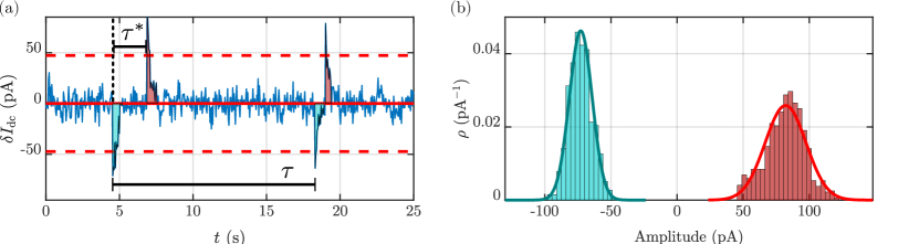
The signal produced by the TLF is read out using the detector such that the PID controller is utilized and tuned to a setpoint near the highest sensitivity. In addition to the white noise, we observe a systematic signal, as exemplified in Fig. 2(a). The jumps are distinguished from the white noise when the amplitude of the detector signal exceeds the 5 white-noise level. Furthermore, the detector signal is filtered with a two-point moving averaging window, which results in a detector bandwidth of Hz.
First, a jump with a negative sign appears and the detector current offset takes a negative value. Then, the PID steers back to the setpoint using the detector gate. After residence time, another jump appears, but always with the opposite, positive sign compared to the first jump. The consecutive jump occurs at counted from the previous negative jump. The probability distribution of the jump amplitudes, shown in Fig. 2(b), seems Gaussian, however the mean values and variances are different for the different jump directions.
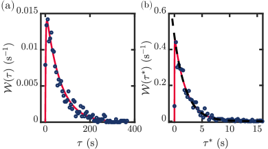
Since the switching between the two states is associated with single-electron transitions, and can be extracted from traces such as that shown in Fig. 2(a). The total duration of the measured time trace is 16 h that provides approximately 1000 back-and-forth tunneling events, giving rise to the WTD shown in Fig. 3(a).
We obtain the parameters and by fitting Eq. (7) to the data in Fig. 3(a). The fitted waiting-time distribution, where the tunneling rates are s-1 and s-1, agrees well with the measured distribution. The significant difference between and originate from the energy splitting of the two charge states and from the feedback; for every switching event the detector gate induces a compensating electrostatic field that not only affects the operation of the SSET, but also tends to polarize the TLF towards the opposite state. Since the average residence time is significantly shorter than and comparable to , we fit Eq. (9) to the residence time distribution, shown in Fig. 3(b), by first fixing and according to the WTD. Thus, the only fitting parameter in the model is , with the estimated Hz based on the fit. The fitted deviates roughly 7.6% from the nominal detector bandwidth.
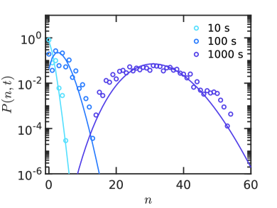
From the measured state transitions we can also construct the counting statistics used in Eq. (2), where denotes the number of switching events regardless of the direction. The limited number of total jumps requires a moving time window to achieve the FCS with different of the time window lengths. Therefore, consecutive time windows are shifted by 1 s and used in the average over the 16-h time trace. The Markovian single-electron tunnelling in a dot coupled to a charge reservoir follows the Poisson distributionMaisi et al. (2014). If we assume an effective tunneling rate , we can fit a Poisson distribution to the data shown in Fig. 4. The extracted effective tunneling rate is s-1, which can be explained by the branching of jumps observed in Fig. 2(a). More precisely, we effectively observe two events with a rate of , since after each in-tunneling event there is an out-tunneling event with a brief delay.
V Conclusions
We have demonstrated that WTD is useful in extracting the time scales of a TLF. Including the finite bandwidth of the detector in the waiting-time theory provides us with an accurate distribution of the waiting times in the charge trap. In contrast to WTD, full counting statistics covers long time scales and delivers mean values, noise, and high-order moments. Both approaches are powerful tools and they are connected Brandes (2008). From the observed probability distribution , we conclude that charge transitions in the TLF constitute a Poisson process. The distribution of waiting times, Eq. (7), indicates that there are two Poisson processes with different rates and in the two-level fluctuator. It requires less steps to evaluate the WTD than to evaluate the full counting statistics . Moreover, the waiting-time formalism allows to evaluate the WTD analytically where as an analytic expression for is not currently available. Waiting times belong to the short-time-scale statistics and are sensitive to the finite detector bandwidth. Here, we have shown how the distribution of waiting times has obvious advantages in extracting the short time scales of the system.
Acknowledgements.
E.P. thanks C. Flindt for helpful comments. This work was carried out as part of the Academy of Finland Centre of Excellence program 312300 and grants 308161, 314302, and 316551. E.P. acknowledges support from the Vilho, Yrjö and Kalle Foundation of the Finnish Academy of Science and Letters through the grant for doctoral studies. We acknowledge the provision of facilities and technical support by Aalto University at OtaNano - Micronova and the NSW Node of the Australian National Fabrication Facility, where the devices were fabricated. We acknowledge funding from the Joint Research Project ‘e-SI-Amp’ (15SIB08) and the Australian Research Council (DP160104923). This project has received funding from the European Metrology Programme for Innovation and Research (EMPIR) co-financed by the Participating States and from the European Union Horizon 2020 research and innovation programme.References
- Holweg et al. (1992) P. A. M. Holweg, J. Caro, A. H. Verbruggen, and S. Radelaar, “Ballistic electron transport and two-level resistance fluctuations in noble-metal nanobridges,” Phys. Rev. B 45, 9311 (1992).
- Galperin et al. (1994) Yu. M. Galperin, Nanzhi Zou, and K. A. Chao, “Resonant tunneling in the presence of a two-level fluctuator: Average transparency,” Phys. Rev. B 49, 13728 (1994).
- Galperin and Chao (1995) Yu. M. Galperin and K. A. Chao, “Resonant tunneling in the presence of a two-level fluctuator: Low-frequency noise,” Phys. Rev. B 52, 12126 (1995).
- Keijsers et al. (1996) R. J. P. Keijsers, O. I. Shklyarevskii, and H. van Kempen, “Point-Contact Study of Fast and Slow Two-Level Fluctuators in Metallic Glasses,” Phys. Rev. Lett. 77, 3411 (1996).
- Balkashin et al. (1998) O. P. Balkashin, R. J. P. Keijsers, H. van Kempen, Yu. A. Kolesnichenko, and O. I. Shklyarevskii, “Relaxation of two-level fluctuators in point contacts,” Phys. Rev. B 58, 1294 (1998).
- Oh et al. (2006) S. Oh, K. Cicak, J. S. Kline, M. A. Sillanpää, K. D. Osborn, J. D. Whittaker, R. W. Simmonds, and D. P. Pappas, “Elimination of two level fluctuators in superconducting quantum bits by an epitaxial tunnel barrier,” Phys. Rev. B 74, 100502 (2006).
- Schriefl et al. (2006) J. Schriefl, Y. Makhlin, A. Shnirman, and G. Schön, “Decoherence from ensembles of two-level fluctuators,” N. J. Phys. 8, 1 (2006).
- Zimmerman et al. (2008) N. M. Zimmerman, W. H. Huber, B. Simonds, E. Hourdakis, A. Fujiwara, Y.i Ono, Y. Takahashi, H. Inokawa, M. Furlan, and M. W. Keller, “Why the long-term charge offset drift in Si single-electron tunneling transistors is much smaller (better) than in metal-based ones: Two-level fluctuator stability,” J. Appl. Phys. 104, 033710 (2008).
- Burnett et al. (2014) J. Burnett, L. Faoro, I. Wisby, V. L. Gurtovoi, A. V. Chernykh, G. M. Mikhailov, V. A. Tulin, R. Shaikhaidarov, V. Antonov, P. J. Meeson, A. Ya Tzalenchuk, and T. Lindström, “Evidence for interacting two-level systems from the 1/f noise of a superconducting resonator,” Nat. Commun. 5, 4119 (2014), article.
- Möttönen et al. (2006) M. Möttönen, R. de Sousa, J. Zhang, and K. B. Whaley, “High-fidelity one-qubit operations under random telegraph noise,” Phys. Rev. A 73, 022332 (2006).
- Ku and Yu (2005) L.-C. Ku and C. C. Yu, “Decoherence of a Josephson qubit due to coupling to two-level systems,” Phys. Rev. B 72, 024526 (2005).
- Müller et al. (2009) C. Müller, A. Shnirman, and Y. Makhlin, “Relaxation of Josephson qubits due to strong coupling to two-level systems,” Phys. Rev. B 80, 134517 (2009).
- Goetz et al. (2016) J. Goetz, F. Deppe, M. Haeberlein, F. Wulschner, C. W. Zollitsch, Sebastian Meier, M. Fischer, P. Eder, E. Xie, K. G. Fedorov, E. P. Menzel, A. Marx, and R. Gross, “Loss mechanisms in superconducting thin film microwave resonators,” J. Appl. Phys. 119, 015304 (2016).
- Giblin et al. (2016) S. P. Giblin, P. See, A. Petrie, T. J. B. M. Janssen, I. Farrer, J. P. Griffiths, G. A. C. Jones, D. A. Ritchie, and M. Kataoka, “High-resolution error detection in the capture process of a single-electron pump,” Applied Physics Letters 108, 023502 (2016).
- Zimmerman et al. (1997) N. M. Zimmerman, J. L. Cobb, and A. F. Clark, “Modulation of the charge of a single-electron transistor by distant defects,” Phys. Rev. B 56, 7675 (1997).
- Furlan and Lotkhov (2003) M. Furlan and S. V. Lotkhov, “Electrometry on charge traps with a single-electron transistor,” Phys. Rev. B 67, 205313 (2003).
- Sun and Kane (2009) L. Sun and B. E. Kane, “Detection of a single-charge defect in a metal-oxide-semiconductor structure using vertically coupled Al and Si single-electron transistors,” Phys. Rev. B 80, 153310 (2009).
- Pourkabirian et al. (2014) A. Pourkabirian, M. V. Gustafsson, G. Johansson, J. Clarke, and P. Delsing, “Nonequilibrium Probing of Two-Level Charge Fluctuators Using the Step Response of a Single-Electron Transistor,” Phys. Rev. Lett. 113, 256801 (2014).
- Brandes (2008) T. Brandes, “Waiting times and noise in single particle transport,” Ann. Phys. 17, 477 (2008).
- Welack et al. (2008) S. Welack, M. Esposito, U. Harbola, and S. Mukamel, “Interference effects in the counting statistics of electron transfers through a double quantum dot,” Phys. Rev. B 77, 195315 (2008).
- Welack et al. (2009) S. Welack, S. Mukamel, and Y. J. Yan, “Waiting time distributions of electron transfers through quantum dot Aharonov-Bohm interferometers,” Europhys. Lett. 85, 57008 (2009).
- Welack and Yan (2009) S. Welack and Y. J. Yan, “Non-Markovian theory for the waiting time distributions of single electron transfers,” J. Chem. Phys. 131, 114111 (2009).
- Thomas and Flindt (2013) K. H. Thomas and C. Flindt, “Electron waiting times in non-Markovian quantum transport,” Phys. Rev. B 87, 121405 (2013).
- Tang et al. (2014) G.-M. Tang, F. Xu, and J. Wang, “Waiting time distribution of quantum electronic transport in the transient regime,” Phys. Rev. B 89, 205310 (2014).
- Tang and Wang (2014) G.-M. Tang and J. Wang, “Full-counting statistics of charge and spin transport in the transient regime: A nonequilibrium Green’s function approach,” Phys. Rev. B 90, 195422 (2014).
- Sothmann (2014) B. Sothmann, “Electronic waiting-time distribution of a quantum-dot spin valve,” Phys. Rev. B 90, 155315 (2014).
- Talbo et al. (2015) V. Talbo, J. Mateos, S. Retailleau, P. Dollfus, and T. González, “Time-dependent shot noise in multi-level quantum dot-based single-electron devices,” Semicond. Sci. Technol. 30, 055002 (2015).
- Rudge and Kosov (2016a) S. L. Rudge and D. S. Kosov, “Distribution of residence times as a marker to distinguish different pathways for quantum transport,” Phys. Rev. E 94, 042134 (2016a).
- Rudge and Kosov (2016b) S. L. Rudge and D. S. Kosov, “Distribution of tunnelling times for quantum electron transport,” J. Chem. Phys. 144, 124105 (2016b).
- Ptaszyński (2017) K. Ptaszyński, “Nonrenewal statistics in transport through quantum dots,” Phys. Rev. B 95, 045306 (2017).
- Rudge and Kosov (2018) S. L. Rudge and D. S. Kosov, “Distribution of waiting times between electron cotunneling events,” Phys. Rev. B 98, 245402 (2018).
- Stegmann et al. (2018) P. Stegmann, J. König, and S. Weiss, “Coherent dynamics in stochastic systems revealed by full counting statistics,” Phys. Rev. B 98, 035409 (2018).
- Kleinherbers et al. (2018) E. Kleinherbers, P Stegmann, and P König, “Revealing attractive electron–electron interaction in a quantum dot by full counting statistics,” New J. Phys. 20, 073023 (2018).
- Tang et al. (2018) G. Tang, F. Xu, S. Mi, and J. Wang, “Spin-resolved electron waiting times in a quantum-dot spin valve,” Phys. Rev. B 97, 165407 (2018).
- Rudge and Kosov (2019) S. L. Rudge and D. S. Kosov, “Nonrenewal statistics in quantum transport from the perspective of first-passage and waiting time distributions,” Phys. Rev. B 99, 115426 (2019).
- Albert et al. (2012) M. Albert, G. Haack, C. Flindt, and M. Büttiker, “Electron Waiting Times in Mesoscopic Conductors,” Phys. Rev. Lett. 108, 186806 (2012).
- Haack et al. (2014) G. Haack, M. Albert, and C. Flindt, “Distributions of electron waiting times in quantum-coherent conductors,” Phys. Rev. B 90, 205429 (2014).
- Seoane Souto et al. (2015) R. Seoane Souto, R. Avriller, R. C. Monreal, A. Martín-Rodero, and A. Levy Yeyati, “Transient dynamics and waiting time distribution of molecular junctions in the polaronic regime,” Phys. Rev. B 92, 125435 (2015).
- Kosov (2018) D. S. Kosov, “Waiting time between charging and discharging processes in molecular junctions,” J. Chem. Phys. 149, 164105 (2018).
- Rajabi et al. (2013) L. Rajabi, C. Pöltl, and M. Governale, “Waiting Time Distributions for the Transport through a Quantum-Dot Tunnel Coupled to One Normal and One Superconducting Lead,” Phys. Rev. Lett. 111, 067002 (2013).
- Dambach et al. (2015) S. Dambach, B. Kubala, V. Gramich, and J. Ankerhold, “Time-resolved statistics of nonclassical light in Josephson photonics,” Phys. Rev. B 92, 054508 (2015).
- Dambach et al. (2016) S. Dambach, B. Kubala, and J. Ankerhold, “Time-resolved statistics of photon pairs in two-cavity Josephson photonics,” Fortschr. Phys. , 1 (2016).
- Albert et al. (2016) M. Albert, D. Chevallier, and P. Devillard, “Waiting times of entangled electrons in normal–-superconducting junctions,” Physica E 76, 215 (2016).
- Chevallier et al. (2016) D. Chevallier, M. Albert, and P. Devillard, “Probing Majorana and Andreev bound states with waiting times,” Europhys. Lett. 116, 27005 (2016).
- Walldorf et al. (2018) N. Walldorf, C. Padurariu, A.-P. Jauho, and C. Flindt, “Electron Waiting Times of a Cooper Pair Splitter,” Phys. Rev. Lett. 120, 087701 (2018).
- Mi et al. (2018) S. Mi, P. Burset, and C. Flindt, “Electron waiting times in hybrid junctions with topological superconductors,” Sci. Rep. 8, 16828 (2018).
- Dasenbrook et al. (2015) D. Dasenbrook, P. P. Hofer, and C. Flindt, “Electron waiting times in coherent conductors are correlated,” Phys. Rev. B 91, 195420 (2015).
- Brange et al. (2019) F. Brange, P. Menczel, and C. Flindt, “Photon counting statistics of a microwave cavity,” Phys. Rev. B 99, 085418 (2019).
- Albert et al. (2011) M. Albert, C. Flindt, and M. Büttiker, “Distributions of Waiting Times of Dynamic Single-Electron Emitters,” Phys. Rev. Lett. 107, 086805 (2011).
- Dasenbrook et al. (2014) D. Dasenbrook, C. Flindt, and M. Büttiker, “Floquet Theory of Electron Waiting Times in Quantum-Coherent Conductors,” Phys. Rev. Lett. 112, 146801 (2014).
- Potanina and Flindt (2017) E. Potanina and C. Flindt, “Electron waiting times of a periodically driven single-electron turnstile,” Phys. Rev. B 96, 045420 (2017).
- Burset et al. (2019) P. Burset, J. Kotilahti, M. Moskalets, and C. Flindt, “Time-Domain Spectroscopy of Mesoscopic Conductors Using Voltage Pulses,” Adv. Quantum Technol. 2, 1970023 (2019).
- Gorman et al. (2017) S. K. Gorman, Y. He, M. G. House, J. G. Keizer, D. Keith, L. Fricke, S. J. Hile, M. A. Broome, and M. Y. Simmons, “Tunneling statistics for analysis of spin-readout fidelity,” Phys. Rev. Appl. 8, 034019 (2017).
- Bagrets and Nazarov (2003) D. A. Bagrets and Yu. V. Nazarov, “Full counting statistics of charge transfer in Coulomb blockade systems,” Phys. Rev. B 67, 085316 (2003).
- Flindt et al. (2008) C. Flindt, T. Novotný, A. Braggio, M. Sassetti, and A.-P. Jauho, “Counting Statistics of Non-Markovian Quantum Stochastic Processes,” Phys. Rev. Lett. 100, 150601 (2008).
- Flindt et al. (2010) C. Flindt, T. Novotný, A. Braggio, and A.-P. Jauho, “Counting statistics of transport through Coulomb blockade nanostructures: High-order cumulants and non-Markovian effects,” Phys. Rev. B 82, 155407 (2010).
- Benito et al. (2016) M. Benito, M. Niklas, and S. Kohler, “Full-counting statistics of time-dependent conductors,” Phys. Rev. B 94, 195433 (2016).
- Talkner et al. (2005) P. Talkner, Ł. Machura, M. Schindler, P. Hänggi, and J. Łuczka, “Statistics of transition times, phase diffusion and synchronization in periodically driven bistable systems,” New J. Phys. 7, 14 (2005).
- Naaman and Aumentado (2006) O. Naaman and J. Aumentado, “Poisson transition rates from time-domain measurements with a finite bandwidth,” Phys. Rev. Lett. 96, 100201 (2006).
- Gustavsson et al. (2007) S. Gustavsson, R. Leturcq, T. Ihn, K. Ensslin, M. Reinwald, and W. Wegscheider, “Measurements of higher-order noise correlations in a quantum dot with a finite bandwidth detector,” Phys. Rev. B 75, 075314 (2007).
- Flindt et al. (2009) C. Flindt, C. Fricke, F. Hohls, T. Novotny, K. Netocny, T. Brandes, and R. J. Haug, “Universal oscillations in counting statistics,” Proc. Natl. Acad. Sci. 106, 10116 (2009).
- Clerk et al. (2002) A. A. Clerk, S. M. Girvin, A. K. Nguyen, and A. D. Stone, “Resonant Cooper-pair tunneling: Quantum noise and measurement characteristics,” Phys. Rev. Lett. 89, 176804 (2002).
- Xue et al. (2009) W. W. Xue, Z. Ji, Feng Pan, Joel Stettenheim, M. P. Blencowe, and A. J. Rimberg, “Measurement of quantum noise in a single-electron transistor near the quantum limit,” Nat. Phys. 5, 660–664 (2009).
- Maisi et al. (2014) V. F. Maisi, D. Kambly, C. Flindt, and J. P. Pekola, “Full counting statistics of Andreev tunneling,” Phys. Rev. Lett. 112, 036801 (2014).