Greybody Factor for a Rotating Bardeen Black Hole

M. Sharif and Qanitah Ama-Tul-Mughani
Department of Mathematics, University of the Punjab,
Quaid-e-Azam Campus, Lahore-54590, Pakistan
msharif.math@pu.edu.pkqanitah94@gmail.com
Abstract

In this paper, we formulate an analytical expression of greybody factor in the context of rotating Bardeen black hole which is valid in low energy and low angular momentum region. Primarily, we analyze the profile of effective potential which originates the absorption probability. We then derive two asymptotic solutions by solving the radial part of Klein-Gordon equation in two different regions, namely, black hole and far-field horizons. We match these solutions smoothly to an intermediate regime to extend our results over the whole radial coordinate. In order to elaborate the significance of analytical solution, we compute the energy emission rate and absorption cross-section for the massless scalar field. It is found that the rotation parameter increases the emission rate of scalar field particles while the orbital angular momentum minimizes the emission process.

Keywords: Black hole; Greybody factor; Klein-Gordon equation.
PACS: 04.70.Dy; 52.25.Tx.

1 Introduction

Black holes (BHs) are the most mysterious and abstruse astronomical objects as they have singularities covered by the event horizons. In general relativity, singularity is a region where all laws of physics break down and gravitational pull diverges in this region of spacetime. To avoid these undefined regions, a set of solutions dubbed as “regular BHs” have played an essential role to overcome this obstacle which do not have any singularity even at the origin. In literature, the first ever regular spherically symmetric BH solution was obtained by Bardeen [1], known as Bardeen BH. As the Bardeen BH was not a vacuum solution, therefore a special form of the energy-momentum tensor was introduced to attain the model satisfying the weak energy bounds. After that, characteristics of such regular BH solutions have extensively been carried out in general relativity [2]-[7].

Newman and Janis [8] applied a complex coordinate transformation on Schwarzschild solution to obtain a regular as well as rotating BH solution without using the field equations. Ay$\acute{o}$n-Beato and Garc$\acute{i}$a [9] reinterpreted the Bardeen model as the magnetic solution of field equations coupled with nonlinear electrodynamics. Drake and Szekeres [10] generated the Kerr-Newman metric, representing a rotating charged BH, by applying Newman-Janis scheme on the Reissner-Nordstr$\ddot{o}$m metric. Bambi and Modesto [11] used this algorithm to the regular Hayward and Bardeen BH metrics to construct a family of rotating BH spacetimes.

Classically, it is accepted that BH absorbs everything from its surrounding due to strong gravitational effects and does not emit any type of radiations as well as particles. However, it has been shown that BHs can create and discharge thermal radiations by taking into account the quantum mechanical effects. In the gravitational context, these thermal emissions named as Hawking radiation [12] gradually lead to decrease in the BH mass and finally to its eventual evaporation. It is believed that any primordial BH having mass less than $10^{15}$g would have disappeared by now. Black holes as thermal objects associate entropy and Hawking temperature which vary for different class of BHs [13]-[15]. The emission process at the horizon of BH, in terms of frequency, is given as [12]

$$\gamma(w)=\left(\frac{d^{3}k}{e^{\frac{w}{T_{H}}}(2\pi)^{3}}\right),$$

where $T_{H}$ is the Hawking temperature. This expression can be modified up to any dimensions and valid for massless as well as massive particles. Consequently, the radiation spectrum at the horizon is exactly equal to the black body spectrum which gives rise to loss of information paradox. The inevitable reality is that the spacetime around a BH is nontrivial which alters the spectra of Hawking radiation by allowing some of the radiations to cross the barrier and rest of them reflect back to BH.

The greybody factor (rate of absorption probability) is defined as the probability for an incoming wave from infinity to be absorbed by the BH which is directly related to absorption cross-section [16]-[20]. The relation between emission rate and greybody factor can be expressed as

$$\gamma(w)=\left(\frac{|\tilde{\emph{A}}_{l,m}|^{2}d^{3}k}{e^{\frac{w}{T_{H}}}(2\pi)^{3}}\right),$$

where $|\tilde{\emph{A}}_{l,m}|^{2}$ depicts the greybody factor which is also a frequency dependent quantity. Creek et al. [21, 22] studied the scalar emission rate for rotating BH and derived both numerical as well as analytical solutions for the greybody factor. Boonserm et al. [23] computed some rigorous bounds on the greybody factors associated with scalar field excitations for the Myers-Perry BH. Jorge et al. [24] explored the greybody factors in low frequency regime for higher dimensional rotating BHs with the cosmological constant being zero, positive or negative. Toshmatov et al. [25] investigated the absorption probability for regular BH spacetimes and observed that charge parameter decreases the transmission rate of the incident wave. Ahmed and Saifullah [26] computed the greybody factor for uncharged scalar particles in the background of cylindrically symmetric spacetime and found an analytical solution in the form of hypergeometric function. Dey and Chakrabarti [27] evaluated the quasinormal modes as well as absorption probability for the Bardeen-de Sitter BH due to gravitational perturbation. Recently, Hyun et al. [28] found an analytical expression of greybody factor for the brane scalar field in five-dimensional rotating BH by using spheroidal joining factor.

In this paper, we derive an analytical solution of absorption probability for rotating Bardeen BH. The paper is organized as follows. In section 2, we evaluate effective potential through the decoupled set of radial and angular equations resulting from the Klein-Gordon equation. Section 3 leads to two asymptotic solutions by solving the radial equation of motion at two different horizons. We also calculate the energy emission rate and absorption cross-section for the massless scalar field. The last section concludes our results.

2 Klein-Gordon Equation and Effective Potential

The axially symmetric spacetime for rotating Bardeen BH in Boyer-Lindquist coordinates is given as

$$ds^{2}=-F(r,\theta)dt^{2}+\frac{1}{G(r,\theta)}dr^{2}+\Sigma(r,\theta)d\theta^{2}+H(r,\theta)d\phi^{2}-2K(r,\theta)dtd\phi,$$ (1)

where

$\displaystyle F(r,\theta)$ $\displaystyle=$ $\displaystyle\frac{\Pi(r)-a_{0}^{2}\sin^{2}\theta}{\Sigma(r,\theta)},\quad G(r,\theta)=\frac{\Pi(r)}{\Sigma(r,\theta)},\quad\Sigma(r,\theta)=r^{2}+a_{0}^{2}\cos^{2}\theta,$
$\displaystyle H(r,\theta)$ $\displaystyle=$ $\displaystyle\frac{\sin^{2}\theta\left((r^{2}+a_{0}^{2})^{2}-\Pi(r)a_{0}^{2}\sin^{2}\theta\right)}{\Sigma(r,\theta)},\quad\Pi(r)=r^{2}+a_{0}^{2}-2rM(r),$
$\displaystyle K(r,\theta)$ $\displaystyle=$ $\displaystyle\frac{a_{0}\sin^{2}\theta(r^{2}+a_{0}^{2}-\Pi(r))}{\Sigma(r,\theta)},$

$a_{0}$ represents the rotation parameter while the mass function is defined as

$$M(r)=M_{0}\left(\frac{r^{3}}{(r^{2}+r_{0}^{2})^{\frac{3}{2}}}\right).$$

Here, $M_{0}$ corresponds to the mass of BH and $r_{0}$ as length parameter, measures the deviation of considered class of BH from the Kerr geometry [11]. Moreover, it is noted that curvature invariants, i.e., Ricci and Kretschmann scalars are regular (bounded and non-singular) everywhere even at the origin, hence we can name the line element (1) as rotating Bardeen regular BH. Through computing $R_{\mu\nu}$ and $T_{\mu\nu}$, Azreg-Ainou [29] found that the spacetime (1) satisfies the field equations. The event horizons are evaluated by the condition

$$\Pi(r)=0=r^{2}-2rM(r)+a_{0}^{2}.$$ (2)

In order to calculate the analytic expression of greybody factor, we first derive the equation of motion to examine the propagation of scalar field. We presume that particles are only minimally coupled to gravity and do not involve in any other interaction. In this scenario, the equation of motion takes the form

$$\nabla_{\mu}\nabla^{\mu}\Psi=\partial_{\mu}[\sqrt{-g}g^{\mu\nu}\partial_{\nu}\Psi(t,r,\theta,\phi)]=0,$$ (3)

which, through Eq.(1) and $\sqrt{-g}=-\frac{\Sigma(K^{2}+FH)}{G}$, turns out to be

$\displaystyle\sqrt{-g}\left(\frac{-H}{K^{2}+FH}\right)\partial_{tt}\Psi+2\sqrt{-g}\left(\frac{-K}{K^{2}+FH}\right)\partial_{t}\partial_{\phi}\Psi+\sqrt{-g}\left(\frac{F}{K^{2}+FH}\right)\partial_{\phi\phi}\Psi$
$\displaystyle+(\sqrt{-g}G\partial_{r}\Psi)_{,r}+(\sqrt{-g}\frac{1}{\Sigma}\partial_{\theta}\Psi)_{,\theta}=0.$ (4)

For separation of variables, the field factorization

$$\Psi(t,r,\theta,\phi)=\exp(-\iota wt)\exp(\iota m\phi)R_{wlm}(r)S^{m}_{l}(\theta,a_{0}w),$$

where $S^{m}_{l}(\theta,a_{0}w)$ are angular spheroidal functions [30, 31], leads to the following decoupled set of radial and angular equations

$\displaystyle\frac{\partial}{\partial r}(\Pi\frac{\partial R_{wlm}}{\partial r})+\left[\frac{1}{\Pi}((w^{2}(r^{2}+a_{0}^{2})^{2}-a_{0}^{2})-a_{0}^{2}m^{2}-4a_{0}rM)-\lambda_{l}^{m}\right]R_{wlm}=0,$
(5)
$\displaystyle\frac{1}{\sin\theta}\frac{\partial}{\partial\theta}\left(\sin\theta\frac{\partial S^{m}_{l}}{\partial\theta}\right)+(\frac{m^{2}}{\sin^{2}\theta}-w^{2}a_{0}^{2}\sin^{2}\theta+\lambda_{l}^{m})S^{m}_{l}(\theta,a_{0}w)=0.$ (6)

Here $\lambda_{l}^{m}$ is a separation constant which establishes a connection between decoupled equations.

In general, the separation constant cannot be expressed in a closed form. However, its analytic expression can be obtained as a power series in terms of parameter $a_{0}w$ [32, 33] given as

$$\lambda_{l}^{m}=\sum_{n=0}^{\infty}\textit{f}_{~{}n}^{~{}lm}(a_{0}w)^{n}.$$ (7)

For the purpose of simplicity, we truncate the series and only keep the terms up to third order which is expressed as follows

$$\lambda_{l}^{m}=l(l+1)+\frac{-2m^{2}+2l(l+1)-1}{(2l-1)(2l+3)}(a_{0}w)^{2}+O((a_{0}w)^{4}),$$ (8)

with $\textit{f}_{~{}1}^{~{}lm}=\textit{f}_{~{}3}^{~{}lm}=0$. Here, the parameter $l$ denotes the orbital angular momentum with non-negative integeral values satisfying $l\geq|m|$ and $\frac{l-|m|}{2}\in\{0,\mathbb{Z}^{+}\}$. Now, we are in a position to solve the radial equation (5) analytically by using the above mentioned power series expression. The obtained solution will lead us to determine the greybody factor for a massless scalar field. Before computing greybody factor, we analyze the profile of effective potential which is responsible to originate it. Introducing a new radial mode transformation

$$R_{wlm}(r)=\frac{U_{wlm}(r)}{\sqrt{r^{2}+a_{0}^{2}}},$$ (9)

and tortoise coordinate $x_{*}$

$$\frac{dx_{*}}{dr}=\frac{r^{2}+a_{0}^{2}}{\Pi(r)},$$ (10)

such that

$$\frac{d}{dx_{*}}=\frac{\Pi(r)}{r^{2}+a_{0}^{2}}\frac{d}{dr},\quad\frac{d^{2}}{dx_{*}^{2}}=\left(\frac{\Pi(r)}{r^{2}+a_{0}^{2}}\right)^{2}\frac{d^{2}}{dr^{2}}+\left(\frac{\Pi(r)}{r^{2}+a_{0}^{2}}\right)\frac{d}{dr}\left(\frac{\Pi(r)}{r^{2}+a_{0}^{2}}\right)\frac{d}{dr}.$$ (11)

It is observed that as $r$ approaches to event horizon, i.e., $r\rightarrow r_{h}$ the tortoise coordinate approaches to $-\infty$ whereas, for $r\rightarrow\infty$ we get $x_{*}\rightarrow\infty$. Thus, the Regge-Wheeler equation (5) is confined only for zones located outside the horizon of BH whereas tortoise coordinate maps it onto the entire real line. In this context, Eq.(5) takes the form of standard Schr$\ddot{o}$dinger equation

$$(\frac{d^{2}}{dx_{*}^{2}}-V_{eff})U_{wlm}(r)=0,$$ (12)

where

$\displaystyle V_{eff}$ $\displaystyle=$ $\displaystyle\{\frac{d}{dr}\left[\frac{r\Pi(r)}{(r^{2}+a_{0}^{2})^{\frac{3}{2}}}\right]-\frac{1}{\Pi}[w^{2}(r^{2}+a_{0}^{2})^{2}-a_{0}^{2}m^{2}-4a_{0}rM(r)]$ (13)
$\displaystyle+$ $\displaystyle l(l+1)-\frac{2m^{2}-2l(l+1)+1}{(2l-1)(2l+3)}(a_{0}w)^{2}\}\frac{\Pi(r)}{(r^{2}+a_{0}^{2})^{2}}.$
Refer to caption
Refer to caption
Figure 1: Effective potential for massless scalar field corresponding to $r_{0}=1$ (left plot) and $a_{0}=1$ (right plot) with $m=1$, $l=2$ and $w=0.1$.
Refer to caption
Refer to caption
Figure 2: Effective potential for massless scalar field corresponding to $m=1$ (left plot) and $l=4$ (right plot) with $a_{0}=w=0.1$ and $r_{0}=1$.

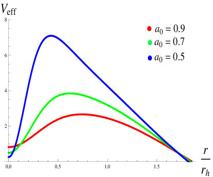
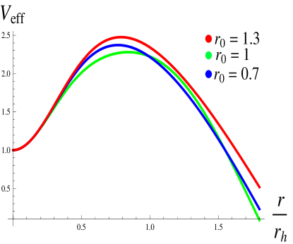
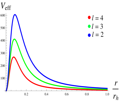
It is noted that the effective potential turns out to be zero at event horizons due to the vanishing of metric coefficient $G(r,\theta)$. For graphical analysis, we plot the effective potential versus $\frac{r}{r_{h}}$ to examine the impact of different parameters on gravitational barrier as shown in Figures 1-2. Firstly, we set the parameters $r_{0}=1=m$, $l=2$, $w=0.1$ and sketch the graphs for different choices of the rotation parameter. It is found that the height of potential barrier decreases with the increase in $a_{0}$ which causes an enhancement in the emission of scalar fields (left plot of Figure 1). As a result, the greybody factor increases significantly corresponding to larger values of rotation parameter. In the right plot of Figure 1, we display the effect of length parameter on the profile of effective potential. We observe that the gravitational potential is positive, finite and has a direct relation with $r_{0}$, i.e., increase in the values of $r_{0}$ leads to increase in the height of barrier which subsequently decreases the emission of scalar particles. The dependence of angular momentum numbers is also demonstrated in Figure 2 which shows that higher spikes of the effective potential are attained for larger values of $l$ and $m$ which ultimately minimize the emission process and greybody factor.

3 Greybody factor

In this section, we obtain an analytical solution of the greybody factor in low energy regime by using an approximation technique. We solve Eq.(5) for two asymptotic regions separately, i.e., close to BH horizon and far-away from it. These two solutions will be extended and matched smoothly in an intermediate region to get an analytical expression for the whole radial regime.

3.1 Analytical solution

For the near horizon regime $r\sim r_{h}$, we apply the transformation

$$r\rightarrow h=\frac{\Pi(r)}{r^{2}+a_{0}^{2}},$$ (14)

such that

$$\frac{dh}{dr}=\frac{(1-h)D(r_{h})}{r_{h}(r_{h}^{2}+a_{0}^{2})(r_{h}^{2}+r_{0}^{2})},$$ (15)

where

$$D(r_{h})=r_{h}^{4}-a_{0}^{2}r_{h}^{2}-2r_{0}^{2}r_{h}^{2}-4r_{0}^{2}a_{0}^{2}.$$ (16)

Using the above expressions in the radial equation of motion, we obtain

$\displaystyle h(1-h)\frac{d^{2}R_{wlm}}{dh^{2}}+(1-C_{*}h)\frac{dR_{wlm}}{dh}+[\frac{\chi^{*}}{D^{2}(r_{h})(1-h)h}-\frac{\lambda_{h}^{*}}{D^{2}(r_{h})(1-h)}]=0,$ (17)

where

$\displaystyle C_{*}$ $\displaystyle=$ $\displaystyle-\frac{(r_{h}^{2}+4r_{0}^{2})(r_{h}^{2}+a_{0}^{2})}{D(r_{h})},$ (18)
$\displaystyle\chi^{*}$ $\displaystyle=$ $\displaystyle r_{h}^{2}(r_{h}^{2}+r_{0}^{2})^{2}[w^{2}(r^{2}+a_{0}^{2})^{2}-a_{0}^{2}m^{2}-4a_{0}rM(r)],$ (19)

and

$\displaystyle\lambda_{h}^{*}$ $\displaystyle=$ $\displaystyle r_{h}^{2}(r_{h}^{2}+a_{0}^{2})(r_{h}^{2}+r_{0}^{2})^{2}[l(l+1)-\frac{2m^{2}-2l(l+1)+1}{(2l-1)(2l+3)}(a_{0}w)^{2}].$ (20)

In order to get a hypergeometric equation, we use the field redefinition

$$R_{wlm}(h)=h^{\mu_{1}}(1-h)^{\nu_{1}}\tilde{F}(h),$$ (21)

which reduces Eq.(17) to

$\displaystyle h(1-h)\frac{d^{2}\tilde{F}}{dh^{2}}+[1+2\mu_{1}-(2\mu_{1}+2\nu_{1}+C_{*})h]\frac{d\tilde{F}}{dh}+(\frac{\mu_{1}^{2}}{h}-\mu_{1}^{2}$
$\displaystyle+\mu_{1}-2\mu_{1}\nu_{1}-\nu_{1}^{2}+\frac{\nu_{1}^{2}}{1-h}-\frac{2\nu_{1}}{1-h}+\nu_{1}-\mu_{1}C_{*}+\frac{\nu_{1}C_{*}}{1-h}$
$\displaystyle-\nu_{1}C_{*}+\frac{\chi^{*}}{D^{2}h}+\frac{\chi^{*}}{D^{2}(1-h)}-\frac{\lambda_{h}^{*}}{D^{2}(1-h)})\tilde{F}=0.$ (22)

Here

$\displaystyle\tilde{a}=\mu_{1}+\nu_{1}+C_{*}-1,\quad\tilde{b}=\mu_{1}+\nu_{1},\quad\tilde{c}=1+2\mu_{1}.$ (23)

The power coefficients $\mu_{1}$ and $\nu_{1}$ can be calculated by second order algebraic equations (following the condition that coefficient of $\tilde{F}(h)$ must be $-\tilde{a}\tilde{b}$), namely,

$\displaystyle\mu_{1}^{2}+\frac{\chi^{*}}{D^{2}}$ $\displaystyle=$ $\displaystyle 0,$ (24)
$\displaystyle\nu_{1}^{2}+\nu_{1}(C_{*}-2)+\frac{\chi^{*}}{D^{2}}-\frac{\lambda_{h}^{*}}{D^{2}}$ $\displaystyle=$ $\displaystyle 0.$ (25)

The radial equation combined with Eq.(23) and constraints (24, 25) leads to

$$h(1-h)\frac{d^{2}\tilde{F}}{dh^{2}}+[\tilde{c}-(1+\tilde{a}+\tilde{b})h]\frac{d\tilde{F}}{dh}-\tilde{a}\tilde{b}\tilde{F}(h)=0.$$ (26)

Thus, the general solution of Eq.(22) in terms of hypergeometric function can be expressed as

$\displaystyle(R_{wlm})_{NH}(h)$ $\displaystyle=$ $\displaystyle A_{1}h^{\mu_{1}}(1-h)^{\nu_{1}}\tilde{F}(\tilde{a},\tilde{b},\tilde{c};h)$ (27)
$\displaystyle+$ $\displaystyle A_{2}h^{-\mu_{1}}(1-h)^{\nu_{1}}\tilde{F}(\tilde{a}-\tilde{c}+1,\tilde{b}-\tilde{c}+1,2-\tilde{c};h),$

where $A_{1}$ and $A_{2}$ are arbitrary constants with

$\displaystyle\mu_{1}^{\pm}$ $\displaystyle=$ $\displaystyle\pm\iota\frac{\chi^{*}}{D(r_{h})},$ (28)
$\displaystyle\nu_{1}^{\pm}$ $\displaystyle=$ $\displaystyle\frac{1}{2}[(2-C_{*})\pm\sqrt{(2-C_{*})^{2}-4(\frac{\chi^{*}}{D^{2}}-\frac{\lambda_{h}^{*}}{D^{2}})}].$ (29)

Applying the boundary constraint that no outgoing mode exists near the horizon of BH, we can take either $A_{1}=0$ or $A_{2}=0$ depending upon the signature of $\mu_{1}$. As these two constants become equivalent for both choices of $\mu_{1}$, so we opt $\mu_{1}=\mu_{1}^{-}$ and choose $A_{2}=0$. Similarly, the sign of $\nu_{1}$ can be decided by using the convergence property of hypergeometric function which is satisfied for $\nu_{1}=\nu_{1}^{-}$. Hence the final expression of near horizon solution is given as

$$(R_{wlm})_{NH}(h)=A_{1}h^{\mu_{1}}(1-h)^{\nu_{1}}\tilde{F}(\tilde{a},\tilde{b},\tilde{c};h).$$ (30)

Our next goal is to evaluate the solution of radial equation in the far-field regime. Using the assumption $r>>r_{h}$ and keeping the leading factor in the expansion of $\frac{1}{r}$, Eq.(5) takes the form

$$\frac{d^{2}\tilde{R}_{wlm}}{dr^{2}}+\frac{1}{r}\frac{d\tilde{R}_{wlm}}{dr}+\{w^{2}-\frac{1}{r^{2}}\frac{[l(l+1)+2(a_{0}w)^{2}(l(l+1)-1)]}{(2l-1)(2l+3)}+\frac{1}{4}\}\tilde{R}_{wlm}=0,$$ (31)

which is known as Bessel equation with $R_{wlm}(r)=\frac{1}{\sqrt{r}}\tilde{R}_{wlm}$. Thus, the solution in the far-field region is given as

$$(R_{wlm})_{FF}=\frac{\tilde{B}_{1}}{\sqrt{r}}J_{v}(wr)+\frac{\tilde{B}_{2}}{\sqrt{r}}Y_{v}(wr),$$ (32)

where $B_{1,2}$ are integration constants, $J_{v}(wr)$ and $Y_{v}(wr)$ are the Bessel functions with $v=\sqrt{l(l+1)+2(a_{0}w)^{2}\frac{(l(l+1)-1)}{(2l-1)(2l+3)}+\frac{1}{4}}$.

4 Matching to an Intermediate Regime

In order to obtain an analytical solution which remains valid for complete range of $r$, we have to match the obtained solutions smoothly in the intermediate region. For this purpose, we first stretch the near horizon solution by exchanging the argument of hypergeometric function from $h$ to $1-h$ as

$\displaystyle(R_{wlm})_{NH}(h)$ $\displaystyle=$ $\displaystyle A_{1}h^{\mu_{1}}(1-h)^{\nu_{1}}\{\frac{\Gamma(\tilde{c})\Gamma(\tilde{c}-\tilde{a}-\tilde{b})}{\Gamma(\tilde{c}-\tilde{a})\Gamma(\tilde{c}-\tilde{b})}\tilde{F}(\tilde{a},\tilde{b},\tilde{c};1-h)$ (33)
$\displaystyle+$ $\displaystyle(1-h)^{\tilde{c}-\tilde{a}-\tilde{b}}\frac{\Gamma(\tilde{c})\Gamma(\tilde{a}+\tilde{b}-\tilde{c})}{\Gamma(\tilde{a})\Gamma(\tilde{b})}$
$\displaystyle\times$ $\displaystyle\tilde{F}(\tilde{c}-\tilde{a},-\tilde{b}+\tilde{c},\tilde{c}-\tilde{b}-\tilde{a}+1;1-h)\}.$

Using horizon equation, the function $h(r)$ can be expressed as

$$h(r)=1-\frac{r}{r_{h}}\left[\frac{1+a_{*}^{2}}{(\frac{r}{r_{h}})^{2}+a_{*}^{2}}\right],$$ (34)

with $a_{*}=\frac{a_{0}}{r_{h}}$. When $r>>r_{h}$, the term $(\frac{r}{r_{h}})^{2}$, appearing in the second factor, becomes dominant which leads the whole expression towards unity. In the limiting value $h\rightarrow 1$, we have

$$(1-h)^{\nu_{1}}\simeq(\frac{r_{h}}{r})^{\nu_{1}},$$ (35)

and

$$(1-h)^{\nu_{1}+\tilde{c}-\tilde{a}-\tilde{b}}\simeq(\frac{r_{h}}{r})^{-\nu_{1}+2-C_{*}}.$$ (36)

Thus, the near horizon solution in an intermediate region becomes

$$(R_{wlm})_{NH}(r)=A^{*}_{1}r^{-\nu_{1}}+A^{*}_{2}{r}^{\nu_{1}-2+C_{*}},$$ (37)

with

$\displaystyle A^{*}_{1}$ $\displaystyle=$ $\displaystyle A_{1}[(1+a_{*}^{2})r_{h}]^{\nu_{1}}\frac{\Gamma(\tilde{c})\Gamma(\tilde{c}-\tilde{a}-\tilde{b})}{\Gamma(\tilde{c}-\tilde{a})\Gamma(\tilde{c}-\tilde{b})},$ (38)
$\displaystyle A^{*}_{2}$ $\displaystyle=$ $\displaystyle A_{1}[(1+a_{*}^{2})r_{h}]^{(-\nu_{1}-C_{*}+2)}\frac{\Gamma(\tilde{c})\Gamma(\tilde{a}+\tilde{b}-\tilde{c})}{\Gamma(\tilde{a})\Gamma(\tilde{b})}.$ (39)

Setting the limit $wr\rightarrow 0$ in Eq.(32) to shift the far-field solution towards the smaller values of $r$, we obtain

$\displaystyle(R_{wlm})_{FF}$ $\displaystyle\simeq$ $\displaystyle\frac{B_{1}(\frac{wr}{2})^{\sqrt{\lambda_{l}^{m}+\frac{1}{4}-w^{2}a_{0}^{2}}}}{\sqrt{r}\Gamma(\sqrt{\lambda_{l}^{m}+\frac{1}{4}-w^{2}a_{0}^{2}}+1)}$ (40)
$\displaystyle-$ $\displaystyle\frac{B_{2}\Gamma(\sqrt{\lambda_{l}^{m}+\frac{1}{4}-w^{2}a_{0}^{2}})(\frac{wr}{2})^{-\sqrt{\lambda_{l}^{m}+\frac{1}{4}-w^{2}a_{0}^{2}}}}{\sqrt{r}\pi}.$

We observe that power coefficients of the radial component in both solutions are different from each other which restrain the exact matching. To resolve this problem, the power-law expressions are expanded in the limit $(\frac{a_{0}}{r_{h}})^{2}<<1$ and $(wr_{h})^{2}<<1$. These approximations restrict the accuracy of our solutions in the low rotation and low energy region. In this expansion, we also ignore the second order term $(a_{0}w)^{2}$ to achieve the smooth matching. Employing these restrictions, Eq.(37) takes the form

$\displaystyle-\nu_{1}$ $\displaystyle=$ $\displaystyle l+O(w_{*}^{2},a_{*}^{2},w_{*}a_{*}),$ (41)
$\displaystyle\nu_{1}-2+C_{*}$ $\displaystyle=$ $\displaystyle-(l+1)+O(w_{*}^{2},a_{*}^{2},w_{*}a_{*}).$ (42)

Similarly, the power coefficient in Eq.(40) reduces to

$$\sqrt{\lambda_{l}^{m}+\frac{1}{4}-w^{2}a_{0}^{2}}=(l+\frac{1}{2})+O(w_{*}^{2}a_{*}^{2}).$$ (43)

It is worth mentioning here that all aforementioned approximations are not used in the argument of gamma function to increase the efficiency of our results. One can easily check that both asymptotic solutions have the same power coefficients, i.e., $r^{l}$ and $r^{-(l+1)}$. Therefore, we can determine the integration constants by comparing the corresponding coefficients of Eqs.(37) and (40). Thus, the matching of these two solutions leads to

$\displaystyle\tilde{B}$ $\displaystyle=$ $\displaystyle\frac{\tilde{B}_{1}}{\tilde{B}_{2}}=\frac{1}{\pi}(\frac{2}{w(1+a_{*}^{2})r_{h}})^{2l+1}\sqrt{\lambda_{l}^{m}+\frac{1}{4}-w^{2}a_{0}^{2}}$ (44)
$\displaystyle\times$ $\displaystyle\frac{\Gamma^{2}(\sqrt{\lambda_{l}^{m}+\frac{1}{4}-w^{2}a_{0}^{2}})\Gamma(\tilde{a})\Gamma(\tilde{b})\Gamma(\tilde{c}-\tilde{a}-\tilde{b})}{\Gamma(\tilde{c}-\tilde{a})\Gamma(\tilde{c}-\tilde{b})\Gamma(\tilde{a}+\tilde{b}-\tilde{c})},$

which ensures an analytical smooth solution of the radial equation for all choices of $r$, valid in low angular momentum and low energy region.

Finally, to compute the greybody factor, we stretch Eq.(32) to $r\rightarrow\infty$ which leads to

$\displaystyle(R_{wlm})_{FF}(r)$ $\displaystyle\simeq$ $\displaystyle\frac{1}{\sqrt{2\pi w}}\left[\frac{\tilde{B}_{1}+\iota\tilde{B}_{2}}{r}\exp{-\iota(wr-\frac{\pi}{2}v-\frac{\pi}{4})}\right.$ (45)
$\displaystyle+$ $\displaystyle\left.\frac{\tilde{B}_{1}-\iota\tilde{B}_{2}}{r}\exp{\iota(wr-\frac{\pi}{2}v-\frac{\pi}{4})}\right],$
$\displaystyle=$ $\displaystyle\tilde{A}_{in}^{(\infty)}\frac{\exp^{-\iota wr}}{r}+\tilde{A}_{out}^{(\infty)}\frac{\exp^{\iota wr}}{r}.$ (46)

The effects of rotation parameter become negligible at a large distance from BH. This reduces our massless scalar field solution to a spherical wave [34]-[36] allowing to calculate the greybody factor as

$\displaystyle|\tilde{\emph{A}}_{l,m}|^{2}$ $\displaystyle=$ $\displaystyle 1-\left|\frac{\tilde{A}_{out}^{(\infty)}}{\tilde{A}_{in}^{(\infty)}}\right|^{2}=1-\left|\frac{\tilde{B}_{1}-\iota\tilde{B}_{2}}{\tilde{B}_{1}+\iota\tilde{B}_{2}}\right|^{2},$ (47)
$\displaystyle=$ $\displaystyle 1-\left|\frac{\tilde{B}-\iota}{\tilde{B}+\iota}\right|^{2}=\frac{2\iota(\tilde{B}^{*}-\tilde{B})}{\tilde{B}\tilde{B}^{*}+\iota(\tilde{B}^{*}-\tilde{B})+1}.$ (48)

The above expression, together with Eq.(44), is the main result for the greybody factor specifying the emission of massless scalar field from a rotating regular BH.

Since any traveling wave passing the far-field horizon will face the potential barrier as a hindrance, therefore some of its part will be transmitted towards the horizon of BH and some is reflected back to the far-field regime. Basically, it is the relative relation between the effective potential and frequency which decides either to reflect back the wave or move forward. When the frequency of the wave is larger than the effective barrier, it can cross the barrier and will not be reflected back. In the reverse case, when the height of potential is larger as compared to the frequency, most of the part will be reflected towards the far-field region and some of its portion may cross the barrier through the tunneling effect. In this scenario, the greybody factor shows a negative trend.

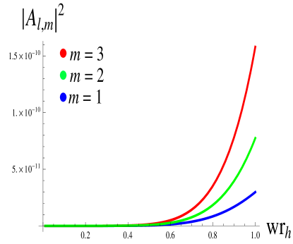
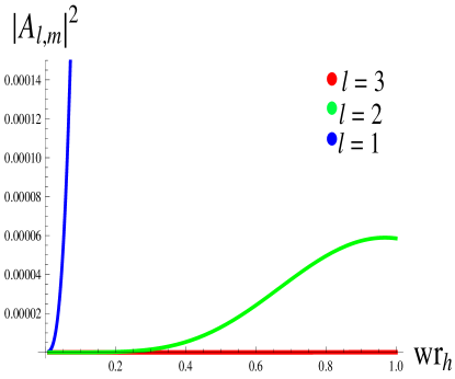
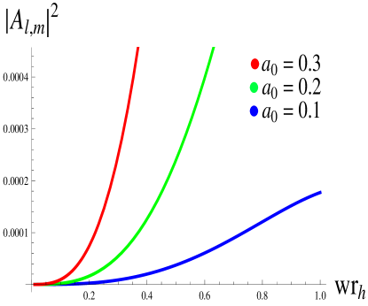
To study the characteristics of greybody factor in detail, we sketch our main expressions, given by Eqs.(44) and (48), for scalar particle $(l,m)$ and spacetime $(a_{0},r_{0})$ variables. It is noted that the greybody factor remains positive throughout the considered domain of dimensionless parameter $wr_{h}$. In Figure 3, we fix the spacetime variables and plot the graphs for discrete choices of angular momentum numbers. It is found that the increase in the values of $m$ leads to larger ranges of the greybody factor (left plot) whereas the reverse effects are observed for orbital angular momentum (right plot). One can easily observe that the partial wave with $l=1$ dominates in the low energy region while all higher modes strongly minimize the absorption probability. The impact of $r_{0}$ and $a_{0}$ on the greybody factor are shown in Figure 4. We note that increase in the values of rotation as well as length parameter yields the higher values of absorption probability.

Refer to caption
Refer to caption
Figure 3: Greybody factor for massless scalar field corresponding to $a_{0}=0.1$, $l=3$ (left plot) and $m=1$, $a_{0}=0.5$ (right plot) with $r_{0}=0.5$.
Refer to caption
Refer to caption
Figure 4: Greybody factor for massless scalar field corresponding to $r_{0}=0.5$ (left plot) and $a_{0}=0.5$ (right plot) with $m=l=1$.

The particle flux, i.e., the total amount of massless scalar particles discharged per unit time and frequency from a BH is given by

$\displaystyle\frac{d^{2}\tilde{N}}{dtdw}=\frac{1}{2\pi}\sum_{l,m}\frac{1}{e^{\frac{k}{T_{H}}-1}}|\tilde{\emph{A}}_{l,m}|^{2},\quad k=w-\frac{ma_{0}}{r_{h}^{2}+a_{0}^{2}},$ (49)

and Hawking temperature is defined as

$\displaystyle T_{H}$ $\displaystyle=$ $\displaystyle\frac{(1-a_{*}^{2})}{4\pi(1+a_{*}^{2})r_{h}}.$ (50)

Moreover, the energy emission rate is found to be

$\displaystyle\frac{d^{2}\tilde{E}}{dtdw}=\frac{1}{2\pi}\sum_{l,m}\frac{w}{e^{\frac{k}{T_{H}}-1}}|\tilde{\emph{A}}_{l,m}|^{2},$ (51)

which, through Eq.(48), gives rise to

$\displaystyle\frac{d^{2}\tilde{E}}{dtdw}=\frac{1}{2\pi}\sum_{l,m}\frac{w}{e^{\frac{k}{T_{H}}-1}}\frac{2\iota(\tilde{B}^{*}-\tilde{B})}{\tilde{B}\tilde{B}^{*}+\iota(\tilde{B}^{*}-\tilde{B})+1}.$ (52)

Similarly, we can write differential equation for the angular momentum emission rate. As the greybody factor depends upon both particle as well as spacetime properties, therefore it changes the various emission rates, accordingly. The absorption cross-section for each partial wave has the form

$\displaystyle\sigma=\frac{\pi}{w^{2}}\sum_{l,m}|\tilde{\emph{A}}_{l,m}|^{2}.$ (53)

Using Eq.(48), it follows that

$\displaystyle\sigma=\frac{\pi}{w^{2}}\sum_{l,m}\frac{2\iota(\tilde{B}^{*}-\tilde{B})}{\tilde{B}\tilde{B}^{*}+\iota(\tilde{B}^{*}-\tilde{B})+1}.$ (54)

5 Conclusions

This work is devoted to formulating an analytical form of the greybody factor for rotating Bardeen regular BH. For this purpose, we have studied the profile of gravitational barrier which is the basic reason to generate the absorption probability. We have evaluated two asymptotic solutions from the radial equation of motion at different horizons which are valid in low rotation and low energy region. To obtain a general expression of the greybody factor, we have stretched these solutions and matched them smoothly to an intermediate regime. Finally, we have calculated the emission rates and absorption cross-section for the massless scalar field. The results are summarized as follows.

We have examined the behavior of angular momentum numbers $(l,m)$ and topological parameters $(a_{0},r_{0})$ of spacetime on the effective potential as well as greybody factor. It is found that the height of gravitational barrier for the massless scalar field decreases with increasing $a_{0}$ while the larger modes of length parameter correspond to higher values of the potential barrier which ultimately reduce the emission rate of Hawking radiation (Figures 1-2). From the graphical display of absorption probability against the parameter $wr_{h}$, we observe that it attains positive values in the considered domain and an increase in the parameter $m$ causes an enhancement in the greybody factor (Figure 3). For the orbital angular momentum, partial wave with smaller value $(l=1)$ dominates in the low approximation limit while all higher values significantly reduce the greybody factor as in the case of rotating BH [21]. Moreover, higher modes of rotation and length parameter yield higher values of the absorption probability (Figure 4). We conclude that the rotation parameter effectively increases the scalar emission rate for rotating Bardeen BH which is consistent with the literature [21].

The greybody factor of a BH can be used to measure its evaporation rate because it is just the probability of a wave to transmit through the potential barrier to reach infinity. Based upon our analysis, it can be seen that regular as well as rotating BH evaporates more quickly as compared to other BH spacetimes. These BHs radiate more thermal flux of quantum particles and hence can be expected to lose their mass, comparatively, in a short span. Hence the rotating Bardeen BH being the larger emitter of scalar field particles would shrink and dissipate faster.

According to the no-hair theorem, all astrophysical BH candidates have correspondence with Kerr BHs, but the existing nature of these objects still need to be verified [37]. The impact of the parameter $r_{0}$ on the effective potential, greybody factor and absorption cross-section presents a good theoretical opportunity to individualize the rotating Bardeen BH from the Kerr BH and to test whether astrophysical BH candidates are the actual BHs as predicted by general relativity.

Acknowledgement

One of us (QM) would like to thank the Higher Education Commission, Islamabad, Pakistan for its financial support through the Indigenous Ph.D. Fellowship, Phase-II, Batch-III.

References

  • [1] Bardeen, J.M.: Proceedings of GR5 (Tiflis, USSR, 1968)174.
  • [2] Cataldo, M. and Garc$\acute{i}$a, A.: Phys. Rev. D 61(2000)084003.
  • [3] Bronnikov, K.A.: Phys. Rev. D 63(2001)044005.
  • [4] Dymnikova, I.: Class. Quantum Grav. 21(2004)4417.
  • [5] Hayward, S.: Phys. Rev. Lett. 96(2006)031103.
  • [6] Berej, W. et al.: Gen. Relativ. Gravit. 38(2006)885.
  • [7] Ghosh, S.G. and Maharaj, S.D.: Eur. Phys. J. C 75(2015)7.
  • [8] Newman, E.T. and Janis, A.I.: J. Math. Phys. 6(1965)915.
  • [9] Ay$\acute{o}$n-Beato, E. and Garc$\acute{i}$a, A.: Phys. Lett. B 493(2000)149.
  • [10] Drake, S.P. and Szekeres, P.: Gen. Relativ. Gravit. 32(2000)445.
  • [11] Bambi, C. and Modesto, L.: Phys. Lett. B 721(2013)329.
  • [12] Hawking, S.W.: Commun. Math. Phys. 43(1975)199.
  • [13] Parikh, M.K. and Wilczek, F.: Phys. Rev. Lett. 85(2000)5042.
  • [14] Kerner, R. and Mann, R.B.: Class. Quantum Grav. 25(2008)095014.
  • [15] Ejaz, A. et al.: Phys. Lett. B 726(2013)827.
  • [16] Ford, L.H.: Phys. Rev. D 12(1975)2963.
  • [17] Gubserv, S.S. and Klebanov, I.R.: Phys. Rev. Lett. 77(1996)4491.
  • [18] Maldacena, J.M. and Strominger, A.: Phys. Rev. D 55(1997)861.
  • [19] Klebanov, I.R. and Mathur, S.D.: Nucl. Phys. B 500(1997)115.
  • [20] Kim, W.T. and Oh, J.J.: Phys. Lett. B 461(1999)189.
  • [21] Creek, S. et al.: Phys. Lett. B 656(2007)102.
  • [22] Creek, S. et al.: Phys. Rev. D 75(2007)084043.
  • [23] Boonserm, P. et al.: J. Math. Phys. 55(2014)112502.
  • [24] Jorge, R., de Oliveira, E.S. and Rocha, J.V.: Class. Quantum Grav. 32(2015)065008.
  • [25] Toshmatov, B. et al.: Phys. Rev. D 91(2015)083008.
  • [26] Ahmad, J. and Saifullah, K.: Eur. Phys. J. C 77(2017)885.
  • [27] Dey, S. and Chakrabarti, S.: Eur. Phys. J. C 79(2019)504.
  • [28] Hyun, Y.H., Kimb, Y. and Park, S.C.: J. High Energy Phys. 2019(2019)41.
  • [29] Azreg-A nou, M.: Eur. Phys. J. C 74(2014)2865.
  • [30] Flammer, C.: Spheroidal Wave Functions (Stanford University Press, 1957).
  • [31] Goldberg, J.N. et al.: J. Math. Phys. 8(1967)2155.
  • [32] Berti, E., Cardoso, V. and Casals, M.: Phys. Rev. D 73(2006)024013.
  • [33] Berti, E., Cardoso, V. and Casals, M.: Phys. Rev. D 73(2006)109902.
  • [34] Kanti, P. and March-Russell, J.: Phys. Rev. D 66(2002)024023.
  • [35] Kanti, P. and March-Russell, J.: Phys. Rev. D 67(2003)104019.
  • [36] Harris, C.M. and Kanti, P.: Phys. Lett. B 633(2006)106.
  • [37] Bambi, C.: Phys. Lett. B 730(2014)59.