Receptive-Field-Regularized CNN Variants for
Acoustic Scene Classification

Abstract

Acoustic scene classification and related tasks have been dominated by Convolutional Neural Networks (CNNs) [2, 3, 4, 5, 6, 7, 8, 9, 10]. Top-performing CNNs use mainly audio spectograms as input and borrow their architectural design primarily from computer vision. A recent study [1] has shown that restricting the receptive field (RF) of CNNs in appropriate ways is crucial for their performance, robustness and generalization in audio tasks. One side effect of restricting the RF of CNNs is that more frequency information is lost. In this paper, we perform a systematic investigation of different RF configuration for various CNN architectures on the DCASE 2019 Task 1.A dataset. Second, we introduce Frequency Aware CNNs to compensate for the lack of frequency information caused by the restricted RF, and experimentally determine if and in what RF ranges they yield additional improvement. The result of these investigations are several well-performing submissions to different tasks in the DCASE 2019 Challenge.

Index Terms—  Acoustic Scene Classification, Frequency-Aware CNNs, Receptive Field Regularization

1 Introduction

Convolutional Neural Networks (CNNs) have shown great promise as end-to-end classifiers in many tasks such as image classification [11, 12] and acoustic scene classification [5, 13]. Although every year new architectures are proposed that achieve better image recognition performance, we showed in a recent study [1] that these performance gains do not seem to translate to the audio domain. As a solution, we proposed regularizing the receptive field (RF) of such CNN architectures in specific ways. The method was applied to several state-of-the-art image recognition architectures, and the resulting models were shown to then achieve state-of-the-art performance in audio classification tasks [1].

Although CNNs can learn their own features and build internal representations from data, the details of how they actually function is crucial to their success in a specific task. In the image recognition domain, a recent study [14] shed light on the decision making procedure of CNNs and showed that using occurrences of small local image features without taking into account their spatial ordering, CNNs can still achieve state-of-the-art results. However, while spatial ordering and local neighboring relations might not be crucial for object recognition in images, this is not the case in audio representations such as spectrograms. A local pattern in lower frequencies does not represent the same acoustic event as the same pattern appearing in higher frequencies. Since CNNs with limited receptive fields are only capable of capturing local features and unlike models such as capsule networks [15], they are unable to find spatial relations between these local patterns. As convolution is equivariant, each filter is applied to the input to generate an output activation, but the output of the network does not know where exactly each filter is. This means that if a specific pattern appears in lower frequencies, and a very similar pattern appears in higher frequencies, later convolutional layers cannot distinguish between the two, and this can result in vulnerabilities in such cases.

In [16], Liu et al. analyzed a generic inability of CNNs to map a pixel in a 2D space, to its exact cartesian coordinate. They address this problem by adding an additional channel to the convolutional layers that contains only the pixel coordinates. Inspired by this solution, we propose a new convolutional layer for audio processing – the Frequency-aware Convolutional Layer – to cope with the aforementioned problems in CNNs. We use an additional channel in the convolutional layer that only contains the frequency information which connects each filter to the frequency bin it is applied to.

In this paper, we extend our previous work [1] by modifying the receptive field (RF) of various new architectures such as Resnet [11], PreAct ResNet [17, 18], Shake-shake [19, 18], Densenet [12], and our new frequency-aware FAResNet according to the guidelines provided in [1], aiming at pushing the performance of these models on acoustic scene classification tasks. Systematic experiments permit us to determine optimal RF ranges for various architectures on the DCASE 2019 datasets. We show that configuring CNNs to have a receptive field in these ranges has a significant impact on their performance. Based on these insights, we configured network classifiers that achieved a number of top results in several DCASE 2019 challenge tasks [13], as will be briefly reported in Section 4.3.

2 Regularizing CNN Architectures and Introducing Frequency Awareness

Table 1: Modified ResNet architectures

RB Number	RB Config
	Input $5\times 5$ stride=$2$
1	$3\times 3$, $1\times 1$, P
2	$x_{1}\times x_{1}$, $x_{2}\times x_{2}$, P
3	$x_{3}\times x_{3}$, $x_{4}\times x_{4}$
4	$x_{5}\times x_{5}$, $x_{6}\times x_{6}$, P
5	$x_{7}\times x_{7}$, $x_{8}\times x_{8}$
6	$x_{9}\times x_{9}$, $x_{10}\times x_{10}$
7	$x_{11}\times x_{11}$, $x_{12}\times x_{12}$
8	$x_{13}\times x_{13}$, $x_{14}\times x_{14}$
9	$x_{15}\times x_{15}$, $x_{16}\times x_{16}$
10	$x_{17}\times x_{17}$, $x_{18}\times x_{18}$
11	$x_{19}\times x_{19}$, $x_{20}\times x_{20}$
12	$x_{21}\times x_{21}$, $x_{22}\times x_{22}$
RB: Residual Block, P: $2\times 2$ max pooling after the block.
$x_{k}\in\{1,3\}$: hyper parameter we use to control the RF
of the network. Number of channelds per RB:
128 for RBs 1-4; 256 for RBs 5-8; 512 for RBs 9-12.

Table 2: Mapping $\rho$ values to the maximum RF of ResNet variants (networks configured as in Table 1). $\rho$ controls the maximum RF by setting the $x_{k}$ as explained in Eq. (1).

$\rho$ value	Max RF	$\rho$ value	Max RF
0	$23\times 23$	1	$31\times 31$
2	$39\times 39$	3	$55\times 55$
4	$71\times 71$	5	$87\times 87$
6	$103\times 103$	7	$135\times 135$
8	$167\times 167$	9	$199\times 199$
10	$231\times 231$	11	$263\times 263$
12	$295\times 295$	13	$327\times 327$
14	$359\times 359$	15	$391\times 391$
16	$423\times 423$	17	$455\times 455$
18	$487\times 487$	19	$519\times 519$
20	$551\times 551$	21	$583\times 583$

As shown in our previous work [1], the size of the receptive field (RF) is crucial when applying CNNs to audio recognition tasks. Following the guidelines in [1], we adapted various ResNet and DenseNet variants. Using the provided development set for Task 1.A [20], we performed a grid search on the RF of the various ResNet architectures and show the performance of different CNNs under different RF setups. The goal of this investigation, reported in Section 2.1.1, is to introduce a method to systematically push the performance of a single CNN architecture for acoustic scene classification. We base on this method our submissions [13] to the DCASE 2019 challenge[21], especially our top performing single architecture submission for Task 1.A (cp_resnet).

Furthermore, in Section 2.2 we introduce Frequency-aware CNNs to address the possible shortcomings of models with a smaller receptive field. Systematic experiments will then show whether, or in what cases, this actually helps improve the results.

2.1 Adapting the Receptive Field of CNNs

2.1.1 ResNet

ResNet [11] and its variants (such as preact-ResNet [17]) achieve state-of-the-art results in image recognition. As we show in our recent study [1], such architectures can be adapted to audio tasks using RF regularization. We adapt the RF of the ResNet in a similar fashion to  [1] as explained below. The resulting network architectures are detailed in Table 1. We use the hyper-parameters $x_{k}\in\{1,3\}$, corresponding to filter sizes at different CNN levels (see Fig. 1), to control the RF of the network. In order to simplify the process of adjusting the RF of the network, we introduce a new hyper-parameter $\rho$. We use $\rho$ to control $x_{k}$ as explained in  (1).

$$x_{k}=\begin{cases}3&\quad\text{if }k\leq\rho\\ 1&\quad\text{if }k>\rho\\ \end{cases}$$ (1)

For example, setting $\rho=5$ will result in a ResNet configured as in Table 1 with $x_{k}=3\text{ for }k\in[1,5]$ and $x_{k}=1\text{ otherwise}$. The resulting ResNet has a RF of $87\times 87$. Table 2 maps $\rho$ values to the maximum RF of the resulting network.

Networks with larger receptive fields degrade in performance as shown in [1]. For this reason, we present the results of $\rho$ values in the range $\rho\in[1,12]$

2.1.2 PreAct ResNet

PreAct ResNet is a ResNet variant where residual branches are summed up before applying the non-linearity [17]. We specifically use PreActBN as explained in [18], since it improves the performance of vanilla PreAct ResNet with and without Shake-Shake regularization for speech emotion recognition.

We control the RF of PreAct ResNets in the same manner as ResNets (Section 2.1.1). Table 1 and Equation 1 explain the configurations of our tested networks.

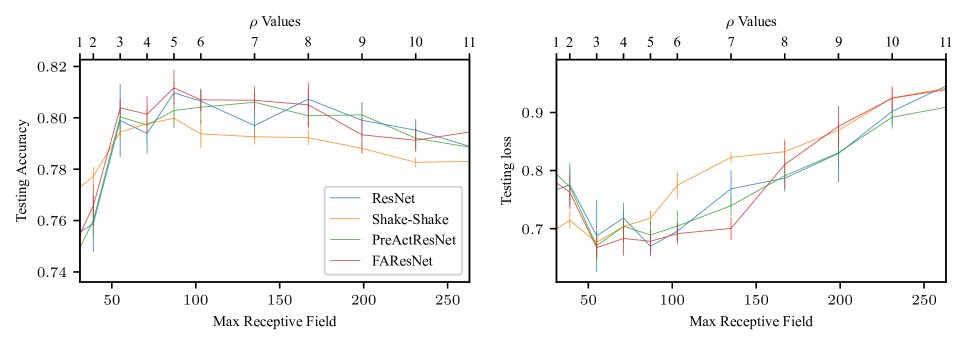
Figure 1: Testing Loss/Accuracy of the provided development split of Task 1 a dataset, for ResNet variants with different receptive fields over the input without mix-up.

2.1.3 Shake-Shake ResNet

The Shake-Shake architecture [19] is a variant of ResNet that is proposed for improved stability and robustness. Each residual block has 3 branches; an identity map of the input and 2 convolutional branches, which are summed with random coefficients (in both the forward and backward pass) [19]. This regularization technique has shown empirically to improve the performance of CNNs on many tasks. We also specifically use Shake-Shake regularized PreActBN from [18]. In Shake-Shake regularized ResNets, each residual block only has a new branch that is added to the sum. Therefore, the resulting maximum RF of the network is not changed. In result, we use the same techniques to control the RF (Section 2.1.1). Table 1 shows the configuration of both branches of the residual blocks.

Although, Shake-Shake ResNet is not performing well in the classic acoustic scene classification problem (as shown in Section 4), it excels in the case of domain mismatch (Task 1.B [20, 21]) and noisy datasets (Task 2 [22]) [13].

2.1.4 DenseNet

We adapted DenseNet [12] in a similar fashion to DN1 in  [1]. We report on two DenseNet configurations with maximum RF of $87\times 87$ and $71\times 71$ pixels (Section 4).

2.2 Frequency-aware Convolution

In CNNs that have a large enough RF, deeper convolutional layers can infer the frequency information of their input feature maps. However, CNNs with large RF degrade in performance and fail to generalize in acoustic scene classification as shown in [1]. On the other hand, in high-performing fully convolutional CNNs, learned CNN filters are agnostic to the frequency range information of the feature maps. In other words, the spectrograms and feature maps can be rolled over both the time and frequency dimension with a minor impact on the network predictions. This is one side effect of limiting the receptive field of CNNs on spectograms. We propose a new convolutional layer, which we call Frequency-aware Convolution, to make filters aware and more specialized in certain frequencies by concatenating a new channel containing the frequency information of each spatial pixel to each feature map. This technique is similar to CoordConv [16], where the network input is padded with the pixels’ coordinates. In our case, we pad all feature maps with a real number indicating the frequency context of each pixel.

The CNN models that incorporate our frequency-aware layer will be called the Frequency-Aware Convolutional Neural Networks (FACNNs). Similarly, we call the frequency-aware ResNet FAResNet. We denote the value of the pixel with spatial index $(f,t)$ in the new channel as $V(f,t)$; it is calculated as

$$V(f,t)=f/F$$ (2)

where $F$ is the size of the frequency dimension of the feature map, $f$ is the pixel index in the frequency dimension, and $t$ is the pixel index in the time dimension. This new channel gives the convolutional filters a frequency context.

Since making CNNs frequency-aware (by adding the new channel) does not alter the maximum RF of the network, we control the maximum RF of FAResNets similar to ResNet (Section 2.1.1) by changing $\rho$.

3 Experimental Setup

Figure 2: Testing Loss/Accuracy of the provided development split of Task 1 a dataset, for ResNet variants with different receptive fields over the input with mix-up.

3.1 Data Preparation and Training

We extracted the input features using a Short Time Fourier Transform (STFT) with a window size of 2048 and 25% overlap. We perceptually weight the resulting spectrograms and apply a Mel-scaled filter bank in a similar fashion to Dorfer et al. [5]. This preprocessing results in 256 Mel frequency bins. The input is first down-sampled to 22.05 kHz. We process each input channel of the stereo audio input independently and provide the CNN with a two-channel-spectrogram input. The input frames are normalized using the training set mean and standard deviation.

We used Adam [23] with a specific scheduler. We start training with a learning rate of $1\times 10^{-4}$. From epoch 50 until 250, the learning rate decays linearly from $1\times 10^{-4}$ to $5\times 10^{-6}$. We train for another 100 epochs with the minimum learning rate $5\times 10^{-6}$ in a setup similar to [1].

3.2 Testing Setup

We use the provided development split of DCASE 2019 task 1A [20, 21]. We train our models on the provided training set and treat the provided test set as unseen set. In other words, we don’t select best models based on their performance on the test set. Instead, for each model, we report the average results of the last 25 training epochs of two runs on the test set.

3.3 Data Augmentation

Mix-Up: Mix-up [24] is an effective augmentation method that works by linearly combining two input samples and their targets. It was shown to have a great impact on the performance and the generalization of the models.
Spectogram Rolling: We roll the spectograms randomly over the time dimension.

4 Results

Table 3 shows the $\rho$ and Max RF configuration that achieves the top accuracy (mean/std over the last 25 epochs) for each architecture, with and without mix-up. It is also worth noting that the maximum RF is different from the effective RF as explained in  [1, 25]. We control the maximum RF using $\rho$, while the effective RF is dependent on the architecture, the initialization and the data [25]. This is one possible explanation for why different architectures may have a slightly shifted optimal maximum RF range (for example, PreAct in Table 3 and Figure 2). Likewise, using mix-up can alter the optimal maximum RF range for the networks.

4.1 Without Mix-up

Figure 1 shows the testing loss and accuracy for different architectures over a range of $\rho$ values and – consequently (see Eq. (1)) – maximum RF values. The plots summarize the results for the last 25 epochs of 2 runs. We notice that FAResNet excels mostly in smaller RF networks ($\rho<8$) where frequency context is more valuable. The figure also shows the best-performing maximum RF range for different architectures to correspond to $\rho$ values in the range $[3,8]$. In this range, FAResNet outperforms other ResNet variants.

4.2 With Mix-up

Figure 2 shows the testing loss and accuracy when we use mix-up data augmentation. We note that when using mix-up, ResNet outperforms the other variants. Further experiments and investigation are still needed to fully understand the effect of mix-up on these architectures. The figure shows that the best-performing maximum RF range for architectures corresponds to $\rho$ values in the range $[3,5]$ for ResNet and FAResNet, and $[4,6]$ for PreActResnet. Shake-Shake achieves its best performance for $\rho=4$. We see that performance degrades outside these maximum RF ranges for different architectures, in accordance with [1].

Table 3: Configurations with top accuracy per network architecture and its corresponding $\rho$ and max RF values with/without mix-up

Network	$\rho$	Max RF	M/U	Accuracy
ResNet	4	$71\times 71$	✓	$\textbf{82.85\%}\pm\textbf{.36}$
PreAct	5	$87\times 87$	✓	$82.62\%\pm.37$
Shake-Shake	4	$71\times 71$	✓	$80.47\%\pm.32$
FAResNet	4	$71\times 71$	✓	$82.66\%\pm.27$
DenseNet		$71\times 71$	✓	$81.53\%\pm.26$
ResNet	5	$87\times 87$	✗	$80.97\%\pm.46$
PreAct	7	$135\times 135$	✗	$80.6\%\pm.61$
Shake-Shake	5	$87\times 87$	✗	$79.98\%\pm.27$
FAResNet	5	$87\times 87$	✗	$\textbf{ 81.17 \% }\pm\textbf{.7}$
DenseNet		$87\times 87$	✗	$79.9\%\pm.3$
M/U: using Mix-Up

4.3 Performance at DCASE 2019

Our receptive field regularized networks achieved the second place [13] (team ranking) in Task 1.A of the DCASE 2019 challenge [21, 20]. We averaged ResNet, PreAct and FAResNet configured with $\rho=5$ to achieve $83.8\%$ accuracy on the evaluation set. Our ResNet configured with $\rho=5$ (our single architecture submission cp_resnet) achieved $82.8\%$ accuracy when trained on the whole development set; we averaged the prediction of the last training epochs [13]. When instead averaging the predictions of the same architecture trained on a 4-fold cross-validation of the development data, it achieves $83.7\%$ accuracy on the evaluation set. Furthermore, the submission achieved the highest accuracy on the unseen cities in the evaluation set ($78.1\%$).

The generality and robustness of the proposed RF regularization strategy is demonstrated by the fact that our highly-performing submissions to DCASE 2019 Tasks 1.B and 2 [13] are also based on these architectures.

5 Conclusion

In this paper, we have investigated different configurations of deep CNN architectures that correspond to different maximum receptive fields over audio spectograms. We showed that this helps to better design deep CNNs for acoustic classification tasks, and to adapt CNNs performing well in other domains (notably, image recognition) to acoustic scene classification. The good results achieved with this basic strategy in several DCASE 2019 tasks suggest that this is a very general and robust approach that may prove beneficial in various other audio processing tasks.

6 ACKNOWLEDGMENT

This work has been supported by the COMET-K2 Center of the Linz Center of Mechatronics (LCM) funded by the Austrian federal government and the Federal State of Upper Austria.

References

- [1] K. Koutini, H. Eghbal-zadeh, M. Dorfer, and G. Widmer, “The Receptive Field as a Regularizer in Deep Convolutional Neural Networks for Acoustic Scene Classification,” in Proceedings of the European Signal Processing Conference (EUSIPCO), A Coruña, Spain, 2019.
- [2] H. Eghbal-Zadeh, B. Lehner, M. Dorfer, and G. Widmer, “CP-JKU submissions for DCASE-2016: A hybrid approach using binaural i-vectors and deep convolutional neural networks,” in DCASE 2016-challenge on Detection and Classification of Acoustic Scenes and Events. DCASE2016 Challenge, 2016.
- [3] S. Hershey, S. Chaudhuri, D. P. W. Ellis, J. F. Gemmeke, A. Jansen, R. C. Moore, M. Plakal, D. Platt, R. A. Saurous, B. Seybold, M. Slaney, R. J. Weiss, and K. Wilson, “CNN architectures for large-scale audio classification,” in 2017 IEEE International Conference on Acoustics, Speech and Signal Processing (ICASSP), 2017, pp. 131–135.
- [4] B. Lehner, H. Eghbal-Zadeh, M. Dorfer, F. Korzeniowski, K. Koutini, and G. Widmer, “Classifying short acoustic scenes with I-vectors and CNNs: Challenges and optimisations for the 2017 DCASE ASC task,” in DCASE 2017-challenge on Detection and Classification of Acoustic Scenes and Events. DCASE2017 Challenge, 2017.
- [5] M. Dorfer, B. Lehner, H. Eghbal-zadeh, C. Heindl, F. Paischer, and G. Widmer, “Acoustic scene classification with fully convolutional neural networks and I-vectors,” in Proceedings of the Detection and Classification of Acoustic Scenes and Events 2018 Challenge (DCASE2018), 2018.
- [6] Y. Sakashita and M. Aono, “Acoustic scene classification by ensemble of spectrograms based on adaptive temporal divisions.” DCASE2018 Challenge, 2018.
- [7] M. Dorfer and G. Widmer, “Training general-purpose audio tagging networks with noisy labels and iterative self-verification,” in Proceedings of the Detection and Classification of Acoustic Scenes and Events 2018 Workshop (DCASE2018), 2018, pp. 178–182.
- [8] T. Iqbal, Q. Kong, M. Plumbley, and W. Wang, “Stacked convolutional neural networks for general-purpose audio tagging.” DCASE2018 Challenge.
- [9] D. Lee, S. Lee, Y. Han, and K. Lee, “Ensemble of convolutional neural networks for weakly-supervised sound event detection using multiple scale input.” DCASE2017 Challenge.
- [10] K. Koutini, H. Eghbal-zadeh, and G. Widmer, “Iterative knowledge distillation in R-CNNs for weakly-labeled semi-supervised sound event detection,” in Proceedings of the Detection and Classification of Acoustic Scenes and Events 2018 Workshop (DCASE2018), 2018, pp. 173–177.
- [11] K. He, X. Zhang, S. Ren, and J. Sun, “Deep residual learning for image recognition,” in Proceedings of the IEEE Conference on Computer Vision and Pattern Recognition, 2016, pp. 770–778.
- [12] G. Huang, Z. Liu, L. Van Der Maaten, and K. Q. Weinberger, “Densely connected convolutional networks,” in Proceedings of the IEEE Conference on Computer Vision and Pattern Recognition, 2017, pp. 4700–4708.
- [13] K. Koutini, H. Eghbal-zadeh, and G. Widmer, “Acoustic scene classification and audio tagging with receptive-field-regularized CNNs,” DCASE2019 Challenge, Tech. Rep., June 2019.
- [14] W. Brendel and M. Bethge, “Approximating CNNs with bag-of-local-features models works surprisingly well on ImageNet,” in International Conference on Learning Representations, 2019. [Online]. Available: https://openreview.net/forum?id=SkfMWhAqYQ
- [15] S. Sabour, N. Frosst, and G. E. Hinton, “Dynamic routing between capsules,” in Advances in neural information processing systems, 2017, pp. 3856–3866.
- [16] R. Liu, J. Lehman, P. Molino, F. P. Such, E. Frank, A. Sergeev, and J. Yosinski, “An intriguing failing of convolutional neural networks and the coordconv solution,” in Advances in Neural Information Processing Systems, 2018, pp. 9605–9616.
- [17] K. He, X. Zhang, S. Ren, and J. Sun, “Identity mappings in deep residual networks,” arXiv preprint arXiv:1603.05027, 2016.
- [18] C. Huang and S. S. Narayanan, “Normalization before shaking toward learning symmetrically distributed representation without margin in speech emotion recognition,” CoRR, vol. abs/1808.00876, 2018. [Online]. Available: http://arxiv.org/abs/1808.00876
- [19] X. Gastaldi, “Shake-shake regularization,” arXiv preprint arXiv:1705.07485, 2017.
- [20] A. Mesaros, T. Heittola, and T. Virtanen, “Acoustic scene classification in DCASE 2019 challenge: Closed and open set classification and data mismatch setups,” in Proceedings of the Detection and Classification of Acoustic Scenes and Events 2019 Workshop (DCASE2019), 2019.
- [21] http://dcase.community/challenge2019/task-acoustic-scene-classification.
- [22] E. Fonseca, M. Plakal, F. Font, D. P. Ellis, and X. Serra, “Audio tagging with noisy labels and minimal supervision,” arXiv preprint arXiv:1906.02975, 2019.
- [23] D. P. Kingma and J. Ba, “Adam: A method for stochastic optimization,” in 3rd International Conference on Learning Representations, ICLR 2015, San Diego, CA, USA, May 7-9, 2015, Conference Track Proceedings, 2015.
- [24] H. Zhang, M. Cissé, Y. N. Dauphin, and D. Lopez-Paz, “mixup: Beyond empirical risk minimization,” in 6th International Conference on Learning Representations, ICLR 2018, Vancouver, BC, Canada, April 30 - May 3, 2018, Conference Track Proceedings, 2018.
- [25] W. Luo, Y. Li, R. Urtasun, and R. Zemel, “Understanding the Effective Receptive Field in Deep Convolutional Neural Networks,” in Advances in Neural Information Processing Systems 29, 2016, pp. 4898–4906.