Collocation-Based Output-Error Method for Aircraft System Identification

Abstract

The output-error method is a mainstay of aircraft system identification from flight-test data. It is the method of choice for a wide range of applications, from the estimation of stability and control derivatives for aerodynamic database generation to sensor bias estimation in flight-path reconstruction. However, notable limitations of the output-error method are that it requires ad hoc modifications for applications to unstable systems and it is an iterative method which is particularly sensitive to the initial guess. In this paper, we show how to reformulate the estimation as a collocation problem, an approach common in other disciplines but seldomly used in flight vehicle system identification. Both formulations are equivalent in terms of having the same solution, but the collocation-based can be applied without modifications or loss of efficiency to unstable systems. Examples with simulated and real-world flight-test data also show that convergence to the optimum is obtained even with poor initial guesses.

Nomenclature

Mathematical symbols

$\mathds{R}$	the set of real numbers
$t$	time
$A^{-1}$	matrix inverse of $A$
$A^{\mathsf{T}}$	matrix (or vector) transpose of $A$
$\dot{x}$	time derivative of $x$, i.e., $\nicefrac{{\mathrm{d}x}}{{\mathrm{d}t}}$
$C_{D}$, $C_{C}$, $C_{L}$	wind-axis force coefficients
$C_{\ell}$, $C_{m}$, $C_{n}$	body-axis moment coefficients
${n_{\mathrm{x}}}$, ${n_{\mathrm{y}}}$	number of system states and outputs
${n_{\mathrm{u}}}$, ${n_{\theta}}$	number of system inputs and unknown parameters
$N$	number of measurement instants in the experiment
$:=$	equal by definition, i.e., defined as
$\ln$	natural logarithm (base $e$)
$\det$	matrix determinant

Acronyms

CEA	Centro de Estudos Aeronáuticos
CEACoEst	CEA Control and Estimation Library
CPU	Central Processing Unit.
COIN-OR	Computational Infrastructure for Operations Research.
DLR	German Aerospace Center.
FAA	Federal Aviation Administration.
GPU	Graphics Processing Unit.
HARV	High Angle of Attack Research Vechicle.
HATP	High Angle of Attack Technology Program.
i.i.d.	Independent and Identically Distributed.
IPOPT	Interior Point OPTimizer.
IVP	Initial-Value Problem.
ML	Maximum Likelihood.
ODE	Ordinary Differential Equation.
OEM	Output-Error Method.
SIMD	Single Instruction, Multiple Data.

1 Introduction

As the need for building mathematical models of dynamical systems from data, known as system identification, arises in several application areas, several scientific communities are active in the development of its theory and algorithms, as noted by Ljung [1, Sec. 3] in a recent survey. The different uses of the identified models and the context of the systems and tests shapes the identification methods. In the systems and automatic control community, for example, a major need for system identification was the obtention of models for control [1, Sec. 3.9]. As in their main application only the input–output relationship matters, a focus can be seen on black-box, discrete-time, transfer function models and methods [1, 2, 3, 4].

For aircraft system identification, however, a major driver were research aircraft with novel configurations or operating at previously unexplored flight regimes. Notable examples of novel configurations are the lifting-body M2 prototypes and HL-10, tilt-wing XC-142A, thrust-vectored X-31, human-powered Gossamer Albatross, and the active aeroelastic wing program. Among previously unexplored flight regimes we have hypersonic speeds as in the X-15 and the space shuttle; and high angles of attack which were studied in the High Angle of Attack Technology Program (HATP), the F-18 High Angle of Attack Research Vechicle (HARV), and in the X-29. For more details on these aircraft and the role of system identification in their programs, consult the reviews and retrospectives of the area in Refs. 5, 6, 7, 8, 9 and the ample references therein. The investigative nature of these programs favored parameter estimation techniques that allowed for a deeper understanding of the underlying aerodynamic phenomena, their relationship to the aircraft stability and control, and the validity of the theoretical and wind-tunnel results. System identification was also a supporting technique in the safe expasion of the operational flight envelope.

To some extent, these needs are also present in the flight-testing of production aircraft prototypes, for which system identification is also routinely used [10, 11]. For these, the estimated stability and control derivatives are also used to build high-fidelity aerodynamic databases for training, engineering and in-flight simulators meeting the FAA requirements. Finally, the identified models are also used for control law synthesis and controller tuning. Consequently, for flight vehicle system identification the focus has been on white-box or light-gray-box phenomenological models, whose parameters have physical meaning and can be related across different reference flight conditions. Most models are multiple-input multiple-output and are represented in the state-space form.

With respect to the estimation algorithms, for aircraft the maximum likelihood (ML) estimators have dominated. Of these, the output-error method (OEM), which amounts to a nonlinear weighted least-squares problem when the noise covariance matrix is assumed known is the most widely used [9, p. 681], even for applications such as flight-path reconstruction [12] and aeroelastic modeling [13, 14]. Notable limitations of the classical OEM, however, are its inapplicability to unstable systems [15; 11, Chap. 9] and its convergence to local minima when poor initial estimates are used.

A field with similar requirements for system identification as for flight vehicles is chemical engineering, in which the output error method was also developed independently [16, 17, 18, 19, 20]. Their applications also required estimation of parameters of white-box continuous-time models in state-space, usually reaction rates in chemical equations. The application of the maximum likelihood principle to this class of problems leads, naturally, to the output-error method. Differences in their application context, however, resulted in alternative implementations routes. Some estimation problems in chemical engineering involve ill-conditioned differential equations which may not have a valid solution for some parameter values. Additionally, not much a-priori information is available on the parameters for the initial guess of iterative methods. This should be contrasted with aircraft parameter estimation, for which reasonably good guesses for the stability and control derivatives can be obtained from theoretical analyses, wind-tunnel experiments and computational-fluid-dynamics calculations.

As a result, the chemical reaction system identification community developed implementations of the OEM capable of coping with these issues: multiple shooting and collocation [17, 18]. In these approaches to implement the output-error method, the decision variables of the optimization problem are augmented with the states at several mesh points across the experiment time interval. Equality constraints are then added to encode the system dynamics and enforce continuity of the solution. These methods are also very common in optimal control [21], as there is a certain duality between estimation and control, and were developed by researchers active in both fields like H. G. Bock [22]. The author has also used collocation methods in state and parameter estimation problems [23, 24].

Traditionally, in the aeronautical literature, the output-error method is implemented using the single shooting or initial-value problem (IVP) approach, in which only the unknown parameters and initial values of the states are used as decision variables of the nonlinear optimization problem. Good explanations of the problems that arise with this formulation were given by Bock [17, Sec. 8.2; 18, p. 97]: neglecting the information of the states by rewriting the problem only in terms of the parameters results in a “reinversion of the inverse problem” which spoils “the very nature of the inverse problem”, leading to a “deterioration of efficiency” and a “substantial loss of stability”. A defining property of the system identification problems is that there is plentiful information on the states but comparatively little on the parameters. This information is efficiently exploited by estimation methods implemented with the collocation and multiple-shooting approaches.

A notable improvement allowed by collocation and multiple shooting to aircraft system identification with the output-error method is applicability to unstable systems without ad hoc modifications. The multiple shooting formulation has already been applied to unstable flight vehicles for that end [15; 11, Sec. 9.12], but is generally shunned in favor of the stabilized OEM due to programming complexity and reuse of existing code [11, Sec. 9.15]. Another disadvantage of the single shooting problem formulation with respect to the state-augmented ones is divergence of the optimization and convergence to suboptimal local minima. While these issues may not be a problem for estimation of the rigid-body dynamics, they are an issue for aeroelastic or aeroservoelastic system identification which feature larger and more complex models with parameters that are more difficult to predict accurately [25, Sec. I].

In this paper, we present the collocation formulation of the output-error method, which is seldomly used for system identification of aircraft from flight-test data—one of the few examples available was presented by Betts [21, Sec. 7.4]. The method is applied to experimental and simulated flight data bundled with the supplemental material of Jategaonkar [11] and ground vibration test data from the experiment described by Gupta et al. [26]. The convergence basin of the collocation implementation is explored to investigate its robustness against poor starting values for the parameters.

This paper is organized as follows. In Sec. 2, the output-error method is presented, together with the three main approaches to implement it: single shooting, multiple shooting and collocation. In Sec. 3 the properties of the collocation implementation are illustrated with three examples. Finally, in Sec. 4 the conclusions are drawn out and directions for future work are outlined.

2 The output-error method

In this section we formulate the output-error method for parameter estimation and describe the three main implementations used to write it as a nonlinear optimization problem in a form suitable for computational solution.

2.1 Problem formulation

2.1.1 General case

The general problem consists of estimating the vector of unknown parameters $\theta\in\mathds{R}^{n_{\theta}}$ of a system described by ordinary differential equations (ODEs) of the form

$$\dot{x}(t) =f\big{(}x(t),u(t),\theta\big{)}, x(0) =x_{0}(\theta),$$ (1)

where $t\in\mathds{R}$ is the time, $x\colon\mathds{R}\to\mathds{R}^{n_{\mathrm{x}}}$ is the state-path of the system, $u\colon\mathds{R}\to\mathds{R}^{n_{\mathrm{u}}}$ are the external inputs, $f\colon\mathds{R}^{n_{\mathrm{x}}}\times\mathds{R}^{n_{\mathrm{u}}}\times\mathds{R}^{n_{\theta}}\to\mathds{R}^{n_{\mathrm{x}}}$ is a possibly nonlinear function encoding the system dynamics, and $x_{0}\colon\mathds{R}^{n_{\theta}}\to\mathds{R}^{n_{\mathrm{x}}}$ is the initial state of the experiment which is, without loss of generality, assumed to start at $t=0$. The parameter vector $\theta$ holds all unknown system parameters, which may include aerodynamic stability and control derivatives, initial states, sensor bias, and even parameters of the stochastic noise model such as variance. The system outputs $y\colon\mathds{R}\to\mathds{R}^{n_{\mathrm{y}}}$ are described by a static function $g\colon\mathds{R}^{n_{\mathrm{x}}}\times\mathds{R}^{n_{\mathrm{u}}}\times\mathds{R}^{n_{\theta}}\to\mathds{R}^{n_{\mathrm{y}}}$ which can also depend on the unknown parameters,

$$y(t) =g\big{(}x(t),u(t),\theta\big{)}.$$ (3)

While the outputs $y$ represent the ideal measurables, we only have access to the measurements $z_{k}$, sampled at a finite number $N$ of time instants ${\tilde{t}}_{k}$. Under the statistical framework of maximum likelihood estimation, the $z_{k}$ are interpreted as noise-corrupted measurements of the outputs,

$$z_{k} =y({\tilde{t}}_{k})+e_{k},$$ (4)

where the measurement noise $e_{k}$ is described by some suitable probability distribution. The maximum likelihood estimate $\hat{\theta}_{\mathrm{ML}}$ is then the value which maximizes the likelihood function: the joint conditional probability density $p_{\mathrm{z}_{1:N}}$ of all measurements, given the parameters

$$\hat{\theta}_{\mathrm{ML}} :=\operatorname*{arg\,max}_{\theta}p_{\mathrm{z}_{1:N}}\big{(}z_{1},\dotsc,z_{N}\big{|}\theta\big{)}.$$ (5)

Under the assumption that the noise is idenpendent and identically distributed (i.i.d.) across measurement instants, Eq. (5) can be simplified by noting that

$$p_{\mathrm{z}_{1:N}}\big{(}z_{1},\dotsc,z_{N}\big{|}\theta\big{)}=\prod_{k=1}^{N}p_{\mathrm{e}}\big{(}z_{k}-\hat{y}({\tilde{t}}_{k},\theta)\big{|}\theta\big{)},$$ (6)

where $p_{\mathrm{e}}(\cdot|\theta)$ is the conditional probability density of the noise vectors $e_{k}$ and $\hat{y}(t,\theta)$ is the predicted system output for a given value of $\theta$, i.e., the solution of Eqs. (1) and (3),

$$\dot{}\hat{x}(t,\theta) =f\big{(}\hat{x}(t,\theta),u(t),\theta\big{)},\qquad\hat{x}(0,\theta)=x_{0}(\theta),$$ (7a)

$$\hat{y}(t,\theta) :=g\big{(}\hat{x}(t,\theta),u(t),\theta\big{)}.$$ (7b)

As the logarithm is a monotonic function which does not change the location of maxima, the logarithm of the likelihood function, known as the log-likelihood, is usually maximized in (5) as it leads to better-conditioned problems:

$$\ell(\theta) :=\ln p_{\mathrm{z}_{1:N}}(z_{1},\dotsc,z_{N}|\theta)=\sum_{k=1}^{N}\ln p_{\mathrm{e}}\big{(}z_{k}-\hat{y}({\tilde{t}}_{k},\theta)\big{|}\theta\big{)}=\sum_{k=1}^{N}\ell_{\mathrm{e}}(z_{k}-\hat{y}({\tilde{t}}_{k},\theta),\theta),$$ (8a)

$$\ell_{\mathrm{e}}(\epsilon,\theta) :=\ln p_{\mathrm{e}}(\epsilon|\theta).$$ (8b)

The most general form of the output-error method estimation problem is then

$$\operatorname*{maximize}_{\theta\in\mathds{R}^{n_{\theta}}} \sum_{k=1}^{N}\ell_{\mathrm{e}}(z_{k}-\hat{y}({\tilde{t}}_{k},\theta),\theta)$$ (9a)

$$\operatorname*{subject\ to} \hat{x}(0,\theta)=x_{0}(\theta)$$ (9b)

$$\dot{}\hat{x}(t,\theta)=f\big{(}\hat{x}(t,\theta),u(t),\theta\big{)}$$ (9c)

$$\hat{y}(t,\theta)=g\big{(}\hat{x}(t,\theta),u(t),\theta\big{)}.$$ (9d)

2.1.2 Special case: Gaussian measurement noise

Due to the tractability of the maximization problems it produces and its ubiquity in statistical models, the noise is often assumed to be zero-mean and normally distributed. In that case, denoting by $R\colon\mathds{R}^{n_{\theta}}\to\mathds{R}^{{n_{\mathrm{y}}}\times{n_{\mathrm{y}}}}$ its covariance matrix,

$$e_{k}\sim\mathcal{N}\big{(}0,R(\theta)\big{)}\qquad k=1,\dotsc,N,$$ (10)

the noise log-density is

$$\ell_{\mathrm{e}}(\epsilon,\theta) =-\tfrac{1}{2}\epsilon^{\mathsf{T}}R(\theta)^{-1}\epsilon-\tfrac{1}{2}\ln\det\big{(}R(\theta)\big{)}-\tfrac{{n_{\mathrm{y}}}}{2}\ln(2\pi).$$ (11)

When the noise covariance is known or fixed ($R$ does not depend on $\theta$), the last two terms in the right-hand side of (11) can be dropped as they are constants which do not influence the location of maxima. The maximum likelihood estimator reduces to a nonlinear weighted least-squares problem with $R^{-1}$ as the weighting matrix,

$$\operatorname*{minimize}_{\theta\in\mathds{R}^{n_{\theta}}} \sum_{k=1}^{N}\big{[}z_{k}-\hat{y}({\tilde{t}}_{k},\theta)\big{]}^{\mathsf{T}}R^{-1}\big{[}z_{k}-\hat{y}({\tilde{t}}_{k},\theta)\big{]}$$ (12a)

$$\operatorname*{subject\ to} \hat{x}(0,\theta)=x_{0}(\theta)$$ (12b)

$$\dot{}\hat{x}(t,\theta)=f\big{(}\hat{x}(t,\theta),u(t),\theta\big{)}$$ (12c)

$$\hat{y}(t,\theta)=g\big{(}\hat{x}(t,\theta),u(t),\theta\big{)},$$ (12d)

in which the sign of $\ell$ was inverted and the maximization converted to a minimization. If, furthermore, the elements of the noise vector $e_{k}$ are assumed to be independent of each other, then $R$ is diagonal,

$$R=\begin{bmatrix}r_{1}&0&\cdots&0\\ 0&r_{2}&\cdots&0\\ \vdots&\vdots&\ddots&\vdots\\ 0&0&\cdots&r_{n_{\mathrm{y}}}\end{bmatrix}$$ (13)

and the maximum likelihood estimation problem is

$$\operatorname*{minimize}_{\theta\in\mathds{R}^{n_{\theta}}} \sum_{k=1}^{N}\sum_{i=1}^{n_{\mathrm{y}}}\frac{\big{[}z_{k}-\hat{y}({\tilde{t}}_{k},\theta)\big{]}^{2}_{i}}{r_{i}}$$ (14a)

$$\operatorname*{subject\ to} \hat{x}(0,\theta)=x_{0}(\theta)$$ (14b)

$$\dot{}\hat{x}(t,\theta)=f\big{(}\hat{x}(t,\theta),u(t),\theta\big{)}$$ (14c)

$$\hat{y}(t,\theta)=g\big{(}\hat{x}(t,\theta),u(t),\theta\big{)},$$ (14d)

in which $[\epsilon]_{i}$ denotes the $i$-th element of the $\epsilon$ vector.

2.1.3 A pragmatic view on the statistical model

We note that although the maximum likelihood estimator is derived from a statiscal framework for which it is an optimal solution, it makes sense regardless of the probabilistic iterpretation [see 4, pp. 16, 222]. From a pragmatic viewpoint, we could regard the noise log-density $\ell_{\mathrm{e}}$ in (9a) as a metric or norm on the error size. In (12a) and (14a), for example, the estimate minimizes the mean squared Mahalanobis distance between the measurements and the model outputs. When the log-density $\ell_{\mathrm{e}}$ depends on the parameter $\theta$ as in (11), the “best” metric is not known beforehand [4, p. 200] so it is chosen by the help of a criterion which penalizes “small” metrics, e.g., the $\ln\det\big{(}R(\theta)\big{)}$ term of (11).

The choice of the output noise distribution $p_{\mathrm{e}}$ can then be transformed to the choice of a metric $L\colon\mathds{R}^{n_{\mathrm{y}}}\times\mathds{R}^{n_{\theta}}\to\mathds{R}$ for the error size in the optimization problem

$$\operatorname*{minimize}_{\theta\in\mathds{R}^{n_{\theta}}} \sum_{k=1}^{N}L(z_{k}-\hat{y}({\tilde{t}}_{k},\theta),\theta)$$ (15a)

$$\operatorname*{subject\ to} \hat{x}(0,\theta)=x_{0}(\theta)$$ (15b)

$$\dot{}\hat{x}(t,\theta)=f\big{(}\hat{x}(t,\theta),u(t),\theta\big{)}$$ (15c)

$$\hat{y}(t,\theta)=g\big{(}\hat{x}(t,\theta),u(t),\theta\big{)}.$$ (15d)

The estimation yields the “smallest” mean error, acording to $L$. Several metrics have emerged as robust alternatives to the quadratic form associated with the normal distribution [27, 28, 29, 30, 31].

2.2 Single shooting implementation

The optimization problems in the preceding section, represented in (9), (12), (14) and (15), are still in an abstract form, as the true solution of the ODE (1) is referenced. Except for the case of linear or affine systems, the predicted state-path does not admit closed-form solutions. Hence, the most obvious way to implement the output-error method is to compute an approximate solution of the system state-path by using a numerical integration scheme like a Runge–Kutta method. This is known as the single shooting or initial-value problem (IVP) implementation. For a survey of numerical integration methods as it pertains to aircraft system identification using single shooting, see Jategaonkar [11, Sec. 3.8.1].

A single time mesh of $m$ distinct instants $\tau_{k}$ of the experiment interval $[0,T]$, including the endpoints, is selected to perform the integration:

$$0=\tau_{1}<\tau_{2}<\cdots<\tau_{m}=T.$$ (16)

We will assume here that the mesh includes all measurement times ${\tilde{t}}_{k}$, as this simplifies the implementation and notation. However, this is not needed if an associated interpolation scheme (dense output) is used with the integration method [e.g., 32]. In any case, it is important that the mesh be kept fixed during the optimization as its variation for different $\theta$, which can occur when using variable-step methods, can introduce noise into the objective function and its derivatives [21, pp. 44, 110]. Nevertheless, estimates of the integration error are useful to evaluate the need for mesh refinement or alternative integration schemes.

Let us denote by $\mathcal{I}$ one step of the integration method,

$$\hat{x}_{k+1}=\mathcal{I}(\hat{x}_{k},\tau_{k},\tau_{k+1},u,\theta,f),$$ (17)

i.e., the method applied to the solution of the differential equation defined by $f$, with the input function $u$, starting with the value $\hat{x}_{k}$ at the time $\tau_{k}$ and returning the value $\hat{x}_{k+1}$ corresponding to $\tau_{k+1}$. With Euler’s method, for example, we would have

$$\mathcal{I}(\hat{x}_{k},\tau_{k},\tau_{k+1},u,\theta,f)=\hat{x}_{k}+(\tau_{k+1}-\tau_{k})f\big{(}\hat{x}_{k},u(\tau_{k}),\theta\big{)}.$$ (18)

The output-error method is then

$$\operatorname*{maximize}_{\theta\in\mathds{R}^{n_{\theta}}} \sum_{\begin{subarray}{c}{k=1}\\ \tau_{i}={\tilde{t}}_{k}\end{subarray}}^{N}\ell_{\mathrm{e}}(z_{k}-\hat{y}_{i},\theta)$$ (19a)

$$\operatorname*{subject\ to} \hat{x}_{1}=x_{0}(\theta)$$ (19b)

$$\hat{x}_{k+1}=\mathcal{I}(\hat{x}_{k},\tau_{k},\tau_{k+1},u,\theta,f), k=1,\dotsc,m-1$$ (19c)

$$\hat{y}_{k}=g\big{(}\hat{x}_{k},u(\tau_{k}),\theta\big{)}, k=1,\dotsc,m.$$ (19d)

Eqs. (19b)–(19d) are explicit and can be calculated one after the other, iteratively.

When the $f$, $g$ and $\ell_{\mathrm{e}}$ functions are continuous and differentiable the problem is amenable to solution with Newton’s method. The gradients can be obtained by finite differences [11, Sec. 4.8], automatic differentiation or symbolic differentiation of the model functions. The resulting nonlinear programming problem can then be readily solved with a wide range of available software packages like the open-source IPOPT from the COIN-OR initiative [33]. If the Gaussian distribution is assumed for the measurement error in the form of (11), (12) or (14), nonlinear least-squares optimization methods such as the Gauss–Newton or Levenberg–Marquardt algorithms can be used to obtain the solution [11, Sec. 4.6 and 4.13]. The problem is dense but relatively small-sized, usually with up to hundreds of decision variables which are the elements of the unknown parameter vector $\theta$.

However, it should be noted that the numerical solution of the differential equation might diverge or deviate far from the measurements for parameter values far from the optimum. This can, in turn, lead to divergence of the optimization or convergence to suboptimal local maxima. Furthermore, in unstable, marginally stable, poorly damped or systems with slow dynamics the errors in the integration method can accumulate or be amplified by the system dynamics, degrading the estimates.

2.3 Multiple shooting implementation

In the multiple shooting implementation [17; 18; 11, Sec. 9.12] of the output-error method, a numerical integration scheme is used as in the single shooting approach, but divided into multiple segments with independent initial states which are appended to the decision variables of the optimization. Equality constraints are then included to enforce continuity of the state solution across segments.

By the choice of a grid

$$0=t^{(1)}<t^{(2)}<\cdots<t^{({n_{\mathrm{s}}}+1)}=T.$$ (20)

the experiment interval is divided into ${n_{\mathrm{s}}}$ segments, each of which is further subdivided by a finer mesh of $m_{k}$ points for numerical integration,

$$t^{(k)}=\tau^{(k)}_{1}<\tau^{(k)}_{2}<\cdots<\tau^{(k)}_{m_{k}}=t^{(k+1)},\qquad k=1,\dotsc,{n_{\mathrm{s}}}.$$ (21)

The vector $\xi$ of decision variables of the optimization is then augmented with the state at the beginning of each segment after the first,

$$\xi=\begin{bmatrix}\theta&\hat{x}^{(2)}_{1}&\hat{x}^{(3)}_{1}&\cdots&\hat{x}^{({n_{\mathrm{s}}})}_{1}\end{bmatrix}$$ (22)

and the state equations (1) are integrated using the chosen numerical scheme along the mesh of each segment, independently.

Using the same notation for the integration scheme as in (17), the multiple shooting approach for the output-error method is

$$\operatorname*{maximize}_{\quad\theta,\hat{x}^{(2)}_{0},\dotsc,\hat{x}^{({n_{\mathrm{s}}})}_{0}} \sum_{\begin{subarray}{c}{k=1}\\ \tau_{i}^{(j)}={\tilde{t}}_{k}\end{subarray}}^{N}\ell_{\mathrm{e}}\big{(}z_{k}-\hat{y}_{i}^{(j)},\theta\big{)}$$ (23a)

$$\operatorname*{subject\ to}\quad \hat{x}_{1}^{(1)}=x_{0}(\theta)$$ (23b)

$$\hat{x}_{k+1}^{(i)}=\mathcal{I}(\hat{x}_{k}^{(i)},\tau_{k}^{(i)},\tau_{k+1}^{(i)},u,\theta,f), k=1,\dotsc,m_{i}-1; i=1,\dotsc,{n_{\mathrm{s}}}$$ (23c)

$$\hat{y}_{k}^{(i)}=g\big{(}\hat{x}_{k}^{(i)},u(\tau_{k}^{(i)}),\theta\big{)}, k=1,\dotsc,m_{i}; i=1,\dotsc,{n_{\mathrm{s}}}$$ (23d)

$$\hat{x}_{m_{k}}^{(i)}-\hat{x}_{1}^{(i+1)}=0 i=1,\dotsc,{n_{\mathrm{s}}}-1.$$ (23e)

Eqs. (23b)–(23d) are explicit and can be calculated one after the other, iteratively. In addition, the iterations of each segment $i$ are independent, permitting a considerable speedup when using modern computer hardware with parallel capabilities. Finally, we note that (23e) are the continuity constraints, requiring that the final point of each segment coincide with the initial point of the next. They are, generally, nonlinear functions of the decision variables even for linear dynamical systems. The optimization problem resulting from (23) is larger, due to the inclusion of the additional variables and constraints, but it is sparse.

This method is far more robust against divergence of the numerical solution to the differential equation than single shooting. As each segment is kept short, even when for inadequate parameter values, the solution does not deviate much from the first point of the segment. Furthermore, from the very inverse nature of the inverse problem, more information on the states is usually available than on the parameters, allowing for better starting values for the optimization.

The continuity constraints are enforced by the optimization solver with a small tolerance which can offset the integration errors accumulated on unstable, marginally stable or poorly damped systems. This allows the method to be used without modifications on this important class of systems, yielding good results. Furthermore, the expansion of the search domain gives more degrees of freedom to the optimization solver, which can now explore search directions which violate the continuity constraints. This endows the method with better numerical and convergence properties, allowing it to overcome local minima which would otherwise capture the single shooting implementation.

2.4 Collocation implementation

The collocation approach for formulating the output-error method consists of adding all (or most) state points used by the integration scheme as decision variables of the optimization and encoding the integration method as equality constraints. Instead of iterating the integration scheme, the integration error of the candidate solution is evaluated and passed on to the optimization routine, which drives it to zero at the same time it works to maximize the objective. Because of this, implicit integration schemes are a natural choice for collocation methods.

The method is very general with many variations, so we will exemplify it here with a family of Lobatto methods which includes the trapezoidal method. A very thorough reference on collocation methods for parameter estimation, with implementation details and examples is Betts [21]. Additional information can also be found in the works of Betts and Huffman [34] and Williams and Trivailo [35].

Like in the multiple shooting, the experiment interval is divided into a grid of ${n_{\mathrm{s}}}$ segments (20), each of which is further subdivided into a finer mesh (21) of $m_{k}$ points, including the endpoints. The vector $\xi$ of decision variables of the optimization problem is then augmented with the state at all mesh points,

$$\xi=\setcounter{MaxMatrixCols}{12}\begin{bmatrix}\theta&\hat{x}^{(1)}_{1}&\cdots&\hat{x}^{(1)}_{m_{1}}&\hat{x}^{(2)}_{2}&\cdots&\hat{x}^{(2)}_{m_{2}}&\hat{x}^{(3)}_{2}&\cdots&\hat{x}^{(3)}_{m_{3}}&\cdots&\hat{x}^{({n_{\mathrm{s}}})}_{m_{n_{\mathrm{s}}}}\end{bmatrix}.$$ (24)

Notice that the end of each segment coincides with the start of the next, but only one decision variable is needed to represent it. To simplify notation in what follows, we will use both $\hat{x}_{m_{i}}^{(i)}$ and $\hat{x}_{1}^{(i+1)}$ to refer to these variables.

To derive the method, we first note that both sides of the differential equation (1) can be integrated, leading to the integral form of the system equations:

$$x(t_{b})-x(t_{a})=\int_{t_{a}}^{t_{b}}f\big{(}x(\tau),u(\tau),\theta\big{)}\,\mathrm{d}\tau\qquad\forall t_{a},t_{b}\in[0,T].$$ (25)

This integral relation holds for any two time values in the experiment interval. A way of approximating this relation is to build a polynomial approximation $\hat{f}(t)$ of the function $f$ at the mesh points and enforce (25) to hold for $\hat{f}$ and any pair $t_{a}$, $t_{b}$ in the mesh.

Let $\lambda_{k}^{(i)}(t)$ denote the $k$-th Lagrange basis polynomial for the mesh of the $i$-th segment:

$$\lambda_{k}^{(i)}(t)=\prod_{\begin{subarray}{c}1\leq j\leq m_{i}\\ j\neq k\end{subarray}}\frac{t-\tau_{j}^{(i)}}{\tau_{k}^{(i)}-\tau_{j}^{(i)}}.$$ (26)

This basis is defined such that

$$\lambda_{k}^{(i)}(\tau_{k}^{(i)}) =1, \lambda_{k}^{(i)}(\tau_{j}^{(i)}) =0,\quad\forall j\neq k,$$ (27)

simplifying the construction of a polynomial interpolant of $f$ at the grid points:

$$\hat{f}^{(i)}(t)=\sum_{k=1}^{m_{i}}\lambda_{k}^{(i)}(t)f\big{(}\hat{x}_{k}^{(i)},u(\tau_{k}^{(i)}),\theta\big{)}.$$ (28)

If we apply the integral form of the system equation (25) to $\hat{f}$, we obtain the collocation constraints for this family of Lobatto methods:

$$\hat{x}_{k+1}^{(i)}-\hat{x}_{k}^{(i)}=\int_{\tau_{k}^{(i)}}^{\tau_{k+1}^{(i)}}\hat{f}^{(i)}(\tau)\,\mathrm{d}\tau=\sum_{j=1}^{m_{i}}f\big{(}\hat{x}_{j}^{(i)},u(\tau_{j}^{(i)}),\theta\big{)}\int_{\tau_{k}^{(i)}}^{\tau_{k+1}^{(i)}}\lambda_{j}^{(i)}(\tau)\,\mathrm{d}\tau.$$ (29)

We note that the last integral on the right-hand side of (29) depends only on the location of the mesh points and can be calculated beforehand

$$C_{j,k}^{(i)}:=\int_{\tau_{k}^{(i)}}^{\tau_{k+1}^{(i)}}\lambda_{j}^{(i)}(\tau)\,\mathrm{d}\tau.$$ (30)

Furthermore, as the integral of a polynomial it has a simple analytic solution. The mesh points must be carefully chosen to avoid Runge’s phenomenon and guarantee a low bound on the solution error. A good general choice are the Legendre–Gauss–Lobatto nodes of the segment [35, Sec. 3].

The collocation-based output-error method then amounts to the following optimization problem

$$\operatorname*{maximize}_{\theta,\hat{x}^{(1)}_{1},\dotsc,\hat{x}^{(1)}_{m_{1}},\hat{x}^{(2)}_{2},\dotsc,\hat{x}^{({n_{\mathrm{s}}})}_{m_{n_{\mathrm{s}}}}} \sum_{\begin{subarray}{c}{k=1}\\ \tau_{i}^{(j)}={\tilde{t}}_{k}\end{subarray}}^{N}\ell_{\mathrm{e}}\big{(}z_{k}-\hat{y}_{i}^{(j)},\theta\big{)}$$ (31a)

$$\operatorname*{subject\ to}\qquad\; 0=\hat{x}_{1}^{(1)}-x_{0}(\theta)$$ (31b)

$$0=\hat{x}_{k+1}^{(i)}-\hat{x}_{k}^{(i)}-\sum_{j=1}^{m_{i}}f\big{(}\hat{x}_{j}^{(i)},u(\tau_{j}^{(i)}),\theta\big{)}C^{(i)}_{j,k}, k=1,\dotsc,m_{i}-1; i=1,\dotsc,{n_{\mathrm{s}}}$$ (31c)

$$\hat{y}_{k}^{(i)}=g\big{(}\hat{x}_{k}^{(i)},u(\tau_{k}^{(i)}),\theta\big{)}, k=1,\dotsc,m_{i}; i=1,\dotsc,{n_{\mathrm{s}}}.$$ (31d)

Of the three approaches presented in this section, collocation leads to the largest optimization problem, but also the most sparse. Both the objective function and the constraints are very simple and can be parallelly evaluated. Each segment’s mesh and length is usually kept small, such that there is little variation of the state and inputs within it, which makes the linearization of the constraints by sequential quadratic programming solvers reasonable approximations. When most states are measured, good initial values of the states can be used for the optimization, improving convergence even starting with inadequate parameter values.

The same considerations made on the end of Sec. 2.3 about the multiple shooting approach also apply here, even to a higher degree. Divergence of the numerical integration does not make sense unless the whole vector of decision variables diverges. The error tolerance on the constraint violation prevents integration error from accumulating even in a single integration step. The segments are even smaller and the collocation constraint is closer to a linear function, as the function $f$ is not applied recursively into itself. This makes the problem more amenable to solution with Newton’s method, which employs quadratic approximations for the objective and linear approximations for the constraints.

3 Examples

We illustrate the collocation-based output-error method with three experiments: a linear model parameter estimation of the short period dynamics from a simulated unstable aircraft; a nonlinear longitudinal model estimation of a HFB-320 Hansa Jet from experimental data collected by the DLR; and a high order (24 states) black-box linear model estimation from an experimental ground vibration test of a unmanned flexible flying wing aircraft. The examples were chosen to demonstrate the robustness of the collocation approach to poor start parameters; its applicability, without modifications, to parameter estimation in unstable systems; and its use in a challenging large-scale problem, with several states and many samples, typical of flexible vehicle parameter estimation. The source code of the analyses performed for this article were released as open-source software.

The estimation routines were implemented in the open-source CEA Control and Estimation Library (CEACoEst), under development by the author. It is written in the Python programming language and uses the open-source large-scale interior point nonlinear optimization solver IPOPT [33], part of the COIN-OR initiative. The solver, in turn, uses the efficient sparse linear system solvers of the HSL Mathematical Software Library to obtain the search direction of Newton’s method. The HSL and OpenBLAS [36] libraries in the implementation used were compiled with the OpenMP parallel computing framework [37] enabled, exploiting the parallelism inherent in the collocation formulation.

3.1 HFB-320 Hansa Jet longitudinal motion

Experimental data collected from a HFB-320 Hansa Jet aircraft by the DLR are availabe with the supplemental material of the book by Jategaonkar [11]. It consists of an elevator 3-2-1-1 input followed by a pulse.

A nonlinear model was estimated with 4 states, the airspeed $V$, angle of attack $\alpha$, pitch angle $\vartheta$, pitch rate $q$; 2 inputs, the elevator deflection $\delta_{e}$ and the thrust force $T$; and 7 measurements, $\tilde{V}$, $\tilde{\alpha}$, $\tilde{\vartheta}$, $\tilde{q}$ and the pitch acceleration $\tilde{a}_{q}$, longitidinal acceleration $\tilde{a}_{x}$, and vertical acceleration $\tilde{a}_{z}$. A total of 28 unknown parameters $\theta$ were estimated: the dimensionless stability and control derivatives $C_{D_{0}}$, $C_{D_{V}}$, $C_{D_{\alpha}}$, $C_{L_{0}}$, $C_{L_{V}}$, $C_{L_{\alpha}}$, $C_{m_{0}}$, $C_{m_{V}}$, $C_{m_{\alpha}}$, $C_{m_{q}}$, and $C_{m_{\delta_{e}}}$; the measurement biasses $b_{q}$, $b_{a_{q}}$, $b_{a_{x}}$, and $b_{a_{z}}$; the measurement noise standard deviations $\sigma_{V}$, $\sigma_{\alpha}$, $\sigma_{\vartheta}$, $\sigma_{q}$, $\sigma_{a_{q}}$, $\sigma_{a_{x}}$, and $\sigma_{a_{z}}$; and the initial states $V_{0}$, $\alpha_{0}$, $\theta_{0}$, and $q_{0}$.

The function $f$ of the dynamics is defined by the following relations:

$$\dot{V} =-\frac{\rho S}{2m}V^{2}\big{(}C_{D_{0}}+C_{D_{V}}(\tfrac{V}{V_{\operatorname{ref}}}-1)+C_{D_{\alpha}}\alpha\big{)}+\frac{T}{m}\cos(\alpha+\epsilon_{T})-g_{0}\sin(\theta-\alpha)$$ (32)

$$\dot{\alpha} =-\frac{\rho S}{2m}V\big{(}C_{L_{0}}+C_{L_{V}}(\tfrac{V}{V_{\operatorname{ref}}}-1)+C_{L_{\alpha}}\alpha\big{)}-\frac{T}{mV}\sin(\alpha+\epsilon_{T})+\frac{g_{0}}{V}\cos(\theta-\alpha)+q$$ (33)

$$\dot{\vartheta} =q$$ (34)

$$\dot{q} =\frac{\rho S\bar{c}}{2I_{y}}V^{2}\left(C_{m_{0}}+C_{m_{V}}(\tfrac{V}{V_{\operatorname{ref}}}-1)+C_{m_{\alpha}}\alpha+C_{m_{q}}\frac{\bar{c}q}{2V}+C_{m_{\delta_{e}}}\delta_{e}\right)+\frac{\ell_{T}}{I_{y}}T.$$ (35)

Similarly, the function $g$ of the outputs is defined by

$$\tilde{V} =V$$ (36)

$$\tilde{\alpha} =\alpha$$ (37)

$$\tilde{\vartheta} =\vartheta$$ (38)

$$\tilde{q} =q+b_{q}$$ (39)

$$\tilde{a}_{q} =b_{a_{q}}+\frac{\rho S\bar{c}}{2I_{y}}V^{2}\left(C_{m_{0}}+C_{m_{V}}(\tfrac{V}{V_{\operatorname{ref}}}-1)+C_{m_{\alpha}}\alpha+C_{m_{q}}\frac{\bar{c}q}{2V}+C_{m_{\delta_{e}}}\delta_{e}\right)+\frac{\ell_{T}}{I_{y}}T$$ (40)

$$\tilde{a}_{x} =b_{a_{x}}+\frac{\rho S}{2m}V^{2}\left[\sin\alpha\big{(}C_{L_{0}}+C_{L_{V}}(\tfrac{V}{V_{\operatorname{ref}}}-1)+C_{L_{\alpha}}\alpha\big{)}-\cos\alpha\big{(}C_{D_{0}}+C_{D_{V}}(\tfrac{V}{V_{\operatorname{ref}}}-1)+C_{D_{\alpha}}\alpha\big{)}\right]+\frac{T}{m}\cos(\epsilon_{T})$$ (41)

$$\tilde{a}_{z} =b_{a_{z}}+\frac{\rho S}{2m}V^{2}\left[-\cos\alpha\big{(}C_{L_{0}}+C_{L_{V}}(\tfrac{V}{V_{\operatorname{ref}}}-1)+C_{L_{\alpha}}\alpha\big{)}-\sin\alpha\big{(}C_{D_{0}}+C_{D_{V}}(\tfrac{V}{V_{\operatorname{ref}}}-1)+C_{D_{\alpha}}\alpha\big{)}\right]-\frac{T}{m}\sin(\epsilon_{T}).$$ (42)

Finally, the $\ell_{\mathrm{e}}$ log-density associated with Gaussian noise (11) was used, with a diagonal $R(\theta)$ consisting of the measurement variances $\sigma_{V}^{2}$ to $\sigma_{a_{z}}^{2}$.

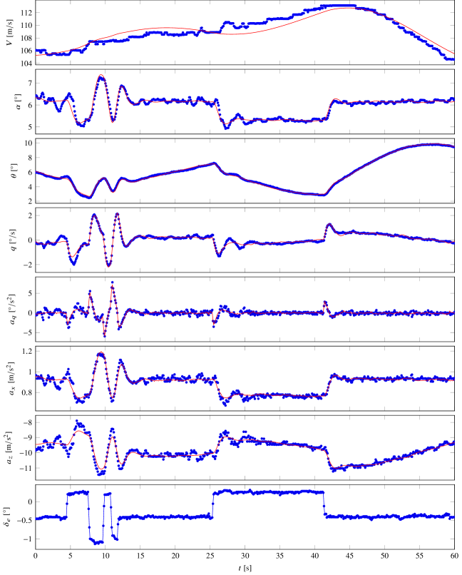
Figure 1: Estimation results for the HFB320 data. The marks are the measured values and the solid lines are the estimated model output. The elevator input for the manuever is the bottommost plot.

parameter	lower starting value	upper starting value	optimal
$C_{D_{0}}$	$0$	$0.5$	$0$	$.0580$
$C_{D_{V}}$	$-0.5$	$0.5$	$-0$	$.0316$
$C_{D_{\alpha}}$	$0$	$1$	$0$	$.2453$
$C_{L_{0}}$	$0$	$2$	$0$	$.1808$
$C_{L_{V}}$	$-2$	$2$	$0$	$.2012$
$C_{L_{\alpha}}$	$0$	$10$	$3$	$.0904$
$C_{m_{0}}$	$0$	$0.5$	$0$	$.1184$
$C_{m_{V}}$	$0$	$0.5$	$0$	$.0137$
$C_{m_{\alpha}}$	$-5$	$1$	$-0$	$.9941$
$C_{m_{q}}$	$-50$	$0$	$-28$	$.6517$
$C_{m_{\delta_{e}}}$	$-10$	$0$	$-1$	$.4714$

Table 3: Limits of the uniform distribution from which the starting parameters of the HFB-320 example were drawn, together with their optimal values.

The estimation was performed a total of $1000$ times with random starting values for the stability and control derivatives, drawn from uniform distributions whose intervals are shown in Tab. 3. The starting value for the bias parameters were zero and for the noise standard deviations was one. The mesh states were initialized with the measured values. Of all starting points of the optimization, $98.6\text{\,}\%$ converged to the global optimum whose parameter values are listed in the last column of Tab. 3 and model outputs are shown in Fig. 1.

We note that the optimization converges even for very bad values of $\theta$ which pose problems for the single shooting implementation. Particularly, if we set all aerodynamic derivatives to zero, there is no lift, drag or aerodynamic pitching moment and the model plummets down, its initial-value problem simulation diverging. However, the collocation-based estimation manages to reach the optimal solution.

3.2 Simulated unstable aircraft short period

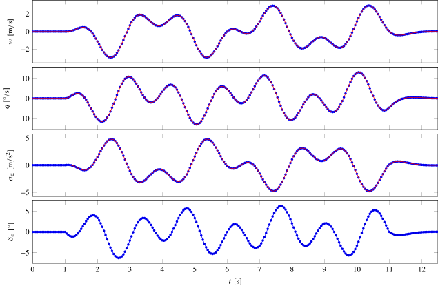
Figure 2: Estimation results for the simulted unstable aircraft data. The marks are the measured values and the solid lines are the estimated model output. The elevator input for the manuever is the bottommost plot.

To demonstrate that the collocation-based output-error method can be used without modifications to estimate unstable dynamics, we apply it on data from an unstable simulated aircraft. The data was used by Jategaonkar [11, Sec. 9.16.1] to compare various methods for unstable aircraft system identification. It should be noted that, for this system, the initial-value problem approach for the output-error method obtains very poor estimates.

A linear model of the short period dynamics was used with 2 states, the vertical velocity $w$ and pitch rate $q$; only 1 input, the elevator deflection $\delta_{e}$; and 3 outputs, $\tilde{w}$, $\tilde{q}$, and the vertical acceleration $\tilde{a}_{z}$. A total of 11 parameters were estimated, the dimensional stability and control derivatives $Z_{w}$, $Z_{q}$, $Z_{\delta_{e}}$, $M_{w}$, $M_{q}$, and $M_{\delta_{e}}$; the measurement noise standard deviations $\sigma_{w}$, $\sigma_{q}$, and $\sigma_{a_{z}}$; and the initial states $w_{0}$ and $q_{0}$.

The system dynamics is defined by

$$\dot{w} =Z_{w}w+(U_{0}+Z_{q})q+Z_{\delta_{e}}\delta_{e}, \dot{q} =M_{w}w+M_{q}q+M_{\delta_{e}}\delta_{e},$$ (43)

and its outputs by

$$\tilde{w} =w, \tilde{q} =q, \tilde{a}_{z} =Z_{w}w+Z_{q}q+Z_{\delta_{e}}\delta_{e}.$$ (44)

The $\ell_{\mathrm{e}}$ log-density associated with Gaussian noise (11) was used, with a diagonal $R(\theta)$ consisting of the measurement variances $\sigma_{w}^{2}$ to $\sigma_{a_{z}}^{2}$. The starting mesh states were the measured values, the stability and control derivatives were zero, and the measurement noise standard deviations were one. The estimation model outputs for the collocation-based output-error method are shown in Fig. 2.

3.3 Black-box high-order ground vibration test

For the estimation of models of the rigid-body flight dynamics of aircraft, most states are measured directly and the model structure is well-known. The estimation of flexible aircraft dynamics poses additional challenges as the structural states are not usually measured and the model order is much larger. Many of these issues also arise in the system identification of structural models from ground vibration tests. To illustrate the application of the collocation-based output-error method to this class of problems, it was applied to accelerometer data from a ground vibration test reported by Gupta et al. [26], part of the Performance Adaptive Aeroelastic Wing program.

A single-input single-output model with 24 states was estimated for the force input $u$ and acceleration output $y$. The dynamics were represented in the state-space modal form:

$$\dot{x}_{1a} =\sigma_{1}x_{1a}+\omega_{1}x_{1b}+b_{1}u$$ (45)

$$\dot{x}_{1b} =-\omega_{1}x_{1a}+\sigma_{1}x_{1b}$$ (46)

$$\;\;\vdots$$ (47)

$$\dot{x}_{12a} =\sigma_{12}x_{12a}+\omega_{12}x_{12b}+b_{12}u$$ (48)

$$\dot{x}_{12b} =-\omega_{12}x_{12a}+\sigma_{12}x_{12b},$$ (49)

such that the system poles are located at $\sigma_{i}\pm j\omega_{i}$. The system output equation is

$$y=c_{1a}x_{1a}+c_{1b}x_{1b}+\dots+c_{12a}x_{12a}+c_{12b}x_{12b}.$$ (50)

The $\ell_{\mathrm{e}}$ log-density associated with Gaussian noise (11) was used, with $R(\theta)=\sigma^{2}_{y}$. The unknown parameter vector consists of the pole locations $\sigma_{i}$ and $\omega_{i}$, the measurement standard deviation $\sigma_{y}$, and the coefficients $b_{i}$, $c_{ia}$, and $c_{ib}$.

$\omega_{1}$	$\omega_{2}$	$\omega_{3}$	$\omega_{4}$	$\omega_{5}$	$\omega_{6}$
$199.06$	$186.17$	$178.44$	$172.64$	$144.37$	$121.47$

$\omega_{7}$	$\omega_{8}$	$\omega_{9}$	$\omega_{10}$	$\omega_{11}$	$\omega_{12}$
$96.52$	$59.57$	$58.57$	$59.03$	$48.99$	$48.90$

Table 4: Starting values for the pole frequencies in the ground vibration test example.

The data collected contains high-frequency components which we do not wish to consider, so both the input and output were filtered with band-pass filters with a passband of $6\text{\,}\mathrm{H}\mathrm{z}32\text{\,}\mathrm{H}\mathrm{z}$, composed of cascaded 5th-order Butterworth filters. The data was then decimated by 20 for the estimation, dropping the sampling rate from $2\text{\,}\mathrm{k}\mathrm{H}\mathrm{z}$ to $100\text{\,}\mathrm{H}\mathrm{z}$. The starting value for the parameters was zero for the $\sigma_{i}$ and mesh states, one for the $c_{ia}$, $c_{ib}$ and $b_{i}$. The starting values of the $\omega_{i}$ were obtained from the poles of a model identified with the N4SID algorithm which are shown in Tab. 4.

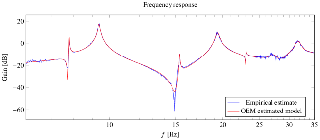
Figure 3: Frequency response magnitude of the empirical transfer function estimate and of the OEM-estimated model for the ground vibration test.

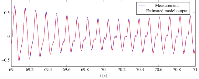
Figure 4: Portion of the time-response of the identified model in the ground vibration test example.

The frequency response of the identified model is shown in Fig. 3, together with that of the empirical transfer function estimate from the test data. A portion of the estimated model outputs shown against the data can also be seen in Fig. 4.

4 Conclusions and future work

The collocation-based output-error method for parameter estimation, although seldomly used in aircraft system identification, better exploits the nature of the inverse problem and has advantages over the ubiquitous single shooting implementations: applicability to a wider class of systems, such as unstable, marginally stable or poorly damped systems; better numerical and convergence properties such as robustness against poor parameter values; parallelizable formulation of the objective function and constraints which can benefit from modern computer hardware and capabilities such as single instruction, multiple data (SIMD), multicore central processing units (CPUs), graphics processing units (GPUs) and computer clusters. These properties can help overcome the challenges in demanding applications like the identification of flexible aircraft dynamics which pose difficulties to the single shooting method.

We note, however, that the main principle behind the collocation method is fairly general: augmenting the optimization decision variables with the states and encoding their dynamics as equality constraints. This overall technique can also be applied to other more general parameter estimation methods as well, notably the filter-error method, lending it similar improvements as for the output-error method.

References

- Ljung [2010] Ljung, L., “Perspectives on system identification,” Annual Reviews in Control, Vol. 34, No. 1, 2010, pp. 1–12. 10.1016/j.arcontrol.2009.12.001.
- Åström and Torsten [1965] Åström, K. J., and Torsten, B., “Numerical Identification of Linear Dynamic Systems from Normal Operating Records,” IFAC Proceedings Volumes, Vol. 2, No. 2, 1965, pp. 96–111. 10.1016/S1474-6670(17)69024-4.
- Åström and Eykhoff [1971] Åström, K. J., and Eykhoff, P., “System identification—A survey,” Automatica, Vol. 7, No. 2, 1971, pp. 123–162. 10.1016/0005-1098(71)90059-8.
- Ljung [1999] Ljung, L., System Identification: Theory for the User, 2nd ed., Prentice Hall, Englewood Cliffs, New Jersey, 07632, 1999.
- Klein [1989] Klein, V., “Estimation of aircraft aerodynamic parameters from flight data,” Progress in Aerospace Sciences, Vol. 26, No. 1, 1989, pp. 1–77. 10.1016/0376-0421(89)90002-X.
- Hamel and Jategaonkar [1996] Hamel, P. G., and Jategaonkar, R. V., “Evolution of Flight Vehicle System Identification,” Journal of Aircraft, Vol. 33, No. 1, 1996, pp. 9–28. 10.2514/3.46898.
- Wang and Iliff [2004] Wang, K. C., and Iliff, K. W., “Retrospective and Recent Examples of Aircraft Parameter Identification at NASA Dryden Flight Research Center,” Journal of Aircraft, Vol. 41, No. 4, 2004, pp. 752–764. 10.2514/1.332.
- Morelli and Klein [2005] Morelli, E. A., and Klein, V., “Application of System Identification to Aircraft at NASA Langley Research Center,” Journal of Aircraft, Vol. 42, No. 1, 2005, pp. 12–25. 10.2514/1.3648.
- Jategaonkar et al. [2004] Jategaonkar, R., Fischenberg, D., and von Gruenhagen, W., “Aerodynamic Modeling and System Identification from Flight Data—Recent Applications at DLR,” Journal of Aircraft, Vol. 41, No. 4, 2004, pp. 681–691. 10.2514/1.3165.
- Klein and Morelli [2006] Klein, V., and Morelli, E., Aircraft System Identification: Theory and Practice, No. 213 in AIAA Education Series, AIAA, 1801 Alexander Bell Drive, Reston, VA 20191, 2006.
- Jategaonkar [2015] Jategaonkar, R. V., Flight Vehicle System Identification: A Time-Domain Methodology, 2nd ed., No. 216 in Progress in Astronautics and Aeronautics, AIAA, 1801 Alexander Bell Drive, Reston, VA 20191, 2015. 10.2514/4.102790.
- Mulder et al. [1999] Mulder, J. A., Chu, Q. P., Sridhar, J. K., Breeman, J. H., and Laban, M., “Non-linear aircraft flight path reconstruction review and new advances,” Progress in aerospace sciences, Vol. 35, No. 7, 1999, pp. 673–726. 10.1016/S0376-0421(99)00005-6.
- Silva and Mönnich [2011] Silva, B. G. O., and Mönnich, W., “Data Gathering and Preliminary Results of the System Identification of a Flexible Aircraft Model,” AIAA Atmospheric Flight Mechanics Conference, 2011. 10.2514/6.2011-6355.
- Silva and Mönnich [2012] Silva, B. G. O., and Mönnich, W., “System Identification of Flexible Aircraft in Time Domain,” AIAA Atmospheric Flight Mechanics Conference, 2012. 10.2514/6.2012-4412.
- Jategaonkar and Thielecke [1994] Jategaonkar, R. V., and Thielecke, F., “Evaluation of Parameter Estimation Methods for Unstable Aircraft,” Journal of Aircraft, Vol. 31, No. 3, 1994, pp. 510–519. 10.2514/3.46523.
- Swartz and Bremermann [1975] Swartz, J., and Bremermann, H., “Discussion of parameter estimation in biological modelling: Algorithms for estimation and evaluation of the estimates,” Journal of Mathematical Biology, Vol. 1, No. 3, 1975, pp. 241–257. 10.1007/BF01273746.
- Bock [1981] Bock, H. G., “Numerical Treatment of Inverse Problems in Chemical Reaction Kinetics,” Modelling of Chemical Reaction Systems, Springer Series in Chemical Physics, Vol. 18, edited by K. H. Ebert, P. Deuflhard, and W. Jäger, Springer, Berlin, Heidelberg, 1981, pp. 102–125. 10.1007/978-3-642-68220-9_8.
- Bock [1983] Bock, H. G., “Recent Advances in Parameteridentification Techniques for O.D.E.” Numerical Treatment of Inverse Problems in Differential and Integral Equations, Progress in Scientific Computing, Vol. 2, edited by P. Deuflhard and E. Hairer, Birkhäuser Boston, 1983, pp. 95–121. 10.1007/978-1-4684-7324-7_7.
- Schlöder and Bock [1982] Schlöder, J., and Bock, H. G., “Identification of Rate Constants in Bistable Chemical Reactions,” Numerical Treatment of Inverse Problems in Differential and Integral Equations, Progress in Scientific Computing, Vol. 2, edited by P. Deuflhard and E. Hairer, Birkhäuser Boston, 1982, pp. 27–47. 10.1007/978-1-4684-7324-7_3.
- Lohmann et al. [1992] Lohmann, T., Bock, H. G., and Schloeder, J. P., “Numerical Methods for Parameter Estimation and Optimal Experiment Design in Chemical Reaction Systems,” Industrial & Engineering Chemistry Research, Vol. 31, 1992, pp. 54–57. 10.1021/ie00001a008.
- Betts [2010] Betts, J. T., Practical methods for optimal control and estimation using nonlinear programming, 2nd ed., Advances in Design and Control, SIAM, 2010. 10.1137/1.9780898718577.
- Bock and Plitt [1984] Bock, H. G., and Plitt, K. J., “A Multiple Shooting Algorithm for Direct Solution of Optimal Control Problems,” IFAC Proceedings Volumes, Vol. 17, No. 2, 1984, pp. 1603–1608. 10.1016/S1474-6670(17)61205-9.
- Dutra et al. [2014] Dutra, D. A., Teixeira, B. O. S., and Aguirre, L. A., “Maximum a posteriori state path estimation: Discretization limits and their interpretation,” Automatica, Vol. 50, No. 5, 2014, pp. 1360–1368. 10.1016/j.automatica.2014.03.003.
- Dutra et al. [2017] Dutra, D. A. A., Teixeira, B. O. S., and Aguirre, L. A., “Joint maximum a posteriori state path and parameter estimation in stochastic differential equations,” Automatica, 2017, pp. 403–408. 10.1016/j.automatica.2017.03.035.
- Grauer and Boucher [2018] Grauer, J. A., and Boucher, M. J., “Real-Time Parameter Estimation for Flexible Aircraft,” AIAA Atmospheric Flight Mechanics Conference, 2018. 10.2514/6.2018-3155.
- Gupta et al. [2016] Gupta, A., Seiler, P. J., and Danowsky, B. P., “Ground Vibration Tests on a Flexible Flying Wing Aircraft,” AIAA Atmospheric Flight Mechanics Conference, American Institute of Aeronautics and Astronautics, 2016. 10.2514/6.2016-1753.
- Aravkin et al. [2012a] Aravkin, A., Burke, J., and Pillonetto, G., “Nonsmooth regression and state estimation using piecewise quadratic log-concave densities,” IEEE CDC, 2012a, pp. 4101–4106. 10.1109/CDC.2012.6426893.
- Aravkin et al. [2012b] Aravkin, A., Burke, J., and Pillonetto, G., “Robust and Trend-Following Kalman Smoothers Using Student’s t,” SYSID, 2012b, pp. 1215–1220. 10.3182/20120711-3-BE-2027.00283.
- Aravkin et al. [2012c] Aravkin, A., Burke, J., and Pillonetto, G., “A Statistical and Computational Theory for Robust and Sparse Kalman Smoothing,” SYSID, 2012c, pp. 894–899. 10.3182/20120711-3-BE-2027.00282.
- Aravkin et al. [2013] Aravkin, A., Burke, J., and Pillonetto, G., “Sparse/Robust Estimation and Kalman Smoothing with Nonsmooth Log-Concave Densities,” J. Mach. Learn. Res., Vol. 14, No. 9, 2013, pp. 2689–2728.
- Aravkin et al. [2017] Aravkin, A., Burke, J. V., Ljung, L., Lozano, A., and Pillonetto, G., “Generalized Kalman smoothing: Modeling and algorithms,” Automatica, Vol. 86, 2017, pp. 63–86. 10.1016/j.automatica.2017.08.011.
- Shampine [1985] Shampine, L. F., “Interpolation for Runge-Kutta Methods,” SIAM Journal on Numerical Analysis, Vol. 22, No. 5, 1985, pp. 1014–1027. 10.1137/0722060.
- Wächter and Biegler [2006] Wächter, A., and Biegler, L. T., “On the implementation of an interior-point filter line-search algorithm for large-scale nonlinear programming,” Mathematical Programming, Vol. 106, No. 1, 2006, pp. 25–57. 10.1007/s10107-004-0559-y.
- Betts and Huffman [2003] Betts, J., and Huffman, W., “Large Scale Parameter Estimation Using Sparse Nonlinear Programming Methods,” SIAM Journal on Optimization, Vol. 14, No. 1, 2003, pp. 223–244. 10.1137/S1052623401399216.
- Williams and Trivailo [2005] Williams, P., and Trivailo, P., “Optimal parameter estimation of dynamical systems using direct transcription methods,” Inverse Problems in Science and Engineering, Vol. 13, No. 4, 2005, pp. 377–409. 10.1080/17415970500104499.
- Wang et al. [2013] Wang, Q., Zhang, X., Zhang, Y., and Yi, Q., “AUGEM: Automatically Generate High Performance Dense Linear Algebra Kernels on x86 CPUs,” Proceedings of the International Conference on High Performance Computing, Networking, Storage and Analysis, ACM, New York, NY, USA, 2013, pp. 25:1–25:12. 10.1145/2503210.2503219.
- OpenMP Architecture Review Board [2013] OpenMP Architecture Review Board, “OpenMP Application Program Interface Version 4.0,” , July 2013.