Consensus of the Hegselmann-Krause opinion
formation model with time delay

Abstract

In this paper, we study Hegselmann–Krause models with a time-variable time delay. Under appropriate assumptions, we show the exponential asymptotic consensus when the time delay satisfies a suitable smallness assumption. Our main strategies for this are based on Lyapunov functional approach and careful estimates on the trajectories. We then study the mean-field limit from the many-individual Hegselmann–Krause equation to the continuity-type partial differential equation as the number $N$ of individuals goes to infinity. For the limiting equation, we prove global-in-time existence and uniqueness of measure-valued solutions. We also use the fact that constants appearing in the consensus estimates for the particle system are independent of $N$ to extend the exponential consensus result to the continuum model. Finally, some numerical tests are illustrated.

1 Introduction

Recently, multi-agent models have attracted the interest of many authors in several scientific disciplines. A particularly interesting aspect of the dynamics of multi-agent systems is the natural self-organization which leads to the emergence of a globally collective behavior. This happens for biological systems [5, 16], physical systems [33], ecosystems [32], social sciences [2, 3, 11, 31]. We also mention engineering applications [4, 17, 23], economics models [21, 26], control problems [1, 28, 34]. Various models have been proposed to study opinion dynamics [11, 18, 21, 24, 35].

It is also natural to include a time delay in the model. Time delay effects frequently appear in applications, in biological and physical models, as well as in social dynamics, economics and control problems. Indeed, a certain time is needed for each agent to receive information from other agents. Also, a time lag can appear in the evolution of a multi-agent system as a reaction time. In the current work, we are interested in the so–called Hegselmann–Krause model (see [21]) and study the opinion formation in the presence of a time-variable time delay, see also [25] for a model with constant interaction rates and constant delay. Among other results about Hegselmann–Krause type models without time delays, we refer to [12, 22], where clusters formation is studied in case of bounded confidence. For second–order consensus models, in particular Cucker–Smale type models with time delays, we refer to recent papers [13, 14, 15, 19, 20, 29, 30].

Let $x_{i}\in{{\rm I}\kern-1.49994pt{\rm R}}^{d}$ represent an opinion of $i$-th agent, then our main system reads as

$$\frac{dx_{i}(t)}{dt}=\frac{\lambda}{N}\sum_{j\neq i}a_{ij}(t)(x_{j}(t-\tau(t))-x_{i}(t)),\quad i=1,\dots,N,\quad t>0,$$ (1.1)

with initial data given by

$$x_{i}(s)=x_{i,0}(s),\quad\forall\,s\in[-\tau(0),0],$$ (1.2)

where the coupling strength $\lambda$ is a positive parameter and the communication rates $a_{ij}(t)$ are of the form

$$a_{ij}(t)=\psi(|x_{j}(t-\tau(t))-x_{i}(t)|),$$ (1.3)

with $\psi:[0,+\infty)\rightarrow(0,+\infty)$ non-increasing function or, in the spirit of [27],

$$a_{ij}(t)=\frac{N\psi(|x_{j}(t-\tau(t))-x_{i}(t)|)}{\sum_{k=1}^{N}\psi(|x_{k}(t-\tau(t))-x_{i}(t)|)}$$ (1.4)

with $\psi$ as above. Without loss of generality, we assume $\psi(0)=1.$ Note that in both cases we have, for $i=1,\dots,N,$

$$\frac{1}{N}\sum_{j=1}^{N}a_{ij}(t)\leqslant 1,\quad\forall\,t\geqslant 0.$$ (1.5)

The time delay $\tau(\cdot)$ is a positive function belonging to $W^{1,\infty}_{loc}(0,+\infty)$ and satisfying

$$0\leq\tau(t)\leq\overline{\tau},\quad\forall\,t>0,$$ (1.6)

and

$$\tau^{\prime}(t)\leq c,\quad c\in(0,1),\quad\forall\,t>0.$$ (1.7)

Now, we define the position diameter as follows:

$$d_{X}(t):=\max_{1\leqslant i,j\leqslant N}|x_{i}(t)-x_{j}(t)|.$$ (1.8)

Definition 1.1.

We say that the dynamics, subject to (1.1), converges to consensus if

$$d_{X}(t)\rightarrow 0\quad\mbox{\rm as}\quad t\rightarrow+\infty.$$

By constructing a suitable Lyapunov functional, in the first part of our work, we will deduce exponential consensus estimates when the time delay is sufficiently small. Note that the constants in the decay estimates are independent of the number of the agents; this is crucial in order to extend the consensus estimate for the associated continuum equation below.

In the second part of the paper, we will study the continuum model obtained as mean-field limit of the particle system when $N\rightarrow\infty.$ Let $\mathcal{M}({{\rm I}\kern-1.49994pt{\rm R}}^{d})$ be the set of probability measures on the space ${{\rm I}\kern-1.49994pt{\rm R}}^{d}$. Then, the continuum model associated to the particle system (1.1) is given by

$$\begin{aligned} &\partial_{t}\mu_{t}+\mbox{\rm div}\ (F[\mu_{t-\tau(t)}]\mu_{t})=0,\quad x\in{{\rm I}\kern-1.49994pt{\rm R}}^{d},\quad t>0,\cr&\mu_{s}=:g_{s},\quad x\in{{\rm I}\kern-1.49994pt{\rm R}}^{d},\quad s\in[-\tau(0),0],\end{aligned}$$ (1.9)

where the velocity field $F$ is given by either

$$F[\mu_{t-\tau(t)}](x)=\int_{{{\rm I}\kern-1.04996pt{\rm R}}^{d}}\psi(|x-y|)(y-x)\,d\mu_{t-\tau(t)}(y),$$ (1.10)

or

$$F[\mu_{t-\tau(t)}](x)=\displaystyle{\frac{\int_{{{\rm I}\kern-1.04996pt{\rm R}}^{d}}\psi(|x-y|)(y-x)\,d\mu_{t-\tau(t)}(y)}{\int_{{{\rm I}\kern-1.04996pt{\rm R}}^{d}}\psi(|x-y|)\,d\mu_{t-\tau(t)}(y)},}$$ (1.11)

according to (1.3) and (1.4), and $g_{s}\in\mathcal{C}([-\tau(0),0];\mathcal{M}({{\rm I}\kern-1.49994pt{\rm R}}^{d}))$. For the derivation of the continuum model associated to the Hegselmann–Krause system, without time delays, we refer to [7]. Since then, kinetic formulations for opinion dynamics have been the objects of several works, see e.g [6, 8, 10, 28]. On the other hand, the continuum formulation in presence of delay effects seems new.

Following a similar strategy to the one used for the kinetic Cucker-Smale equation in [13] (see also [15]) we will study the global-in-time well–posedness of (1.9), more precisely, global existence and uniqueness of measure-valued solutions. In addition, we prove a stability estimate which allows to rigorously justify the mean–field limit procedure. Furthermore, the stability estimate, together with the uniform-in-$N$ consensus estimate for the particle model, enables us to extend the asymptotic consensus to the continuum equation.

The rest of this paper is organized as follows. In Sect. 2, we will study the particle model (1.1) and show the consensus behavior for small delays. In Sect. 3, we will focus on the continuum model (1.9) obtained formally from the particle system, and we will analyze it in the set of the probability measures employing the Wasserstein distance of order $p\in[1,\infty]$. Finally, some numerical simulations are illustrated in Sect. 4.

2 Exponential consensus behavior of the particle system

In order to study the convergence to consensus of system (1.1)-(1.2), we need some auxiliary lemmas.

Lemma 2.1.

Let $\{x_{i}\}_{i=1}^{N}$ be a solution to (1.1)-(1.2). Suppose that the initial opinions $x_{i,0}(s)$ are continuous functions of $s\in[-\tau(0),0]$. Moreover, let us denote

$$R=\max_{s\in[-\tau(0),0]}\max_{1\leqslant i\leqslant N}|x_{i}(s)|.$$

Then we have

$$R_{X}(t):=\max_{1\leqslant i\leqslant N}|x_{i}(t)|\leqslant R,\quad\forall t\in[-\tau(0),+\infty).$$

Proof.

For any $\epsilon>0$, let us define

$$S^{\epsilon}=\left\{t>0\,:\ R_{X}(s)<R+\epsilon,\ \ s\in[0,t)\right\}.$$

Let us denote $T^{\epsilon}_{*}:=\sup S^{\epsilon}.$ By continuity, $S^{\epsilon}\neq\emptyset$. Hence, $T_{*}>0$. We claim that $T_{*}^{\epsilon}=+\infty.$ To prove this we argue by contradiction. Suppose that $T_{*}^{\epsilon}<+\infty.$ Then,

$$\lim_{t\rightarrow T_{*}^{\epsilon-}}R_{X}(t)=R+\epsilon\quad\text{and}\quad R_{X}(t)<R+\epsilon,\quad\forall t<T_{*}^{\epsilon}.$$ (2.12)

Now, for $t<T_{*}^{\epsilon}$, we can compute

$$\frac{1}{2}\frac{d}{dt}|x_{i}(t)|^{2} =\left\langle x_{i},\frac{\lambda}{N}\sum_{j\neq i}a_{ij}(t)(x_{j}(t-\tau(t))-x_{i}(t))\right\rangle$$

$$=\frac{\lambda}{N}\sum_{j\neq i}a_{ij}(t)\Bigl{(}\langle x_{i}(t),x_{j}(t-\tau(t))\rangle-|x_{i}(t)|^{2}\Bigr{)}$$

$$\leqslant\frac{\lambda}{N}\sum_{j\neq i}a_{ij}(t)|x_{i}(t)|\Bigl{(}|x_{j}(t-\tau(t))|-|x_{i}(t)|\Bigr{)}$$

$$\leqslant\frac{\lambda}{N}\sum_{j\neq i}a_{ij}(t)\Bigl{(}R+{\epsilon}-|x_{i}(t)|\Bigr{)}|x_{i}(t)|.$$

Then, we deduce

$$\frac{d}{dt}|x_{i}(t)|\leq\frac{\lambda}{N}\sum_{j\neq i}a_{ij}(t)\Bigl{(}R+{\epsilon}-|x_{i}(t)|\Bigr{)},$$

and so, recalling (1.5), we have

$$\frac{d}{dt}|x_{i}(t)|\leqslant\lambda(R+\epsilon-|x_{i}(t)|).$$

Hence, Gronwall's inequality yields the estimate

$$|x_{i}(t)|\leqslant e^{-\lambda t}\Bigl{(}|x_{i}(0)|-R-\epsilon\Bigr{)}+R+\epsilon<R+\epsilon.$$ (2.13)

From (2.13) we deduce $\lim_{t\rightarrow T_{*}^{\epsilon}}R_{X}(t)<R+\epsilon$, which is in contradiction with (2.12). Being $\epsilon$ arbitrary, the lemma is proved.    

Remark 2.2.

From Lemma 2.1, we have that for $i,j=1,\dots,N,$

$$|x_{j}(t-\tau(t))-x_{i}(t)|\leqslant|x_{j}(t-\tau(t))|+|x_{i}(t)|\leqslant 2R,\quad\forall\,t\geq 0.$$

So, from (1.3) and (1.4), we deduce

$$a_{ij}(t)\geqslant\psi(2R),\quad\forall\ t\geq 0.$$ (2.14)

The diameter function $d_{X}$ is not differentiable in general. Thus, we introduce the upper Dini derivative to consider the time derivative of this function. For a given continuous function $F=F(t)$, the upper Dini derivative of $F$ at $t$ is defined by

$$D^{+}F(t):=\limsup_{h\to 0^{+}}\frac{F(t+h)-F(t)}{h}.$$

Note that the Dini derivative coincides with the usual derivative when the function is differentiable at $t$.

Then we have the following lemma.

Lemma 2.3.

Let $\{x_{i}\}_{i=1}^{N}$ be a solution to (1.1)-(1.2). If

$$\sigma_{\tau}(t):=\int_{t-\tau(t)}^{t}\max_{1\leqslant k\leqslant N}|\dot{x}_{k}(s)|\,ds,$$

then the position diameter $d_{X}(\cdot)$ satisfies

$$D^{+}d_{X}(t)\leqslant\frac{2\lambda}{\psi(2R)}\sigma_{\tau}(t)-\lambda\psi(2R)d_{X}(t),\quad\forall\,t\geqslant 0.$$

Proof.

Due to the continuity of the trajectories $x_{i}(t),$ $i=1,\dots,N,$ there is an at most countable system of open disjoint intervals $\{\mathcal{I}_{\delta}\}_{\delta\in\mathbb{N}}$ such that

$$\bigcup_{\delta\in\mathbb{N}}\overline{\mathcal{I}_{\delta}}=[0,\infty)$$

and for each ${\delta\in\mathbb{N}}$ there exist indices $i(\delta)$, $j(\delta)$ such that

$$d_{X}(t)=|x_{i(\delta)}(t)-x_{j(\delta)}(t)|,\quad t\in\mathcal{I}_{\delta}.$$

For simplicity of notation, we can put $i:=i(\delta)$, $j:=j(\delta).$ Of course, we can assume $i\neq j.$ For $t\in\mathcal{I}_{\delta}$, we have

$$\begin{array}[]{l}\displaystyle{\frac{1}{2}D^{+}d_{X}^{2}(t)}\\ \hskip 14.22636pt\displaystyle{=\frac{\lambda}{N}\Big{\langle}x_{i}(t)-x_{j}(t),\sum_{k\neq i}a_{ik}(t)(x_{k}(t-\tau(t))-x_{i}(t))-\sum_{k\neq j}a_{jk}(t)(x_{k}(t-\tau(t))-x_{j}(t))\Big{\rangle}}\\ \displaystyle{\hskip 14.22636pt=\frac{\lambda}{N}\sum_{k\neq i}a_{ik}(t)\langle x_{i}(t)-x_{j}(t),x_{k}(t-\tau(t))-x_{i}(t)\rangle}\\ \hskip 71.13188pt\displaystyle{-\frac{\lambda}{N}\sum_{k\neq j}a_{jk}(t)\langle x_{i}(t)-x_{j}(t),x_{k}(t-\tau(t))-x_{j}(t)\rangle}\\ \hskip 14.22636pt=:I_{1}+I_{2}.\end{array}$$ (2.15)

Now, we can rewrite $I_{1}$ and $I_{2}$ as

$$\begin{array}[]{l}\displaystyle{I_{1}=\frac{\lambda}{N}\sum_{k\neq i}a_{ik}(t)\langle x_{i}(t)-x_{j}(t),x_{k}(t-\tau(t))-x_{k}(t)\rangle}\\ \displaystyle{\hskip 28.45274pt+\frac{\lambda}{N}\sum_{k\neq i}a_{ik}(t)\langle x_{i}(t)-x_{j}(t),x_{k}(t)-x_{i}(t)\rangle}\quad\mbox{and}\end{array}$$ (2.16)

$$\begin{array}[]{l}\displaystyle{I_{2}=-\frac{\lambda}{N}\sum_{k\neq j}a_{jk}(t)\langle x_{i}(t)-x_{j}(t),x_{k}(t-\tau(t))-x_{k}(t)\rangle}\\ \displaystyle{\hskip 28.45274pt-\frac{\lambda}{N}\sum_{k\neq j}a_{jk}(t)\langle x_{i}(t)-x_{j}(t),x_{k}(t)-x_{j}(t)\rangle,}\end{array}$$

respectively. We observe that for all$k=1,\dots,N,$

$$\langle x_{i}(t)-x_{j}(t),x_{k}(t)-x_{i}(t)\rangle\leqslant 0.$$

Indeed, using Cauchy-Schwartz inequality, we have that

$$\langle x_{i}(t)-x_{j}(t),x_{k}(t)-x_{i}(t)\rangle =\langle x_{i}(t)-x_{j}(t),x_{k}(t)-x_{j}(t)\rangle-|x_{i}(t)-x_{j}(t)|^{2}$$

$$\leqslant|x_{i}(t)-x_{j}(t)|\left(|x_{k}(t)-x_{j}(t)|-|x_{i}(t)-x_{j}(t)|\right)$$

$$\leqslant 0.$$

Now, observe that in both cases (1.3) and (1.4),

$$a_{ik}(t)\leqslant\frac{1}{\psi(2R)},\quad\forall\ t\geq 0.$$ (2.17)

Hence, using (2.14) and (2.17) in (2.16), we obtain

$$I_{1}\leqslant\frac{\lambda}{N}\frac{d_{X}(t)}{\psi(2R)}\sum_{k=1}^{N}|x_{k}(t-\tau(t))-x_{k}(t)|+\frac{\lambda}{N}{\psi(2R)}\sum_{k=1}^{N}\langle x_{i}(t)-x_{j}(t),x_{k}(t)-x_{i}(t)\rangle.$$ (2.18)

Now, observe that

$$-\langle x_{i}(t)-x_{j}(t),x_{k}(t)-x_{j}(t)\rangle\leqslant 0,\quad\forall\ k=1,\dots,N.$$

Then, arguing analogously to before, one can estimate

$$I_{2}\leqslant\frac{\lambda}{N}\frac{d_{X}(t)}{\psi(2R)}\sum_{k=1}^{N}|x_{k}(t-\tau(t))-x_{k}(t)|-\frac{\lambda}{N}\psi(2R)\sum_{k=1}^{N}\langle x_{i}(t)-x_{j}(t),x_{k}(t)-x_{j}(t)\rangle.$$ (2.19)

Therefore, using (2.18) and (2.19) in (2.15), we obtain

$$\frac{1}{2}D^{+}d_{X}^{2}(t)\leqslant 2\frac{\lambda}{N}\frac{d_{X}(t)}{\psi(2R)}\sum_{k=1}^{N}|x_{k}(t-\tau(t))-x_{k}(t)|-\lambda\psi(2R)d_{X}^{2}(t),$$

and so

$$D^{+}d_{X}(t)\leqslant 2\frac{\lambda}{N\psi(2R)}\sum_{k=1}^{N}|x_{k}(t-\tau(t))-x_{k}(t)|-\lambda\psi(2R)d_{X}(t).$$ (2.20)

Noticing that

$$\sum_{k=1}^{N}|x_{k}(t-\tau(t))-x_{k}(t)| \leqslant\sum_{k=1}^{N}\int_{t-\tau(t)}^{t}|\dot{x}_{k}(s)|\,ds$$

$$\leqslant N\sigma_{\tau}(t),$$

then from (2.20) we obtain

$$D^{+}d_{X}(t)\leqslant\frac{2\lambda}{\psi(2R)}\sigma_{\tau}(t)-\lambda\psi(2R)d_{X}(t),$$

which proves the lemma.    

Lemma 2.4.

Let $\{x_{i}\}_{i=1}^{N}$ be a solution to (1.1)-(1.2). Then, we have

$$\max_{1\leqslant i\leqslant N}|\dot{x}_{i}(t)|\leqslant\frac{\lambda}{\psi(2R)}\sigma_{\tau}(t)+\frac{\lambda}{\psi(2R)}d_{X}(t).$$ (2.21)

Proof.

A straightforward computation gives

$$|\dot{x}_{i}(t)| =\left|\frac{\lambda}{N}\sum_{j\neq i}a_{ij}(t)(x_{j}(t-\tau(t))-x_{j}(t))+\frac{\lambda}{N}\sum_{j\neq i}a_{ij}(t)(x_{j}(t)-x_{i}(t))\right|$$

$$\leqslant\frac{\lambda}{N}\sum_{j\neq i}a_{ij}(t)|x_{j}(t-\tau(t))-x_{j}(t)|+\frac{\lambda}{N}\sum_{j\neq i}a_{ij}(t)|x_{j}(t)-x_{i}(t)|$$

$$\leqslant\frac{\lambda}{N\psi(2R)}\sum_{j\neq i}\int_{t-\tau(t)}^{t}|\dot{x}_{j}(s)|\,ds+\lambda\frac{N-1}{N\psi(2R)}d_{X}(t)$$

$$\leqslant\lambda\frac{N-1}{N\psi(2R)}\sigma_{\tau}(t)+\lambda\frac{N-1}{N\psi(2R)}d_{X}(t).$$

Taking the maximum for $i\in\{1,\dots,N\},$ we obtain (2.21).    

Theorem 2.5.

Let $\{x_{i}\}_{i=1}^{N}$ be a solution to (1.1)-(1.2). Suppose that

$$\overline{\tau}<\ln\left(1+\frac{\psi^{3}(2R)}{2+\psi^{2}(2R)}\,\frac{1-c}{\lambda}\right).$$

Then, there exist $\gamma,C>0$ such that

$$d_{X}(t)\leqslant Ce^{-\gamma t},\quad\forall\,t\geqslant 0.$$

Proof.

Consider the Lyapunov functional

$$F(t)=d_{X}(t)+\beta\int_{t-\tau(t)}^{t}{e^{-(t-s)}\int_{s}^{t}\max_{1\leqslant j\leqslant N}|\dot{x}_{j}(\sigma)|\,d\sigma}ds.$$

Then, we have

$$D^{+}F(t) =D^{+}d_{X}(t)-\beta(1-\tau^{\prime}(t))e^{-\tau(t)}\int_{t-\tau(t)}^{t}\max_{1\leqslant j\leqslant N}|\dot{x}_{j}(\sigma)|\,d\sigma$$

$$\quad+\beta\int_{t-\tau(t)}^{t}e^{-(t-s)}\max_{1\leqslant j\leqslant N}|\dot{x}_{j}(t)|\,ds$$

$$\quad-\beta\int_{t-\tau(t)}^{t}e^{-(t-s)}\int_{s}^{t}\max_{1\leqslant j\leqslant N}|\dot{x}_{j}(\sigma)|\,d\sigma ds$$

$$\leqslant\left(-\lambda\psi(2R)+(1-e^{-\tau(t)})\frac{\lambda\beta}{\psi(2R)}\right)d_{X}(t)$$

$$\quad+\left(\frac{2\lambda}{\psi(2R)}-\beta(1-\tau^{\prime}(t))e^{-\tau(t)}+\beta(1-e^{-\tau(t)})\frac{\lambda}{\psi(2R)}\right)\sigma_{\tau}(t)$$

$$\quad-\beta\int_{t-\tau(t)}^{t}e^{-(t-s)}\int_{s}^{t}\max_{1\leqslant j\leqslant N}|\dot{x}_{j}(\sigma)|\,d\sigma ds.$$

Hence, from the assumptions (1.6) and (1.7) we deduce

$$D^{+}F(t) \leqslant\left(-\lambda\psi(2R)+(1-e^{-\overline{\tau}})\frac{\lambda\beta}{\psi(2R)}\right)d_{X}(t)$$ (2.22)

$$\quad+\left(\frac{2\lambda}{\psi(2R)}-\beta(1-c)e^{-\overline{\tau}}+\beta(1-e^{-\overline{\tau}})\frac{\lambda}{\psi(2R)}\right)\sigma_{\tau}(t)$$ (2.23)

$$\quad-\beta\int_{t-\tau(t)}^{t}e^{-(t-s)}\int_{s}^{t}\max_{1\leqslant j\leqslant N}|\dot{x}_{j}(\sigma)|\,d\sigma ds.$$ (2.24)

Now, we want to show that for $\overline{\tau}$ sufficiently small we can choose the positive parameter $\beta$ in the definition of the Lyapunov functional $F(\cdot)$ such that (2.22) implies

$$D^{+}F(t)\leq-\gamma F(t),\quad\forall\,t\geqslant 0,$$ (2.25)

for a suitable positive constant $\gamma.$ In order to have (2.25) the following two conditions have to be satisfied:

$$\frac{2\lambda}{\psi(2R)}-\beta(1-c)e^{-\overline{\tau}}+\beta(1-e^{-\overline{\tau}})\frac{\lambda}{\psi(2R)}\leq 0\quad\mbox{and}$$ (2.26)

$$-\psi(2R)+(1-e^{-\overline{\tau}})\frac{\beta}{\psi(2R)}<0.$$ (2.27)

We can rewrite (2.26) as

$${2\lambda}-\beta\psi(2R)(1-c)e^{-\overline{\tau}}+\lambda\beta(1-e^{-\overline{\tau}})\leq 0,$$

which is satisfied for

$$\beta\geq\frac{2\lambda}{\psi(2R)(1-c)e^{-\overline{\tau}}-\lambda(1-e^{-\overline{\tau}})}.$$ (2.28)

This requires a first restriction on the time delay size, i.e.

$$\overline{\tau}<\ln\left(1+\psi(2R)\frac{(1-c)}{\lambda}\right).$$ (2.29)

Condition (2.27) instead implies

$$\beta<\frac{\psi^{2}(2R)}{1-e^{-\overline{\tau}}}.$$ (2.30)

Then, for the existence of a parameter $\beta$ satisfying both (2.28) and (2.30), we need

$$\frac{2\lambda}{\psi(2R)(1-c)e^{-\overline{\tau}}-\lambda(1-e^{-\overline{\tau}})}<\frac{\psi^{2}(2R)}{1-e^{-\overline{\tau}}},$$

and this gives a further condition on $\overline{\tau},$ namely

$$\overline{\tau}<\ln\left(1+\frac{\psi^{3}(2R)}{2+\psi^{2}(2R)}\,\frac{1-c}{\lambda}\right),$$

which clearly implies (2.29). Hence, the theorem is proved.    

Remark 2.6.

Note that in the case of potential communication rates as in (1.3) the estimate (2.17) can be replaced by

$$a_{ij}(t)\leq 1.$$

Therefore, in such a case we can obtain an improved bound on the size of the time delay:

$$\overline{\tau}<\ln\left(1+\frac{\psi}{2+\psi}\frac{1-c}{\lambda}\right).$$

3 The continuum model: measure-valued solutions & consensus behavior

In this section, in the same spirit of [13], we provide the existence, uniqueness of solution to the continuum model (1.9) associated to (1.1) and its consensus behavior under a suitable smallness assumption on the delay function $\tau(t)$.

In order to study the existence and uniqueness of the solution of the continuum model, we assume that the delay function $\tau(\cdot)$ is bounded from below, namely there exists a strictly positive constant $\tau^{*}>0$ such that

$$\tau(t)\geqslant\tau^{*},\quad\forall\,t\geqslant 0.$$

Moreover, we assume that the potential $\psi(\cdot)$ in (1.3) and (1.4) is also Lipschitz continuous, and we denote by $L$ its Lipschitz constant.

We define the Wasserstein distance as follows.

Definition 3.1.

Let $\mu,\nu\in\mathcal{M}({{\rm I}\kern-1.49994pt{\rm R}}^{d})$ be two probability measures on ${{\rm I}\kern-1.49994pt{\rm R}}^{d}$. Then, we define the Wasserstein distance of order $1\leqslant p<\infty$ between $\mu$ and $\nu$ as

$$d_{p}(\mu,\nu):=\inf_{\pi\in\Pi(\mu,\nu)}\left(\int_{{{\rm I}\kern-1.04996pt{\rm R}}^{d}\times{{\rm I}\kern-1.04996pt{\rm R}}^{d}}|x-y|^{p}\,d\pi(x,y)\right)^{1/p}$$

and for $p=\infty$, limiting case as $p\to\infty$,

$$d_{\infty}(\mu,\nu):=\inf_{\pi\in\Pi(\mu,\nu)}\left(\sup_{(x,y)\in\mbox{\small}{supp}(\pi)}|x-y|\right),$$

where $\Pi(\mu,\nu)$ is the set of all probability measures on ${{\rm I}\kern-1.49994pt{\rm R}}^{2d}$ with marginals $\mu$ and $\nu$ (also called couplings for $\mu$ and $\nu$), namely

$$\int_{{{\rm I}\kern-1.04996pt{\rm R}}^{d}\times{{\rm I}\kern-1.04996pt{\rm R}}^{d}}\phi(x)\,d\pi(x,y)=\int_{{{\rm I}\kern-1.04996pt{\rm R}}^{d}}\phi(x)\,d\mu(x),\qquad\int_{{{\rm I}\kern-1.04996pt{\rm R}}^{d}\times{{\rm I}\kern-1.04996pt{\rm R}}^{d}}\phi(y)\,d\pi(x,y)=\int_{{{\rm I}\kern-1.04996pt{\rm R}}^{d}}\phi(y)\,d\nu(y),$$

for all continuous and bounded functions $\phi\in\mathcal{C}_{b}({{\rm I}\kern-1.49994pt{\rm R}}^{d})$.

Note that $\mathcal{P}_{p}({{\rm I}\kern-1.49994pt{\rm R}}^{d})$, which stands for the set of probability measures with bounded moments of order $p\in[1,\infty)$, endowed with the $p$-Wasserstein distance $d_{p}$ is a complete metric space. Moreover, we recall the definiton of the push-forward of a measure:

Definition 3.2.

Let $\mu$ be a Borel measure on ${{\rm I}\kern-1.49994pt{\rm R}}^{d}$ and let $\mathcal{T}:{{\rm I}\kern-1.49994pt{\rm R}}^{d}\rightarrow{{\rm I}\kern-1.49994pt{\rm R}}^{d}$ be a measurable map. Then, we define the push-forward of $\mu$ via $\mathcal{T}$ as the measure given by

$$\mathcal{T}\#\mu(B):=\mu(\mathcal{T}^{-1}(B)),$$

for all Borel sets $B\subset{{\rm I}\kern-1.49994pt{\rm R}}^{d}$.

Furthermore, we define the notion of measure-valued solution to (1.9).

Definition 3.3.

Let $T>0$ be any given time. We say that $\mu_{t}\in\mathcal{C}([0,T);\mathcal{M}({{\rm I}\kern-1.49994pt{\rm R}}^{d}))$ is a measure-valued solution to (1.9) on the time-interval $[0,T)$ if for all $\phi\in\mathcal{C}_{c}^{\infty}({{\rm I}\kern-1.49994pt{\rm R}}^{d}\times[0,T))$ we have that

$$\int_{0}^{T}\int_{{{\rm I}\kern-1.04996pt{\rm R}}^{d}}(\partial_{t}\phi+F[\mu_{t-\tau(t)}](x)\cdot\nabla_{x}\phi)\,d\mu_{t}(x)dt+\int_{{{\rm I}\kern-1.04996pt{\rm R}}^{d}}\phi(x,0)\,dg_{0}(x)=0,$$ (3.31)

where $F[\mu_{t-\tau(t)}]$ is defined as in (1.10) or (1.11).

Let us denote $B^{d}(0,R)$ the ball of radius $R$ in ${{\rm I}\kern-1.49994pt{\rm R}}^{d}$ centered at the origin. In order to prove existence and uniqueness of solution to the kinetic model (1.9), we have the following lemma.

Lemma 3.4.

Let $\mu_{t}\in\mathcal{C}([0,T];\mathcal{M}({{\rm I}\kern-1.49994pt{\rm R}}^{d}))$ have uniform compact support, i.e.

$$supp\ \mu_{t}\subset B^{d}(0,R),\quad\forall\,t\in[0,T],$$

for some positive constant $R>0$. Then there exists a constant $K>0$ such that

$$|F[\mu_{t-\tau(t)}](x)-F[\mu_{t-\tau(t)}](\tilde{x})|\leqslant K|x-\tilde{x}|,$$ (3.32)

for all $x,\tilde{x}\in B^{d}(0,R)$ and for all $t\in[0,T]$.

Moreover, there exists a constant $C>0$ such that

$$|F[\mu_{t-\tau(t)}](x)|\leqslant C,$$ (3.33)

for all $x\in B^{d}(0,R)$ and for all $t\in[0,T]$.

Proof.

In order to prove (3.32) and (3.33) we have to distinguish two cases, corresponding to $F$ as in (1.10) or (1.11).

Case I ($F$ as in (1.10)): For any $x,\tilde{x}\in B^{d}(0,R)$, we have

$$|F[\mu_{t-\tau(t)}](x)-F[\mu_{t-\tau(t)}](\tilde{x})|$$

$$\quad=\left|\int_{{{\rm I}\kern-1.04996pt{\rm R}}^{d}}\psi(|x-y|)(y-x)\,d\mu_{t-\tau(t)}(y)-\int_{{{\rm I}\kern-1.04996pt{\rm R}}^{d}}\psi(|\tilde{x}-y|)(y-\tilde{x})\,d\mu_{t-\tau(t)}(y)\right|$$

$$\quad\leq\left|\int_{{{\rm I}\kern-1.04996pt{\rm R}}^{d}}[\psi(|x-y|)-\psi(|\tilde{x}-y|)]\,y\,d\mu_{t-\tau(t)}(y)\right|$$

$$\quad\quad+\left|\int_{{{\rm I}\kern-1.04996pt{\rm R}}^{d}}\psi(|x-y|)\,x\,d\mu_{t-\tau(t)}(y)-\int_{{{\rm I}\kern-1.04996pt{\rm R}}^{d}}\psi(|\tilde{x}-y|)\,\tilde{x}\,d\mu_{t-\tau(t)}(y)\right|$$

$$\quad\leq R\,L|x-\tilde{x}|+\left|\int_{{{\rm I}\kern-1.04996pt{\rm R}}^{d}}[\psi(|x-y|)-\psi(|\tilde{x}-y|)]\,x\,d\mu_{t-\tau(t)}(y)\right|+|x-\tilde{x}|$$

$$\quad\leq(1+2RL)|x-\tilde{x}|,$$

where we have used that $\mu_{t}$ is a probability measure with support in $B^{d}(0,R)$ and $\psi(0)=1.$ Then, (3.32) is proved. Moreover, from (1.10), immediately follows $|F[\mu_{t-\tau(t)}](x)|\leqslant 2R$ which gives (3.33).

Case II ($F$ as in (1.11)): Set

$$\psi^{*}:=\inf_{y\in B^{d}(0,2R)}\psi(|y|)>0\,.$$

Then we estimate

$$|F[\mu_{t-\tau(t)}](x)-F[\mu_{t-\tau(t)}](\tilde{x})|$$

$$\quad\leqslant\left|\frac{\int_{{{\rm I}\kern-1.04996pt{\rm R}}^{d}}\psi(|x-y|)y\,d\mu_{t-\tau(t)}(y)}{\int_{{{\rm I}\kern-1.04996pt{\rm R}}^{d}}\psi(|x-y|)\,d\mu_{t-\tau(t)}(y)}-\frac{\int_{{{\rm I}\kern-1.04996pt{\rm R}}^{d}}\psi(|\tilde{x}-y|)y\,d\mu_{t-\tau(t)}(y)}{\int_{{{\rm I}\kern-1.04996pt{\rm R}}^{d}}\psi(|\tilde{x}-y|)\,d\mu_{t-\tau(t)}(y)}\right|+|x-\tilde{x}|$$

$$\quad\leqslant\frac{\left|\int_{{{\rm I}\kern-1.04996pt{\rm R}}^{d}}\psi(|x-y|)y\,d\mu_{t-\tau(t)}(y)-\int_{{{\rm I}\kern-1.04996pt{\rm R}}^{d}}\psi(|\tilde{x}-y|)y\,d\mu_{t-\tau(t)}(y)\right|}{\left|\int_{{{\rm I}\kern-1.04996pt{\rm R}}^{d}}\psi(|x-y|)\,d\mu_{t-\tau(t)}(y)\right|}$$

$$\qquad+\frac{\left|\int_{{{\rm I}\kern-1.04996pt{\rm R}}^{d}}\psi(|\tilde{x}-y|)y\,d\mu_{t-\tau(t)}(y)\right|}{\left|\int_{{{\rm I}\kern-1.04996pt{\rm R}}^{d}}\psi(|x-y|)\,d\mu_{t-\tau(t)}(y)\right|\left|\int_{{{\rm I}\kern-1.04996pt{\rm R}}^{d}}\psi(|\tilde{x}-y|)\,d\mu_{t-\tau(t)}(y)\right|}$$

$$\hskip 56.9055pt\times\left|\int_{{{\rm I}\kern-1.04996pt{\rm R}}^{d}}\psi(|x-y|)\,d\mu_{t-\tau(t)}(y)-\int_{{{\rm I}\kern-1.04996pt{\rm R}}^{d}}\psi(|\tilde{x}-y|)\,d\mu_{t-\tau(t)}(y)\right|+|x-\tilde{x}|$$

$$\quad\leqslant\left(\frac{2RL}{(\psi^{*})^{2}}+1\right)|x-\tilde{x}|,$$

where we used the fact that $\mu_{t}$ is compactly supported in $B^{d}(0,R)$,

$$\left|\int_{{{\rm I}\kern-1.04996pt{\rm R}}^{d}}\psi(|x-y|)y\,d\mu_{t-\tau(t)}(y)-\int_{{{\rm I}\kern-1.04996pt{\rm R}}^{d}}\psi(|\tilde{x}-y|)y\,d\mu_{t-\tau(t)}(y)\right|\leqslant RL|x-\tilde{x}|,$$

and

$$\left|\int_{{{\rm I}\kern-1.04996pt{\rm R}}^{d}}\psi(|x-y|)\,d\mu_{t-\tau(t)}(y)-\int_{{{\rm I}\kern-1.04996pt{\rm R}}^{d}}\psi(|\tilde{x}-y|)\,d\mu_{t-\tau(t)}(y)\right|\leqslant L|x-\tilde{x}|.$$

Finally, from (1.11) we obtain immediately

$$|F[\mu_{t-\tau(t)}](x)|\leqslant R\left(\frac{1}{\psi^{*}}+1\right),$$

for all $x\in B^{d}(0,R)$ and for all $t\in[0,T]$. Thus, we obtain (3.33).    

Now, we can prove the following theorem.

Theorem 3.5.

Consider the kinetic model (1.9), with $g(t)\in\mathcal{C}([-\tau(0),0];\mathcal{M}({{\rm I}\kern-1.49994pt{\rm R}}^{d}))$, and suppose that there exists a constant $R>0$ such that

$$supp\ g_{t}\subset B^{d}(0,R),$$

for all $t\in[-\tau(0),0]$. Then for any $T>0$ there exists a unique measure-valued solution $\mu_{t}\in\mathcal{C}([0,T);\mathcal{M}({{\rm I}\kern-1.49994pt{\rm R}}^{d}))$ of (1.9) in the sense of (3.31). Moreover, $\mu_{t}$ is uniformly compactly supported in position and we have that

$$\mu_{t}=X(t;\cdot)\#\mu_{0},$$ (3.34)

where $X(t;\cdot)$ is the flow map generated by $F[\mu_{t-\tau(t)}]$ in phase space.

Proof.

First we observe that by Lemma 3.4 together with [6, Theorem 3.10] we have local-in-time existence and uniqueness of a measure-valued solution to (1.9) in the sense of (3.31). Moreover, this solution exists as long as it is compactly supported in position. Hence, in order to prove the global-in-time existence and uniqueness of solutions to the continuum model (1.9), we need to estimate the growth of support of $\mu_{t}.$ So, we set

$$R_{X}[\mu_{t}]:=\max_{x\in\overline{supp\ \mu_{t}}}|x|\quad\text{for}\quad t\in[0,T].$$

Moreover, we define

$$R_{X}(t):=\max_{-\tau(0)\leqslant s\leqslant t}R_{X}[\mu(s)].$$

We proceed by steps. Consider $t\in[0,\tau^{*}]$ and observe then that $t-\tau(t)\in[-\tau(0),0]$. We consider the system of characteristics $X(t;x):[0,\tau^{*}]\times{{\rm I}\kern-1.49994pt{\rm R}}^{d}\rightarrow{{\rm I}\kern-1.49994pt{\rm R}}^{d}$ associated to (1.9)

$$\frac{dX(t;x)}{dt}=F[\mu_{t-\tau(t)}](X(t;x)),$$ (3.35)

subject to the initial condition

$$X(0;x)=x,\quad\text{for}\ x\in{{\rm I}\kern-1.49994pt{\rm R}}^{d}.$$ (3.36)

Then, by Lemma 3.4 there exists a unique solution to (3.35)-(3.36) on the time interval $[0,\tau^{*}]$. Now, by definition of $F[\mu_{t-\tau(t)}]$, choosing either (1.10) or (1.11) yields

$$\frac{d|X(t;x)|}{dt}\leqslant R_{X}^{t-\tau(t)}-|X(t;x)|.$$

Using a continuity argument as in Lemma 2.1, we obtain

$$R_{X}^{t}<R_{X}^{0},$$

for $t\in[0,\tau^{*}]$. Thus, we can construct a unique solution $\mu_{t}$ to (3.35)-(3.36) on the time interval $[0,\tau^{*}]$, and this solution is compacty supported in the $x$-variable. We can iterate this argument on all the intervals of length $\tau^{*}$, namely on the intervals of type $[k\tau^{*},(k+1)\tau^{*}]$, with $k=1,2,\ldots$, until we reach the final time $T$. Indeed, note that if $t\in[N\tau^{*},(N+1)\tau^{*}]$, for some $N>0$, then $t-\tau(t)\in[-\tau(0),N\tau^{*}]$. Moreover, arguing as in [6], we can find (3.34) and we have that this formulation is equivalent to (3.31).    

In order to prove the consensus behavior of the solution to the kinetic model (1.9), we need a stability estimate.

Theorem 3.6.

Let $\mu^{1}_{t},\mu^{2}_{t}\in\mathcal{C}([0,T);\mathcal{M}({{\rm I}\kern-1.49994pt{\rm R}}^{d}))$ be two weak solutions to (1.9), subject to uniformly compactly supported initial data $g^{1}_{s},g^{2}_{s}\in\mathcal{C}([-\tau(0),0];\mathcal{M}({{\rm I}\kern-1.49994pt{\rm R}}^{d}))$, respectively. Then, there exists a constant $C>0$, depending on $T,$ such that

$$d_{p}(\mu^{1}_{t},\mu^{2}_{t})\leqslant C\max_{s\in[-\tau(0),0]}d_{p}(g^{1}_{s},g^{2}_{s}),$$ (3.37)

for all $p\in[1,\infty]$ and $t\in[0,T)$.

Proof.

Let $p\in[1,\infty)$ and we construct again the system of characteristics $X^{i}(t;x):[0,T]\times{{\rm I}\kern-1.49994pt{\rm R}}^{d}\rightarrow{{\rm I}\kern-1.49994pt{\rm R}}^{d}$, for $i=1,2,$

$$\begin{array}[]{l}\displaystyle{\frac{dX^{i}(t;x)}{dt}=F[\mu^{i}_{t-\tau(t)}](X^{i}(t;x)),}\\ \displaystyle{X^{i}(0;x)=x,}\end{array}$$

for all $x\in{{\rm I}\kern-1.49994pt{\rm R}}^{d}$. By Theorem 3.5, we know that the measures $\mu^{i}_{t}$ have uniformly compact support for $t\in[0,T]$. Hence, the flows $X^{i}$ are well-defined on this interval. Then, arguing as in [6], we can find that $\mu^{i}_{t}=X^{i}(t;\cdot)\#\mu^{i}_{s}$, for any $t,s\in[0,T]$. Moreover, as before, we define

$$R_{i;X}^{T}:=\max_{-\tau(0)\leqslant s\leqslant t}R_{X}[\mu^{i}_{s}].$$

We choose an optimal transport map $\mathcal{S}_{0}(x)$ between $\mu^{1}_{0}$ and $\mu^{2}_{0}$ with respect to the $p$-Wasserstein distance $d_{p}$, namely

$$\begin{array}[]{l}\displaystyle{\mu^{2}_{0}=\mathcal{S}_{0}\#\mu^{1}_{0},}\\ \displaystyle{d_{p}(\mu^{1}_{0},\mu^{2}_{0})=\left(\int_{{{\rm I}\kern-1.04996pt{\rm R}}^{d}}|x-\mathcal{S}_{0}(x)|^{p}\,d\mu^{1}_{0}(x)\right)^{1/p}.}\end{array}$$

Furthermore, defining $\mathcal{T}^{t}:=X^{2}(t;\cdot)\circ\mathcal{S}_{0}\circ X^{1}(t;\cdot)^{-1}$, for $t\in[0,T]$, and using the definition of push-forward, we obtain

$$\mathcal{T}^{t}\#\mu^{1}_{t}=\mu^{2}_{t},\qquad\forall t\in[0,T],$$ (3.38)

and

$$d_{p}(\mu^{1}_{t},\mu^{2}_{t})\leqslant\left(\int_{{{\rm I}\kern-1.04996pt{\rm R}}^{d}}|x-\mathcal{T}^{t}(x)|^{p}\,d\mu^{1}_{t}(x)\right)^{1/p}.$$

We define

$$u_{p}(t):=\int_{{{\rm I}\kern-1.04996pt{\rm R}}^{d}}|x-\mathcal{T}^{t}(x)|^{p}\,d\mu^{1}_{t}(x),\quad t\in[0,T].$$

Hence, we obtain

$$d_{p}(\mu^{1}_{t},\mu^{2}_{t})\leqslant(u_{p}(t))^{1/p},\qquad\forall t\in[0,T].$$

Moreover, using the fact that $\mathcal{T}^{t}\circ X^{1}(t;\cdot)=X^{2}(t;\cdot)\circ\mathcal{S}_{0}$, we can rewrite $u_{p}(t)$ as

$$u_{p}(t)=\int_{{{\rm I}\kern-1.04996pt{\rm R}}^{d}}|X^{1}(t;x)-X^{2}(t;\mathcal{S}_{0}(x))|^{p}\,d\mu^{1}_{0}(x).$$

We extend the definition of $\mathcal{T}^{t}$ on the interval $[-\tau(0),0)$ as the optimal transport map between $g^{1}_{t}$ and $g^{2}_{t}$, and we extend $u_{p}(t)$ on the same interval, namely

$$(u_{p}(t))^{1/p}:=d_{p}(g^{1}_{t},g^{2}_{t})=\left(\int_{{{\rm I}\kern-1.04996pt{\rm R}}^{d}}|x-\mathcal{T}^{t}(x)|^{p}\,dg^{1}_{t}(x)\right)^{1/p},$$

for $t\in[-\tau(0),0]$. We have that

$$\frac{du_{p}(t)}{dt} \leqslant p\int_{{{\rm I}\kern-1.04996pt{\rm R}}^{d}}|X^{1}(t;x)-X^{2}(t;\mathcal{S}_{0}(x))|^{p-1}$$

$$\hskip 56.9055pt\times|F[\mu^{1}_{t-\tau(t)}](X^{1}(t;x))-F[\mu^{2}_{t-\tau(t)}](X^{2}(t;\mathcal{S}_{0}(x)))|\,d\mu^{1}_{0}(x)$$

$$=:J.$$

Using (3.38), we can rewrite $J$ as follows:

$$J=p\int_{{{\rm I}\kern-1.04996pt{\rm R}}^{d}}|x-\mathcal{T}^{t}(x)|^{p-1}|F[\mu^{1}_{t-\tau(t)}](x)-F[\mu^{2}_{t-\tau(t)}](\mathcal{T}^{t}(x))|\,d\mu^{1}_{t}(x).$$

We consider, now, $F$ as in (1.10). In this case we have that

$$|F[\mu^{1}_{t-\tau(t)}](x)-F[\mu^{2}_{t-\tau(t)}](\mathcal{T}^{t}(x))|$$

$$\quad\leqslant\int_{{{\rm I}\kern-1.04996pt{\rm R}}^{d}}\bigl{|}\psi(|x-y|)(y-x)-\psi(|\mathcal{T}^{t-\tau(t)}(y)-\mathcal{T}^{t}(x)|)(\mathcal{T}^{t-\tau(t)}(y)-\mathcal{T}^{t}(x))\bigr{|}\,d\mu^{1}_{t-\tau(t)}(y)$$

$$\quad\leqslant\int_{{{\rm I}\kern-1.04996pt{\rm R}}^{d}}\bigl{|}\psi(|x-y|)-\psi(|\mathcal{T}^{t-\tau(t)}(y)-\mathcal{T}^{t}(x)|)\bigr{|}\cdot|y-x|\,d\mu^{1}_{t-\tau(t)}(y)$$

$$\qquad+\int_{{{\rm I}\kern-1.04996pt{\rm R}}^{d}}|\psi(|\mathcal{T}^{t-\tau(t)}(y)-\mathcal{T}^{t}(x)|)|\cdot|y-x-(\mathcal{T}^{t-\tau(t)}(y)-\mathcal{T}^{t}(x))|\,d\mu^{1}_{t-\tau(t)}(y).$$

The first term can be bounded as follows:

$$\int_{{{\rm I}\kern-1.04996pt{\rm R}}^{d}}\bigl{|}\psi(|x-y|)-\psi(|\mathcal{T}^{t-\tau(t)}(y)-\mathcal{T}^{t}(x)|)\bigr{|}|y-x|\,d\mu^{1}_{t-\tau(t)}(y)$$

$$\quad\leq L(|x|+R_{x}^{1})\int_{{{\rm I}\kern-1.04996pt{\rm R}}^{d}}\bigl{|}\ |y-x|-|\mathcal{T}^{t-\tau(t)}(y)-\mathcal{T}^{t}(x)|\ \bigr{|}d\mu^{1}_{t-\tau(t)}(y)$$

$$\quad\leq L(|x|+R_{x}^{1})\left(|x-\mathcal{T}^{t}(x)|+\int_{{{\rm I}\kern-1.04996pt{\rm R}}^{d}}|y-\mathcal{T}^{t-\tau(t)}(y)|\,d\mu^{1}_{t-\tau(t)}(y)\right).$$

The second term is bounded by

$$\int_{{{\rm I}\kern-1.04996pt{\rm R}}^{d}}|\psi(|\mathcal{T}^{t-\tau(t)}(y)-\mathcal{T}^{t}(x)|)|\cdot|y-x-(\mathcal{T}^{t-\tau(t)}(y)-\mathcal{T}^{t}(x))|\,d\mu^{1}_{t-\tau(t)}(y)$$

$$\quad\leqslant\int_{{{\rm I}\kern-1.04996pt{\rm R}}^{d}}(|x-\mathcal{T}^{t}(x)|+|y-\mathcal{T}^{t-\tau(t)}(y)|)\,d\mu^{1}_{t-\tau(t)}(y)$$

$$\quad\leqslant|x-\mathcal{T}^{t}(x)|+\int_{{{\rm I}\kern-1.04996pt{\rm R}}^{d}}|y-\mathcal{T}^{t-\tau(t)}(y)|\,d\mu^{1}_{t-\tau(t)}(y).$$

Hence, there exists a constant $C>0$ depending on the Lipschitz constant $L$ of $\psi$ and on $R_{i,X}^{T}$ such that

$$J \leqslant Cp\int_{{{\rm I}\kern-1.04996pt{\rm R}}^{d}}|x-\mathcal{T}^{t}(x)|^{p}\,d\mu^{1}_{t}(x)+Cp\int_{{{\rm I}\kern-1.04996pt{\rm R}}^{d}}|x-\mathcal{T}^{t}(x)|^{p-1}\,d\mu^{1}_{t}(x)\int_{{{\rm I}\kern-1.04996pt{\rm R}}^{d}}|y-\mathcal{T}^{t-\tau(t)}(y)|\,d\mu^{1}_{t-\tau(t)}(y)$$

$$\leqslant Cpu_{p}(t)+Cu_{p}(t-\tau(t)).$$

Here we used

$$\int_{{{\rm I}\kern-1.04996pt{\rm R}}^{d}}|x-\mathcal{T}^{t}(x)|^{p-1}\,d\mu^{1}_{t}(x)\int_{{{\rm I}\kern-1.04996pt{\rm R}}^{d}}|y-\mathcal{T}^{t-\tau(t)}(y)|\,d\mu^{1}_{t-\tau(t)}(y)$$

$$\quad\leqslant\left(\int_{{{\rm I}\kern-1.04996pt{\rm R}}^{d}}|x-\mathcal{T}^{t}(x)|^{p}\,d\mu^{1}_{t}(x)\right)^{(p-1)/p}\left(\int_{{{\rm I}\kern-1.04996pt{\rm R}}^{d}}|y-\mathcal{T}^{t-\tau(t)}(y)|^{p}\,d\mu^{1}_{t-\tau(t)}(y)\right)^{1/p}$$

$$\quad\leqslant\frac{p-1}{p}\left(\int_{{{\rm I}\kern-1.04996pt{\rm R}}^{d}}|x-\mathcal{T}^{t}(x)|^{p}\,d\mu^{1}_{t}(x)\right)+\frac{1}{p}\left(\int_{{{\rm I}\kern-1.04996pt{\rm R}}^{d}}|y-\mathcal{T}^{t-\tau(t)}(y)|^{p}\,d\mu^{1}_{t-\tau(t)}(y)\right).$$

Now, if we take $F$ as in (1.11), we have that

$$|F[\mu^{1}_{t-\tau(t)}](x)-F[\mu^{2}_{t-\tau(t)}](\mathcal{T}^{t}(x))|$$

$$\quad\leqslant\frac{1}{\psi(R_{1;X}^{T})}\left|\int_{{{\rm I}\kern-1.04996pt{\rm R}}^{d}}\psi(|x-y|)(y-x)\,d\mu^{1}_{t-\tau(t)}(y)-\int_{{{\rm I}\kern-1.04996pt{\rm R}}^{d}}\psi(|\mathcal{T}^{t}(x)-y|)(y-\mathcal{T}^{t}(x))\,d\mu^{2}_{t-\tau(t)}(y)\right|$$

$$\qquad+\frac{1}{\psi(R_{1;X}^{T})\psi(R_{2;X}^{T})}\left|\int_{{{\rm I}\kern-1.04996pt{\rm R}}^{d}}\psi(|\mathcal{T}^{t}(x)-y|)(y-\mathcal{T}^{t}(x))\,d\mu^{2}_{t-\tau(t)}(y)\right|$$

$$\hskip 142.26378pt\times\left|\int_{{{\rm I}\kern-1.04996pt{\rm R}}^{d}}\psi(|x-y|)\,d\mu^{1}_{t-\tau(t)}(y)-\int_{{{\rm I}\kern-1.04996pt{\rm R}}^{d}}\psi(|\mathcal{T}^{t}(x)-y|)\,d\mu^{2}_{t-\tau(t)}(y)\right|.$$

For the first term, we have a similar estimate as before, namely

$$\left|\int_{{{\rm I}\kern-1.04996pt{\rm R}}^{d}}\psi(|x-y|)(y-x)\,d\mu^{1}_{t-\tau(t)}(y)-\int_{{{\rm I}\kern-1.04996pt{\rm R}}^{d}}\psi(|\mathcal{T}^{t}(x)-y|)(y-\mathcal{T}^{t}(x))\,d\mu^{2}_{t-\tau(t)}(y)\right|$$

$$\quad\leqslant\left((|x|+R_{X}^{1})||\psi||_{Lip}+1\right)\left(|x-\mathcal{T}^{t}(x)|+\int_{{{\rm I}\kern-1.04996pt{\rm R}}^{d}}|y-\mathcal{T}^{t-\tau(t)}(y)|\,d\mu^{1}_{t-\tau(t)}(y)\right).$$

Moreover,

$$\left|\int_{{{\rm I}\kern-1.04996pt{\rm R}}^{d}}\psi(|\mathcal{T}^{t}(x)-y|)(y-\mathcal{T}^{t}(x))\,d\mu^{2}_{t-\tau(t)}(y)\right|\leqslant R_{2;X}^{T}+|\mathcal{T}^{t}(x)|,$$

and

$$\left|\int_{{{\rm I}\kern-1.04996pt{\rm R}}^{d}}\psi(|x-y|)\,d\mu^{1}_{t-\tau(t)}(y)-\int_{{{\rm I}\kern-1.04996pt{\rm R}}^{d}}\psi(|\mathcal{T}^{t}(x)-y|)\,d\mu^{2}_{t-\tau(t)}(y)\right|$$

$$\quad\leqslant\int_{{{\rm I}\kern-1.04996pt{\rm R}}^{d}}|\psi(|x-y|)-\psi(|\mathcal{T}^{t}(x)-\mathcal{T}^{t-\tau(t))}(y)|)|\,d\mu^{1}_{t-\tau(t)}(y)$$

$$\quad\leqslant L\left(|x-\mathcal{T}^{t}(x)|+\int_{{{\rm I}\kern-1.04996pt{\rm R}}^{d}}|y-\mathcal{T}^{t-\tau(t)}(y)|\,d\mu^{1}_{t-\tau(t)}(y)\right).$$

Hence, as before, there exists a constant $C>0$, which is independent of $p$, such that

$$\frac{du_{p}(t)}{dt}\leqslant Cp(u_{p}(t)+u_{p}(t-\tau(t)),$$

for all $t\in[0,T]$, due to $p\geqslant 1$. Now, we denote

$$(\bar{u}_{p})^{1/p}:=\max_{s\in[-\tau(0),0]}(u_{p}(s))^{1/p}=\max_{s\in[-\tau(0),0]}d_{p}(g^{1}_{s},g^{2}_{s}),$$

and set $w_{p}(t):=e^{-Cpt}u_{p}(t)$. Hence, we have that

$$\frac{dw_{p}(t)}{dt}\leqslant Cpw_{p}(t-\tau(t)).$$

Consider $t\in[0,\tau^{*}]$. Since $t-\tau(t)\in[-\tau(0),0]$, then by comparison principle we have

$$w_{p}(t)\leqslant\bar{u}_{p}(1+Cp\tau^{*}).$$

Inductively, we can prove that for any $t\in((k-1)\tau^{*},k\tau^{*}]$, with $k=1,2,\ldots$, until we reach $T$, we obtain

$$w_{p}(t)\leqslant\bar{u}_{p}(1+Cp\tau^{*})^{k},$$

i.e.

$$u_{p}(t)\leqslant\bar{u}_{p}e^{Cpt}(1+Cp\tau^{*})^{k}\leqslant\bar{u}_{p}e^{CpT}(1+Cp\tau^{*})^{K},$$

where $K$ is the natural number such that $T\in((K-1)\tau^{*},K\tau^{*}].$ Hence, we obtain (3.37), just recalling that

$$d_{p}(\mu^{1}_{t},\mu^{2}_{t})\leqslant(u_{p}(t))^{1/p}\leqslant(\bar{u}_{p})^{1/p}e^{CT}(1+Cp\tau^{*})^{\frac{K}{p}}$$

for any $t\in[0,T]$ and $p\in[1,\infty)$. Furthermore, since

$$(\bar{u}_{p})^{1/p}\to\max_{s\in[-\tau(0),0]}d_{\infty}(g^{1}_{s},g^{2}_{s})\quad\mbox{and}\quad(1+Cp\tau^{*})^{\frac{K}{p}}\rightarrow 1\mbox{ as }p\to\infty,$$

we also have

$$d_{\infty}(\mu^{1}_{t},\mu^{2}_{t})\leqslant C\max_{s\in[-\tau(0),0]}d_{\infty}(g^{1}_{s},g^{2}_{s}),$$

for any $t\in[0,T]$.    

This stability result is useful in order to have a rigorous passage from the particle model (1.1)-(1.2) to the continuum equation (1.9). Indeed, fix $g(s)\in\mathcal{C}([-\tau(0),0];\mathcal{M}({{\rm I}\kern-1.49994pt{\rm R}}^{d}))$, with compact support, namely $supp\ g_{s}\subset B^{d}(0,R)$ for some $R>0$ and for all $s\in[-\tau(0),0]$. Consider a family of $N$-particle approximations of $g(s)$, $\{g^{N}_{s}\}_{N\in{{\rm I}\kern-1.04996pt{\rm N}}}$, i.e.

$$g^{N}_{s}:=\frac{1}{N}\sum_{i=1}^{N}\delta(x-x_{i,0}(s))$$

for $s\in[-\tau(0),0]$, where $x_{i,0}\in\mathcal{C}([-\tau(0),0];{{\rm I}\kern-1.49994pt{\rm R}}^{d})$ are chosen such that

$$\max_{s\in[-\tau(0),0]}d_{p}(g_{s},g^{N}_{s})\rightarrow 0\qquad\text{as}\qquad N\rightarrow+\infty.$$ (3.39)

Now let $\{x_{i}^{N}\}_{N\in{{\rm I}\kern-1.04996pt{\rm N}}}$ be the solution to the discrete model (1.1), with inital conditions given by

$$x_{i}(s)=x_{i}^{0}(s),\qquad\forall s\in[-\tau(0),0].$$

Moreover, let

$$\mu^{N}_{t}:=\frac{1}{N}\sum_{i=1}^{N}\delta(x-x_{i}^{N}(t)),\qquad\forall t\in[0,T].$$ (3.40)

Then, we have that $\mu^{N}_{t}$ is a measure-valued solution to the kinetic model (1.9), in the sense of (3.31). Moreover, if $\mu_{t}\in\mathcal{C}([0,T);\mathcal{M}({{\rm I}\kern-1.49994pt{\rm R}}^{d}))$ is a weak solution to (3.31) with initial datum $g_{s}$, then according to Theorem 3.6 there exists a constant $C>0$, depending only on $\psi$, $R$ and $T$, such that

$$d_{p}(\mu_{t},\mu^{N}_{t})\leqslant C\max_{s\in[-\tau(0),0]}d_{p}(g_{s},g^{N}_{s}),$$

for all $t\in[0,T)$. This means that $\mu^{N}_{t}$ is an approximation of $\mu_{t}$, namely $\mu^{N}_{t}\rightarrow\mu_{t}$, uniformly on $[0,T)$, as $N\rightarrow+\infty$. This gives us a convergence result of the solution of (1.9) to consensus. Indeed, we define the position diameter for compactly supported measure $g\in\mathcal{M}({{\rm I}\kern-1.49994pt{\rm R}}^{d})$ as follows:

$$d_{X}[g]:=\text{diam}(supp\ g).$$

Hence, we have the following theorem.

Theorem 3.7.

Let $\mu_{t}\in\mathcal{C}([0,T);\mathcal{M}({{\rm I}\kern-1.49994pt{\rm R}}^{d}))$ be a solution to (1.9), in the sense of (3.31) on the time interval $[0,T)$ with compactly supported initial datum $g_{s}\in\mathcal{C}([-\tau(0),0];\mathcal{M}({{\rm I}\kern-1.49994pt{\rm R}}^{d}))$. Moreover consider $F$ as in (1.10) or (1.11). If

$$\overline{\tau}<\ln\left(1+\frac{\psi^{3}(2R)}{2+\psi^{2}(2R)}\,\frac{1-c}{\lambda}\right),$$ (3.41)

then, $\mu_{t}$ satisfies

$$d_{X}[\mu_{t}]\leqslant\left(\max_{s\in[-\tau(0),0]}d_{X}[g_{s}]\right)e^{-Ct},$$ (3.42)

where $C$ is a positive constant independent of $t$.

Proof.

As before, we construct the family of $N$-particle approximations of $g_{s}$, $\{g^{N}_{s}\}_{N\in{{\rm I}\kern-1.04996pt{\rm N}}}$, i.e.

$$g^{N}_{s}:=\frac{1}{N}\sum_{i=1}^{N}\delta(x-x_{i}^{0}(s))$$

for $s\in[-\tau(0),0]$, where $x_{i}^{0}\in\mathcal{C}([-\tau(0),0];{{\rm I}\kern-1.49994pt{\rm R}}^{d})$ satisfy (3.39). Let $\{x_{i}^{N}\}$ be the solution to (1.1), subject to the initial data $x_{i}(s)=x_{i}^{0}(s)$, for $s\in[-\tau(0),0]$. Then, since (3.41) holds, from Theorem 2.5 there exists $C_{1}>0$ independent of $t$ and $N$ such that

$$d_{X}(t)\leqslant\left(\max_{s\in[-\tau(0),0]}d_{X}(s)\right)e^{-C_{1}t}$$

for $t\in[0,T)$, where $d_{X}(t)$ is the diameter defined in (1.8). Moreover, let $\mu^{N}_{t}$ be as in (3.40). We know that this is a solution to (1.9) in the sense of (3.31). Now, if we fix $T>0$, then by Theorem 3.6 there exists a constant $C_{2}>0$ independent of $N$ such that

$$d_{p}(\mu_{t},\mu^{N}_{t})\leqslant C_{2}\max_{s\in[-\tau(0),0]}d_{p}(g_{s},g^{N}_{s})$$

for $t\in[0,T)$. Now, letting $N\rightarrow+\infty$ yields $d_{X}[\mu_{t}]=d_{X}(t)$ for all $t\in[0,T)$ and $d_{X}[g_{s}]=d_{X}(s)$ for all $s\in[-\tau(0),0]$. This implies that

$$d_{X}[\mu_{t}]\leqslant\left(\max_{s\in[-\tau(0),0]}d_{X}[g_{s}]\right)e^{-C_{1}t}$$

for $t\in[0,T)$. Since $T$ can be chosen arbitrarily, we obtain (3.42).    

4 Some numerical tests

In this section, we present several numerical experiments for the particle system (1.1) with (1.3) or (1.4) showing the asymptotic time behavior of solutions. For that, we use the built-in dde23 Matlab command, which solves delay differential equations with constant delays. We consider the one dimensional case and take the communication weight function $\psi$ either in (1.3) or (1.4) as

$$\psi(r)=\frac{1}{(1+r^{2})^{\beta}},\quad r,\ \beta>0,$$ (4.43)

the coupling strength $\lambda=1$, the number of particles $N=10$, and the initial data are

$$x_{1}(t)=-3,\quad x_{2}(t)=7,\quad x_{3}(t)=5,\quad x_{4}(t)=-6,\quad x_{5}(t)=-1,$$

$$x_{6}(t)=-8,\quad x_{7}(t)=-4,\quad x_{8}(t)=-5,\quad x_{9}(t)=10,\quad\mbox{and}\quad x_{10}(t)=1,\quad\mbox{for}\quad t\leqslant 0$$

that are integers drawn from the discrete uniform distribution on the interval $[-10,10]$.

4.1 The particle system (1.1) with (1.3)

In this part, we consider the particle (1.1) with (1.3). In Figure 1, we show the time evolution of solutions $\{x_{i}\}_{i=1}^{10}$ with $\beta=1$ in (4.43) and different values of time delays, $\tau=1,5,10$, and $50$. For the time delay $\tau=1$, we cannot see the oscillatory behavior of solutions, however, this behavior appears for $\tau=5,10$, and $50$. Furthermore, as strength of time delay increases, we need more time to have the consensus behavior and the oscillatory behavior is better observed.

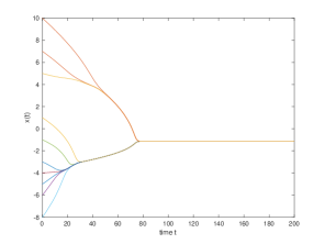
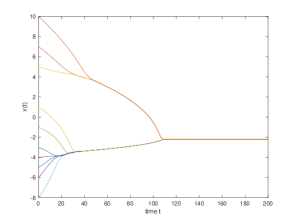
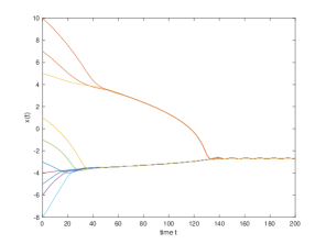
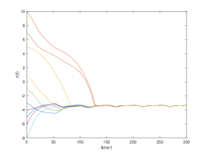
Figure 1: Communication rates (1.3) & $\beta=1$: time evolution of solutions with different strengths of time delays; $\tau=1$ (top left), $\tau=5$ (top right), $\tau=10$ (bottom left), $\tau=50$ (bottom right).

We next take into account short-range interactions compared to the previous case; we chose $\beta=3$ in the weight function $\psi$ in (4.43). In this case, it shows the two clusters formation of solutions as time goes on, not fully consensus behavior, see Figure 2. Note that multi-cluster formation of solutions to the particle system (1.1) with a compactly supported weight function is investigated in [22]. We also provide the time evolution of solutions on the time interval $[0,200]$ or $[0,300]$ in the zoomed images in Figure 2 to take a better look at the oscillatory behavior of solutions depending on the strengths of time delays.

Figure 2: Communication rates (1.3) & $\beta=3$: time evolution of solutions with different strengths of time delays; $\tau=1$ (top left), $\tau=5$ (top right), $\tau=10$ (bottom left), $\tau=50$ (bottom right).

4.2 The particle system (1.1) with (1.4)

In this subsection, we consider the particle system (1.1) with (1.4). Similarly as before, we first investigate the time evolution of solutions for $\beta=1$ in Figure 3. As expected, the consensus behavior of solutions is achieved faster in this case than in the previous case, see also [9, Section 2] for the comparison between the Cucker-Smale flocking model and the Cucker-Smale flocking model with a normalized weight. Compared to the previous case, see Figure 1, it seems that the particle system (1.1) with (1.4) is more sensitive to the strength of time delay; multi-cluster formation is not observed during the time evolution for $\tau=5,10,50$, and after the consensus is achieved, it still highly oscillates, see the case with $\tau=50$ in Figure 3.

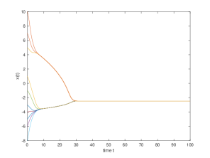
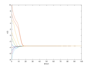
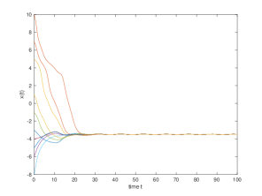
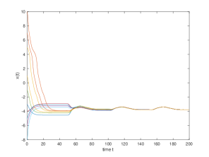
Figure 3: Communication rates (1.4) & $\beta=1$: time evolution of solutions with different strengths of time delays; $\tau=1$ (top left), $\tau=5$ (top right), $\tau=10$ (bottom left), $\tau=50$ (bottom right).

We finally provide the time evolution of solutions for the case $\beta=3$ in Figure 4. Again, in this case, we have the two-cluster formation of solutions. Similarly as before, we put the time evolution of solutions on the time interval $[0,100]$ or $[0,200]$ in the zoomed images in Figure 4 to have a closer look at the oscillatory behavior of solutions with different values of time delays. As mentioned before, we observe the highly oscillatory behavior of solutions as the strength of time delay increases.

Figure 4: Communication rates (1.4) & $\beta=3$: time evolution of solutions with different strengths of time delays; $\tau=1$ (top left), $\tau=5$ (top right), $\tau=10$ (bottom left), $\tau=50$ (bottom right).

References

- [1] A. Aydogdu, M. Caponigro, S. McQuade, B. Piccoli, N. Pouradier Duteil, F. Rossi and E. Trélat. Interaction network, state space and control in social dynamics. Active particles. Vol. 1. Advances in theory, models, and applications, 99–140. Birkhäuser/Springer, Cham, 2017.
- [2] N. Bellomo, M. A. Herrero and A. Tosin, On the dynamics of social conflict: Looking for the Black Swan, Kinet. Relat. Models, 6, (2013), 459–479.
- [3] E. Ben-Naim, Opinion dynamics: rise and fall of political parties, Europhys. Lett., 69, (2005), 671–677.
- [4] F. Bullo, J. Cortés, and S. Martínez. Distributed control of robotic networks: a mathematical approach to motion coordination algorithms. Princeton series in applied mathematics. Princeton University Press, Princeton, 2009.
- [5] S. Camazine, J. L. Deneubourg, N.R. Franks, J. Sneyd, G. Theraulaz and E. Bonabeau, Self-Organization in Biological Systems, Princeton University Press, Princeton, NJ, 2001.
- [6] J. Cañizo, J. Carrillo and J. Rosado, A well-posedness theory in measures for some kinetic models of collective motion, Math. Mod. Meth. Appl. Sci., 21(3), (2011), 515-–539.
- [7] C. Canuto, F. Fagnani and P. Tilli, A Eulerian approach to the analysis of rendez-vous algorithms, IFAC Proceedings Volumes, Vol. 41, (2008), 9039–9044.
- [8] C. Canuto, F. Fagnani and P. Tilli, An Eulerian approach to the analysis of Krause's consensus models, SIAM J. Control Optim., 50, (2012), 243–265.
- [9] J. A. Carrillo, Y.-P. Choi and S. P. Perez A review on attractive-repulsive hydrodynamics for consensus in collective behavior. Active particles. Vol. 1. Advances in theory, models, and applications, 259–298. Birkhäuser/Springer, Cham, 2017.
- [10] J. A. Carrillo, M. Fornasier, G. Toscani and F. Vecil. Mathematical Modeling of Collective Behavior in Socio-Economic and Life Sciences. Chapter Particle, kinetic, and hydrodynamic models of swarming, pages 297–336. Birkhäuser Boston, Boston, 2010.
- [11] C. Castellano, S. Fortunato and V. Loreto, Statistical physics of social dynamics, Rev. Mod. Phys., 81, (2009), 591–646.
- [12] F. Ceragioli and P. Frasca. Continuous and discontinuous opinion dynamics with bounded confidence, Nonlinear Anal. Real World Appl., 13, (2012), 1239–1251.
- [13] Y.-P. Choi and J. Haskovec, Cucker-Smale model with normalized communication weights and time delay, Kinet. Relat. Models, 10, (2017), 1011–1033.
- [14] Y.-P. Choi and Z. Li, Emergent behavior of Cucker-Smale flocking particles with heterogeneous time delays, Appl. Math. Lett., 86, (2018), 49–56.
- [15] Y.-P. Choi and C. Pignotti, Emergent behavior of Cucker-Smale model with normalized weights and distributed time delays, Netw. Heterog. Media, to appear.
- [16] F. Cucker and S. Smale. Emergent behaviour in flocks, IEEE Transactions on Automatic Control, 52, (2007), 852–862.
- [17] J. P. Desai, J. P. Ostrowski, V. Kumar, Modeling and control of formations of nonholonomic mobile robots, IEEE Trans. Robot. Automat., 17, (2001), 905-908.
- [18] B. Düring, P. Markowich, J. F. Pietschmann and M. T. Wolfram, Boltzmann and Fokker–Planck equations modelling opinion formation in the presence of strong leaders, Proc. R. Soc. A, Math. Phys. Eng. Sci., 465, (2009), 3687–3708.
- [19] R. Erban, J. Haskovec and Y. Sun, On Cucker-Smale model with noise and delay, SIAM J. Appl. Math., 76, (2016), 1535–1557.
- [20] J. Haskovec and I. Markou, Delayed Cucker-Smale model with and without noise revisited, Preprint 2018, arXiv:1810.01084.
- [21] R. Hegselmann and U. Krause, Opinion dynamics and bounded confidence models, analysis, and simulation, J. Artif. Soc. Soc. Simul., 5, (2002), 1–24.
- [22] P. E. Jabin and S. Motsch, Clustering and asymptotic behavior in opinion formation, J. Differential Equations, 257, (2014), 4165–4187.
- [23] A. Jadbabaie, J. Lin and A. S. Morse, Coordination of groups of mobile autonomous agents using nearest neighbor rules, IEEE Trans. Automat. Control, 48, (2003), 988-1001.
- [24] J. Lorenz, Continuous opinion dynamics under bounded confidence: a survey, Int. J. Mod. Phys. C, 18, (2007), 1819–1838.
- [25] J. Lu, D. W. C. Ho and J. Kurths, Consensus over directed static networks with arbitrary finite communications delays, Phys. Rev. E, 80, (2009), 066121, 7 pp.
- [26] G. A. Marsan, N. Bellomo and M. Egidi, Towards a mathematical theory of complex socio-economical systems by functional subsystems representation, Kinet. Relat. Models, 1, (2008), 249–278.
- [27] S. Motsch and E. Tadmor. A new model for self–organized dynamics and its flocking behavior, J. Stat. Phys., 144, (2011), 923–947.
- [28] B. Piccoli, N. Pouradier Duteil and E. Trélat, Sparse control of Hegselmann-Krause models: Black hole and declustering, Preprint 2018, ArXiv:1802.00615.
- [29] C. Pignotti and I. Reche Vallejo, Flocking estimates for the Cucker-Smale model with time lag and hierarchical leadership, J. Math. Anal. Appl., 464, (2018), 1313-1332.
- [30] C. Pignotti and E. Trélat, Convergence to consensus of the general finite-dimensional Cucker-Smale model with time-varying delays, Commun. Math. Sci., 16, (2018), 2053–2076.
- [31] S. Y. Pilyugin and M. C. Campi, Opinion formation in voting processes under bounded confidence, Netw. Heterog. Media, 14, (2019), 617–632.
- [32] R. Solé and J. Bascompte, Self-Organization in Complex Eco-systems, Princeton University Press, Princeton, NJ, 2006.
- [33] S. H. Strogatz, C. M. Marcus, R. M. Westervelt and R. E. Mirollo, Simple Model of Collective Transport with Phase Slippage, Phys. Rev. Lett., 61, (1988), 2380–2383.
- [34] S. Wongkaew, M. Caponigro and A. Borzì. On the control through leadership of the Hegselmann-Krause opinion formation model. Math. Models Methods Appl. Sci., 25, (2015), 565–585.
- [35] H. Xu, H. Wang and Z. Xuan, Opinion dynamics: a multidisciplinary review and perspective on future research, Int. J. Knowl. Syst. Sci., 2, (2011), 72–91.