Inter-relations between additive shape invariant superpotentials

Abstract

All known additive shape invariant superpotentials in nonrelativistic quantum mechanics belong to one of two categories: superpotentials that do not explicitly depend on $\hbar$, and their $\hbar$-dependent extensions. The former group themselves into two disjoint classes, depending on whether the corresponding Schrödinger equation can be reduced to a hypergeometric equation (type-I) or a confluent hypergeometric equation (type-II). All the superpotentials within each class are connected via point canonical transformations. Previous work Gangopadhyaya showed that type-I superpotentials produce type-II via limiting procedures. In this paper we develop a method to generate a type I superpotential from type II, thus providing a pathway to interconnect all known additive shape invariant superpotentials.

I Introduction and Background

I.1 Supersymmetric Quantum Mechanics

Supersymmetric quantum mechanics (SUSYQM) is a generalization of the Dirac-Föck ladder method for the harmonic oscillator Witten ; Solomonson ; CooperFreedman . In SUSYQM, a general hamiltonian $H_{-}$ is written in terms of ladder-operators ${\cal A}^{+}\equiv-\frac{\hbar}{\sqrt{2m}}\frac{d}{dx}+W(x,a)$ and ${\cal A}^{-}\equiv\frac{\hbar}{\sqrt{2m}}\frac{d}{dx}+W(x,a)$, where the function $W(x,a)$, a real function of $x$ and a parameter $a$, is known as the superpotential. Henceforth, we set $2m=1$. The hamiltonian $H_{-}$ is given by

$$H_{-}={\cal A}^{+}\,{\cal A}^{-} = \left(-\hbar\frac{d}{dx}+W(x,a)\right)~{}\left(\hbar\frac{d}{dx}+W(x,a)\right)$$ (1)

$$= -\hbar^{2}\frac{d^{2}}{dx^{2}}+W^{2}(x,a)-\hbar\,\frac{dW(x,a)}{dx}~{}$$

$$= -\hbar^{2}\frac{d^{2}}{dx^{2}}+V_{-}(x,a),$$

where $V_{-}(x,a)=W^{2}(x,a)-\hbar~{}{dW}/{dx}$. The product of operators ${\cal A}^{-}{\cal A}^{+}$ generates another hamiltonian $H_{+}=-\hbar^{2}\frac{d^{2}}{dx^{2}}+V_{+}(x,a)$ with $V_{+}(x,a)=W^{2}(x,a)+\hbar~{}{d\,W}/{dx}$. These two hamiltonians are related by ${\cal A}^{+}H_{+}=H_{-}\,{\cal A}^{+}$ and ${\cal A}^{-}H_{-}=H_{+}\,{\cal A}^{-}$, which leads to the following isospectrality relationships among their eigenvalues and eigenfunctions for all integer $n\geq 0$:

$$E^{-}_{n+1}=E^{+}_{n};\qquad\frac{~{}~{}~{}{\cal A}^{-}}{\sqrt{E^{+}_{n}}}~{}\psi^{(-)}_{n+1}=~{}\psi^{(+)}_{n}\,,~{}~{}{\rm and}\quad\frac{~{}~{}~{}{\cal A}^{+}}{\sqrt{E^{+}_{n}}}~{}\psi^{(+)}_{n}=~{}\psi^{(-)}_{n+1}.$$ (2)

Thus, if we knew the eigenvalues and eigenstates of the hamiltonian $H_{-}$, we would automatically know the same for the hamiltonian $H_{+}$, and vice-versa. For unbroken SUSY, if a superpotential $W(x,a_{i})$ obeys a particular constraint known as “shape invariance”, then the eigenvalues and eigenfunctions for both hamiltonians can be determined separately. In this manuscript, we will consider only unbroken SUSY.

I.2 Shape Invariance

Let us consider a set of parameters $a_{i}$, $i=0,1,2,\cdots$, with $a_{0}=a$, and $a_{i+1}=f(a_{i})$, where $f$ is a function of $a_{i}$. A superpotential $W(x,a_{i})$ is shape invariant if it obeys the following condition Infeld ; Miller ; Gendenshtein1 ; Gendenshtein2 :

$$W^{2}(x,a_{i})+\hbar\,\frac{d\,W(x,a_{i})}{dx}+g(a_{i})=W^{2}(x,a_{i+1})-\hbar\,\frac{d\,W(x,a_{i+1})}{dx}+g(a_{i+1}).~{}$$ (3)

The eigenvalues and eigenfunctions are given by Cooper-Khare-Sukhatme ; Gangopadhyaya-Mallow-Rasinariu

$$E_{n}^{(-)}(a_{0})=g(a_{n})-g(a_{0})~{}~{}{\rm for}~{}n\geq 0~{},$$

and

$$\psi^{(-)}_{n}(x,a_{0})\sim{\cal A}^{+}{(a_{0})}~{}{\cal A}^{+}{(a_{1})}\cdots{\cal A}^{+}{(a_{n-1})}~{}\psi^{(-)}_{0}(x,a_{n})~{},$$

where $\psi^{(-)}_{0}(x,a_{n})\sim\exp\left\{-\frac{1}{\hbar}\,\int^{x}W(y,a_{n})\,dy\right\}$. This solvability of all additive shape invariant systems, which stems from Eq. (3), can be related to underlying potential algebras of the systems Gangopadhyaya_algebra1 ; Balantekin1 ; Gangopadhyaya_algebra2 ; Gangopadhyaya_algebra3 ; Balantekin2 .

Hereafter, we consider the case of translational or additive shape invariance: $a_{i+1}=a_{i}+\hbar$.

II Shape Invariant Superpotentials

Shape invariant systems are of great importance in quantum mechanics due to their exact solvability; hence, it is desirable to determine as many shape invariant superpotentials (SISs) as possible. All SISs obey Eq. (3), which is a non-linear difference-differential equation. Several investigators have found solutions to this equation Infeld ; Gendenshtein1 ; Dutt ; CGK . The authors of Ref. Gangopadhyaya_NPDE ; Bougie2010 ; symmetry reduced Eq. (3) to two local partial differential equations (PDEs) and proved that the list of SISs listed in Infeld ; Gendenshtein1 ; Dutt ; CGK is complete, under the assumption that $W(x,a)$ does not depend explicitly on $\hbar$. The set of superpotentials generated by solving the two PDEs was called “conventional”.

In 2008, two additional shape invariant superpotentials were discovered Quesne1 ; Quesne2 that were not included in previous lists of conventional superpotentials. These superpotentials were then generalized in Ref.Odake1 ; Odake2 ; Tanaka ; Odake3 ; Odake4 ; Quesne2012a ; Quesne2012b , and some of their properties have been further studied Ranjani1 ; Ramos2011 . Since these superpotentials could not be generated from the two PDEs, they must contain explicit $\hbar$-dependence. In Ref. Bougie2010 ; symmetry , the authors showed that these superpotentials obey an infinite set of PDEs. In this section, we will describe how to generate these shape invariant systems from the PDEs.

II.1 Conventional Superpotentials

We begin with conventional superpotentials, for which $W(x,a_{i})$ has no explicit dependence on $\hbar$; i.e., any dependence on $\hbar$ enters only through the linear combination $a_{i+1}=a_{i}+\hbar$. Since Eq. (3) must hold for an arbitrary value of $\hbar$, we can expand the equation in powers of $\hbar$, and require that the coefficient of each power vanishes, leading to the following two independent equations Bougie2010 ; symmetry :

$$\vspace{6pt}W\,\frac{\partial W}{\partial a}-\frac{\partial W}{\partial x}+\frac{1}{2}\,\frac{dg(a)}{da}=0~{}$$ (4)

and

$$\frac{\partial^{3}}{\partial a^{2}\partial x}~{}W(x,a)=0~{}.$$ (5)

The general solution to Eq. (5) is

$$W(x,a)=a\cdot\chi_{1}(x)+\chi_{2}(x)+u(a)~{}.$$ (6)

When combined with Eq. (4), this solution reproduces the complete family of conventional superpotentials, as shown in Table (1) Bougie2010 ; symmetry .

These conventional superpotentials generate special cases of the Natanzon potentials Natanzon ; Cooper-Khare-Sukhatme ; Gangopadhyaya-Mallow-Rasinariu . They fall into one of two categories, depending on whether the corresponding Schrödinger equation can be reduced to a hypergeometric equation (type-I) or a confluent hypergeometric equation (type-II) DeDuttSukhatme ; Gangopadhyaya .

	Name	Superpotential	Type
1	Scarf (Hyperbolic)	$A\tanh x+B\,{\rm sech}\,x$	I
2	Gen. Pöschl-Teller	$A\coth r-B\,{\rm cosech}\,r$	I
3	Scarf (Trigonometric)	$A\tan x-B\,{\rm sec}\,x$	I
4	Rosen-Morse I	$-A\cot x-\frac{B}{A}$	I
5	Rosen-Morse II	$A\tanh x+\frac{B}{A}$	I
6	Eckart	$-A\coth r+\frac{B}{A}$	I
a	Morse	$A-B\,e^{-x}$	II
b	3-D oscillator	$\frac{1}{2}\omega r-\frac{\ell}{r}$	II
c	Coulomb	$\frac{e^{2}}{2\ell}-\frac{\ell}{r}$	II
d	Harmonic Oscillator	$\frac{1}{2}\omega x$	II

Table 1: The complete family of $\hbar$-independent additive shape-invariant superpotentials.

II.2 Extended Superpotentials

Table (1) lists the exhaustive set of superpotentials that are $\hbar$-independent. However, this list does not include the $\hbar$-dependent shape invariant superpotentials reported in Quesne1 ; Quesne2 , or their generalizations Odake1 ; Odake2 ; Tanaka ; Odake3 ; Odake4 . All known $\hbar$-dependent superpotentials can be written as $W(x,a,\hbar)=W_{0}(x,a)+W_{h}(a,x,\hbar)$, where the kernel $W_{0}$ is one of the conventional superpotentials listed in Table 1, and $W_{h}$ is an explicitly $\hbar$-dependent extension of that kernel. For example, one superpotential found in Quesne1 can be written as

$$W(r,\ell,\hbar)=\frac{1}{2}\,\omega r-\frac{\ell}{r}+\left(\frac{2\omega r\hbar}{\omega r^{2}+2\ell-\hbar}-\frac{2\omega r\hbar}{\omega r^{2}+2\ell+\hbar}\right)~{},$$ (7)

where $W_{0}=\frac{1}{2}\,\omega r-\frac{\ell}{r}$ is the conventional superpotential of the 3-D oscillator, and the term in parenthesis is $W_{h}$, the $\hbar$-dependent extension.

Because extended superpotentials depend explicitly on $\hbar$, we can expand them in powers of $\hbar$:

$$\vspace{6pt}W(x,a,\hbar)=\sum_{j=0}^{\infty}\hbar^{j}W_{j}(x,a).~{}$$ (8)

Since $a_{0}=a$ and $a_{1}=a+\hbar$, we also have

$$W\left(x,a_{1},\hbar\right)=\sum_{j=0}^{\infty}\sum_{k=0}^{j}\frac{\hbar^{j}}{k!}\frac{\partial^{k}W_{j-k}}{\partial a^{k}},$$

which we then substitute back into Eq. (3). Since Eq. (3) must hold for any value of $\hbar$, we set the coefficients of the series for each power of $\hbar$ equal to zero. This gives, for $j=1$

$$2\frac{\partial W_{0}}{\partial x}-\frac{\partial}{\partial a}\left(W_{0}^{2}+g\right)=0,$$ (9)

and for $j\geq 2$

$$2\,\frac{\partial W_{j-1}}{\partial x}-\sum_{s=1}^{j-1}\sum_{k=0}^{s}\frac{1}{(j-s)!}\frac{\partial^{j-s}}{\partial a^{j-s}}W_{k}\,W_{s-k}+\sum_{k=2}^{j-1}\frac{1}{(k-1)!}\frac{\partial^{k}\,W_{j-k}}{\partial a^{k-1}\,\partial x}=0~{}.$$ (10)

In Refs. Bougie2010 and symmetry the authors explicitly generated the extended superpotential (7) from these partial differential equations.

III Known Relationships Between Shape-Invariant Superpotentials

In this section we discuss the known connections between SISs. They are: point canonical transformations, projections, and isospectral extensions.

III.1 Point Canonical Transformations

We begin with the relationships between the various conventional superpotentials that are connected via point canonical transformations (PCTs). A PCT comprises a change of the independent variable $x$ and an associated multiplicative transformation of the wavefunction in a Schrödinger equation, such that it generates a new Schrödinger equation Bhattacharjie ; DeDuttSukhatme .

For a change of variable from $x\to z$, where $x=u(z)$ and a corresponding change in wave function that relates the new wave function $\tilde{\psi}$ to the old by $\psi(x)=\tilde{\psi}(z)\,\sqrt{du/dz}$, the Schrödinger equation

$$-\frac{d^{2}\psi(x)}{dx^{2}}+V(x,a_{i})\,\psi(x)=E(a_{i})\psi(x)$$ (11)

transforms into:

$$\left[-\frac{d^{2}}{dz^{2}}+\left\{\dot{u}^{\,2}\,\left[V(u(z),a_{i})-E(a_{i})\right]+{\frac{1}{2}}\left(\frac{3\ddot{u}^{\,2}}{2\dot{u}^{\,2}}-\frac{\dddot{u}}{\dot{u}}\right)\right\}\right]\tilde{\psi}\left(z\right)=0.$$ (12)

where $\dot{u}=du/dz$, etc. For Eq. (12) to be a Schrödinger equation, an energy term must emerge from the expression $\dot{u}^{\,2}\,\left[V(u(z),a_{i})-E(a_{i})\right]$; i.e., it must have a term that is independent of $z$. This condition constrains the choices for the function $u(z)$.

The six type-I superpotentials are characterized by corresponding Schrödinger equations that can be transformed into a hypergeometric equation. If we consider the one-dimensional harmonic oscillator to be a simplified case of the 3-D oscillator ($\ell=0$) , we have three type-II superpotentials, which correspond to the confluent hypergeometric equation. Each type-I superpotential can be mapped to each other type-I superpotential via PCTs, and each type-II superpotential can be similarly mapped to each other type-II superpotential CooperGinocchioWipf ; DeDuttSukhatme ; Levai . The corresponding PCTs, illustrated in Figure 1, are given by $T_{12}\!:\!\{x\to r+i\pi/2\},\,T_{23}\!:\!\{r\to ix+i\pi/2\},\,T_{34}\!:\!\{x\to\cos^{-1}(\text{cosec }x)\},\,T_{45}\!:\!\{x\to\pi/2+ix\},\,T_{56}\!:\!\{x\to-r+i\pi/2\},\,T_{61}\!:\!\{r\to\coth^{-1}(i\sinh x)\},\,T_{ab}\!:\!\{x\to-2\ln r\},\,T_{bc}\!:\!\{r\to\sqrt{z}\},\,$ and $T_{ca}\!:\!\{r\to\exp(-x)\}\,.$

III.2 Projections

PCTs cannot transform type-I to type-II or vice-versa. The hypergeometric differential equation, corresponding to type-I superpotentials, has three regular singular points. With suitable limits, two of the singularities merge, and the equation reduces to a confluent hypergeometric equation, connected to the type-II superpotential. Thus, these limiting procedures generate “projections” from type-I to type-II superpotentials, making it possible to move from one type to another, albeit in only one direction, as shown in Table 2, and in Figure 1.

Type-I Superpotential	Projection	Type-II Superpotential
1) Scarf (Hyperbolic)	$P_{1a}:$	a) Morse
$W(x)=A\tanh\left(x+\beta\right)+B~{}\textrm{sech}\left(x+\beta\right)$	$A\to A$	$W(x)=A-B\,e^{-x}$
$-\infty<x<\infty,\;A>0$	$B\to-B\,{e^{\beta}\over 2}$	$-\infty<x<\infty$
$E_{n}=A^{2}-\left(A-n\hbar\right)^{2}$	$\beta\to\infty$	$E_{n}=A^{2}-\left(A-n\hbar\right)^{2}$
2) Generalized Pöschl-Teller	$P_{2a}$:	a) Morse
$W(r)=A\coth\left(\alpha r+\beta\right)-B~{}\textrm{cosech}\,\left(\alpha r+\beta\right)$	$A\to A$	$W(x)=A-B\,e^{-x}$
	$B\to B\,{e^{\beta}\over 2}$, $\alpha\to 1$	$-\infty<x<\infty$
	$\beta\to\infty$, $r\to x$	$E_{n}=A^{2}-\left(A-n\hbar\right)^{2}$
	$P_{2b}:$	b) 3-D Oscillator
$-\frac{\beta}{\alpha}<r<\infty$	$A\to\left({\omega\over\alpha}-\frac{\alpha\ell}{2}\right)$	$W(r)=\frac{1}{2}\omega r-\frac{\ell}{r}$
$E_{n}=A^{2}-\left(A-n\alpha\hbar\right)^{2}$	$B\to\left({\omega\over\alpha}+\frac{\alpha\ell}{2}\right)$	$0<r<\infty$
$A<B$	$\beta\to 0$, $\alpha\to 0$	$E_{n}=2n\omega\hbar$
3) Scarf (Trigonometric)	$P_{3b}:$	b) 3-D Oscillator
$W(x)=A\tan\left(\alpha x\right)-B\sec\left(\alpha x\right)$	$A\to\left({\omega\over\alpha}+\frac{\alpha\ell}{2}\right)$	$W(r)=\frac{1}{2}\omega r-\frac{\ell}{r}$
$-{\pi\over 2\alpha}<x<{\pi\over 2\alpha},~{}A>B$	$B\to\left({\omega\over\alpha}-\frac{\alpha\ell}{2}\right)$	$0<r<\infty$
$E_{n}=\left(A+n\alpha\hbar\right)^{2}-A^{2}$	$x\to r+{\pi\over 2\alpha}$, $\alpha\to 0\;$	$E_{n}=2n\omega\hbar$
4) Rosen-Morse I	$P_{4c}:$	c) Coulomb
$W(x)=-A\cot\left(\alpha x\right)-\frac{B}{A}$	$A\to\alpha\ell$	$W(r)=\frac{e^{2}}{2\ell}-\frac{\ell}{r}$
$0<x<\frac{\pi}{\alpha}$	$B\to-{\alpha\over 2}e^{2}$	$0<r<\infty$
$E_{n}=-A^{2}+\left(A+n\alpha\hbar\right)^{2}+{B^{2}\over A^{2}}-{B^{2}\over{(A+n\alpha\hbar)}^{2}}$	$\alpha\to 0$, $x\to r$	$E_{n}={e^{4}\over{4\hbar^{2}}}\left({1\over l^{2}}-{1\over(n+l)^{2}}\right)$
5) Rosen-Morse II	—	—
$W(x)=A\tanh(x)+\frac{B}{A}$
$-\infty<x<\infty$, $B<A^{2}$
$E_{n}=A^{2}-\left(A-n\hbar\right)^{2}-\frac{B^{2}}{(A-n\hbar)^{2}}+\frac{B^{2}}{A^{2}}$
6) Eckart	$P_{6c}:$	c) Coulomb
$W(r)=-A\rm{coth}\left(\alpha r\right)+\frac{B}{A}$	$A\to\alpha\ell$	$W(r)=\frac{e^{2}}{2\ell}-\frac{\ell}{r}$
$0<r<\infty,\;B>A^{2},\;A>0$	$B\to{\alpha\over 2}e^{2}$	$0<r<\infty$
$E_{n}=A^{2}-\left(A+n\alpha\hbar\right)^{2}+{B^{2}\over A^{2}}-{B^{2}\over{(A+n\alpha\hbar)}^{2}}$	$\alpha\to 0$	$E_{n}={e^{4}\over{4\hbar^{2}}}\left({1\over l^{2}}-{1\over(n+l)^{2}}\right)$

Table 2: Limiting procedures and redefinition of parameters relating type-I to type-II superpotentials. For projections, in each cell the order of operators should be carried out from top to bottom.

III.3 Isospectral Extensions

For extended superpotentials, the energy spectrum is given entirely by the $\hbar-$independent kernel $W_{0}$ symmetry , and every known $\hbar-$dependent SIS contains a conventional SIS as its kernel. These extended superpotentials can therefore be obtained from conventional superpotentials through an isospectral process that adds an $\hbar$-dependent term to the conventional superpotential while maintaining shape-invariance. In the limit $\hbar\to 0$, each reduces to its corresponding conventional counterpart.

IV Generating a Pathway from Type-II to Type-I Superpotentials

We have seen that the six SISs of type-I are interconnected via PCTs; so are the three type-II SISs. Furthermore, type-I SISs reduce to type-II via projections. Graphically, these interrelations are illustrated in Figure 1.

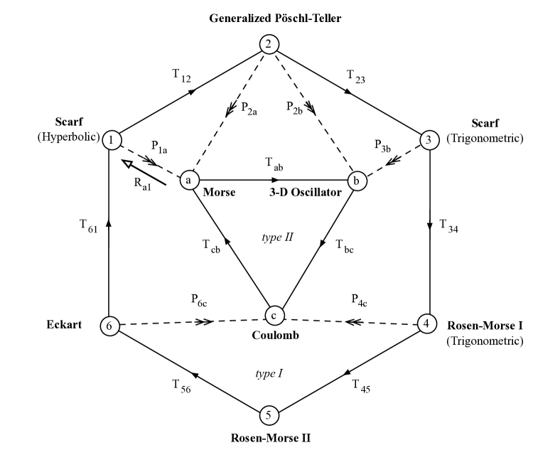
Figure 1: Inter-relations among conventional superpotentials. PCTs are represented by plain lines with arrows while the projections from type-I to type-II are represented by dashed lines with double arrows; the projection corresponding to each label is given in Table 2. $R_{a1}$ will be discussed below.

Additionally, the extended SISs are obtained from conventional SISs by isospectral extension and they reduce to the conventional ones when $\hbar\to 0$.

However, we have no connection yet that will take us from a type-II to a type-I superpotential. So far, the connections between the SISs have been of three types: (i) PCTs, (ii) projections, and (iii) isospectral extensions. We now ask whether we can employ any of these three mechanisms to go from type-II to type-I.

Of these three mechanisms, PCTs map superpotentials within a given type (I or II), but do not move between types. Projections reduce the hypergeometric equation to the confluent hypergeometric equation, but do not do the reverse. This leaves the isospectral extension, which allows for the addition of terms to an initial kernel $W_{0}$. We choose this kernel to be Morse, because it is the only type-II SIS that is isospectral with type-I SISs. Therefore, if such a reverse path, denoted $R_{a1}$ in Figure 1, exists, then it should start from Morse.

We proceed to construct an extension using Eq. (10). In Ref. Quesne2012b , the author generated a quasi-exactly solvable extension of Morse and showed that it was not shape invariant. The strength of the isospectral extension method is that we can employ Eq. (10) term-by-term in order to generate a manifestly shape-invariant solution. The Morse superpotential is

$$W_{0}=-a-e^{-x}~{},$$

where, without loss of generality, we set $a\equiv-A<0$, and $B=1$. Choosing $W_{1}=0$, the equation for $W_{2}$ reads

$$\frac{\partial W_{2}}{\partial x}-\frac{\partial W_{0}W_{2}}{\partial a}=0~{}.$$

A solution is

$$W_{2}(x,a)=e^{-x}\left(2P+Qe^{-2x}+2a~{}Qe^{-x}\right)~{},$$

where $P$ and $Q$ are constant parameters. Choosing $W_{3}$ to be zero, the equation for $W_{4}$ is

$$2\frac{\partial W_{4}}{\partial x}-2\frac{\partial\left(W_{0}W_{4}+\frac{1}{2}W_{2}^{2}\right)}{\partial a}-\frac{\partial}{\partial a}\left(\frac{\partial W_{2}}{\partial a}\frac{\partial W_{0}}{\partial a}\right)$$

$$-\frac{1}{3}\left(W_{2}\frac{\partial^{3}W_{0}}{\partial a^{3}}+W_{0}\frac{\partial^{3}W_{2}}{\partial a^{3}}\right)+\frac{1}{2}\frac{\partial^{3}W_{2}}{\partial x\partial a^{2}}=0$$

The above equation is solved by

$$W_{4}(x,a)=-Qe^{-3x}\left(2P+Qe^{-2x}+2a~{}Qe^{-x}\right)~{}.$$

Generalizing this process yields $W_{2k-1}=0$ and

$$W_{2k}=\left(-Q\right)^{k-1}e^{-(2k-1)x}\left(2P+Qe^{-2x}+2a~{}Qe^{-x}\right)$$

for all positive integers $k.$ Computing the infinite sum $\sum_{j=0}^{\infty}\hbar^{j}W_{j}(x,a)$, we obtain

$$W(x,a,\hbar)=-a-e^{-x}+\frac{\hbar^{2}\left(2Pe^{x}+2a\,Q+Q\,e^{-x}\right)}{e^{2x}+Q\,\hbar^{2}}~{}.$$ (13)

The shape invariance of this superpotential can be directly checked. Substituting the above expression into Eq. (3) yields

$$W^{2}(x,a)-W^{2}(x,a+\hbar)+\hbar\frac{d\,}{dx}\left(W(x,a)+W(x,a+\hbar)\right)=-\hbar(2a+\hbar),$$ (14)

which can be brought into the form of Eq. (3) by choosing $g(a)=-a^{2}$. This leads to the energy eigenvalues $E^{(-)}_{n}=g(a+n\hbar)-g(a)=a^{2}-(a+n\hbar)^{2}$. As expected, these values are the same as those of the Morse potential. Note that as $\hbar\to 0$, we recover the starting kernel, which is the Morse superpotential.

The superpotential Eq. (13) was initially reported in Ref.Bougie2015 as a new $\hbar$-dependent extension of the Morse superpotential. However, here we show that it is in fact equivalent to the conventional Scarf hyperbolic superpotential. To do so, we absorb $\hbar$ in Eq. (13) into another set of parameters via the following transformations:

$$\hbar^{2}P\to P^{\,\prime},~{}\hbar^{2}Q\to e^{2\beta},~{}(2P^{\,\prime}-1)\,e^{-\beta}\to 2B,~{}-a\to A,~{}x-\beta\to x~{}.$$ (15)

These transformations effectively map the “extended” superpotential (13) into the Scarf hyperbolic, a conventional type-I superpotential   :

$$-a-e^{-x}+\frac{\hbar^{2}\left(2P\,e^{x}+2a\,Q+Q\,e^{-x}\right)}{e^{2x}+Q\,\hbar^{2}}~{}\to W_{Scar\!f}=A\tanh x+B\,\textrm{sech}\,x~{}.$$ (16)

Thus, in this case, rather than producing a new superpotential, this technique created a “restricted extension” $R_{a1}$, from a type-II to a type-I superpotential. $R_{a1}$ was the missing link in the quest to provide a connection between all known additive shape invariant superpotentials. Now, we have a bidirectional way to connect any pair of known additive shape-invariant superpotentials, via a combination of PCTs, projections, and isospectral extensions.

V Conclusions

In this manuscript, we have shown via an explicit construction that the Morse superpotential can be isospectrally deformed via the extension mechanism into the Scarf hypergeometric superpotential. As a result, we have demonstrated that there exists a path from a type-II to a type-I superpotential; thus, all known additive shape-invariant superpotentials are inter-related through a combination of PCTs, projections, and isospectral extensions.

References

- (1) A. Balantekin, M. Candido Ribeiro, and A. Aleixo. Algebraic Nature of Shape-Invariant and Self-Similar Potentials. J. Phys. A, 32:2785 – 2790, 1999.
- (2) A. B. Balantekin. Algebraic Approach to Shape Invariance. Phys. Rev. A, 57:4188 – 4191, 1998.
- (3) A. Bhattacharjie and E.C.G. Sudarshan. A Class of Solvable Potentials. Nuovo Cimento, 25:864–879, 1962.
- (4) J. Bougie, A. Gangopadhyaya, and J. V. Mallow. Generation of a Complete Set of Additive Shape-Invariant Potentials From an Euler Equation. Phys. Rev. Lett., 105:210402, 2010.
- (5) J. Bougie, A. Gangopadhyaya, J. V. Mallow, and C. Rasinariu. Supersymmetric Quantum Mechanics and Solvable Models. Symmetry, 4:452–473, 2012.
- (6) J. Bougie, A. Gangopadhyaya, J. V. Mallow, and C. Rasinariu. Generation of a Novel Exactly Solvable Potential. Physics Letters A, 379(37):2180 – 2183, 2015.
- (7) José F. Cariñena and Arturo Ramos. Riccati equation, factorization method and shape invariance. Reviews in Mathematical Physics, 12(10):1279–1304, 2000.
- (8) S. Chaturvedi, R. Dutt, A. Gangopadhyaya, P. Panigrahi, C. Rasinariu, and U. Sukhatme. Algebraic Shape Invariant Models. Phys. Lett., A248:109 – 113, 1998.
- (9) F. Cooper and B. Freedman. Aspects of Supersymmetric Quantum Mechanics. Ann. Phys., 146:262–288, 1983.
- (10) F. Cooper, J. N. Ginocchio, and A. Khare. Relationship Between Supersymmetry and Solvable Potentials. Phys. Rev. D, 36:2458–2473, 1987.
- (11) F. Cooper, J. N. Ginocchio, and A. Wipf. Supersymmetry, Operator Transformations and Exactly Solvable Potentials. A. Math. Gen., 22:3707 – 3716, 1989.
- (12) F. Cooper, A. Khare, and U. Sukhatme. Supersymmetry in Quantum Mechanics. World Scientific, Singapore, 2001.
- (13) R. De, R. Dutt, and U. Sukhatme. Mapping of Shape Invariant Potentials Under Point Canonical Transformations. J. Phys A. Math. Gen., 22:L843, 1992.
- (14) R. Dutt, A. Khare, and U. Sukhatme. Exactness of Supersymmetry WKB Spectra for Shape-Invariant Potentials. Phys. Lett. B, 181:295–298, 1986.
- (15) A. Gangopadhyaya, J. Mallow, and C. Rasinariu. Supersymmetric Quantum Mechanics: An Introduction. World Scientific, Singapore, 2017.
- (16) A. Gangopadhyaya and J. V. Mallow. Generating Shape Invariant Potentials. Int. J. Mod. Phys. A, 23:4959 – 4978, 2008.
- (17) A. Gangopadhyaya, J. V. Mallow, and U. P. Sukhatme. Shape invariance and its connection to potential algebra. In H. Aratyn, T. D. Imbo, W.-Y. Keung, and U. Sukhatme, editors, Supersymmetry and Integrable Models: Proceedings of Workshop on Supersymmetry and Integrable Models. Springer-Verlag: Berlin, Germany, 1997.
- (18) A. Gangopadhyaya, J. V. Mallow, and U. P. Sukhatme. Translational Shape Invariance and the Inherent Potential Algebra. Phys. Rev. A, 58:4287 – 4292, 1998.
- (19) A. Gangopadhyaya, P.K. Panigrahi, and U. P. Sukhatme. Inter-Relations of Solvable Potentials. Helv. Phys. Acta, 67:363 – 368, 1994.
- (20) L. E. Gendenshtein. Derivation of Exact Spectra of the Schrödinger Equation by Means of Supersymmetry. JETP Lett., 38:356–359, 1983.
- (21) L. E. Gendenshtein and I. V. Krive. Supersymmetry in Quantum Mechanics. Sov. Phys. Usp., 28:645–666, 1985.
- (22) L. Infeld and T. E. Hull. The Factorization Method. Rev. Mod. Phys., 23:21–68, 1951.
- (23) G. Lévai. Solvable Potentials Derived from Supersymmetric Quantum Mechanics. In H. V. von Geramb, editor, Quantum Inversion Theory and Applications, pages 107–126, Berlin, Heidelberg, 1994. Springer Berlin Heidelberg.
- (24) W. Miller. Lie Theory and Special Functions. Academic Press, New York, 1968.
- (25) G. A. Nathanzon. Study of the one-dimensional schroödinger equation generated from the hypergeometric equation. Vestnik Leningradskoyo Universiteta, pages 22–28, 1971.
- (26) S. Odake and R. Sasaki. Infinitely Many Shape Invariant Discrete Quantum Mechanical Systems and New Exceptional Orthogonal Polynomials Related to the Wilson and Askey-Wilson Polynomials. Phys. Lett. B, 682:130–136, 2009.
- (27) S. Odake and R. Sasaki. Another Set of Infinitely Many Exceptional Laguerre Polynomials. Phys. Lett. B, 684:173–176, 2010.
- (28) S. Odake and R. Sasaki. Exactly Solvable Quantum Mechanics and Infinite Families of Multi-Indexed Orthogonal Polynomials. Phys. Lett. B, 702:164–170, 2011.
- (29) S. Odake and R. Sasaki. Extensions of Solvable Potentials with Finitely Many Discrete Eigenstates. J. Phys. A, 46:235205, 2013.
- (30) C. Quesne. Exceptional Orthogonal Polynomials, Exactly Solvable Potentials and Supersymmetry. J. Phys. A, 41:392001, 2008.
- (31) C. Quesne. Solvable Rational Potentials and Exceptional Orthogonal Polynomials in Supersymmetric Quantum Mechanics. Sigma, 5:084, 2009.
- (32) C. Quesne. Novel Enlarged Shape Invariance Property and Exactly Solvable Rational Extensions of the Rosen-Morse II and Eckart Potentials. Sigma, 8:080, 2012.
- (33) C. Quesne. Revisiting (Quasi-)Exactly Solvable Rational Extensions of the Morse Potential. Int. J. Mod. Phys. A, 27:1250073, 2012.
- (34) Arturo Ramos. On the new translational shape-invariant potentials. Journal of Physics A: Mathematical and Theoretical, 44(34):342001, aug 2011.
- (35) S. S. Ranjani, P. K. Panigrahi, A. K. Kapoor, A. Khare, and A. Gangopadhyaya. Exceptional Orthogonal Polynomials, QHJ Formalism and SWKB Quantization. J. Phys. A, 45:055210, 2012.
- (36) P. Solomonson and J. W. Van Holten. Fermionic Coordinates and Supersymmetry in Quantum Mechanics. Nucl. Phys. B, 196:509–531, 1982.
- (37) T. Tanaka. N-Fold Supersymmetry and Quasi-Solvability Associated With X-2-Laguerre Polynomials. J. Math. Phys., 51:032101, 2010.
- (38) E. Witten. Dynamical Breaking of Supersymmetry. Nucl. Phys. B, 185:513–554, 1981.