Coupled $K^{+}\Lambda$ and $K^{0}\Lambda$ photoproduction off the nucleon: Consequences from the recent CLAS and MAMI data and the $N(1680)P_{11}$ narrow state

Abstract

The new $\gamma n\to K^{0}\Lambda$ data obtained from the CLAS and MAMI collaborations are analyzed by employing an effective Lagrangian method. The constructed model can describe all available experimental data in both $\gamma p\to K^{+}\Lambda$ and $\gamma n\to K^{0}\Lambda$ channels, simultaneously. The background part of the model is built from the appropriate intermediate states involving the nucleon, kaon, and hyperon exchanges, whereas the resonance part is constructed from the consistent interaction Lagrangians and propagators. To check the performance of the model a detailed comparison between the calculated observables and experimental data in both isospin channels is presented, from which a nice agreement can be observed. The discrepancy between the CLAS and MAMI data in the $\gamma n\to K^{0}\Lambda$ channel is analyzed by utilizing three different models; M1, M2, and M3 that fit the CLAS, MAMI, and both CLAS and MAMI data sets, respectively. The effect of this discrepancy is studied by investigating the significance of individual nucleon resonances and the predicted beam-target helicity asymmetry $E$ that has been measured by the CLAS collaboration recently. It is found that the $N(1720)P_{13}$, $N(1900)P_{13}$, and $N(2060)D_{15}$ resonances are significant for improving the agreement between model calculation and data. This result is relatively stable to the choice of the model. The helicity asymmetry $E$ can be better explained by the models M1 and M3. Finally, the effect of the $N(1680)P_{11}$ narrow resonance on the cross section of both isospin channels is explored. It is found that the effect is more sensitive in the $\gamma n\to K^{0}\Lambda$ channel. In this case the model M3, that fits both CLAS and MAMI data, yields a more realistic effect.

I INTRODUCTION

Among the six possible isospin channels in kaon photoproduction, the $\gamma p\to K^{+}\Lambda$ channel is the first channel and most studied channel during the last six decades. This is understandable because from both theoretical and experimental points of view this channel is the simplest, although accurate data could only be obtained in the last two decades after the use of continuous and heavy duty accelerators along with the unprecedented precise detectors. As a consequence, the $K^{+}\Lambda$ channel has the largest experimental database collected from different measurements performed in the modern accelerator facilities, such as CEBAF in Jefferson Lab, SPring8 in Osaka, MAMI in Mainz, ELSA in Bonn and ESRF in Grenoble. These accurate data allow for detailed analyses of certain nucleon and delta resonances in kaon photoproduction that are not available in other meson photoproductions due to their large kaon branching ratios. Further information to this end can be found, e.g., in our recent reports Mart:2017mwj ; Clymton:2017nvp .

The history of kaon photoproduction presumably started with the theoretical analysis by Kawaguchi and Moravcsik more than 60 years ago masasaki , after the work of Chew, Goldberger, Low, and Nambu (known later as the CGLN amplitude) chew . In their analysis, Kawaguchi and Moravcsik considered all six possible isospin channels by using only three Feynman diagrams of the Born terms, in spite of the fact that no experimental data were available at that time. Furthermore, the parities of the $\Lambda$ and $\Sigma^{0}$ hyperons were also not known, although they decisively control the cross section magnitude. Therefore, it is safe to consider the pioneering work of Thom in 1966 thom as a more serious attempt to this end, since both Born and resonance terms had been considered, while coupling constants in the Born term and some resonance parameters in the resonance term were fitted to 58 experimental data points (46 points of differential cross sections and 12 points of $\Lambda$ polarization).

The interest in the kaon photoproduction temporarily declined after the midseventies, particularly due to the lack of new experimental data. However, with the construction of new generation of high duty-factor accelerators that provide continuous, high current, and polarized photon beams in the energy regime of a few GeV in Mainz (MAMI), Bonn (ELSA), Newport News (CEBAF), Grenoble (ESRF), and Osaka (SPring8), along with the unprecedented precise detectors, the interest in this topic revived. Indeed, we notice that nearly a decade before the operation of these facilities a number of significant theoretical analyses abw ; williams ; Adelseck:1990ch had been made to predict the most relevant observables measured in these facilities.

In 1994 a new set of data on $K^{+}\Lambda$ photoproduction appeared from the SAPHIR collaboration bdt . These data sparked new analyses of kaon photoproduction ranging from quark models to the chiral perturbation theory zpli ; rubin ; Cheoun:1996kn ; Steininger:1996xw . However, more precise cross section data obtained by the same collaboration in 1998 Tran:1998 drew more attention because they show a clear structure near $W=1.9$ GeV. This structure was interpreted in Ref. kaon-maid as an evidence of a missing $D_{13}(1895)$ nucleon resonance, although different interpretations were also possible Janssen:2001pe ; MartinezTorres:2009cw . The structure was later realized as the effect of the $P_{13}(1900)$ nucleon resonance contribution, instead of the $D_{13}(1895)$ one Mart:2012fa . This conclusion corroborated the previous finding of the Bonn-Gatchina group Nikonov:2007br .

The SAPHIR collaboration finally improved their data in 2003 Glander:2003jw , where almost 800 data points were extracted from their experiment. In spite of the noticeable improvement, for $W\gtrsim 1.7$ GeV the SAPHIR cross section data exhibit substantial discrepancy with the CLAS ones published two years later Bradford:2005pt . The problem of data discrepancy was intensively discussed in the literature. It is important to note that the KAON-MAID model kaon-maid ; Mart:2000jv was fitted to the SAPHIR 1998 data Tran:1998 . The use of the SAPHIR and CLAS data, individually or simultaneously, leads to different extracted resonance parameters and eventually different conclusions on the “missing resonances” in the process Mart:2006dk . The difference between the two data sets has been studied by using an energy-independent normalization factor in each of the data sets Sarantsev:2005tg . It was found that in both cases the inclusion of this factor results in an increase of $\chi^{2}$ and, as a consequence, it was concluded that the consistency problem did not originate from an error in the photon flux normalization. However, subsequent measurements of the $K^{+}\Lambda$ photoproduction cross section Sumihama06 ; Hicks_2007 ; mcCracken are found to be more consistent with the result of CLAS 2006 collaboration Bradford:2005pt . After that, most analyses of the $K^{+}\Lambda$ photoproduction use the SAPHIR data only up to $W=1.7$ GeV Mart:2017mwj ; Clymton:2017nvp ; Mart:2012fa ; Maxwell:2007zza ; Borasoy:2007ku .

So far, kaon photoproduction has been proven as an indispensable tool for investigating nucleon resonances, especially for those that have larger branching ratios to the strangeness channels. The selection of the contributing nucleon resonances in the process is commonly left to the data through the $\chi^{2}$ minimization. To improve this selection process a Bayesian inference method has been proposed to determine the most important nucleon resonances in this process in a statistically solid way DeCruz:2011xi . Very recently, the least absolute shrinkage and selection operator method combined with the Bayesian information criterion had been used to determine the most important hyperon resonances in the ${\bar{K}}N\to K\Xi$ reaction Landay:2019 . It was found that ten resonances, out of the 21 hyperon resonances with spin 7/2 listed by the Particle Data Group (PDG) pdg , may potentially contribute to this reaction.

Nevertheless, a more conclusive result can be obtained from the coupled-channels analysis, since in the latter all possible decays of the nucleon resonance are considered by calculating all relevant scattering and photoproduction processes simultaneously, whereas the unitarity is preserved automatically. We note that there have been a number of coupled-channels analyses performed in the last decades to simultaneously describe the $\pi N$, $\pi\pi N$, $\eta N$, $K\Lambda$ scattering and photoproduction Feuster:1998cj ; Shklyar:2014kra ; Chiang:2001pw ; Julia-Diaz:2006is ; Anisovich:2011fc ; Workman:2012jf ; kamano ; Manley:2003fi ; Tiator:2018pjq ; Hunt:2018mrt ; Ronchen:2018ury . Most of them became the important source of information tabulated in the Review of Particle Properties of the PDG pdg . The Giessen coupled-channels model is based on the covariant Feynman diagrammatic approach and makes use the $K$-matrix formalism Feuster:1998cj ; Shklyar:2014kra . The same method is also used by the EBAC-JLab group Julia-Diaz:2006is ; kamano . The $K$-matrix approach is also adopted by the Bonn-Gatchina Anisovich:2011fc and the GWU/SAID Workman:2012jf groups, albeit with the Breit-Wigner parametrization in the resonance part. The KSU group Manley:2003fi ; Hunt:2018mrt used the generalized energy-dependent Breit-Wigner parametrization and considered the nonresonance backgrounds consistently. The Jülich-Bonn group extended their dynamical coupled-channels model to the $K^{+}\Lambda$ photoproduction and fitted in total nearly 40000 data points Ronchen:2018ury . We also note that in the MAID model the unitarity is fulfilled by introducing the unitary phase in the Breit-Wigner amplitude in order to adjust the total phase such that the Fermi-Watson theorem can be satisfied Tiator:2018pjq .

In contrast to the $\gamma p\to K^{+}\Lambda$ channel, the $\gamma n\to K^{0}\Lambda$ process is not easy to measure since the latter uses a neutron as the target. Because the neutron is unstable, clever techniques are required to replace it with a certain nucleus that behaves as a neutronlike target and to suppress the contribution from the rest of the nucleons inside the nucleus. Thanks to the recent advancements in target, detector and computational technologies, most of the problems to this end can be overcome and precise data in the $K^{0}\Lambda$ channel have just been available Compton:2017xkt ; Akondi:2018shh .

Besides being useful in the analysis of other baryon resonances, e.g., missing kaon-maid and narrow mart-narrow resonances, phenomenological models of the $\gamma p\to K^{+}\Lambda$ channel are also needed for use in the investigation of hadronic coupling constants Mart:2013ida , hypernuclear production hypernuclear , and the Gerasimov-Drell-Hearn sum rule gdh-kaonmaid . Extending the model to the finite $Q^{2}$ region (using the virtual photon instead of the real one) enables us to explore the charge distribution of kaons and hyperons via kaon electroproduction Mart:1997cc , which is not possible in the case of pion or eta electroproduction.

On the other hand, photoproduction of neutral kaon $\gamma n\to K^{0}\Lambda$ also plays an important role in hadronic physics. Theoretically, this channel can be related to the $\gamma p\to K^{+}\Lambda$ one by utilizing the isospin relations in the hadronic coupling constants Mart:1995wu . Thus, the $K^{0}\Lambda$ photoproduction can serve as a direct check of isospin symmetry. By using a multipole formalism for the resonance terms this neutral kaon photoproduction can also be used to extract the neutron helicity amplitudes $A_{1/2}(n)$ and $A_{3/2}(n)$. We note that these amplitudes are also listed in the Review of Particle Properties of PDG pdg . Extending the photoproduction model to the electroproduction one allows us to assess the electromagnetic form factors of the neutral kaons and hyperons, which have been predicted by a number of theoretical calculations k0formfacttor .

This paper provides a report on the simultaneous analysis of the $\gamma p\to K^{+}\Lambda$ and $\gamma n\to K^{0}\Lambda$ channels by using a covariant isobar model. The model is based on our previous covariant model constructed by using an effective Lagrangian method and fitted to nearly 7400 $K^{+}\Lambda$ data points Clymton:2017nvp . The model has been updated to include the latest double polarization data from the CLAS 2016 collaboration paterson . Finally, we extend the model to include the new $\gamma n\to K^{0}\Lambda$ data. This is performed by using the isospin symmetry relation for the hadronic coupling constants in the hadronic vertices and a number of parameters obtained from PDG estimates pdg in the electromagnetic vertices. There are 18 nucleon resonances included in this model. Their proton transition magnetic moments $g_{\gamma pN^{*+}}$ can be obtained by fitting the predicted observables to the $\gamma p\to K^{+}\Lambda$ data. Analogously, the neutron magnetic moments $g_{\gamma nN^{*0}}$ can be extracted by using the $\gamma n\to K^{0}\Lambda$ data.

We have noticed that a recent study Kim:2018qfu on the neutral kaon photoproduction, $\gamma n\to K^{0}\Lambda$, has been performed within a similar framework to the present study. The effective Lagrangian method was utilized to construct the resonance amplitude, whereas the Regge formalism was used to describe the background term. The hadronic coupling constants were obtained from the quark model prediction. Comparison of the predicted cross sections with experimental data exhibits a good agreement. However, only the $\gamma n\to K^{0}\Lambda$ channel is considered in this work Kim:2018qfu . Furthermore, at $W\approx 1.75$ GeV contribution of the nucleon resonances seems to be too strong, especially in the forward angle direction. The new MAMI 2018 data were not included, because they were not available before the time of publication of Ref. Kim:2018qfu . Our present analysis provides important improvement to this model, i.e., including the $\gamma p\to K^{+}\Lambda$ channel, simultaneously, using the effective Lagrangian method for both background and resonance terms in a consistent fashion, and incorporating more experimental data. Furthermore, in this work we also analyze the new CLAS data on beam-target helicity asymmetry $E$ in the $\gamma n\to K^{0}\Lambda$ process, the significance of individual nucleon resonances in both isospin channels, and investigate the influence of the $P_{11}$ narrow resonance on both channels.

This paper is organized as follows. In Sec. II we present the formalism used in our model. This includes the interaction Lagrangian, propagators, the isospin symmetry that relates the $\gamma p\to K^{+}\Lambda$ to the $\gamma n\to K^{0}\Lambda$ channels, the nucleon and hyperon resonances used in the model, as well as the observables used in the fitting database. Furthermore, we also briefly review the technique to calculate the observables and some issues regarding hadronic form factors. In Sec. III we present and discuss the result of our calculation and compare it with the available experimental data. Extensive discussion on the helicity asymmetry $E$, the significance of individual nucleon resonances, and the influence of the $P_{11}$ narrow resonance on both channels is also presented in this section. Finally, we summarize our work and conclude our findings in Sec. IV.

II FORMALISM, RESONANCES, AND DATA

II.1 The interaction Lagrangian

The interaction Lagrangians used in the present work can be found in our previous analyses Mart:2013ida ; Mart:2015jof ; Clymton:2017nvp . For the Born terms the Lagrangians have been also given in many literatures, e.g., in Ref. Kim:2018qfu . Nevertheless, for the convenience of the readers and to avoid confusion, because different notations are commonly used, in the following we briefly review the formulas.

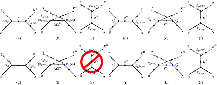
Figure 1: Feynman diagrams for the $\gamma p\to K^{+}\Lambda$ [(a)$-$(f)] and the $\gamma n\to K^{0}\Lambda$ [(g)$-$(l)] photoproductions. For the sake of brevity the contact diagrams for preserving the gauge invariance in the pseudovector theory, or in the pseudoscalar theory after including the hadronic form factors, are not displayed in this figure.

The reaction kinematics is defined through the general $K\Lambda$ photoproduction process,

$$\gamma(k)+N(p_{N})\to K(q)+\Lambda(p_{\Lambda})~{}.$$ (1)

The relevant Feynman diagrams for the two processes considered in this work are depicted in Fig. 1. The basic effective Lagrangian for the kaon-hyperon-nucleon interaction can be written as

$${\cal L}_{K\Lambda N}=g_{K\Lambda N}\,{\bar{\psi}}_{N}\gamma_{5}\,\psi_{\Lambda}\,\Phi_{K},$$ (2)

and

$${\cal L}_{K\Sigma^{0}N}=g_{K\Sigma^{0}N}\,{\bar{\psi}}_{N}\gamma_{5}\,\psi_{\Sigma^{0}}\,\Phi_{K},$$ (3)

where $\psi_{N}$ and $\psi_{\Lambda}$ ($\psi_{\Sigma^{0}}$) are the spinor fields of nucleon and $\Lambda$ ($\Sigma^{0}$), respectively, and $\Phi_{K}$ is the pseudoscalar field of the kaon.

The electromagnetic interactions for the nucleon ($N$), hyperon ($\Lambda$ and $\Sigma^{0}$), and kaon read

$${\cal L}_{\gamma NN} = e{\bar{\psi}}_{N}\left(-Q_{N}\gamma_{\mu}A^{\mu}+\frac{\kappa_{N}}{4m_{N}}\sigma_{\mu\nu}\,F^{\mu\nu}\right)\psi_{N},~{}~{}$$ (4)

$${\cal L}_{\gamma\Lambda\Lambda} = \frac{e\kappa_{\Lambda}}{4m_{\Lambda}}{\bar{\psi}}_{\Lambda}\sigma_{\mu\nu}\,F^{\mu\nu}\psi_{\Lambda},$$ (5)

$${\cal L}_{\gamma\Sigma^{0}\Lambda} = \frac{e\kappa_{\rm T}}{2(m_{\Lambda}+m_{\Sigma^{0}})}{\bar{\psi}}_{\Lambda}\sigma_{\mu\nu}\,F^{\mu\nu}\psi_{\Sigma^{0}}~{},$$ (6)

$${\cal L}_{\gamma KK} = g_{\gamma KK}Q_{K}\left\{{\bar{\Phi}}_{K}(\partial_{\mu}\Phi_{K})-(\partial_{\mu}{\bar{\Phi}_{K}})\Phi_{K}\right\}A^{\mu},~{}~{}$$ (7)

where $Q_{N}$ ($Q_{K}$) is the charge of the nucleon (kaon) in the unit of positron charge, $F^{\mu\nu}=\partial^{\mu}A^{\nu}-\partial^{\nu}A^{\mu}$, while other terms are self-explanatory.

For the interactions of excited kaons the Lagrangians read Kim:2018qfu

$${\cal L}_{K^{*}\Lambda N} = {\bar{\psi}}_{N}\left\{-ig^{V}_{K^{*}\Lambda N}\gamma^{\mu}\psi_{\Lambda}\right.$$ (8)

$$\left.+\frac{g^{T}_{K^{*}\Lambda N}}{m_{N}+m_{\Lambda}}\sigma_{\mu\nu}\,\psi_{\Lambda}\partial^{\nu}\right\}\Phi_{\mu}^{K^{*}}+{\rm H.c.},$$

and

$${\cal L}_{\gamma KK^{*}} = g_{\gamma KK^{*}}\epsilon_{\mu\nu\rho\sigma}\,\partial^{\mu}A^{\nu}$$ (9)

$$\times\left\{(\partial^{\rho}{\bar{\Phi}}^{\sigma}_{K^{*}})\Phi_{K}+{\bar{\Phi}}_{K}(\partial^{\rho}\Phi^{\sigma}_{K^{*}})\right\},~{}$$

where $\epsilon_{\mu\nu\rho\sigma}$ is the four-dimensional Levi-Civita tensor with $\epsilon_{0123}=+1$.

In the case of spin-1/2 nucleon resonances we also use the standard interaction Lagrangian, i.e., Mart:2013ida

$${\cal L}_{K\Lambda N^{*}}=g_{K\Lambda N^{*}}{\bar{\psi}}_{\Lambda}\gamma_{5}\,\psi_{N^{*}}\Phi_{K}+{\rm H.c.},$$ (10)

for the hadronic transition. For the magnetic transition the Lagrangian reads Mart:2013ida

$${\cal L}_{\gamma NN^{*}}=\frac{eg_{\gamma NN^{*}}}{2(m_{N}+m_{N^{*}})}{\bar{\psi}}_{N^{*}}\sigma_{\mu\nu}\,F^{\mu\nu}\,\psi_{N}+{\rm H.c.},$$ (11)

where $g_{\gamma NN^{*}}$ is the transition magnetic moment of the resonance. In our standard notation, the propagator of spin-1/2 nucleon resonance reads $(\not{p}_{N^{*}}+m_{N^{*}})/(s-m_{N^{*}}^{2}+im_{N^{*}}\Gamma_{N^{*}})$, where $s$ is the Mandelstam variable and $\Gamma_{N^{*}}$ is the resonance width. Note that according to Eq. (1) we have

$$s = p_{N^{*}}^{2}~{}=~{}(k+p_{N})^{2}~{}=~{}W^{2}~{},$$ (12)

$$t = (k-q)^{2}~{},$$ (13)

$$u = (k-p_{\Lambda})^{2}~{}.$$ (14)

For the nucleon resonances with spins 3/2 and higher we use the consistent interaction Lagrangian described in Ref. Clymton:2017nvp . In this case the hadronic interaction Lagrangian of the spin-($n+1/2$) nucleon resonance can be written as

$$\mathcal{L}_{K\Lambda N^{*}} = \frac{g_{K\Lambda N^{*}}}{m_{N^{*}}^{2n+1}}\,\epsilon^{\mu\nu_{n}\alpha\beta}\,\partial^{\nu_{1}}\cdots\partial^{\nu_{n-1}}\bar{\psi}_{\Lambda}\,\partial_{\beta}\Phi^{*}_{K}\,\gamma_{5}\,\gamma_{\alpha}\,$$ (15)

$$\times\partial_{\mu}\,\Psi_{\nu_{1}\cdots\nu_{n}}\,+\mathrm{H.c.}~{},$$

while the corresponding magnetic transition Lagrangian reads

$$\mathcal{L}_{\gamma NN^{*}} = \frac{e}{m_{N^{*}}^{2n+1}}\bar{\Psi}^{\beta_{1}\cdots\beta_{n}}\bigl{\{}g_{\gamma NN^{*}}^{(1)}\,\epsilon_{\mu\nu\alpha\beta_{n}}\partial^{\alpha}\psi_{N}$$ (16)

$$+g_{\gamma NN^{*}}^{(2)}\,\gamma_{5}\,g_{\beta_{n}\nu}\partial_{\mu}\psi_{N}$$

$$+g_{\gamma NN^{*}}^{(3)}\,\gamma_{\mu}\,\gamma^{\rho}\,\epsilon_{\rho\nu\alpha\beta_{n}}\partial^{\alpha}\psi_{N}$$

$$+g_{\gamma NN^{*}}^{(4)}\,\gamma_{5}\,\gamma_{\mu}\,\gamma^{\rho}\,(\partial_{\rho}g_{\nu\beta_{n}}-\partial_{\nu}g_{\rho\beta_{n}})\psi_{N}\bigr{\}}$$

$$\times\partial_{\beta_{1}}\cdots\partial_{\beta_{n-1}}F^{\mu\nu}+\mathrm{H.c.}$$

Note that in Eqs. (15) and (16) we have introduced $\Psi_{\mu_{1}\cdots\mu_{n}}$ to denote the massive Rarita-Schwinger field of $N^{*}$. Furthermore, Eq. (16) also indicates that, in general, we have four transition moments for the magnetic excitations of nucleon resonances with spins 3/2 or higher, which are indicated by $g_{\gamma NN^{*}}^{(1)},\cdots,g_{\gamma NN^{*}}^{(4)}$. Due to the lack of information on these transition moments, for all nucleon resonances we can only extract the product of this moment and the hadronic coupling constant, i.e.,

$$G_{N^{*}}^{(i)} \equiv G_{K\Lambda N^{*}}^{(i)}=g_{\gamma NN^{*}}^{(i)}\,g_{K\Lambda N^{*}}~{},$$ (17)

from fitting to experimental data. Note that Eq. (17), but without index $i$, is also used for the spin-1/2 nucleon resonance described by Eqs. (10) and (11).

II.2 Propagators

The propagators for spin-$(n+1/2)$ nucleon resonances can be obtained from Ref. Vrancx:2011qv , i.e.,

$$P^{\mu_{1}\cdots\mu_{n},\nu_{1}\cdots\nu_{n}}_{(n+1/2)}(p_{N^{*}})$$

$$=\,\frac{\not{p}_{N^{*}}+m_{N^{*}}}{p_{N^{*}}^{2}-m_{N^{*}}^{2}+im_{N^{*}}\Gamma_{N^{*}}}\,\widetilde{\mathcal{P}}^{\mu_{1}\cdots\mu_{n},\nu_{1}\cdots\nu_{n}}_{(n+1/2)}(p_{N^{*}}),~{}~{}~{}$$ (18)

where $\widetilde{\mathcal{P}}^{\mu_{1}\cdots\mu_{n},\nu_{1}\cdots\nu_{n}}_{(n+1/2)}(p_{N^{*}})$ denotes the on-shell projection operator that is obtained from the off-shell projection operator ${\mathcal{P}}^{\mu_{1}\cdots\mu_{n},\nu_{1}\cdots\nu_{n}}_{(n+1/2)}(p_{N^{*}})$ with the replacements $\not{p}_{N^{*}}\to m_{N^{*}}$ and ${p}_{N^{*}}^{2}\to m_{N^{*}}^{2}$. For example, the propagator for spin-7/2 nucleon resonance reads Clymton:2017nvp

$$\mathop{P^{7/2}_{\mu\mu_{1}\mu_{2}}}_{\;\;\nu\nu_{1}\nu_{2}}=\frac{s^{3}}{m_{N^{*}}^{6}}\frac{(\not{p}_{N^{*}}+m_{N^{*}})}{(s-m_{N^{*}}^{2}+im_{N^{*}}\Gamma_{N^{*}})}\mathop{\mathcal{P}^{7/2}_{\mu\mu_{1}\mu_{2}}}_{\;\;\nu\nu_{1}\nu_{2}}~{},$$ (19)

where the spin-7/2 projection operator is given by Clymton:2017nvp

$$\mathop{\mathcal{P}^{7/2}_{\mu_{1}\mu_{2}\mu_{3}}}_{\;\;\nu_{1}\nu_{2}\nu_{3}} = \frac{1}{36}\sum_{\mathrm{P}(\mu),\mathrm{P}(\nu)}\Bigl{\{}P_{\mu_{1}\nu_{1}}P_{\mu_{2}\nu_{2}}P_{\mu_{3}\nu_{3}}$$ (20)

$$-\textstyle{\frac{3}{7}}P_{\mu_{1}\mu_{2}}P_{\nu_{1}\nu_{2}}P_{\mu_{3}\nu_{3}}$$

$$+\textstyle{\frac{3}{7}}\gamma^{\,\rho}\gamma^{\sigma}P_{\mu_{1}\rho}P_{\nu_{1}\sigma}P_{\mu_{2}\nu_{2}}P_{\mu_{3}\nu_{3}}$$

$$-\textstyle{\frac{3}{35}}\gamma^{\,\rho}\gamma^{\sigma}P_{\mu_{1}\rho}P_{\nu_{1}\sigma}P_{\mu_{2}\mu_{3}}P_{\nu_{2}\nu_{3}}\Bigr{\}}~{},$$

where $\mathrm{P}(\mu)$ and $\mathrm{P}(\nu)$ indicate the permutations of all possible $\mu$ and $\nu$ indices, respectively, while $P_{\mu\nu}=-g_{\mu\nu}+p_{N^{*}\mu}p_{N^{*}\nu}/s$.

The interaction Lagrangians described above are designed for positive parity intermediate states. For the negative parity states we have to modify these Lagrangians as explained in Ref. Clymton:2017nvp .

II.3 Differences between $K^{+}\Lambda$ and $K^{0}\Lambda$ photoproductions

The appropriate Feynman diagrams for both $K^{+}\Lambda$ and $K^{0}\Lambda$ channels are depicted in Fig. 1, where the corresponding Born terms are displayed by the diagrams (a)$-$(c) and (g) and (h) of Fig. 1, respectively. From Fig. 1 it is clear that the difference between the two processes originates from the charge of participating nucleon and kaon. Therefore, the hadronic coupling constants in both reactions can be related by using isospin symmetry. Since the $\Lambda$ hyperon is an SU(3) isosinglet, the symmetry prescribes that the corresponding $N\to K\Lambda$ hadronic couplings in both channels are equal, i.e.,

$$g_{K^{+}\Lambda p}=g_{K^{0}\Lambda n}~{}.$$ (21)

As shown by the diagrams (b) and (h) in Fig. 1, the $\Sigma^{0}$ exchange is also allowed in the $u$-channel. However, different from $\Lambda$ hyperon, $\Sigma$ is an SU(3) isotriplet and as a consequence we obtain Mart:1995wu

$$g_{K^{+}\Sigma^{0}p}=-g_{K^{0}\Sigma^{0}n}.~{}$$ (22)

In the $N\to K^{*}\Lambda$ vertex the isospin symmetry also leads to a similar relation to that of Eq. (21), i.e.,

$$g^{V,T}_{K^{*+}\Lambda p}=g^{V,T}_{K^{*0}\Lambda n}.$$ (23)

Equation (23) is also valid for the vector meson $K_{1}(1270)$.

Similar to Eqs. (21) and (22) the application of isospin symmetry in the $N^{*}\to K\Lambda$ and $N\to KY^{*}$ vertices results in [diagrams (d) and (j)]

$$g_{K^{+}\Lambda N^{*}}=g_{K^{0}\Lambda N^{*}}~{},$$ (24)

and with $Y^{*}=\Lambda^{*},\Sigma^{0*}$ [diagrams (e) and (k)]

$$g_{K^{+}\Lambda^{*}p}=g_{K^{0}\Lambda^{*}n}~{}~{}~{},~{}~{}~{}g_{K^{+}\Sigma^{0*}p}=-g_{K^{0}\Sigma^{0*}n}~{}.$$ (25)

The electromagnetic vertices for the proton, neutron, $\Lambda$, and $\Sigma^{0}$ exchanges shown by the diagrams (a) and (b) in Fig. 1 are elementary and do not need explanation. The $K^{+}$ and $K^{0}$ intermediate states as given by the diagrams (c) and (i) are also the same. Since the real photon cannot interact with a neutral kaon, the $K^{0}$ intermediate state is not allowed in the amplitude of the $K^{0}\Lambda$ photoproduction, in contrast to the case of $K^{+}\Lambda$ photoproduction.

In the case of spin-1/2 nucleon resonances the transition moments in the two channels [diagrams (d) and (j)] can be related to the corresponding resonance helicity amplitudes $A_{1/2}$, i.e., Mart:1995wu

$$r_{N^{*}}\equiv\frac{g_{\gamma nN^{*}}}{g_{\gamma pN^{*}}}=\frac{A_{1/2}^{n}}{A_{1/2}^{p}}~{}.$$ (26)

For the nucleon resonances with spins 3/2 and higher the corresponding relations are more complicated Clymton:2017nvp . Furthermore, the corresponding values of neutron helicity amplitudes $A_{1/2}^{n}$ and $A_{3/2}^{n}$ are mostly unknown. Therefore, in this work these values are considered as free parameters during the fitting process and for this purpose we define the ratio [see Eq. (16)]

$$r_{N^{*}}^{(i)}\equiv\frac{g_{\gamma nN^{*}}^{(i)}}{g_{\gamma pN^{*}}^{(i)}}~{}.$$ (27)

For hyperon resonances fortunately the transition moments in the two channels are identical, as shown by the diagrams (e) and (k) in Fig. 1.

Finally, the kaon resonance transition moments shown by the diagrams (f) and (l) in Fig. 1 can be related to its decay width. The result for $K^{*}(892)$ is Mart:1995wu

$$r_{K^{0}}\equiv g_{K^{*0}K^{0}\gamma}/g_{K^{*+}K^{+}\gamma}=-1.53\pm 0.20\,.$$ (28)

For the vector meson $K_{1}(1270)$ the corresponding value is not available and, therefore, we consider it also as a fitting parameter, i.e.,

$$r_{K_{1}}\equiv g_{K^{0}_{1}K^{0}\gamma}/g_{K^{+}_{1}K^{+}\gamma}\,.$$ (29)

II.4 Nucleon and hyperon resonances used in the present analysis

The number of nucleon resonances used in our analysis is limited by the energy range of experimental data in our database. As in the previous work Clymton:2017nvp we further constrain the number by excluding the resonances with one-star rating in the overall status given by PDG. The result is listed in Table 1 along with their properties obtained from the PDG estimates pdg . There are 18 nucleon resonances involved in this analysis with spins up to 9/2. Since the estimated mass and width of each resonance have error bars, during the fitting process we vary their values within these error bars. Note that, in contrast to the pion and $K\Sigma$ photoproductions, delta resonances are not allowed in the $K^{+}\Lambda$ photoproduction due to the isospin conservation.

Table 1: Properties of the nucleon resonances used in the present analysis. Data are taken from the Review of Particle Properties of the PDG pdg .

Resonance	$J^{P}$	$M$ (MeV)	$\Gamma$ (MeV)	Status
$N(1440)P_{11}$	$1/2^{+}$	1410 to 1470	250 to 450	****
$N(1520)D_{13}$	$3/2^{-}$	1510 to 1520	100 to 120	****
$N(1535)S_{11}$	$1/2^{-}$	1515 to 1545	125 to 175	****
$N(1650)S_{11}$	$1/2^{-}$	1645 to 1670	$104\pm 10$	****
$N(1675)D_{15}$	$5/2^{-}$	1670 to 1680	$120\pm 15$	****
$N(1680)F_{15}$	$5/2^{+}$	1680 to 1690	$118\pm 6$	***
$N(1700)D_{13}$	$3/2^{-}$	1650 to 1750	100 to 250	***
$N(1710)P_{11}$	$1/2^{+}$	1680 to 1740	80 to 200	****
$N(1720)P_{13}$	$3/2^{+}$	1680 to 1750	150 to 400	****
$N(1860)F_{15}$	$5/2^{+}$	$1860^{+100}_{-40}$	$270^{+140}_{-50}$	**
$N(1875)D_{13}$	$3/2^{-}$	1850 to 1920	120 to 250	***
$N(1880)P_{11}$	$1/2^{+}$	1830 to 1930	200 to 400	***
$N(1895)S_{11}$	$1/2^{-}$	1870 to 1920	80 to 200	****
$N(1900)P_{13}$	$3/2^{+}$	1890 to 1950	100 to 320	****
$N(1990)F_{17}$	$7/2^{+}$	1950 to 2100	200 to 400	**
$N(2000)F_{15}$	$5/2^{+}$	$2060\pm 30$	$390\pm 55$	**
$N(2060)D_{15}$	$5/2^{-}$	2030 to 2200	300 to 450	***
$N(2120)D_{13}$	$3/2^{-}$	2060 to 2160	260 to 360	***
$N(2190)G_{17}$	$7/2^{-}$	2140 to 2220	300 to 500	****
$N(2220)H_{19}$	$9/2^{+}$	2200 to 2300	350 to 500	****
$N(2250)G_{19}$	$9/2^{-}$	2250 to 2320	300 to 600	****

Table 2: Properties of the hyperon resonances used in the present analysis. Data are taken from the Review of Particle Properties of the PDG pdg .

Resonance	$J^{P}$	$M$ (MeV)	$\Gamma$ (MeV)	Status
$\Lambda(1405)S_{01}$	$1/2^{-}$	$1405.1^{+1.3}_{-1.0}$	$50.5\pm 2.0$	****
$\Lambda(1520)D_{03}$	$3/2^{-}$	$1517^{+4}_{-4}$	$15^{+10}_{-8}$	****
$\Lambda(1600)P_{01}$	$1/2^{+}$	$1544^{+3}_{-3}$	$112^{+12}_{-2}$	***
$\Lambda(1670)S_{01}$	$1/2^{-}$	$1669^{+3}_{-8}$	$19^{+18}_{-2}$	****
$\Lambda(1690)D_{03}$	$3/2^{-}$	$1697^{+6}_{-6}$	$65\pm 14$	****
$\Lambda(1800)S_{01}$	$1/2^{-}$	1720 to 1850	200 to 400	***
$\Lambda(1810)P_{01}$	$1/2^{+}$	1750 to 1850	50 to 250	***
$\Lambda(1890)P_{03}$	$3/2^{+}$	1850 to 1910	60 to 200	****
$\Sigma(1385)P_{13}$	$3/2^{+}$	$1382.80\pm 0.35$	$36.0\pm 0.7$	****
$\Sigma(1660)P_{11}$	$1/2^{+}$	1630 to 1690	40 to 200	***
$\Sigma(1670)D_{13}$	$3/2^{-}$	1665 to 1685	40 to 80	****
$\Sigma(1750)S_{11}$	$1/2^{-}$	1730 to 1800	60 to 160	***
$\Sigma(1880)P_{11}$	$1/2^{+}$	1880	$300\pm 59$	**
$\Sigma(1940)D_{13}$	$3/2^{-}$	$1941\pm 18$	$400\pm 49$	*
$\Sigma(2080)P_{13}$	$3/2^{+}$	2080	$186\pm 48$	**

For the hyperon resonances we limit the number of the used resonances by excluding those with spins higher than 3/2. They are listed in Table 2. Note that in the literatures these resonances are considered as a part of the background, since their squared momentum is $u$, instead of $s$.

II.5 Experimental data and fitted observables

Table 3: Observables and experimental data used in the previous and present studies. Channels 1 and 2 refer to the $\gamma p\to K^{+}\Lambda$ and $\gamma n\to K^{0}\Lambda$ channels, respectively. Columns M1, M2, and M3 indicate the data set used in the models M1, M2, and M3, respectively. The data set used in the previous model Clymton:2017nvp and updated to include the CLAS 2016 double polarization data paterson is indicated by M0 samson_thesis . Note that, except for channel 2, all data sets listed in this table have been given in our previous work Mart:2017mwj .

Collaboration	Observable	Symbol	$N$	Channel	M0	M1	M2	M3	Reference
CLAS 2006	Differential cross section	$d\sigma/d\Omega$	1377	1	✓	✓	✓	✓	Bradford:2005pt
	Recoil polarization	$P$	233	1	✓	✓	✓	✓	Bradford:2005pt
LEPS 2006	Differential cross section	$d\sigma/d\Omega$	$54$	1	✓	✓	✓	✓	Sumihama06
	Photon asymmetry	$\Sigma$	$30$	1	✓	✓	✓	✓	Sumihama06
GRAAL 2007	Recoil polarization	$P$	$66$	1	✓	✓	✓	✓	lleres:2007
	Photon asymmetry	$\Sigma$	$66$	1	✓	✓	✓	✓	lleres:2007
LEPS 2007	Differential cross section	$d\sigma/d\Omega$	$12$	1	✓	✓	✓	✓	Hicks_2007
CLAS 2007	Beam-Recoil polarization	$C_{x}$	$159$	1	✓	✓	✓	✓	Bradford:2006ba
	Beam-Recoil polarization	$C_{z}$	160	1	✓	✓	✓	✓	Bradford:2006ba
GRAAL 2009	Target asymmetry	$\Sigma$	$66$	1	✓	✓	✓	✓	lleres:2009
	Beam-Recoil polarization	$O_{x^{\prime}}$	$66$	1	✓	✓	✓	✓	lleres:2009
	Beam-Recoil polarization	$O_{z^{\prime}}$	$66$	1	✓	✓	✓	✓	lleres:2009
CLAS 2010	Differential cross section	$d\sigma/d\Omega$	2066	1	✓	✓	✓	✓	mcCracken
	Recoil polarization	$P$	1707	1	✓	✓	✓	✓	mcCracken
Crystal Ball 2014	Differential cross section	$d\sigma/d\Omega$	1301	1	✓	✓	✓	✓	Jude:2013jzs
CLAS 2016	Recoil polarization	$P$	$314$	1	✓	✓	✓	✓	paterson
	Photon asymmetry	$\Sigma$	$314$	1	✓	✓	✓	✓	paterson
	Target asymmetry	$T$	$314$	1	✓	✓	✓	✓	paterson
	Beam-Recoil polarization	$O_{x}$	$314$	1	✓	✓	✓	✓	paterson
	Beam-Recoil polarization	$O_{z}$	$314$	1	✓	✓	✓	✓	paterson
CLAS 2017	Differential cross section	$d\sigma/d\Omega$	$361$	2	$\cdots$	✓	$\cdots$	✓	Compton:2017xkt
MAMI 2018	Differential cross section	$d\sigma/d\Omega$	$60$	2	$\cdots$	$\cdots$	✓	✓	Akondi:2018shh
Total number of data			9424		$9003$	$9364$	$9063$	$9424$

As explained in the introduction the present model is based on our previous covariant isobar one Clymton:2017nvp that fits nearly 7400 experimental data points of the $\gamma p\to K^{+}\Lambda$ channel. However, we notice that additional experimental data for double polarization observables paterson consisting of 1574 data points appeared almost at the same time of the publication of Ref. Clymton:2017nvp . Thus, in total the number of $\gamma p\to K^{+}\Lambda$ data points is 9003. At this stage it is important to mention that a new determination of $\Lambda$ decay parameter $\alpha_{-}$ has been reported in Ref. Ireland:2019uja . The new value is significantly larger than the standard one tabulated in the Review of Particle Properties of PDG pdg and may affect the obtained experimental data for the recoil polarization. Note that, different from our previous covariant isobar model, our recent multipole analysis Mart:2017mwj has used 9003 data points. As a consequence, we have to refit our previous covariant model by including these double polarization data in the fitting database. The result is denoted by M0 and is discussed in Sec. III. The detailed data sets used in this model are listed in Table 3.

As shown in Table 3 the new $\gamma n\to K^{0}\Lambda$ data consist of 401 data points obtained from the CLAS 2017 Compton:2017xkt and MAMI 2018 Akondi:2018shh collaborations. Our recent analysis on this isospin channel indicates that the two data sets show a sizable discrepancy Mart:ptep2019 . To investigate the effect of these two data sets on our model we propose three different models that fit all $\gamma p\to K^{+}\Lambda$ data along with the $\gamma n\to K^{0}\Lambda$ data obtained from the CLAS 2017, MAMI 2018, and both CLAS 2017 and MAMI 2018 collaborations. In Table 3 the three different models are denoted by M1, M2, and M3, respectively.

II.6 Calculation of observables

For the convenience of the reader we briefly summarize the formulas used for calculating the observables. Since we are working with photoproduction the formalism is further simplified by the fact that $k^{2}=k\cdot\epsilon=0$. The transition amplitude ${\cal M}$ obtained from the Feynman diagrams given in Fig. 1 can be decomposed into the gauge and Lorentz invariant matrices $M_{i}$ Clymton:2017nvp ,

$${\cal M} = {\bar{u}}_{\Lambda}\sum_{i=1}^{4}A_{i}(s,t,u)\,M_{i}\,u_{N}~{},$$ (30)

where $s$, $t$, and $u$ are the Mandelstam variables given in Eqs. (12)$-$(14) and the four gauge and Lorentz invariant matrices $M_{i}$ are given by

$$M_{1} = \gamma_{5}\,\epsilon\!\!/k\!\!\!/~{},$$ (31)

$$M_{2} = 2\gamma_{5}\left(q\cdot\epsilon P\cdot k-q\cdot kP\cdot\epsilon\right)~{},$$ (32)

$$M_{3} = \gamma_{5}\left(q\cdot k\epsilon\!\!/-q\cdot\epsilon k\!\!\!/\right)~{},$$ (33)

$$M_{4} = i\epsilon_{\mu\nu\rho\sigma}\gamma^{\mu}q^{\nu}\epsilon^{\rho}k^{\sigma}~{},$$ (34)

with $P=\frac{1}{2}(p_{N}+p_{\Lambda})$ and $\epsilon$ being the photon polarization. All observables required in the present analysis can be calculated from $A_{i}$ extracted from Eq. (30). The relations between these observables and $A_{i}$ can be found, e.g., in Ref. Knochlein:1995qz .

In the hadronic vertices of background and resonance terms we insert hadronic form factors in the form of Haberzettl:1998eq

$$F(\Lambda,x) = \frac{\Lambda^{4}}{\Lambda^{4}+(x-m_{x}^{2})^{2}}~{},$$ (35)

where $x$, $\Lambda$, and $m_{x}$ are the corresponding Mandelstam variables ($s$, $t$, or $u$), the form factor cutoff, and the mass of intermediate state, respectively. Note that in the background terms the inclusion of hadronic form factors destroys the gauge invariance of the amplitude. To restore the gauge invariance we utilize the Haberzettl method Haberzettl:1998eq with the cost of adding two extra parameters originating from the freedom of choosing the form factor for the electric amplitude $A_{2}$ in Eq. (30). As in the previous study we use Haberzettl:1998eq

$${\tilde{F}}(\Lambda,s,t,u) = F(\Lambda,s)\sin^{2}\theta_{\rm had}\cos^{2}\phi_{\rm had}$$ (36)

$$+F(\Lambda,u)\sin^{2}\theta_{\rm had}\sin^{2}\phi_{\rm had}$$

$$+F(\Lambda,t)\cos^{2}\theta_{\rm had}~{},$$

where the combination of the form factors in Eq. (36) ensures the correct normalization, i.e., ${\tilde{F}}(\Lambda,m_{s}^{2},m_{t}^{2},m_{u}^{2})=1$. In the present work we extract both $\theta_{\rm had}$ and $\phi_{\rm had}$ from the fitting process. Our previous investigations indicate that the background and resonance amplitudes require different suppressions from the form factors. Therefore, in the present work we separate these form factors by defining different cutoffs for these amplitudes, i.e., $\Lambda_{\rm B}$ and $\Lambda_{\rm R}$, respectively.

III RESULTS AND DISCUSSION

III.1 Results from previous works

The results from our previous analyses are shown in Fig. 2. For the $\gamma p\to K^{+}\Lambda$ channel, except in the case of Kaon-Maid, it is clear that our previous calculations can nicely reproduce the experimental data. As shown in the top panel of Fig. 2 Kaon-Maid cannot reproduce the data because it was fitted to the SAPHIR data Tran:1998 ; Glander:2003jw which are smaller than the CLAS data for $W\geq 1.7$ GeV. This problem has been thoroughly discussed in Ref. Mart:2006dk . For $W\geq 2.3$ GeV both multipole and isobar models seem to underpredict the CLAS total cross section data. However, this problem does not appear in most of the differential cross section data used in the fitting database because they are in fact smaller than the CLAS 2006 ones (see Fig. 3 and the corresponding discussion below). Thus, we believe that the smaller calculated total cross section shown in this kinematics is natural

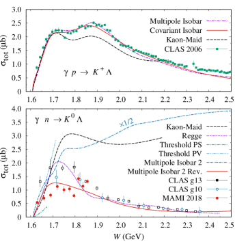
Figure 2: (Top panel) The $K^{+}\Lambda$ photoproduction total cross section as a function of the total c.m. energy $W$. Experimental data are taken from the CLAS 2006 collaboration Bradford:2005pt . The dot-dashed curve shows the result of the recent multipole analysis of the $\gamma p\to K^{+}\Lambda$ photoproduction data Mart:2017mwj , and the dashed curve is taken from the Kaon-Maid model kaon-maid , whereas the solid curve is obtained from the previous effective Lagrangian model with nucleon spins up to 9/2 Clymton:2017nvp . (Bottom panel) As in the top panel but for the $\gamma n\to K^{0}\Lambda$ photoproduction. Experimental data are taken from the CLAS g10 and g13 experiments Compton:2017xkt , as well as from the MAMI 2018 collaboration Akondi:2018shh . The dashed and dotted curves show the result of Kaon-Maid kaon-maid and recent effective-Lagrangian-Regge Kim:2018qfu models, respectively. The dot-dashed and dot-dot-dashed curves are obtained from the photoproduction analysis at threshold by using PS and PV couplings mart_thr , respectively, whereas the the dot-dash-dashed and solid curves exhibit the prediction of the recent multipole model Mart:2017xtf and the corresponding revised version Mart:ptep2019 . Note that the dot-dash-dashed curve has been rescaled by a factor of 1/2 to fit in the same plot. All data shown in this figure were not used in the fitting process; they are shown here only for comparison.

In contrast to the $\gamma p\to K^{+}\Lambda$ channel, as shown in the bottom panel of Fig. 2 the predicted and calculated $\gamma n\to K^{0}\Lambda$ total cross sections vary significantly. This is understandable because without fitting to the experimental data the isospin symmetry relations given by Eqs. (21)-(29) could lead to a large transition amplitude that eventually yields a huge cross section. We note that this situation happens in the Kaon-Maid and our previous Mart:2017xtf models. However, in the latter it has been shown that the model can be significantly improved by including the $\gamma n\to K^{0}\Lambda$ differential cross section data in the fitting database Mart:ptep2019 , although as shown by the solid line in the bottom panel of Fig. 2 this model exhibits a compromise result since it was fitted to both CLAS and MAMI data.

In spite of the wild variation of the models shown in the bottom panel of Fig. 2, within the experimental error bars all models are still in agreement with the trend of experimental data in the low energy region, i.e., from threshold up to $W\approx 1.66$ GeV. Especially interesting is the result of our previous investigation that explores the difference between the use of PS and PV couplings in the threshold region mart_k0lambda . Although it was believed that the PS model works better than the PV one, comparison between the two models given in the bottom panel of Fig. 2 indicates that PV coupling yields a better agreement with the data in the low energy region. The PS coupling yields a much smaller total cross section; still smaller than the data given by the MAMI 2018 collaboration. Nevertheless, a firm conclusion to this end cannot be easily drawn before we can solve the problem of discrepancy between the CLAS and MAMI data. We discuss this problem in the following subsection.

III.2 Results from the present analysis

Table 4: Coupling constants and some parameters of the background terms. See Ref. Mart:2015jof for the notation of the parameters.

Parameter	M0	M1	M2	M3
$g_{K\Lambda N}/\sqrt{4\pi}$	$-3.43$	$-3.00$	$-3.96$	$-3.40$
$g_{K\Sigma N}/\sqrt{4\pi}$	$1.30$	$1.30$	$1.30$	$1.30$
$G^{V}_{K^{*}}/4\pi$	$0.22$	$0.13$	$0.22$	$0.18$
$G^{T}_{K^{*}}/4\pi$	$0.37$	$0.17$	$0.36$	$0.18$
$G^{V}_{K_{1}}/4\pi$	$-0.07$	$0.13$	$-0.25$	$-0.17$
$G^{T}_{K_{1}}/4\pi$	$4.40$	$3.89$	$4.54$	$4.48$
$r_{K_{1}K\gamma}$	$0.00$	$0.65$	$-0.52$	$0.69$
$\theta_{\rm had}$ (deg.)	$90.0$	$90.0$	$90.0$	$90.0$
$\phi_{\rm had}$ (deg)	$144.6$	$0.0$	$60.6$	$8.0$
$\Lambda_{\rm B}$ (GeV)	$0.70$	$0.70$	$0.70$	$0.70$
$\Lambda_{\rm R}$ (GeV)	$1.07$	$1.10$	$1.07$	$1.09$
$\chi^{2}$	13433	13867	13473	14068
$N_{\rm data}$	9003	9364	9063	9424
$N_{\rm par.}$	184	247	247	247
$\chi^{2}/N_{\rm dof}$	1.52	1.52	1.53	1.53

Table 5: Properties of the nucleon resonances extracted from different models. Note that $G^{(i)}_{N^{*}}$ and $r^{(i)}_{N^{*}}$, with $i=1,\cdots,4$, are defined in Eqs. (17) and (27), respectively.

Resonance	Model	$m_{N^{*}}$	$\Gamma_{N^{*}}$	$G^{(1)}_{N^{*}}$	$G^{(2)}_{N^{*}}$	$G^{(3)}_{N^{*}}$	$G^{(4)}_{N^{*}}$	$r^{(1)}_{N^{*}}$	$r^{(2)}_{N^{*}}$	$r^{(3)}_{N^{*}}$	$r^{(4)}_{N^{*}}$
		(MeV)	(MeV)
$N(1440)P_{11}$	M0	$1410$	$450$	$0.77$	$\cdots$	$\cdots$	$\cdots$	$\cdots$	$\cdots$	$\cdots$	$\cdots$
	M1	$1410$	$450$	$0.64$	$\cdots$	$\cdots$	$\cdots$	$\cdots$	$\cdots$	$\cdots$	$\cdots$
	M2	$1410$	$450$	$0.67$	$\cdots$	$\cdots$	$\cdots$	$\cdots$	$\cdots$	$\cdots$	$\cdots$
	M3	$1410$	$450$	$0.80$	$\cdots$	$\cdots$	$\cdots$	$\cdots$	$\cdots$	$\cdots$	$\cdots$
$N(1520)D_{13}$	M0	$1520$	$125$	$0.12$	$-0.85$	$-0.09$	$0.25$	$0.00$	$0.00$	$0.00$	$0.00$
	M1	$1520$	$100$	$0.18$	$-1.25$	$-0.01$	$0.41$	$-0.04$	$0.98$	$2.00$	$1.10$
	M2	$1520$	$100$	$0.18$	$-1.43$	$-0.07$	$0.52$	$1.46$	$-0.21$	$1.64$	$-0.31$
	M3	$1520$	$100$	$0.19$	$-1.62$	$-0.04$	$0.59$	$0.36$	$1.58$	$-1.04$	$1.64$
$N(1535)S_{11}$	M0	$1525$	$125$	$-0.11$	$\cdots$	$\cdots$	$\cdots$	$\cdots$	$\cdots$	$\cdots$	$\cdots$
	M1	$1525$	$125$	$-0.10$	$\cdots$	$\cdots$	$\cdots$	$\cdots$	$\cdots$	$\cdots$	$\cdots$
	M2	$1545$	$175$	$0.07$	$\cdots$	$\cdots$	$\cdots$	$\cdots$	$\cdots$	$\cdots$	$\cdots$
	M3	$1545$	$175$	$0.05$	$\cdots$	$\cdots$	$\cdots$	$\cdots$	$\cdots$	$\cdots$	$\cdots$
$N(1650)S_{11}$	M0	$1645$	$150$	$0.15$	$\cdots$	$\cdots$	$\cdots$	$\cdots$	$\cdots$	$\cdots$	$\cdots$
	M1	$1645$	$155$	$0.15$	$\cdots$	$\cdots$	$\cdots$	$\cdots$	$\cdots$	$\cdots$	$\cdots$
	M2	$1645$	$170$	$0.09$	$\cdots$	$\cdots$	$\cdots$	$\cdots$	$\cdots$	$\cdots$	$\cdots$
	M3	$1645$	$159$	$0.09$	$\cdots$	$\cdots$	$\cdots$	$\cdots$	$\cdots$	$\cdots$	$\cdots$
$N(1675)D_{15}$	M0	$1680$	$130$	$-2.87$	$-0.20$	$-2.43$	$0.18$	$0.00$	$0.00$	$0.00$	$0.00$
	M1	$1680$	$130$	$-2.62$	$-0.08$	$-2.25$	$0.13$	$0.65$	$-2.00$	$0.76$	$1.63$
	M2	$1680$	$130$	$-2.74$	$-0.35$	$-2.33$	$0.23$	$1.35$	$-2.00$	$1.19$	$2.00$
	M3	$1680$	$130$	$-2.61$	$-0.33$	$-2.23$	$0.24$	$-0.48$	$1.78$	$-0.54$	$1.88$
$N(1680)F_{15}$	M0	$1690$	$120$	$0.93$	$10.00$	$0.50$	$-4.84$	$0.00$	$0.00$	$0.00$	$0.00$
	M1	$1690$	$120$	$1.02$	$10.00$	$0.70$	$-4.77$	$-1.28$	$1.64$	$-1.42$	$1.41$
	M2	$1690$	$120$	$1.10$	$10.00$	$0.70$	$-4.74$	$2.00$	$-0.59$	$-2.00$	$-0.53$
	M3	$1690$	$120$	$1.01$	$10.00$	$0.62$	$-4.77$	$-1.61$	$0.05$	$-2.00$	$0.04$
$N(1700)D_{13}$	M0	$1732$	$123$	$0.13$	$0.84$	$0.29$	$-0.27$	$0.00$	$0.00$	$0.00$	$0.00$
	M1	$1735$	$130$	$0.15$	$0.77$	$0.29$	$-0.24$	$2.00$	$-0.05$	$0.98$	$0.37$
	M2	$1731$	$113$	$0.09$	$0.72$	$0.24$	$-0.23$	$-1.97$	$-0.74$	$-1.26$	$-1.16$
	M3	$1731$	$102$	$0.06$	$0.62$	$0.19$	$-0.20$	$-2.00$	$-0.05$	$-0.69$	$0.04$
$N(1710)P_{11}$	M0	$1740$	$250$	$0.26$	$\cdots$	$\cdots$	$\cdots$	$\cdots$	$\cdots$	$\cdots$	$\cdots$
	M1	$1740$	$250$	$0.25$	$\cdots$	$\cdots$	$\cdots$	$\cdots$	$\cdots$	$\cdots$	$\cdots$
	M2	$1729$	$250$	$0.30$	$\cdots$	$\cdots$	$\cdots$	$\cdots$	$\cdots$	$\cdots$	$\cdots$
	M3	$1733$	$250$	$0.26$	$\cdots$	$\cdots$	$\cdots$	$\cdots$	$\cdots$	$\cdots$	$\cdots$
$N(1720)P_{13}$	M0	$1700$	$154$	$-0.05$	$0.23$	$-0.02$	$0.00$	$0.00$	$0.00$	$0.00$	$0.00$
	M1	$1700$	$159$	$-0.04$	$0.22$	$-0.01$	$0.01$	$0.12$	$1.34$	$2.00$	$2.00$
	M2	$1700$	$171$	$-0.17$	$0.30$	$-0.11$	$-0.02$	$1.88$	$0.61$	$2.00$	$-0.99$
	M3	$1700$	$189$	$-0.19$	$0.32$	$-0.13$	$-0.02$	$1.70$	$1.36$	$2.00$	$-2.00$
$N(1860)F_{15}$	M0	$1960$	$220$	$-0.99$	$-9.70$	$-0.18$	$4.25$	$0.00$	$0.00$	$0.00$	$0.00$
	M1	$1960$	$220$	$-1.16$	$-8.80$	$-0.35$	$3.84$	$-0.01$	$1.72$	$-0.97$	$1.23$
	M2	$1960$	$220$	$-1.07$	$-9.90$	$-0.32$	$4.24$	$-2.00$	$1.61$	$-2.00$	$0.44$
	M3	$1960$	$220$	$-1.14$	$-9.01$	$-0.30$	$3.90$	$1.26$	$-2.00$	$1.90$	$-1.99$
$N(1875)D_{13}$	M0	$1920$	$320$	$0.06$	$0.40$	$0.09$	$-0.14$	$0.00$	$0.00$	$0.00$	$0.00$
	M1	$1889$	$180$	$0.00$	$0.11$	$0.03$	$-0.03$	$-2.00$	$0.59$	$-2.00$	$-2.00$
	M2	$1873$	$180$	$-0.02$	$0.27$	$0.03$	$-0.10$	$2.00$	$-0.75$	$2.00$	$-1.39$
	M3	$1858$	$180$	$-0.03$	$0.40$	$0.01$	$-0.15$	$-2.00$	$-1.46$	$2.00$	$-2.00$

Table 5: Properties of the nucleon resonances extracted from different models (continued).

Resonance	Model	$m_{N^{*}}$	$\Gamma_{N^{*}}$	$G^{(1)}_{N^{*}}$	$G^{(2)}_{N^{*}}$	$G^{(3)}_{N^{*}}$	$G^{(4)}_{N^{*}}$	$r^{(1)}_{N^{*}}$	$r^{(2)}_{N^{*}}$	$r^{(3)}_{N^{*}}$	$r^{(4)}_{N^{*}}$
		(MeV)	(MeV)
$N(1880)P_{11}$	M0	$1915$	$280$	$0.17$	$\cdots$	$\cdots$	$\cdots$	$0.00$	$\cdots$	$\cdots$	$\cdots$
	M1	$1915$	$280$	$0.19$	$\cdots$	$\cdots$	$\cdots$	$0.96$	$\cdots$	$\cdots$	$\cdots$
	M2	$1915$	$280$	$0.18$	$\cdots$	$\cdots$	$\cdots$	$-0.88$	$\cdots$	$\cdots$	$\cdots$
	M3	$1915$	$280$	$0.18$	$\cdots$	$\cdots$	$\cdots$	$0.16$	$\cdots$	$\cdots$	$\cdots$
$N(1895)S_{11}$	M0	$1893$	$107$	$-0.03$	$\cdots$	$\cdots$	$\cdots$	$0.00$	$\cdots$	$\cdots$	$\cdots$
	M1	$1893$	$106$	$-0.03$	$\cdots$	$\cdots$	$\cdots$	$-0.39$	$\cdots$	$\cdots$	$\cdots$
	M2	$1893$	$110$	$-0.04$	$\cdots$	$\cdots$	$\cdots$	$0.63$	$\cdots$	$\cdots$	$\cdots$
	M3	$1893$	$106$	$-0.03$	$\cdots$	$\cdots$	$\cdots$	$0.14$	$\cdots$	$\cdots$	$\cdots$
$N(1900)P_{13}$	M0	$1930$	$158$	$-0.17$	$0.09$	$-0.13$	$-0.00$	$0.00$	$0.00$	$0.00$	$0.00$
	M1	$1930$	$152$	$-0.16$	$0.08$	$-0.12$	$0.00$	$0.36$	$-0.24$	$0.30$	$2.00$
	M2	$1930$	$161$	$-0.16$	$0.09$	$-0.12$	$-0.00$	$-1.80$	$0.71$	$-1.89$	$2.00$
	M3	$1930$	$151$	$-0.14$	$0.08$	$-0.11$	$-0.00$	$-0.26$	$-0.51$	$-0.28$	$-2.00$
$N(1990)F_{17}$	M0	$1995$	$272$	$-10.00$	$7.15$	$-8.16$	$-1.87$	$0.00$	$0.00$	$0.00$	$0.00$
	M1	$1995$	$314$	$-10.00$	$6.29$	$-7.98$	$-1.54$	$0.38$	$0.76$	$0.43$	$0.14$
	M2	$1995$	$263$	$-10.00$	$6.35$	$-8.09$	$-1.38$	$2.00$	$1.87$	$-0.22$	$-1.95$
	M3	$1995$	$265$	$-10.00$	$5.94$	$-8.03$	$-1.25$	$0.42$	$0.19$	$0.35$	$-1.96$
$N(2000)F_{15}$	M0	$2090$	$335$	$-1.29$	$-10.00$	$-0.66$	$4.44$	$0.00$	$0.00$	$0.00$	$0.00$
	M1	$2090$	$335$	$-1.26$	$-10.00$	$-0.56$	$4.45$	$-0.85$	$0.51$	$-2.00$	$0.78$
	M2	$2090$	$335$	$-1.12$	$-10.00$	$-0.32$	$4.45$	$-2.00$	$-2.00$	$1.93$	$2.00$
	M3	$2090$	$338$	$-1.28$	$-10.00$	$-0.50$	$4.45$	$-0.68$	$1.94$	$0.38$	$1.80$
$N(2060)D_{15}$	M0	$2060$	$450$	$5.05$	$0.42$	$4.16$	$-1.39$	$0.00$	$0.00$	$0.00$	$0.00$
	M1	$2060$	$450$	$5.03$	$0.48$	$4.14$	$-1.33$	$0.27$	$2.00$	$0.40$	$1.23$
	M2	$2060$	$450$	$5.00$	$0.42$	$4.12$	$-1.40$	$-1.94$	$-1.99$	$-1.58$	$-2.00$
	M3	$2060$	$450$	$4.95$	$0.43$	$4.08$	$-1.41$	$-0.93$	$-2.00$	$-0.99$	$0.38$
$N(2120)D_{13}$	M0	$2075$	$375$	$-0.08$	$1.70$	$-0.22$	$-0.67$	$0.00$	$0.00$	$0.00$	$0.00$
	M1	$2075$	$375$	$-0.08$	$1.72$	$-0.22$	$-0.68$	$-0.22$	$0.23$	$0.05$	$0.22$
	M2	$2075$	$375$	$-0.08$	$1.98$	$-0.21$	$-0.79$	$2.00$	$1.88$	$2.00$	$1.77$
	M3	$2075$	$375$	$-0.08$	$1.86$	$-0.23$	$-0.74$	$-2.00$	$0.57$	$-0.20$	$0.59$
$N(2190)G_{17}$	M0	$2175$	$300$	$10.00$	$-10.00$	$3.02$	$6.49$	$0.00$	$0.00$	$0.00$	$0.00$
	M1	$2174$	$300$	$10.00$	$-10.00$	$1.88$	$6.51$	$0.96$	$0.95$	$2.00$	$0.79$
	M2	$2181$	$300$	$10.00$	$-10.00$	$2.54$	$6.45$	$2.00$	$-1.57$	$0.06$	$1.25$
	M3	$2181$	$300$	$10.00$	$-10.00$	$1.78$	$6.34$	$0.58$	$2.00$	$0.87$	$1.55$
$N(2220)H_{19}$	M0	$2200$	$500$	$-10.00$	$-10.00$	$10.00$	$-5.31$	$0.00$	$0.00$	$0.00$	$0.00$
	M1	$2200$	$380$	$-10.00$	$-10.00$	$10.00$	$-1.18$	$2.00$	$2.00$	$2.00$	$2.00$
	M2	$2200$	$500$	$-10.00$	$-10.00$	$10.00$	$-6.81$	$-1.33$	$-0.69$	$0.32$	$0.28$
	M3	$2200$	$500$	$-10.00$	$-10.00$	$10.00$	$-6.51$	$2.00$	$1.73$	$2.00$	$2.00$
$N(2250)G_{19}$	M0	$2250$	$300$	$10.00$	$-9.60$	$6.08$	$10.00$	$0.00$	$0.00$	$0.00$	$0.00$
	M1	$2250$	$300$	$10.00$	$-10.00$	$5.32$	$10.00$	$-1.12$	$-2.00$	$-2.00$	$-0.47$
	M2	$2253$	$300$	$10.00$	$-9.53$	$6.30$	$10.00$	$1.66$	$1.30$	$-1.79$	$-0.48$
	M3	$2283$	$300$	$10.00$	$-6.58$	$6.25$	$10.00$	$0.50$	$-0.69$	$1.41$	$0.94$

In Table 4 we list the leading coupling constants and a number of background parameters obtained in the previous work (model M0 samson_thesis ) and the present analysis (models M1$-$M3). Table 4 unveils the difference between the effects of CLAS and MAMI data. By comparing the parameters of M0 to those of M1 and M2 we can see that the changes are mainly in opposite directions. For instance, including the CLAS (MAMI) data increases (decreases) the coupling constants $g_{K\Lambda N}$, $G^{V}_{K_{1}}$, and the ratio $r_{K_{1}K\gamma}$. The opposite effect is observed in the coupling constant $G^{T}_{K_{1}}$. These changes indicate that substantial but different adjustments in the background sector are required to fit the $\gamma n\to K^{0}\Lambda$ CLAS and MAMI data. Furthermore, from the value of $\chi^{2}/N_{\rm dof}$ it is seen that the MAMI data are slightly difficult to fit. As expected, including both data sets simultaneously results in moderate coupling constants and other parameters.

From Table 4 it is also important to note that both background and resonance cutoffs are almost unaffected by the inclusion of $\gamma n\to K^{0}\Lambda$ data, although significant suppression is required to bring the cross section in this channel to the right value. Thus, we might safely conclude that this task is handled by the readjustment of coupling constants.

Table 6: Properties of the hyperon resonances extracted from different models. Note that for the sake of simplicity M refers to the specific model.

Resonance	M	$m_{Y^{*}}$	$\Gamma_{Y^{*}}$	$G^{(1)}_{Y^{*}}$	$G^{(2)}_{Y^{*}}$	$G^{(3)}_{Y^{*}}$	$G^{(4)}_{Y^{*}}$
		(MeV)	(MeV)
$\Lambda(1405)S_{01}$	M0	$1404$	$052$	$-10.00$	$\cdots$	$\cdots$	$\cdots$
	M1	$1404$	$049$	$-8.99$	$\cdots$	$\cdots$	$\cdots$
	M2	$1404$	$052$	$-10.00$	$\cdots$	$\cdots$	$\cdots$
	M3	$1404$	$052$	$-10.00$	$\cdots$	$\cdots$	$\cdots$
$\Lambda(1520)D_{03}$	M0	$1518$	$017$	$1.33$	$-9.29$	$-8.70$	$1.37$
	M1	$1518$	$017$	$1.15$	$-9.19$	$-8.04$	$1.21$
	M2	$1518$	$017$	$0.91$	$-9.32$	$-8.65$	$1.41$
	M3	$1518$	$017$	$0.64$	$-9.39$	$-8.38$	$1.10$
$\Lambda(1600)P_{01}$	M0	$1700$	$250$	$-10.00$	$\cdots$	$\cdots$	$\cdots$
	M1	$1700$	$250$	$-10.00$	$\cdots$	$\cdots$	$\cdots$
	M2	$1676$	$250$	$-10.00$	$\cdots$	$\cdots$	$\cdots$
	M3	$1700$	$250$	$-10.00$	$\cdots$	$\cdots$	$\cdots$
$\Lambda(1670)S_{01}$	M0	$1680$	$050$	$4.56$	$\cdots$	$\cdots$	$\cdots$
	M1	$1660$	$020$	$-1.76$	$\cdots$	$\cdots$	$\cdots$
	M2	$1680$	$020$	$7.43$	$\cdots$	$\cdots$	$\cdots$
	M3	$1680$	$020$	$5.65$	$\cdots$	$\cdots$	$\cdots$
$\Lambda(1690)D_{03}$	M0	$1685$	$070$	$10.00$	$10.00$	$9.99$	$3.69$
	M1	$1685$	$070$	$9.60$	$10.00$	$10.00$	$3.80$
	M2	$1685$	$070$	$9.78$	$10.00$	$10.00$	$3.62$
	M3	$1685$	$070$	$10.00$	$10.00$	$9.99$	$4.06$
$\Lambda(1800)S_{01}$	M0	$1850$	$400$	$10.00$	$\cdots$	$\cdots$	$\cdots$
	M1	$1720$	$400$	$10.00$	$\cdots$	$\cdots$	$\cdots$
	M2	$1849$	$400$	$10.00$	$\cdots$	$\cdots$	$\cdots$
	M3	$1850$	$400$	$9.99$	$\cdots$	$\cdots$	$\cdots$
$\Lambda(1810)P_{01}$	M0	$1750$	$050$	$6.84$	$\cdots$	$\cdots$	$\cdots$
	M1	$1750$	$050$	$4.94$	$\cdots$	$\cdots$	$\cdots$
	M2	$1750$	$050$	$1.63$	$\cdots$	$\cdots$	$\cdots$
	M3	$1750$	$050$	$2.43$	$\cdots$	$\cdots$	$\cdots$
$\Lambda(1890)P_{03}$	M0	$1850$	$060$	$-3.78$	$6.89$	$10.00$	$1.87$
	M1	$1850$	$060$	$-2.43$	$7.86$	$10.00$	$1.20$
	M2	$1850$	$060$	$-3.99$	$8.37$	$10.00$	$1.27$
	M3	$1850$	$060$	$-3.52$	$9.91$	$10.00$	$0.89$
$\Sigma(1385)P_{13}$	M0	$1383$	$031$	$0.57$	$-0.66$	$-1.02$	$-0.53$
	M1	$1383$	$031$	$0.48$	$-0.72$	$-1.02$	$-0.48$
	M2	$1383$	$031$	$0.60$	$-0.77$	$-1.02$	$-0.45$
	M3	$1383$	$031$	$0.55$	$-0.88$	$-0.99$	$-0.42$
$\Sigma(1660)P_{11}$	M0	$1630$	$040$	$10.00$	$\cdots$	$\cdots$	$\cdots$
	M1	$1630$	$040$	$10.00$	$\cdots$	$\cdots$	$\cdots$
	M2	$1630$	$040$	$9.91$	$\cdots$	$\cdots$	$\cdots$
	M3	$1630$	$040$	$10.00$	$\cdots$	$\cdots$	$\cdots$
$\Sigma(1670)D_{13}$	M0	$1685$	$040$	$-10.00$	$10.00$	$10.00$	$-6.89$
	M1	$1685$	$040$	$-9.93$	$10.00$	$10.00$	$-6.68$
	M2	$1685$	$040$	$-8.53$	$10.00$	$10.00$	$-6.91$
	M3	$1685$	$040$	$-8.30$	$10.00$	$10.00$	$-6.45$

Table 6: Properties of the hyperon resonances extracted from different models (continued).

Resonance	M	$m_{Y^{*}}$	$\Gamma_{Y^{*}}$	$G^{(1)}_{Y^{*}}$	$G^{(2)}_{Y^{*}}$	$G^{(3)}_{Y^{*}}$	$G^{(4)}_{Y^{*}}$
		(MeV)	(MeV)
$\Sigma(1750)S_{11}$	M0	$1800$	$160$	$10.00$	$\cdots$	$\cdots$	$\cdots$
	M1	$1730$	$160$	$10.00$	$\cdots$	$\cdots$	$\cdots$
	M2	$1800$	$060$	$10.00$	$\cdots$	$\cdots$	$\cdots$
	M3	$1800$	$083$	$10.00$	$\cdots$	$\cdots$	$\cdots$
$\Sigma(1880)P_{11}$	M0	$1804$	$359$	$-10.00$	$\cdots$	$\cdots$	$\cdots$
	M1	$1804$	$359$	$-10.00$	$\cdots$	$\cdots$	$\cdots$
	M2	$1804$	$359$	$-10.00$	$\cdots$	$\cdots$	$\cdots$
	M3	$1804$	$359$	$-10.00$	$\cdots$	$\cdots$	$\cdots$
$\Sigma(1940)D_{13}$	M0	$1900$	$300$	$-10.00$	$10.00$	$2.76$	$0.99$
	M1	$1950$	$300$	$-10.00$	$10.00$	$-1.26$	$1.41$
	M2	$1903$	$254$	$-9.99$	$10.00$	$0.70$	$0.77$
	M3	$1917$	$287$	$-10.00$	$10.00$	$-1.13$	$0.33$
$\Sigma(2080)P_{13}$	M0	$2084$	$234$	$-10.00$	$-10.00$	$10.00$	$10.00$
	M1	$2084$	$234$	$-10.00$	$-10.00$	$7.17$	$10.00$
	M2	$2084$	$234$	$-10.00$	$-10.00$	$9.93$	$10.00$
	M3	$2084$	$234$	$-10.00$	$-10.00$	$8.75$	$10.00$

The extracted nucleon resonance properties for all four models are given in Table 5. Note that during the fitting process the mass and width of resonances are constrained within the corresponding uncertainties given by PDG pdg . This constraint is especially important for the present single channel analysis, since during the fitting process the extracted mass and width of resonances could become unrealistic. Such a problem does not appear in the coupled-channels analysis, in which other channels work simultaneously to constrain the mass and width of resonances. Since the values listed by PDG are mostly obtained from coupled-channels analyses, by using the PDG values as the constraint we believe that we have partly incorporated this concern in our present work.

We notice that there are no dramatic changes in the masses and width of the resonances after the inclusion of the $K^{0}\Lambda$ data. Only the mass of $N(1875)D_{13}$ resonance changes rather significantly. The same situation also happens in the case of coupling constants $G_{N^{*}}^{(i)}$. Therefore, the difference between $K^{+}\Lambda$ and $K^{0}\Lambda$ observables is mainly controlled by the ratio $r_{N^{*}}^{(i)}$ defined by Eq. (27). Furthermore, the large coupling constants shown in Table 5 do not directly indicate the importance of these resonances. We will discuss the latter in the next subsection.

In Table 6 we list the extracted masses, widths, and coupling constants of the hyperon resonances, which contribute to the background terms. The same phenomena as in the nucleon resonances are also seen in this case; i.e., there are almost no dramatic changes in these parameters except in the case of the $\Sigma(1940)D_{13}$ state. Presumably, these changes are required to explain the polarization observables shown in Fig. 4. We also comeback to this topic later.

Figure 3 displays the energy and angular distributions of the $\gamma p\to K^{+}\Lambda$ differential cross section obtained from all four models (M0, M1, M2, and M3) and compared with presently available experimental data. As expected the difference between these models is almost negligible, except in very forward direction. The origin of this difference is also obvious, i.e., experimental data in forward direction are more scattered than in other directions (see the panel for $\cos\theta=0.90$ in Fig. 3). Therefore, in this kinematics constraint from experimental data is less stringent during the fitting process and, as a result, the variance between the models becomes more apparent. We note that the same phenomenon, but only in a certain energy region, is also observed in the backward direction (see the panel for $W=1.845$ GeV in Fig. 3).

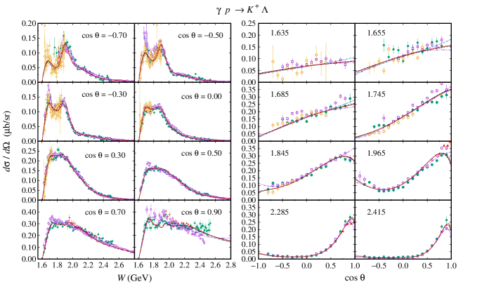
Figure 3: Energy and angular distributions of the $\gamma p\to K^{+}\Lambda$ differential cross section obtained in the present work and from the latest experimental data. Data shown in this figure are taken from the LEPS 2006 (solid triangles Sumihama06 ), CLAS 2006 (solid squares Bradford:2005pt ), CLAS 2010 (solid circles mcCracken ), and Crystal Ball 2014 (open circles Jude:2013jzs ) collaborations. For notation of the curves see Fig. 4.

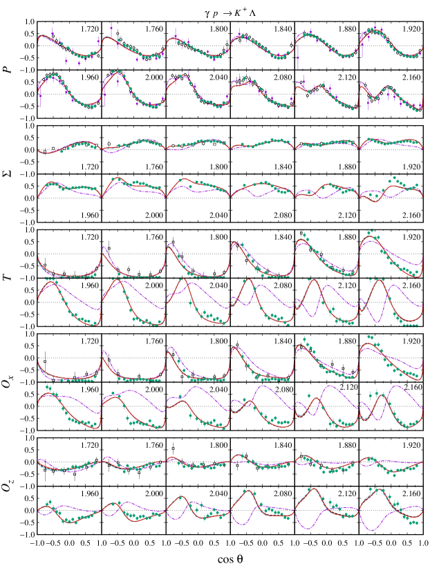
Figure 4: Angular distributions of the recoil polarization $P$, photon asymmetry $\Sigma$, target asymmetry $T$, and photon-recoil double polarizations $O_{x}$ and $O_{z}$ for the $\gamma p\to K^{+}\Lambda$ process obtained from the previous multipole model (dot-dashed curves Mart:2017mwj ), the original field theoretic model involving the nucleon resonances with spins up to 9/2 (dashed curves Clymton:2017nvp ), and the present work (solid curves). The experimental data shown in this figure are taken from the GRAAL 2007 (open squares lleres:2007 ), CLAS 2006 (solid squares Bradford:2005pt ), CLAS 2010 (open circles mcCracken ), and CLAS 2016 (solid circles paterson ) collaborations.

For the recoil polarization $P$ shown in Fig. 4 all models can nicely reproduce the new and older data. This is not surprising because the recoil polarization data have been available since the last decades, whereas the new CLAS 2016 data paterson are consistent with the older ones. The same result is also shown by the photon $\Sigma$ and target $T$ asymmetries, where we can see that our previous multipole model Mart:2017mwj (shown by the dot-dashed curves in Fig. 4) can easily fit the low energy data but fails to reproduce the higher energy ones, since it was fitted to the the GRAAL 2007 data lleres:2007 which are available for $W$ only up to 1.9 GeV. A similar situation also occurs in the case of double polarizations $O_{x}$ and $O_{z}$.

In summary, our present models can nicely reproduce experimental data for the $\gamma p\to K^{+}\Lambda$ channel. This is expected because the difference between the models originates from the $\gamma n\to K^{0}\Lambda$ channel. Pictorially, the former is illustrated in the upper panel of Fig. 5, where we can see that only the model M0 slightly differs from the other models. We have discussed the reason behind this phenomenon; i.e., the corresponding differential cross section is slightly larger for $W<1.9$ GeV but turns out to be smaller as $W\gtrsim 1.9$ GeV.

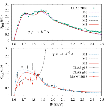
Figure 5: As in Fig. 2 but for the previous Clymton:2017nvp (M0) and present (M1$-$M3) analyses. Note that the previous analysis Clymton:2017nvp did not predict the $\gamma n\to K^{0}\Lambda$ total cross section.

The situation is very different in the case of the $\gamma n\to K^{0}\Lambda$ channel. As shown in the bottom panel of Fig. 5 the inclusion of MAMI data (model M2) results in a divergent total cross section for $W\gtrsim 1.9$ GeV, in contrast to the other models. Obviously this result is caused by the MAMI data, which are limited only up to 1.855 GeV. Above this energy region there is practically no constraint for the $\gamma n\to K^{0}\Lambda$ cross section. By adding the CLAS data to this result we obtain model M3 which nicely reproduces all data for $W>1.8$ GeV and yields a compromise total cross section for $W<1.8$ GeV.

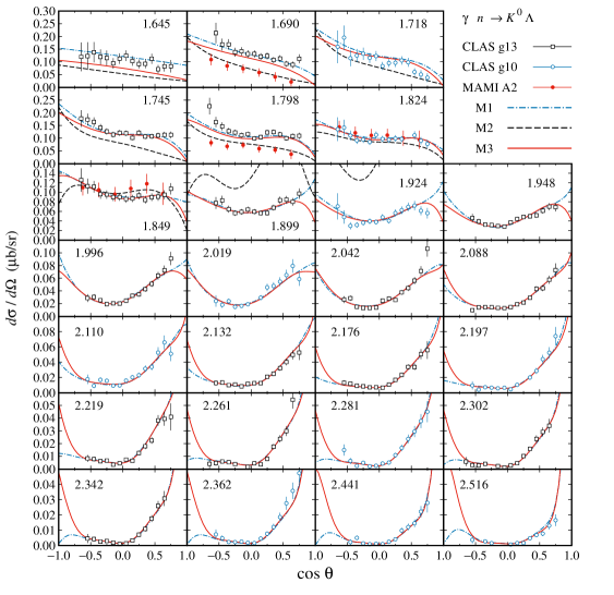
Figure 6: As in the bottom panel of Fig. 5, but for the angular distribution of $\gamma n\to K^{0}\Lambda$ differential cross section.

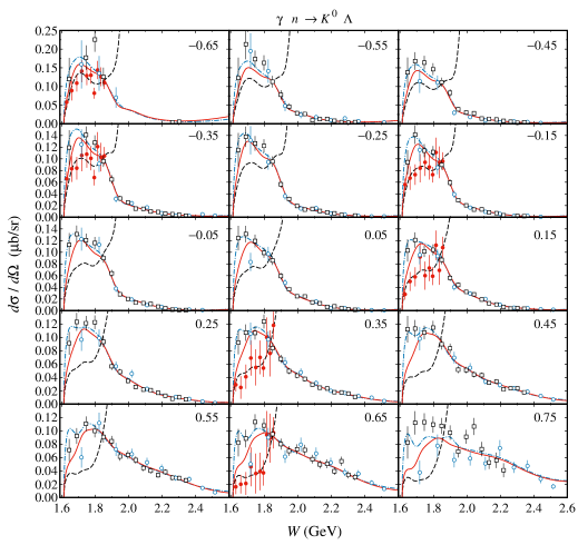
Figure 7: As in Fig. 6, but for the energy distribution.

The angular and energy distributions of the differential cross section shown in Figs. 6 and 7, respectively, reveal more information. Whereas the difference between models M1 and M2 is clear, the difference between models M1 and M3 is observed only in the backward region and, for certain energies, in the forward region (see Fig. 6). It is well known that this behavior originates from the $t$- and $u$-channel contributions that are different for models M1 and M3 as we can see from the corresponding values of $r_{K_{1}K\gamma}$ in Table 4 and $G^{(i)}_{Y^{*}}$ of Table 6. From the energy distribution of the differential cross section shown in Fig. 7 we can understand that the problem of data discrepancy is very clear in the forward direction, where even the CLAS g10 and g13 data show variance for $\cos\theta=0.75$. In the future we expect that experimental measurement of kaon photoproduction should focus on the forward region in order to reconcile this discrepancy as well as to resolve the same problem in the case of the $K^{+}\Lambda$ photoproduction (see, e.g., Ref. Mart:2017mwj ).

III.3 Beam-target helicity asymmetry $E$ in the $\gamma n\to K^{0}\Lambda$ photoproduction

Recently, the CLAS collaboration Ho:2018riy has measured the beam-target helicity asymmetry $E$ in the $\gamma n\to K^{0}\Lambda$ process by using the CEBAF Large Acceptance Spectrometer on a 5-cm-long solid hydrogen deuteride target with the c.m. energy $W$ from 1.70 to 2.34 GeV. Due to the small cross section of the $K^{0}\Lambda$ final state and to detector inefficiencies the corresponding angular and energy bins are very large. The result is given in two energy bins, i.e., from 1.70 to 2.02 GeV and from 2.02 to 2.34 GeV. As shown in Fig. 8 each energy bin contains three data points. Nevertheless, since data on $K^{0}\Lambda$ photoproduction are very limited, these six data points are still invaluable for our present work. However, due to their large error bars we did not include these data in the fitting database. Furthermore, during the fitting process these six data points could not compete with other data that have much smaller error bars, unless a weighting factor was introduced. Therefore, in the present work we only compare the predictions of the three proposed models with these data. For the first energy bin we have calculated the asymmetry $E$ from 1.70 to 2.02 GeV with energy step 10 MeV and compared the 33 calculated asymmetries with experimental data in panels a, b, and c of Fig. 8. We have repeated the calculation for the second energy bin and compared the result with data in panels d, e, and f of Fig. 8. From all panels of Fig. 8 we may conclude that the present work provides the asymmetry bands that are comparable with the experimental data for both energy bins.

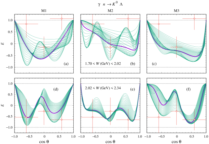
Figure 8: Angular distributions of the $\gamma n\to K^{0}\Lambda$ helicity asymmetry $E$ for two different energy bins. Experimental data are taken from Ref. Ho:2018riy . Thin solid curves are predictions of models M1$-$M3 calculated with 10 MeV energy step and $W$ from 1.70 to 2.02 GeV (from 2.02 to 2.34 GeV) in the panels (a)$-$(c) [(d)$-$(f)]. Thick solid curves are obtained by using the middle values of the energy bins.

By considering the existing error bars shown in Fig. 8 we might conclude that the six available data points are still compatible with all models. However, although their uncertainties are relatively large, these data still exhibit a clear trend. For the low energy bin (from 1.70 to 2.02 GeV) they show a minimum at $\cos\theta=0$. This is in contrast to the high energy bin (from 2.02 to 2.34 GeV), for which the asymmetry is maximum at $\cos\theta=0$. Thus, by comparing the results obtained from models M1 [panels (a) and (d)] and M2 [panels (b) and (e)] we can see that model M1 is more consistent with the data. Panel (e) shows that model M2 predicts a minimum helicity asymmetry near $\cos\theta=0$, in contrast to the experimental data. Perhaps this is not surprising, because model M1 was fitted to the CLAS $\gamma n\to K^{0}\Lambda$ differential cross section, whereas model M2 was fitted to the MAMI data. As expected, the use of both data sets yields a compromise model M3. However, from panels (c) and (f) we can see that model M3 has s relatively similar trend to model M1. We believe that this occurs because in our fitting database the number of CLAS $\gamma n\to K^{0}\Lambda$ differential cross section data is much larger than the MAMI ones and as a consequence the latter have smaller influence.

To conclude this subsection we may safely say that the models that fit the CLAS $\gamma n\to K^{0}\Lambda$ data are more consistent with the presently available helicity asymmetry $E$ data measured by the CLAS collaboration. Nevertheless, more accurate experimental data are strongly required to support this conclusion.

III.4 The significance of individual resonances

As in the previous analyses Mart:2006dk ; Mart:2017mwj in the present work we also investigate the significance of each resonance used in the models by defining the parameter

$$\Delta\chi^{2}~{}=~{}\frac{\chi^{2}_{{\rm All}-N^{*}}-\chi^{2}_{\rm All}}{\chi^{2}_{\rm All}}\times 100\,\%~{},$$ (37)

where $\chi^{2}_{\rm All}$ is the $\chi^{2}$ obtained if all nucleon resonances were used and $\chi^{2}_{{\rm All}-N^{*}}$ is the $\chi^{2}$ obtained if a specific nucleon resonance was excluded. Therefore, Eq. (37) does not express the contribution of the specific resonance in the process, but it solely quantifies how difficult to reproduce experimental data without this resonance. This is the reason why we call it the significance of the resonance. As a further note, in our experience, although Eq. (37) seems to be very simple, the numerical calculations to obtain the $\Delta\chi^{2}$ for each resonance in all models requires high CPU time.

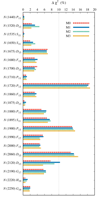
Figure 9: The significance of individual resonances calculated from Eq. (37) for all models investigated in the present work.

The result of previous investigation by using a multipole approach is relatively unstable to the choice of data sets included in the fitting database Mart:2006dk . For instance, the $N(1650)S_{11}$ resonance was found to be very important if we used the SAPHIR data Tran:1998 ; Glander:2003jw , but it turned out to be unimportant if the SAPHIR data were replaced with the CLAS data Bradford:2005pt . The latter would not change if both SAPHIR and CLAS data were used in the fitting process Mart:2006dk . Nevertheless, in this multipole analysis a number of nucleon resonances were found to be important and relatively stable to the choice of data sets. Included in this category are the $N(1720)P_{13}$, $N(1900)P_{13}$, and $N(2080)D_{13}$ resonances. Note that in the recent PDG listing the $N(2080)D_{13}$ state does not exist any longer, it has been replaced by the $N(1875)D_{13}$ state pdg . Therefore, comparing the result for this resonance to the present work is not possible. Moreover, the number of experimental data used in this multipole approach is less than 2500, i.e., much smaller than that used in the present work.

In a more recent multipole analysis, by using the same experimental data points as in model M0 of the present work, it was found that the most significant nucleon resonances in the $K^{+}\Lambda$ photoproduction are the $N(1650)S_{11}$, $N(1720)P_{13}$, $N(1900)P_{13}$, and $N(2060)D_{15}$ states Mart:2017mwj . Thus, we believe that the result of this analysis is more conclusive than that of the previous one Mart:2006dk , especially because the resonance properties were constrained within the uncertainties of PDG estimate as in the present work.

The result of our present work is depicted in Fig. 9, where the significance of each resonance is calculated for all four models. Obviously, our present calculation is stable to the choice of the $K^{0}\Lambda$ data sets, in contrast to the result of previous study Mart:2006dk . From Fig. 9 we might say that the three most important resonances are the $N(1720)P_{13}$, $N(1900)P_{13}$, and $N(2060)D_{15}$ ones. Thus, our present calculation corroborates the finding of our recent multipole analysis Mart:2017mwj , except for the $N(1650)S_{11}$ state. We note that, although the $N(1650)S_{11}$ resonance is insignificant in all models, this resonance still gives sizable contribution to both $K^{+}\Lambda$ and $K^{0}\Lambda$ channels. This can be seen from either the $\Delta\chi^{2}$ shown in Fig. 9 or the coupling constant $G^{(1)}_{N(1650)}$ given in Table 5.

The well-known $N(1710)P_{11}$ resonance is found to be insignificant in the present work. This finding corroborates the result of previous works Mart:2006dk ; Mart:2017mwj . This result is however different from the PDG estimate that rates this resonance with four-star status and branching ratio $\Gamma(\Lambda K)/\Gamma_{\rm total}$ of up to 25% pdg . However, in the present work this is not bad news since with the absence of the important $P_{11}$ state near the threshold we could expect the increase of the probability to find the $P_{11}$ narrow resonance in this energy region. We discuss this topic in the following subsection.

III.5 Narrow resonance in the $K^{0}\Lambda$ photoproduction

The existence of the $J^{p}=1/2^{+}$ ($P_{11}$) narrow resonance has drawn much attention from the hadronic physics communities since it was predicted by the chiral quark soliton model as one of the ten members of the antidecuplet baryons diakonov . These baryons are very interesting because three of them are exotic; i.e., their quantum numbers can only be constructed from five quarks or a pentaquark. The resonance was originally assigned to the $N(1710)P_{11}$ state with the estimated width $\Gamma=41$ MeV, since information from PDG was uncertain pdg_old . However, after the reports of experimental observation of the exotic baryons $\Xi_{3/2}$ NA49 and $\Theta^{+}$ nakano , Ref. Walliser:2003dy found that the $P_{11}$ mass should be either 1650 or 1660 MeV, depending on whether the symmetry breaker $\Delta$ was included or not, respectively. On the other hand, by using the masses of the two exotic baryons as inputs, the authors of Ref. diakonov reevaluated their prediction and found that the $P_{11}$ mass became either 1690 or 1647 MeV, if the mixing with the lower-lying nucleonlike octet was considered or not, respectively diakonov2004 .

The chiral quark soliton model also predicted a large $\eta N$ branching ratio. As a result, there was considerable interest in reevaluation of the $\eta$ photoproduction at energies around 1700 MeV. It was then reported that a substantial enhancement in the cross section of $\eta$ photoproduction off a free neutron has been observed at $W\approx 1670$ MeV kuznetsov . Two experiments performed later by other collaborations confirmed this finding confirmed . Interestingly, this enhancement is absent or very weak in the case of photoproduction off a proton target.

Another mechanism that can be used to study this narrow resonance is the $\pi N$ scattering and photoproduction, since the chiral quark soliton model also predicted a sizable decay width to this channel. By using a modified partial wave analysis Ref. igor obtained the $P_{11}$ mass from $\pi N$ data. This was achieved by scanning the changes of $\chi^{2}$ (called $\Delta\chi^{2}$) in the range of resonance mass between 1620 and 1760 MeV after including this resonance in the $P_{11}$ partial wave. A relatively large $\Delta\chi^{2}$ was observed at 1680 MeV and a smaller one was found at 1730 MeV. This result was found to be independent of the total width and branching ratio of the resonance.

Motivated by the fact that both $N^{*}\to K\Lambda$ and $N^{*}\to\pi N$ branching ratios are predicted by the chiral quark soliton model diakonov , we have investigated the existence of the narrow resonance in the $\gamma p\to K^{+}\Lambda$ channel by utilizing two isobar models which are able to describe the experimental data from threshold up to $W=1730$ MeV mart-narrow . By analyzing the changes in the total $\chi^{2}$ with the variation of resonance mass from 1620 to 1730 MeV and resonance width from 0.1 to 1 MeV and from 1 to 10 MeV we found that the most promising candidate mass and width of this resonance are 1650 and 5 MeV, respectively mart-narrow . However, there was very small signal found in the total cross section since the effect of this resonance on differential cross section switches from decreasing to increasing as the kaon angle increases. The net result in the total cross section is nearly 0. Interestingly, it was found that the narrow resonance signal originates mostly from the $\Lambda$ recoil polarization data. As a consequence, further measurement of recoil polarization with much smaller error bars is strongly recommended.

Given the fact that the effect of this resonance on the cross section of $\eta$ photoproduction is more substantial in the neutron channel kuznetsov , instead of the proton one, it is obviously important to investigate the effect on the neutron channel of kaon photoproduction, i.e., the $\gamma n\to K^{0}\Lambda$ process. In the previous work mart-narrow we fitted the $\gamma p\to K^{+}\Lambda$ experimental data to obtain the $\chi^{2}$ with fixed resonance mass and width and repeated the fitting process for different mass and width values. For the sake of simplicity, in the present work we consider both resonance mass and width as free parameters. Furthermore, since the resonance contribution to the scattering amplitude in the neutron channel is determined by the product of $g_{\gamma nN^{*}}\,g_{K^{0}\Lambda N^{*}}$, we should also consider this product as a free parameter. However, Eq. (27) immediately tell us that this product is related to the $g_{\gamma pN^{*}}\,g_{K^{+}\Lambda N^{*}}$ by the ratio $r_{N^{*}}$ because $g_{K^{+}\Lambda N^{*}}=g_{K^{0}\Lambda N^{*}}$ from Eq. (21). Therefore, for our purpose it is sufficient to extract the ratio $r_{N^{*}}$ from the fitting process.

Table 7: Properties of the $P_{11}$ narrow resonance extracted in the present work obtained from three different models.

Parameter	M1	M2	M3
$m_{N^{*}}$ (MeV)	$1625$	$1670$	$1648$
$\Gamma_{N^{*}}$ (MeV)	$2$	$20$	$3$
$r_{N^{*}}$	$-10.000$	$-1.997$	$6.696$

The extracted ratios, masses, and widths of the $P_{11}$ narrow resonance obtained from the three different models M1$-$M3 are listed in Table 7. Table 7 reveals the substantially different results obtained from M1 and M2 models, i.e., including the CLAS 2016 (paterson ) or MAMI 2018 Akondi:2018shh data, respectively. Including the CLAS 2016 data yields the smallest ratio. Indeed, the extracted ratio reaches its lower bound. Since the cross section is proportional to the squared amplitude, it is obvious that the model M1 yields a strong signal of narrow resonance in the $\gamma n\to K^{0}\Lambda$ channel. The use of MAMI 2018 data yields a completely different result, where from Table 7 we might expect a much weaker signal in this case. However, the extracted mass and width are the largest for this case. We note that if the MAMI data were used the extracted mass corroborated the finding in $\eta$ photoproduction off a free neutron kuznetsov , i.e., 1670 MeV.

The inclusion of both CLAS and MAMI data (model M3) yields a compromise result, where all extracted parameters fall between those of models M1 and M2, up to the sign of $r_{N^{*}}$. The effect of a different sign of $r_{N^{*}}$ in model M3 is discussed later. Thus, the narrow resonance signal in the cross section is still sufficiently large. We also note that the extracted mass and width in this case are closer to the finding in our previous work which only utilized the $\gamma p\to K^{+}\Lambda$ data, i.e., 1650 and 5 MeV, respectively mart-narrow .

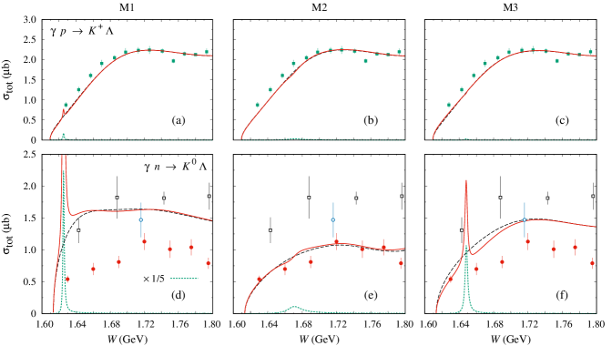
Figure 10: Effects of the $P_{11}$ narrow nucleon resonance on the total cross section of the $\gamma p\to K^{+}\Lambda$ [panels (a)$-$(c)] and $\gamma n\to K^{0}\Lambda$ [panels (d)$-$(f)] channels, obtained from three different models M$-$M3. Solid and dashed curves show the results obtained by including and excluding this resonance in these models, respectively. The dotted curves display contribution of this resonance alone. Experimental data are as in Fig. 5. Note that contribution of the $P_{11}$ narrow resonance in panel d has been rescaled by a factor of 1/5 in order to fit in the same plot.

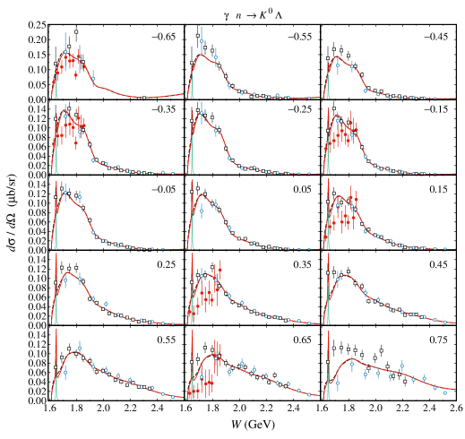
Figure 11: Effects of the $P_{11}$ narrow nucleon resonance on the differential cross section of the $\gamma n\to K^{0}\Lambda$ channel. Solid (dashed) curves are obtained by including (excluding) this resonance in the model M3, respectively. The dotted curves exhibit contribution of this resonance alone. Experimental data are as in Fig. 6.

Comparison between calculated total cross sections for all models and experimental data is shown in Fig. 10. It is obvious that for all models the narrow resonance signal is very weak in the $\gamma p\to K^{+}\Lambda$ channel [panels (a)$-$(c)]. This result corroborates our previous finding obtained by using the same isospin channel mart-narrow . On the contrary, the signal is very strong in the $\gamma n\to K^{0}\Lambda$ channel [see panels (d)$-$(f)]. As expected from the values of $r_{N^{*}}$ given in Table 7 the calculated peak is very strong for model M1 [panel (d)] and very weak for model M2 [panel (e)]. In fact, in the latter the narrow resonance does not create a peak in the total cross section. The effect is very small and presumably cannot be resolved by the current data accuracy.

The use of both CLAS and MAMI data (model M3) reduces the resonance peak in the $\gamma n\to K^{0}\Lambda$ total cross section as shown in panel (f) of Fig. 10. However, different from model M1, where the peak wildly overshoots the data, in model M3 the resonance peak seems to be more natural because the calculated total cross section lies between the CLAS g13 and MAMI data. Incidentally, there is one CLAS g10 datum in this area which can be perfectly reproduced by model M3. Thus, we believe that the model M3 yields a more realistic effect on the cross section.

Different effects of including the narrow resonance in the $\gamma n\to K^{0}\Lambda$ channel appear in the calculated cross section if we compare panels (d) and (f) of Fig. 10. The difference originates from the different sign of the resonance coupling constants, which are represented by the ratios $r_{N^{*}}$ of both models (see Table 7). In panel (d) the effect is directly constructive, whereas in panel (f) the effect is slightly destructive, which is presumably due to the difference phase.

For a further analysis of the narrow resonance effect on the $\gamma n\to K^{0}\Lambda$ process in Fig. 11 we show energy distribution of the differential cross section for a number of kaon scattering angles. From this figure we can understand that the largest effect is obtained in the forward direction. The effect gradually reduces as the kaon angle increases. Therefore, for the investigation of narrow resonance it is important to measure the $\gamma n\to K^{0}\Lambda$ differential cross section in the forward direction with high statistics and $W$ between threshold and 1.70 GeV. Nevertheless, it is also very important to solve the problem of data discrepancy before we can draw a solid conclusion.

IV SUMMARY AND CONCLUSION

We have extended the result of our previous investigation on the $\gamma p\to K^{+}\Lambda$ photoproduction channel to analyze the new $\gamma n\to K^{0}\Lambda$ photoproduction data obtained from the CLAS and MAMI collaborations. To this end, we have used the effective Lagrangian method and coupled the two photoproduction processes by utilizing the isospin symmetry and some information from the Review of Particle Properties of PDG. To analyze more than 9400 experimental data points we have considered a number of parameters in the background and resonance amplitudes as free parameters and adjusted their values by fitting the calculated observables to experimental data. To constrain the resonance parameters we used the uncertainties given in the PDG estimates. The presented models can nicely reproduce the $K^{+}\Lambda$ data and were used to investigate the effects of the data discrepancy found in the $K^{0}\Lambda$ channel. Based on the $K^{0}\Lambda$ data included in the fitting process, i.e., the CLAS, MAMI, or both CLAS and MAMI data sets, three different models M1$-$M3, respectively, were proposed in the present work. All models can nicely reproduce the $K^{+}\Lambda$ data. In the case of the $K^{0}\Lambda$ channel the agreement of model prediction and experimental data depends on the $K^{0}\Lambda$ data set included during the fitting process. However, we found that the new CLAS beam-target helicity asymmetry $E$ for the $\gamma n\to K^{0}\Lambda$ channel can be better explained by the model that fits the $K^{0}\Lambda$ CLAS differential cross section data. We have also scrutinized the significance of each nucleon resonance involved in the models and found that the $N(1720)P_{13}$, $N(1900)P_{13}$, and $N(2060)D_{15}$ resonances are important to reduce the $\chi^{2}$. This result is consistent with the finding of previous works. Finally, we investigated the effect of the $P_{11}$ narrow resonance in both isospin channels and found that the effect is more apparent in the $\gamma n\to K^{0}\Lambda$ process. In this case the model M3 that fits both CLAS and MAMI data yields the most realistic effect. To experimentally investigate the effect of this resonance the present calculation recommends a measurement of the $\gamma n\to K^{0}\Lambda$ differential cross section in the forward direction and with the energy range $W$ from threshold up to 1.70 GeV.

V ACKNOWLEDGMENTS

This work has been supported by the 2019 Q1Q2 Research Grant of Universitas Indonesia, under contract No. NKB-0277/UN2.R3.1/HKP.05.00/2019.

References

- (1) T. Mart and S. Sakinah, Phys. Rev. C 95, 045205 (2017).
- (2) S. Clymton and T. Mart, Phys. Rev. D 96, 054004 (2017).
- (3) T. Mart and A. Sulaksono, Phys. Rev. C 74, 055203 (2006).
- (4) M. Kawaguchi and M. J. Moravcsik, Phys. Rev. 107, 563 (1957).
- (5) G. F. Chew, M. L. Goldberger, F. E. Low, and Y. Nambu, Phys. Rev. 106, 1345 (1957).
- (6) H. Thom, Phys. Rev. 151, 1322 (1966).
- (7) R. A. Adelseck, C. Bennhold, and L. E. Wright, Phys. Rev. C 32, 1681 (1985).
- (8) R. A. Williams, C.-R. Ji, and S. R. Cotanch, Phys. Rev. D 41, 1449 (1990); Phys. Rev. C 43, 452 (1991); 46, 1617 (1992).
- (9) R. A. Adelseck and B. Saghai, Phys. Rev. C 42, 108 (1990).
- (10) M. Bockhorst et al., Z. Phys. C 63, 37 (1994).
- (11) Zhenping Li, Phys. Rev. C 52, 1648 (1995).
- (12) D. Lu, R. H. Landau, and S. C. Phatak, Phys. Rev. C 52, 1662 (1995).
- (13) M. K. Cheoun, B. S. Han, B. G. Yu, and I. T. Cheon, Phys. Rev. C 54, 1811 (1996).
- (14) S. Steininger and U. G. Meissner, Phys. Lett. B 391, 446 (1997).
- (15) M. Q. Tran et al. (SAPHIR Collaboration), Phys. Lett. B 445, 20 (1998).
- (16) T. Mart and C. Bennhold, Phys. Rev. C 61, 012201(R) (1999).
- (17) S. Janssen, J. Ryckebusch, W. Van Nespen, D. Debruyne, and T. Van Cauteren, Eur. Phys. J. A 11, 105 (2001)
- (18) A. Martinez Torres, K. P. Khemchandani, U. G. Meissner, and E. Oset, Eur. Phys. J. A 41, 361 (2009).
- (19) T. Mart and M. J. Kholili, Phys. Rev. C 86, 022201(R) (2012).
- (20) V. A. Nikonov, A. V. Anisovich, E. Klempt, A. V. Sarantsev, and U. Thoma, Phys. Lett. B 662, 245 (2008).
- (21) K. H. Glander et al., Eur. Phys. J. A 19, 251 (2004).
- (22) R. Bradford et al. (CLAS Collaboration), Phys. Rev. C 73, 035202 (2006).
- (23) T. Mart, Phys. Rev. C 62, 038201 (2000).
- (24) A. V. Sarantsev et al., Eur. Phys. J. A 25, 441 (2005).
- (25) M. Sumihama et al. (LEPS Collaboration), Phys. Rev. C 73, 035214 (2006).
- (26) K. Hicks et al., Phys. Rev. C 76, 042201 (2007).
- (27) M. E. McCracken et al. (CLAS Collaboration), Phys. Rev. C 81, 025201 (2010).
- (28) O. V. Maxwell, Phys. Rev. C 85, 034611 (2012); 76, 014621 (2007); A. de la Puente, O. V. Maxwell, and B. A. Raue, Phys. Rev. C 80, 065205 (2009).
- (29) B. Borasoy, P. C. Bruns, U. G. Meissner, and R. Nissler, Eur. Phys. J. A 34, 161 (2007).
- (30) L. De Cruz, T. Vrancx, P. Vancraeyveld, and J. Ryckebusch, Phys. Rev. Lett. 108, 182002 (2012).
- (31) J. Landay, M. Mai, M. Döring, H. Haberzettl, and K. Nakayama, Phys. Rev. D 99, 016001 (2019).
- (32) M. Tanabashi et al. (Particle Data Group), Phys. Rev. D 98 030001 (2018).
- (33) T. Feuster and U. Mosel, Phys. Rev. C 59, 460 (1999).
- (34) V. Shklyar, H. Lenske and U. Mosel, Phys. Rev. C 93, 045206 (2016).
- (35) W. T. Chiang, F. Tabakin, T. S. H. Lee, and B. Saghai, Phys. Lett. B 517, 101 (2001).
- (36) B. Julia-Diaz, B. Saghai, T. S. H. Lee, and F. Tabakin, Phys. Rev. C 73, 055204 (2006).
- (37) H. Kamano, S. X. Nakamura, T.-S. H. Lee, and T. Sato, Phys. Rev. C 88, 035209 (2013).
- (38) A. V. Anisovich, R. Beck, E. Klempt, V. A. Nikonov, A. V. Sarantsev, and U. Thoma, Eur. Phys. J. A 48, 15 (2012).
- (39) R. L. Workman, M. W. Paris, W. J. Briscoe, and I. I. Strakovsky, Phys. Rev. C 86, 015202 (2012).
- (40) D. M. Manley, Int. J. Mod. Phys. A 18, 441 (2003).
- (41) B. C. Hunt and D. M. Manley, Phys. Rev. C 99, 055204 (2019).
- (42) D. Rönchen, M. Döring, and U. G. Meißner, Eur. Phys. J. A 54, 110 (2018).
- (43) L. Tiator, Few Body Syst. 59, 21 (2018).
- (44) N. Compton et al. (CLAS Collaboration), Phys. Rev. C 96, 065201 (2017).
- (45) C. S. Akondi et al. (A2 Collaboration), arXiv:1811.05547 [nucl-ex].
- (46) T. Mart, Phys. Rev. D 83, 094015 (2011); 88, 057501 (2013).
- (47) T. Mart, Phys. Rev. C 87, 042201(R) (2013).
- (48) T. Mart and B. I. S. van der Ventel, Phys. Rev. C 78 014004, (2008); Nucl. Phys. A815, 18 (2009).
- (49) T. Mart, Int. J. Mod. Phys. A 23, 599 (2008); Few-Body Syst. 42, 125 (2008).
- (50) T. Mart and C. Bennhold, Nucl. Phys. A639, 237 (1998).
- (51) T. Mart, C. Bennhold, and C. E. Hyde-Wright, Phys. Rev. C 51, R1074 (1995).
- (52) W. W. Buck, R. Williams, and H. Ito, Phys. Lett. B 351, 24 (1995); H. Ito and F. Gross, Phys. Rev. Lett. 71, 2555 (1993); S. A. Ivashyn and A. Y. Korchin, Eur. Phys. J. C 49, 697 (2007); C. J. Burden, C. D. Roberts and M. J. Thomson, Phys. Lett. B 371, 163 (1996).
- (53) S. H. Kim and H. C. Kim, Phys. Lett. B 786, 156 (2018).
- (54) T. Mart, S. Clymton, and A. J. Arifi, Phys. Rev. D 92, 094019 (2015).
- (55) T. Vrancx, L. De Cruz, J. Ryckebusch, and P. Vancraeyveld, Phys. Rev. C 84, 045201 (2011).
- (56) A. Lleres et al. (GRAAL Collaboration), Eur. Phys. J. A 31, 79 (2007).
- (57) R. Bradford et al., Phys. Rev. C 75, 035205 (2007).
- (58) A. Lleres et al. (GRAAL Collaboration), Eur. Phys. J. A 39, 149 (2009).
- (59) T. C. Jude et al. (Crystal Ball at MAMI Collaboration), Phys. Lett. B 735, 112 (2014).
- (60) C. A. Paterson et al. (CLAS Collaboration), Phys. Rev. C 93, 065201 (2016).
- (61) D. G. Ireland, M. Döring, D. I. Glazier, J. Haidenbauer, M. Mai, R. Murray-Smith, and D. Rönchen, arXiv:1904.07616.
- (62) S. Clymton, M.Sc. Thesis, 2018 (unpublished); S. Clymton and T. Mart, 7th International Conference on Mathematics and Natural Sciences (ITB Bandung, Indonesia, 2018).
- (63) H. Haberzettl, C. Bennhold, T. Mart, and T. Feuster, Phys. Rev. C 58, R40 (1998).
- (64) T. Mart, Phys. Rev. C 82, 025209 (2010).
- (65) T. Mart and A. Rusli, Prog. Theor. Exp. Phys. 2017, 123D04 (2017).
- (66) T. Mart, Prog. Theor. Exp. Phys. 2019, 069101 (2019).
- (67) T. Mart, Phys. Rev. C 83, 048203 (2011).
- (68) G. Knochlein, D. Drechsel, and L. Tiator, Z. Phys. A 352, 327 (1995).
- (69) D. H. Ho et al. (CLAS Collaboration), Phys. Rev. C 98, 045205 (2018)
- (70) D. Diakonov, V. Petrov, and M. Polyakov, Z. Phys. A 359, 305 (1997).
- (71) R. M. Barnett et al. (Particle Data Group), Phys. Rev. D 54, 1 (1996).
- (72) C. Alt et al., Phys. Rev. Lett. 92, 042003 (2004).
- (73) T. Nakano et al., Phys. Rev. Lett. 91, 012002 (2003).
- (74) H. Walliser and V. B. Kopeliovich, J. Exp. Theor. Phys. 97, 433 (2003) [Zh. Eksp. Teor. Fiz. 124, 483 (2003)].
- (75) D. Diakonov and V. Petrov, Phys. Rev. D 69, 094011 (2004).
- (76) V. Kuznetsov et al., Phys. Lett. B 647, 23 (2007).
- (77) F. Miyahara et al., Prog. Theor. Phys. Suppl. 168, 90 (2007); I. Jaegle et al., Phys. Rev. Lett. 100, 252002 (2008).
- (78) R. A. Arndt, Ya. I. Azimov, M. V. Polyakov, I. I. Strakovsky, and R. L. Workman, Phys. Rev. C 69, 035208 (2004).