Covariate Selection for Generalizing Experimental Results:
Application to Large-Scale Development Program in Uganda

Abstract

Generalizing estimates of causal effects from an experiment to a target population is of interest to scientists. However, researchers are usually constrained by available covariate information. Analysts can often collect much fewer variables from population samples than from experimental samples, which has limited applicability of existing approaches that assume rich covariate data from both experimental and population samples. In this article, we examine how to select covariates necessary for generalizing experimental results under such data constraints. In our concrete context of a large-scale development program in Uganda, although more than 40 pre-treatment covariates are available in the experiment, only 8 of them were also measured in a target population. We propose a method to estimate a separating set – a set of variables affecting both the sampling mechanism and treatment effect heterogeneity – and show that the population average treatment effect (PATE) can be identified by adjusting for estimated separating sets. Our algorithm only requires a rich set of covariates in the experimental data, not in the target population, by incorporating researcher-specific constraints on what variables are measured in the population data. Analyzing the development experiment in Uganda, we show that the proposed algorithm can allow for the PATE estimation in situations where conventional methods fail due to data requirements.

Keywords: Causal inference, External validity, Generalization, Randomized experiments

1 Introduction

Over the last few decades, social and biomedical scientists have developed and applied an array of statistical tools to make valid causal inferences [21]. In particular, randomized experiments have become the mainstay for estimating causal effects. Although many scholars agree upon the high internal validity of experimental results, there is a debate about how scientists should infer the impact of policies and interventions on broader populations [19, 3, 20, 4, 13]. This issue of generalizability [37] is pervasive in practice because randomized controlled trials are often conducted on non-representative samples [35, 14, 1, 36].

In this paper, we examine how to generalize the experimental results of the Youth Opportunities Program (YOP) in Uganda, which aims to help the poor and unemployed become self-employed artisans and increase incomes. This large scale development program, involving more than 10,000 individuals was implemented by the government of Uganda and the authors of [6] from 2008 to 2012. Young adults in Northern Uganda were invited to form groups and submit grant proposals for vocational training and to start independent trades. To evaluate the causal impact of the program, funding was randomly assigned and a host of economic variables (e.g., employment and income) were measured.

The question of generalizability is especially important in this application. The aim of such development programs is elegantly noted in [15], “the benefits of knowing which programs work and which do not extend far beyond any program or agency, and credible impact evaluations are global public goods in the sense that they can offer reliable guidance to international organizations, governments, donors, and nongovernmental organizations (NGOs) beyond national borders.” Researchers and policy makers are not just concerned to learn about the very individuals who participated in the trial. The ultimate goal is to learn whether and how much the program can improve economic conditions in a larger target population — about 10 million people in Northern Uganda [16].

Despite its importance, estimating population average treatment effects is not straightforward because we have to adjust for differences between experimental samples and the target population. One pervasive question is what covariates should and can we adjust for? Although previous research shows that adjusting for a set of variables explaining sampling mechanism or treatment heterogeneity is sufficient for generalization [37, 5], researchers are often constrained by available covariate information in applied settings.

In this paper, we address this problem of covariate selection for estimating population average treatment effects. In particular, we develop a data-driven method to estimate a separating set – a set of variables affecting both sampling mechanism and treatment effect heterogeneity. Recent papers show that the population average treatment effect can be identified by adjusting for this separating set [9, 38, 30, 22]. In Section 3, we extend this result and show that the separating set relaxes data requirements of conventional methods by generalizing two widely-used covariate selection approaches: (1) a sampling set – a set of variables explaining how units are sampled into a given experiment [31, 44, 7] and (2) a heterogeneity set: a set of variables explaining treatment effect heterogeneity [22, 29].

In Section 4, we demonstrate that such separating sets are estimable from the experimental data and provide a new estimation algorithm based on Markov random fields. This algorithm only requires that a sampling set be observed in the experimental sample, not in the target population. We estimate a separating set as a set that makes a sampling set conditionally independent of observed outcomes in the experimental data. Therefore, in contrast to conventional methods, we can exploit all covariates in the experiment to find necessary separating sets, even when there are few variables measured in both the experimental and population data.

Importantly, our proposed approach maintains a widely used assumption that a sampling set is observed in the experimental data. However, unlike many existing methods, we do not assume that a sampling set is also observed in the population data. This distinction in data requirement is subtle and yet practically essential because in many applied contexts, a larger number of covariates are measured in the experimental data than in the population data. For example, the experimental data of [6] contains about 40 pre-treatment covariates, even though only 8 of them are also measured in the target population. To estimate separating sets, our proposed method incorporates such user-constraints on what variables can feasibly be collected in the target population. For instance, suppose people selected into the YOP due to social connections, which were unmeasured in the target population. Even in this scenario where conventional methods fail, the proposed method can estimate separating sets accounting for this data constraint, if any exist.

Our article builds on a growing literature on the population average treatment effect, which has two general directions. First, many previous studies have focused on articulating identification assumptions and proposing consistent estimators of the population average treatment effect [37, 44, 7, e.g.,]. In particular, recent papers explicitly show that researchers have to jointly consider treatment effect heterogeneity and the sampling mechanism [9, 38, 30, 22]. These existing approaches often assume researchers have access to a large number of covariates in both the experimental sample and the non-experimental target population. In contrast, we provide a new data-driven covariate selection algorithm to find separating sets in situations where researchers have data constraints in the target population. Our focus on covariate selection is similar to recent influential work on causal directed acyclic graphs (causal DAGs) [5, 4]. We differ from the DAG-based approaches in that we empirically estimate separating sets under assumptions about sampling and heterogeneity sets rather than analytically selecting separating sets from fully specified causal DAGs. Although assumptions about the entire causal DAGs are sufficient for covariate selection, the proposed algorithm can estimate separating sets under weaker assumptions about sampling and heterogeneity sets at the expense of statistical uncertainty.

Research in the second direction argues that the necessary assumptions for existing methods are often too strong in practice. Recent papers have explored methods for sensitivity analyses [2, e.g.,] and bounds [8, e.g.,] to achieve partial identification under weaker assumptions. In particular, [29, 28] also consider data scenarios where the experimental data has a richer set of covariates than the target population data, and propose a sensitivity analysis by specifying sensitivity parameters that captures the distribution of covariates unmeasured in the target population data. Our paper is complementary to these approaches. We instead focus on the point identification of the population average treatment effect and alleviate strong assumptions about data requirements by adding an additional step of estimating a separating set. Our approach can also be used in conjunction with sensitivity analysis; the proposed method can estimate a smaller separating set, thereby reducing the number of unobserved covariates that sensitivity analyses have to consider. We provide further discussions about relationships between our proposed approach and sensitivity analysis in Section 4.4.

2 Youth Opportunities Program in Uganda

As well documented by the World Bank, a large number of young adults in developing countries are unemployed or underemployed [41]. In addition to its direct implication to poverty, concerns for policy makers are that such large young and unemployed populations can increase risk of crime and social unrest [6]. Uganda, especially conflict-affected Northern Uganda, is not an exception. According to estimates from the government, two-thirds of northern Ugandans could not meet basic needs, about 50% were illiterate, and most were underemployed in subsistence agriculture in 2006 [16].

In this paper, we study the Youth Opportunities Program (YOP) in Uganda, designed to help the poor and unemployed become self-employed artisans and increase incomes. This intervention is one example of widely used cash transfer programs in which participants are offered a certain amount of cash in the hope that they invest in training and start new, profitable enterprises. In 2008, the government invited young adults in Northern Uganda to form groups and submit grant proposals for how they would use a grant for vocational training and business start-up. Then, funding was randomly assigned among 535 screened, eligible applicant groups — 265 and 270 groups to treatment and control, respectively. Treatment groups received a one-time unsupervised grant worth $7,500 on average — about $382 per group member, roughly their average annual income. Following the original analysis, we focus on a binary treatment, whether they receive any grants or not through the YOP.

To evaluate the impact of this intervention, [6] surveyed 5 people per group three times over four years, resulting in a panel of 2,598 individuals after removing 79 observations due to missing data. They measured 17 outcome variables across five dimensions — employment (7), income (2), investments (3), business formality (3), and urbanization (2). They find that the effects of the YOP are large across all dimensions. Notably, after two years, the treatment groups were 4.5 times more likely to have vocational training, 2.6 times more likely to engage with a skilled trade and had 16% more hours of employment and 42% higher earnings.

Although it is unambiguous that the YOP had large, persistent positive effects on experimental subjects, it is of great policy interest to empirically investigate how much these experimental estimates are generalizable to a larger population. Estimating population average treatment effects (PATE) can inform which specific development policies governments should scale up. While the focus of the program was on Northern Uganda as a whole, participants of the YOP were inevitably not representative, as in many other development programs. To take into account differences between experimental samples and Northern Uganda’s population, [6] merged their experimental samples with a 2008 population-based household survey, the Northern Uganda Survey (NUS). They adjusted for eight variables shared by experimental and population data; gender, age, urban status, marital status, school attainment, household size, durable assets, and district indicators.

In Table 1, we report estimates based on an inverse probability weighting (IPW) estimator [37] that adjusts for the original eight variables. As a reference, we also report estimates of the average treatment effect within the experimental sample, called the sample average treatment effect (SATE). Estimates of the SATEs and PATEs have roughly the same sign, suggesting that the program will have a positive impact on a variety of outcomes even in the target population. Importantly, this finding, however, rests on an assumption that the original eight variables adjust for all relevant differences between the experimental sample and the target population. Given that the magnitude of the PATE estimates has strong implications for a cost-benefit analysis of these large-scale expensive interventions, it is critical to examine this common methodological challenge of covariate selection for generalizing experimental results.

		Original			Original
	SATE	PATE		SATE	PATE
	estimate	estimate		estimate	estimate
Employment			Investments
Average employment hours	5.13	5.87	Vocational training	0.55	0.51
	(1.22)	(3.25)		(0.03)	(0.07)
Agricultural	-0.01	0.75	Hours of vocational training	349.65	277.18
	(1.02)	(2.01)		(23.61)	(51.21)
Nonagricultural	5.14	5.12	Business assets	426.17	400.31
	(0.92)	(2.62)		(82.79)	(125.19)
Skilled trades only	4.75	2.73
	(0.64)	(1.56)	Business Formality
No employment hours	-0.02	0.00	Maintain records	0.12	0.19
	(0.01)	(0.02)		(0.03)	(0.07)
Any skilled trade	0.27	0.24	Registered	0.06	0.07
	(0.03)	(0.07)		(0.02)	(0.04)
Works mostly in a skilled trade	0.06	-0.01	Pays taxes	0.08	-0.01
	(0.01)	(0.03)		(0.02)	(0.06)
Income			Urbanization
Cash earnings	13.41	12.15	Changed parish	0.01	-0.03
	(3.87)	(5.3)		(0.02)	(0.07)
Durable assets	0.11	0.09	Lives in Urban area	-0.01	-0.06
	(0.05)	(0.16)		(0.03)	(0.07)

Table 1: Estimates of Sample Average Treatment Effects and Population Average Treatment Effects based on the Original Eight Variables. Note: We estimated population average treatment effects (PATE) of the above 17 outcomes using an inverse probability weighting estimator with standard errors clustered by group. Weights are estimated by a logistic regression including the eight variables additively. See details of the estimation in Section 5. As a reference, we also report estimates of the sample average treatment effect (SATE).

In practice, there are several pervasive concerns about covariate selection. First, although it is common to adjust for all observed covariates shared by experimental and population data, it is unclear whether such sets of covariates include all necessary covariates for generalization. In fact, the authors carefully pay attention to this point in the original paper; “young adults are selected into our sample because of unobserved initiative, connections or affinity for entrepreneurship” [6]. If there are unobserved differences between the experimental and population samples, the original PATE estimate would be biased. Second, it is also possible that the original analysis adjusted for unnecessary variables, resulting in inefficient estimators of the PATE. [25] show that weighting on many variables, particularly those not highly correlated to treatment effect heterogeneity, can lead to inefficient estimation of the PATE. In this paper, we investigate necessary and sufficient sets of covariates for generalizing experimental estimates, called separating sets, and then provide a new algorithm to empirically estimate such sets. We select the separating sets under several different assumptions and assess how estimates of the PATE vary. Our reanalysis of this experiment appears in Section 5.

3 Separating Sets For Generalization

This section sets up the potential outcomes framework [27, 32] for studying population average treatment effects. We review a definition of a separating set — a set of variables affecting both the sampling mechanism and treatment effect heterogeneity, and then show that a sampling set and a heterogeneity set, the main focus of existing approaches, are special cases of the separating sets.

3.1 The Setup

We consider a scenario in which we have two data sets. Following [7], we define the first sample of $n$ individuals to be participants in a randomized experiment (“Experimental Data”) and the second data set to be a random sample of $m$ individuals from the target population (“Population Data”). In our application, the experimental data has 2,598 individuals and the population data contains 21,348 individuals. We define a sampling indicator $S_{i}$ taking $1$ if unit $i$ is in the experiment and $0$ if unit $i$ is in the target population. We assume that every unit has non-zero probability of being in the experiment. Although experimental units can be randomly sampled from the target population in ideal settings, units often non-randomly select into the experiment, as in the YOP, making the experimental sample non-representative. Note that we consider cases in which units are either in the experimental data or in the target population data, but similar results hold for cases in which the experimental sample is a subset of the target population.

Let $T_{i}$ be a binary treatment assignment variable for unit $i$ with $T_{i}=1$ for treatment and $0$ for control. We define $Y_{i}(t)$ to be the potential outcome variable of unit $i$ if the unit were to receive the treatment $t$ for $t\in\{0,1\}$. In this paper, we make a stability assumption, which states that there is neither interference between units nor different versions of the treatment, either across units or settings [33, 38, 44]. We define pre-treatment covariates $\mathbf{X}_{i}$ to be any variables not affected by the treatment variable.

We are interested in estimating the average treatment effect in the target population. We call this causal estimand the population average treatment effect (PATE).

Definition 1 (Population Average Treatment Effect).

$$\tau\equiv\mathbb{E}[Y_{i}(1)-Y_{i}(0)\mid S_{i}=0],$$

where $S_{i}=0$ represents the target population data.

The treatment assignment mechanism is controlled by researchers within the experiment ($S_{i}=1$), but it is unknown for units in the target population ($S_{i}=0$; observational data). Formally, we assume that the treatment assignment is randomized within the experiment.

Assumption 1 (Randomization in Experiment).

$$\{Y_{i}(1),Y_{i}(0),\mathbf{X}_{i}\}\ \mbox{$\perp\!\!\!\perp$}\ T_{i}\mid S_{i}=1$$

This assumption holds by design in randomized experiments. Here, we consider unconditional randomization, but results in the paper can be naturally extended to settings with randomization conditional on some pre-treatment covariates. Finally, for each unit in the experimental condition, only one of the potential outcome variables can be observed, and the realized outcome variable for unit $i$ is denoted by $Y_{i}=T_{i}Y_{i}(1)+(1-T_{i})Y_{i}(0)$ [32].

3.2 Definition of Separating Sets and Identification

Recent papers show that the PATE can be identified by a set of variables affecting both treatment effect heterogeneity and the sampling mechanism [9, 38, 30, 22]. In this paper, we refer to this set as a separating set and investigate its statistical properties. Formally, a separating set is any set that makes the sampling indicator and treatment effect heterogeneity conditionally independent.

Definition 2 (Separating Set).

A separating set is a set $\mathbf{W}$ that makes the sampling indicator and treatment effect heterogeneity conditionally independent.

$$Y_{i}(1)-Y_{i}(0)\ \mbox{$\perp\!\!\!\perp$}\ S_{i}\mid\mathbf{W}_{i}.$$ (1)

This definition of a separating set contains two simple cases: (1) when no treatment effect heterogeneity exists and (2) when the experimental sample is randomly drawn from the target population. In both of these cases, $\mathbf{W}_{i}=\{\varnothing\}$. This separating set also encompasses two common approaches in the literature as special cases. First, researchers often employ statistical methods based on a sampling set – a set of all variables affecting the sampling mechanism [37, e.g.,]. Second, researchers might adjust for a heterogeneity set – a set of all variables governing treatment effect heterogeneity [22, e.g.,]. Below, we formalize these sets based on the potential outcomes framework.

We define a sampling set as a set of variables that determines the sampling mechanism by which individuals come to be in the experimental sample. For example, when a researcher implements stratified sampling based on gender and age, the sampling set consists of those two variables. When researchers control the sampling mechanism, a sampling set is known by design. However, when samples are selected without such an explicit sampling design, a sampling set is unknown and in practice, researchers must posit a sampling mechanism. For example, [6] assume that a sampling set consists of eight variables: gender, age, urban status, marital status, school attainment, household size, durable assets, and district indicators.

Formally, we can define a sampling set $\mathbf{X}^{S}$ as follows.

Definition 3 (Sampling Set).

$$\{Y_{i}(1),Y_{i}(0),\mathbf{X}_{i}^{-S}\}\ \mbox{$\perp\!\!\!\perp$}\ S_{i}\mid\mathbf{X}_{i}^{S}$$ (2)

where $\mathbf{X}^{-S}$ is a set of pre-treatment variables that are not in $\mathbf{X}^{S}$.

This conditional independence means that the sampling set is a set that sufficiently explains the sampling mechanism. Given the sampling set, the sampling indicator is independent of the joint distribution of potential outcomes and all other pre-treatment covariates. We refer to variables in the sampling set as sampling variables.

The other popular approach is to adjust for a set of all variables explaining treatment effect heterogeneity, which we call a heterogeneity set. Formally, we can define a heterogeneity set $\mathbf{X}^{H}$ as follows.

Definition 4 (Heterogeneity Set).

$$Y_{i}(1)-Y_{i}(0)\ \mbox{$\perp\!\!\!\perp$}\ \{S_{i},\mathbf{X}_{i}^{-H}\}\mid\mathbf{X}_{i}^{H},$$ (3)

where $\mathbf{X}^{-H}$ is a set of pre-treatment variables that are not in $\mathbf{X}^{H}$.

In this case, because a heterogeneity set fully accounts for treatment heterogeneity, $Y_{i}(1)-Y_{i}(0)$ is independent of all other variables. We refer to variables in the heterogeneity set as heterogeneity variables. In our application, [6] discuss at least two heterogeneity variables, gender and initial credit constraints.

We want to emphasize that a sampling set and a heterogeneity set are special cases of a separating set in the sense that both sets satisfy equation (1). Yet, there may exist many other separating sets, which we explore in Section 4.

Finally, the PATE is nonparametrically identified by adjusting for a separating set [9, 38, 30, 22].

Result 1 (Identification of the PATE).

The PATE is identified with separating set $\mathbf{W}_{i}$ under Assumption 1.

$$\tau = \int\biggl{\{}\mathbb{E}[Y_{i}\mid T_{i}=1,S_{i}=1,\mathbf{W}_{i}=\mathbf{w}]-\mathbb{E}[Y_{i}\mid T_{i}=0,S_{i}=1,\mathbf{W}_{i}=\mathbf{w}]\biggr{\}}dF_{\mathbf{W}_{i}\mid S_{i}=0}(\mathbf{w}),$$

where $F_{\mathbf{W}_{i}\mid S_{i}=0}(\mathbf{w})$ is the cumulative distribution function of $\mathbf{W}$ conditional on $S_{i}=0$.

As sampling and heterogeneity sets are special cases of a separating set, the PATE is identified with the same formula.

3.2.1 Illustration with A Causal DAG.

We consider a causal DAG in Figure 1 as a concrete illustration based on a selection diagram approach [4]. In this causal DAG, three variables $\{X_{2},X_{4},X_{5}\}$ serve as a sampling set, which has direct arrows to sampling variable $S$. Three variables $\{X_{1},X_{2},X_{3}\}$ serve as a heterogeneity set, which has direct arrows to outcome variable $Y$ and can moderate the causal effect of $T$ on $Y$. Finally, from Definition 2, there are many valid separating sets, including the sampling and heterogeneity sets, but the smallest separating set is $\{X_{2},X_{3}\}$, which makes the sampling indicator $S$ and the outcome variable $Y$ conditionally independent. The key is that there are potentially many valid separating sets, and researchers can use any of them for identification given their data constraint.

Remark 1..

We only use the causal DAG in Figure 1 as an illustrative example, and our proposed approach relies only on assumptions we clarify in Section 4 using the potential outcomes. We do not use any particular causal DAG structure in Figure 1, and we do not assume knowledge of the underlying causal DAG structure. When knowledge of the underlying causal DAG is available, results in the causal diagram literature are of great importance, and we refer readers to [4].

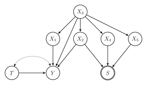
Figure 1: Example of a Causal DAG based on a selection diagram approach [4]. Note: Three variables $\{X_{2},X_{4},X_{5}\}$ serve as a sampling set, three variables $\{X_{1},X_{2},X_{3}\}$ as a heterogeneity set, and two variables as the smallest separating set $\{X_{2},X_{3}\}$.

4 Identification and Estimation of Separating Sets

In this section, we first show that a variant of separating sets, which is sufficient for the identification of the PATE, is estimable even when a sampling set is unobserved in the population data as far as it is observed in the experimental data (Section 4.1). This is in contrast to existing methodologies which assume that a sampling set is observed in both of the experimental and population data. This distinction is subtle and yet practically important because in many applied contexts, including the YOP [6], a larger number of covariates are measured in the experimental data than in the population data. This is because, while analysts of experiments can often control what variables should be measured within the experiment, population data is usually more expensive; collected by other organizations, such as a national-level survey (the NUS in [6]); or otherwise impractical to collect. Thus, our focus is on this type of common research setting where analysts are able to measure more covariates in the experimental data than in the population data.

After demonstrating the identification of separating sets, we propose an algorithm to estimate separating sets using Markov random fields (Section 4.2).

4.1 Identification of Separating Sets

We begin with the identification of an exact separating set and then turn to the identification of a modified separating set under a weaker assumption.

First, we can estimate an exact separating set in settings where both a sampling set and a heterogeneity set are observed in the experimental data. A key feature of this result is that we only require rich covariate information about the experimental units, not the target population units, to discover separating sets, should they exist.

In many applied research contexts, however, the heterogeneity set is not readily available even in the experimental data. The fundamental problem of causal inference states that only one of two potential outcomes are observable, which implies that the causal effect is unobserved at the unit level, and thus so is the heterogeneity set. For example, in our application, although [6] discuss two specific heterogeneity variables (gender and initial credit constraints), it might be unreasonable to assume away the existence of other potential heterogeneity variables.

We therefore develop an additional method to find a variant of a separating set, which we call a marginal separating set, using only knowledge of a sampling set, a commonly employed assumption in the extant literature. We show that a marginal separating set can be discovered when a sampling set is measured in the experimental data, but not in the target population. Although this data requirement might still be stringent in some contexts, it is much weaker than the one necessary for widely-used existing approaches based on sampling sets, which require that sampling set be measured in the population data as well as in the experimental data.

4.1.1 Identification of Exact Separating Sets

We begin with settings in which a sampling set and a heterogeneity set are observed in the experimental sample. In this setting, we can use the experimental data to identify exact separating sets. Although this data requirement is still restrictive, we emphasize that it does not require rich data on the target population.

Setting 1 (Sampling and Heterogeneity Sets are Observed in Experiment).

Sampling set $\mathbf{X}^{S}$ and heterogeneity set $\mathbf{X}^{H}$ are observed in the experiment ($S_{i}=1$).

In this setting, a separating set is estimable as a set that makes the sampling set and the heterogeneity set conditionally independent within the experimental data.

Theorem 1 (Identification of Separating Sets in Experiment).

In Setting 1, consider a set of covariates $\mathbf{W}$, which is a subset of pre-treatment variables. Under Assumption 1,

$$\widetilde{\mathbf{X}_{i}}^{H}\ \mbox{$\perp\!\!\!\perp$}\ \widetilde{\mathbf{X}_{i}}^{S}\mid\mathbf{W}_{i},T_{i},S_{i}=1 \Longrightarrow Y_{i}(1)-Y_{i}(0)\ \mbox{$\perp\!\!\!\perp$}\ S_{i}\mid\mathbf{W}_{i},$$ (4)

where $\widetilde{\mathbf{X}}^{H}$ and $\widetilde{\mathbf{X}}^{S}$ are the set difference $\mathbf{X}^{H}\setminus\mathbf{W}$ and $\mathbf{X}^{S}\setminus\mathbf{W}$, respectively.

We provide the proof in the supplementary material. Theorem 1 states that as long as we can find a set that satisfies the testable conditional independence on the left hand side, the discovered set is guaranteed to be a separating set. That is, we can identify an exact separating set from the experimental data alone. Note that when $\mathbf{X}^{H}$ and $\mathbf{X}^{S}$ share some variables, those variables should always be in $\mathbf{W}$. Using the selected separating set, researchers can identify the PATE based on Result 1.

Intuitively, this theorem can be explained through two conceptual steps. First, because a heterogeneity set $\mathbf{X}^{H}$ fully explains treatment effect heterogeneity $Y(1)-Y(0)$, the sampling indicator $S$ and $Y(1)-Y(0)$ are conditionally dependent only when $S$ and $\mathbf{X}^{H}$ are conditionally dependent. Second, because a sampling set $\mathbf{X}^{S}$ fully explains the sampling indicator $S$, $S$ and $\mathbf{X}^{H}$ are conditionally dependent only when $\mathbf{X}^{S}$ and $\mathbf{X}^{H}$ are conditionally dependent. Taken together, $S$ and $Y(1)-Y(0)$ are conditionally dependent only when $\mathbf{X}^{S}$ and $\mathbf{X}^{H}$ are conditionally dependent.

Example.

Here, we illustrate the general result from Theorem 1 using the causal DAG in Figure 1 as a concrete example. Suppose we are interested in a separating set $\mathbf{W}=\{X_{2},X_{3}\}$, which has the smallest size. Given that heterogeneity set $\mathbf{X}^{H}=\{X_{1},X_{2},X_{3}\}$ and $\mathbf{X}^{S}=\{X_{2},X_{4},X_{5}\}$, we have $\widetilde{\mathbf{X}}^{H}=X_{1}$ and $\widetilde{\mathbf{X}}^{S}=\{X_{4},X_{5}\}.$ Then, as equation (4) suggests, we have $X_{1}\ \mbox{$\perp\!\!\!\perp$}\ \{X_{4},X_{5}\}\mid X_{2},X_{3},T,S=1$ in the causal DAG in Figure 1. More generally, Theorem 1 guarantees that any set that makes the sampling set and the heterogeneity set conditionally independent within the experimental data is a separating set under Assumption 1.

4.1.2 Identification of Marginal Separating Sets

While Theorem 1 allows us to discover separating sets using the experimental data, a key challenge would be to measure both a sampling set and a heterogeneity set in the experimental data. In particular, it is often difficult to measure the heterogeneity set in practice. We show that a modified version of a separating set – a marginal separating set – is estimable from the experimental data under a weaker assumption. We define a marginal separating set as follows.

Definition 5 (Marginal Separating Set).

A marginal separating set is a set $\mathbf{W}$ that makes the sampling indicator and the marginal distributions of potential outcomes conditionally independent.

$$Y_{i}(t)\ \mbox{$\perp\!\!\!\perp$}\ S_{i}\mid\mathbf{W}_{i}\hskip 14.45377pt\mbox{for }t=\{0,1\}.$$ (5)

We refer to this as a marginal separating set since it renders the marginal, not the joint, distribution of potential outcomes conditionally independent of the sampling process.

Now we turn to our final setting researchers may find themselves in – that the sampling set is observed only in the experimental data. Previous work using the sampling set assumes it is measured in both the experimental sample and the target population [9, 38, 44, 7, e.g.,]. Since researchers often have much more control over what data is collected in the experiment, this final setting greatly relaxes the data requirements of the previous literature.

Setting 2 (Sampling Set is Observed in Experiment).

Sampling set $\mathbf{X}^{S}$ is observed in the experimental data ($S_{i}=1$).

Theorem 2 (Identification of Marginal Separating Sets in Experiment).

In Setting 2, consider a set of covariates $\mathbf{W}$, which is a subset of pre-treatment variables. Under Assumption 1,

$$Y_{i}\ \mbox{$\perp\!\!\!\perp$}\ \mathbf{X}_{i}^{S}\mid\mathbf{W}_{i},T_{i},S_{i}=1 \Longrightarrow Y_{i}(t)\ \mbox{$\perp\!\!\!\perp$}\ S_{i}\mid\mathbf{W}_{i}.$$ (6)

We provide the proof in the supplementary material. Theorem 2 states that as long as we can find a set that makes the observed outcome $Y$ conditionally independent of the sampling set within the experimental data, the discovered set is guaranteed to be a marginal separating set. With a large enough sample size, we can find a marginal separating set from the experimental data alone. Intuition behind this theorem is similar to the one used for Theorem 1. Because the sampling set $\mathbf{X}^{S}$ fully explains the sampling indicator $S$, if the sampling indicator $S$ and the potential outcome $Y(t)$ are conditionally dependent, the sampling set $\mathbf{X}^{S}$ and the observed outcome $Y$ are also conditionally dependent. The marginal separating set may be larger than an exact separating set, as it may include covariates that explain the marginal potential outcomes but not treatment effect heterogeneity. Once we have discovered a marginal separating set using the experimental data, we can identify the PATE with this discovered set.

Result 2 (Identification of the PATE with Marginal Separating Sets).

When a marginal separating set $\mathbf{W}$ is observed both in the experimental sample and the target population, the PATE is identified with the marginal separating set $\mathbf{W}$ under Assumption 1.

$$\tau = \int\biggl{\{}\mathbb{E}[Y_{i}\mid T_{i}=1,S_{i}=1,\mathbf{W}_{i}=\mathbf{w}]-\mathbb{E}[Y_{i}\mid T_{i}=0,S_{i}=1,\mathbf{W}_{i}=\mathbf{w}]\biggr{\}}dF_{\mathbf{W}_{i}\mid S_{i}=0}(\mathbf{w}).$$

We omit the proof because it is straightforward from the one of Result 1.

Set to Adjust For	Data Requirements
	Experiment	Target Population
Sampling set	Sampling set	Sampling set
Heterogeneity set	Heterogeneity set	Heterogeneity set
Estimated separating set (Theorem 1 under Setting 1)	$\left\{\vbox to12.0pt{}\begin{tabular}[]{c}Sampling Set\\ Heterogeneity Set\end{tabular}\right.$	User Specified Constraints
Estimated marginal separating set (Theorem 2 under Setting 2)	Sampling set	User Specified Constraints

Table 2: Identifying the PATE under different data requirements. Note: Many previous approaches assume that a sampling set or a heterogeneity set is measured in both the experimental sample and the target population (the first two rows). Our proposed approaches relax data requirements for the target population by introducing an additional step of estimating separating sets.

Finally, in Table 2, we compare existing methods with two proposed approaches. The first two rows show two common existing approaches based on sampling and heterogeneity sets, respectively. Although the identification of the PATE in those settings is straightforward, it requires rich covariate information from the target population data as well as from the experimental sample. Our approach relaxes data requirements for the target population by introducing an additional step of estimating separating sets. In Setting 1 where we observe both a sampling set and a heterogeneity set in the experimental sample, we can identify exact separating sets from the experimental data alone (Theorem 1). Setting 2 only requires observing a sampling set in the experimental sample and we can identify marginal separating sets (Theorem 2). In the next subsection, we introduce an algorithm that can estimate separating sets subject to user specified data constraints in the target population.

4.2 Estimation of Separating Sets

Here, we propose an estimation algorithm to find a marginal separating set. As shown in Theorem 2, the goal is to find a set that makes a sampling set and observed outcomes conditionally independent within the experimental data. We show how to apply Markov random fields (MRFs) to encode conditional independence relationships among observed covariates and then select a separating set. A similar algorithm can be used for finding an exact separating set.

Our estimation algorithm consists of four simple steps. We provide a brief summary here and then describe each step in order. Step 1: specify all variables in sampling set $\mathbf{X}^{S}$ based on domain knowledge, some of which might not be measured in the population data. Step 2: using the experimental data alone, estimate a Markov random field over an outcome, a treatment, the sampling set and observed pre-treatment covariates. Step 3: enumerate all simple paths from $Y$ to $\mathbf{X}^{S}$ in the estimated Markov graph. Step 4: find sets that block all the simple paths from $Y$ to $\mathbf{X}^{S}$ in the estimated Markov graph.

Estimating Markov Random Fields.

Theorem 2 implies that we can find a marginal separating set by estimating a set of variables $\mathbf{W}$ that satisfies the conditional independence, $Y_{i}\ \mbox{$\perp\!\!\!\perp$}\ \mathbf{X}_{i}^{S}\mid\mathbf{W}_{i},T_{i},S=1.$ To estimate this set, we employ a Markov random field (MRF). MRFs are statistical models that encode the conditional independence structure over random variables via graph separation rules. For example, suppose there are three random variables $A,B$ and $C$. Then, $A\mbox{$\perp\!\!\!\perp$}B\mid C$ if there is no path connecting $A$ and $B$ when node $C$ is removed from the graph (i.e., node $C$ separates nodes $A$ and $B$), so-called the global Markov property [45]. We review basic properties of the MRF in the supplementary material (SM-3), and we refer readers to [45] for its comprehensive discussion. Using the general theory of MRFs, the estimation of a separating set can be recast as the problem of finding a set of covariates separating outcome variable $Y$ and a sampling set $\mathbf{X}^{S}$ in an estimated Markov graph. Therefore, we can find a separating set that satisfies the desired conditional independence as far as we can estimate the MRF over $\{Y,T,\mathbf{X}^{S},\mathbf{X}_{0}\}$ within the experimental data where we define $\mathbf{X}_{0}$ to be all pre-treatment variables measured both in the experimental and population data. We define $\mathbf{Z}\equiv\{\mathbf{X}^{S},\mathbf{X}_{0}\}$ to be pre-treatment covariates from which we select a separating set.

Remark 2..

Note that MRFs are used here to estimate conditional independence relationships of observed covariates as an intermediate step of estimating separating sets. Importantly, they are not used to estimate the underlying causal directed acyclic graphs (causal DAGs). As emphasized earlier in the paper, while we used a causal diagram (Figure 1) as an illustration, we only rely on domain knowledge about sampling sets, and we are not taking the causal graphical approach. Such an approach is powerful when knowledge of the full structure of the underlying causal DAG is available, which we do not assume in this paper.

To estimate a MRF, we use a mixed graphical model [42, 18], which allows for both continuous and categorical variables. More concretely, we assume that each node can be modeled as the exponential family distribution using the remaining variables.

$$\Pr(G_{r}\mid G_{-r})=\mbox{exp}\biggl{\{}\alpha_{r}G_{r}+\sum_{h\neq r}\theta_{r,h}G_{r}G_{h}+\varphi(G_{r})-\Phi(G_{-r})\biggr{\}},$$ (7)

where $G_{-r}$ is a set of all random variables in a Markov graph except for variable $G_{r}$, base measure $\varphi(G_{r})$ is given by the chosen exponential family, and $\Phi(G_{-r})$ is the normalization constant. For example, for a Bernoulli distribution, the conditional distribution can be seen as a logistic regression model.

$$\Pr(G_{r}\mid G_{-r})=\cfrac{\mbox{exp}(\alpha_{r}+\sum_{h\neq r}\theta_{r,h}G_{h})}{\mbox{exp}(\alpha_{r}+\sum_{h\neq r}\theta_{r,h}G_{h})+1}.$$ (8)

In general, we model each node using a generalized linear model conditional on the remaining variables. Using this setup, we can estimate the structure of the MRF by estimating parameters $\{\theta_{r,h}\}_{h\neq r}$; $\theta_{r,h}\neq 0$ for variable $G_{h}$ in the neighbors of variable $G_{r}$ and $\theta_{r,h}=0$ otherwise. We estimate each generalized linear model with $\ell_{1}$ penalty to encourage sparsity [24]. Finally, using the AND rule, an edge is estimated to exist between variables $G_{r}$ and $G_{h}$ when $\theta_{r,h}\neq 0$ and $\theta_{h,r}\neq 0.$ Researchers can also use an alternative OR rule (an edge exists when $\theta_{r,h}\neq 0$ or $\theta_{h,r}\neq 0$) and obtain the same theoretical guarantee of graph recovery.

Estimating Separating Sets.

Given the estimated graphical model, we can enumerate many different separating sets. First, we focus on the estimation of a separating set of the smallest size because it often produces more stable weights and thus improves estimation accuracy. It is important to note that this separating set might not be the smallest with respect to the underlying unknown DAG because MRFs don’t encode all conditional independence relationships between variables. It is the smallest size among all separating sets estimable from MRFs.

We estimate this separating set from pre-treatment covariates $\mathbf{Z}$ as an optimization problem. A separating set should block all simple paths between outcome $Y$ and variables in the sampling set $\mathbf{X}^{S}$. Therefore, we first enumerate all simple paths between $Y$ and $\mathbf{X}^{S}$ and then find a minimum set of variables that intersect all paths.

Define $q$ to denote the number of variables in $\mathbf{Z}$. We then define $\mathbf{d}$ to be a $q$-dimensional decision vector with $d_{j}$ taking $1$ if we include the $j$ th variable of $\mathbf{Z}$ into a separating set and taking $0$ otherwise. We use $\mathbf{P}$ to store all simple paths from $Y$ to each variable in $\mathbf{X}^{S}$ where each row is a $q$-dimensional vector and its $j$ th element takes $1$ if the path contains the $j$ th variable. With this setup, the estimation of the separating set of the smallest size is equivalent to the following linear programming problem given the estimated graphical model.

$$\mbox{ min}_{\mathbf{d}}\ \sum_{j=1}^{q}d_{j}\ \ \ \ \ \mbox{s.t., }\mathbf{P}\mathbf{d}\geq\mathbf{1}.$$

where $\mathbf{1}$ is a vector of ones. The constraints above ensure that all simple paths intersect with at least one variable in a selected separating set, and the objective function just counts the total number of variables to be included into a separating set. Therefore, by optimizing this problem, we can find a set of variables with the smallest size that is guaranteed to block all simple paths.

It is important to emphasize that the estimation of the Markov graph is subject to uncertainty as any other statistical methods. In our application, we incorporate uncertainties about set estimation through bootstrap. We also investigate accuracy of the proposed algorithm through simulation studies in the supplementary material. We find that estimators based on estimated separating sets often have similar standard errors to the ones based on the true sampling set. Although our approach introduces an additional estimation step of finding separating sets to relax data requirements, it does not suffer from substantial efficiency loss.

Incorporating Users’ Constraints.

One advantage of our approach is that we can allow the flexibility for researchers to explicitly specify variables that they cannot measure in the target population. This is important in practice because it is often the case that researchers can measure a large number of covariates in the experimental data but they can collect relatively few variables in the target population. We can easily adjust the previous optimization problem to account for this restriction. Define $\mathbf{u}$ to be a $q$-dimensional vector with $u_{j}$ taking $1$ if we want to exclude the $j$ th variable of $\mathbf{Z}$ from a separating set and taking $0$ otherwise. As we define $\mathbf{X}_{0}$ to be those variables observed in both the experimental sample and the target population, $\mathbf{u}$ will place constraints on those covariates in $\mathbf{X}^{S}$ that are unobservable. Then, the optimization problem above changes as follows.

$$\mbox{ min}_{\mathbf{d}}\ \sum_{j=1}^{q}d_{j}\ \ \ \ \ \mbox{ s.t., }\mathbf{P}\mathbf{d}\geq\mathbf{1}\ \mbox{ and }\ \mathbf{u}^{\top}\mathbf{d}=0$$

In practice, it is possible that there exists no separating set, subject to user constraints. In our example, a true separating set could include social connections, which are not measured in the Northern Uganda Survey (the population data). In this case, there is no feasible separating set and our algorithm finds no separating set.

4.3 Estimation of Population Average Treatment Effect

To estimate the PATE with estimated separating sets, we use an inverse probability weighting estimator. First, we estimate a probability of being in the experiment $\Pr(S_{i}=1\mid\mathbf{W}_{i}),$ for example, using a logistic regression [37, 40] with adjustment for the actual target population size [7]. Following [7], we stack the experimental data and the population data, and $S_{i}=1$ ($S_{i}=0$) indicates that unit $i$ belongs to the experimental data (the population data). We can then estimate generalization weights as

$$\pi_{i}=\frac{1}{\Pr(S_{i}=1\mid\mathbf{W}_{i})}\times\frac{\Pr(S_{i}=0\mid\mathbf{W}_{i})}{\Pr(S_{i}=0)},$$ (9)

where a usual inverse probability is adjusted by $\Pr(S_{i}=0|\mathbf{W}_{i})/\Pr(S_{i}=0)$ because the PATE is defined only with the population data, i.e., $\mathbb{E}[Y_{i}(1)-Y_{i}(0)|S_{i}=0]$. Finally, we compute the inverse probability weighting estimator [37].

$$\hat{\tau}\equiv\cfrac{\sum_{i;S_{i}=1}\pi_{i}p_{i}T_{i}Y_{i}}{\sum_{i;S_{i}=1}\pi_{i}p_{i}T_{i}}-\cfrac{\sum_{i;S_{i}=1}\pi_{i}(1-p_{i})(1-T_{i})Y_{i}}{\sum_{i;S_{i}=1}\pi_{i}(1-p_{i})(1-T_{i})},$$ (10)

where $p_{i}\equiv\Pr(T_{i}=1\mid S_{i}=1,\mathbf{W}_{i})$ is known by the experimental design. We prove its consistency in the supplementary material.

Researchers can also employ an outcome-model-based estimator and a doubly robust estimator for the PATE [43, 11]. To maintain the clear comparison with the original analysis that uses a weighting approach, we will focus on the inverse probability weighting estimator (equation (10)) in Section 5, while we also report results from the other two estimators in the supplementary material (SM-4).

4.4 Relationship with Sensitivity Analysis

Here, we want to clarify relationships between our proposed approach and sensitivity analyses for generalization [29, 28, 2, e.g.,]. In particular, our proposed approach can also be used to simplify sensitivity analysis. Sensitivity analysis in general uses some sensitivity parameters to quantify certain aspects of unobserved covariates. For example, [29, 28] propose a sensitivity parameter that captures the distribution of covariates unmeasured in the target population, and [2] introduce a sensitivity parameter to quantify the predictive power of unobserved covariates relative to that of observed covariates. When there is a much richer set of covariates in the experimental data than the target population data — the common scenario and the main focus of our paper, analysts naturally need to specify a large number of sensitivity parameters to account for such potentially many covariates that are not measured in the target population data.

In such scenarios, it is well known that sensitivity parameters become more difficult to interpret, and analysts need to add more parametric assumptions (e.g., additivity) to handle many unobserved variables. Our proposed approach can be used to first find the smallest separating set within the experimental data. Then, researchers do not need to consider all covariates that are unmeasured in the target population data, and they can focus on a potentially much smaller set of covariates estimated as a separating set. Researchers can then use their preferred sensitivity analysis technique to deal with a much smaller set of covariates that are unmeasured in the target population data.

It is also important to clarify the scope of our approach. While we relax a stringent assumption that a sampling set is measured in both experimental and target population data, Theorem 2 still assumes that a sampling set is observed at least in the experimental data. If researchers are worried that a sampling set is not observed even in the experimental data (i.e., not observed in either the experimental or target population data), sensitivity analysis for completely unobserved covariates might be of greater importance.

5 Empirical Analysis

Applying the proposed method, we examine the YOP described in Section 2. Our focus is on a central methodological challenge of covariate selection. In the original analysis, the authors adjusted for all eight variables shared by the experimental and population data. However, as noted in the original paper, it is unknown whether the original eight variables is a separating set necessary for estimating PATEs. To tackle this pervasive concern, we employ the proposed approach and select a separating set under two different assumptions about a sampling set and a heterogeneity set.

First, we incorporate domain knowledge about a heterogeneity set, while we maintain the original assumption about a sampling set. As explained in Section 3, by combining substantive information about a sampling set and a heterogeneity set, we can find a separating set, which can be much smaller than each one of the two. Relying on this smaller separating set, we find that point estimates are similar to estimates based on the original sampling set, but standard errors of the proposed approach are smaller for 14 out of 17 outcomes that the original analysis studied. Incorporating domain knowledge about a heterogeneity set can help us find a smaller set of variables sufficient for the PATE estimation, thereby improving efficiency.

Second, we relax the original assumption about a sampling set — the shared eight variables contain all relevant variables, and we allow for two additional unobserved variables. In the conventional approach based on a sampling set, researchers cannot estimate PATEs under this assumption. In contrast, the proposed approach estimated appropriate separating sets for 12 out of 17 outcomes, and thus, we can estimate the PATE for those 12 outcomes even with the two additional unobserved sampling variables. At the same time, we reveal that estimated PATEs are sensitive to the original assumption about the sampling mechanism for the other 5 outcomes.

The original experiment used clustered randomization, and therefore, we compute clustered standard errors at the group level, which is the level at which treatments were randomly assigned. While we maintain the no interference assumption [33] we made in Section 3.1, which is the standard assumption in the generalization literature, if researchers wish to account for interference within groups, it is important to additionally account for the difference in group structure between the experimental and target population data. Future work is necessary to consider this intersection of interference and generalization literature.

5.1 Incorporating Domain Knowledge on Heterogeneity Set

To begin with, we maintain an assumption about a sampling set in the original analysis, i.e., $\mathbf{X}^{S}=$ {Gender, Age, Urban, Marital status, School attainment,
Household size, Durable assets, District}. Although the original analysis relies only on this knowledge of the sampling set for the PATE estimation, the authors also carefully discuss a heterogeneity set in their paper. In particular, they discuss two variables: gender and initial credit constraints. There are two natural covariates in the experimental data that capture these concepts, Gender and Initial Saving, respectively. Importantly, however, Initial Saving is measured only in the experimental sample and not in the target population data. Thus, $\mathbf{X}^{H}=$ {Gender, Initial Saving} where the square box represents a variable unmeasured in the target population.

In existing approaches, when a subset of heterogeneity variables are unmeasured in the target population as in this case, it is difficult to incorporate such domain knowledge into analysis and researchers often ignore the heterogeneity set altogether. In contrast, our proposed method uses knowledge about the heterogeneity set to estimate an exact separating set, which is potentially smaller than the observed sampling set and thus can increase the estimation accuracy for the PATE estimation. We first estimate a Markov random field over the union of sampling and heterogeneity sets within the experimental data. Then, we select an exact separating set that makes sampling set $\mathbf{X}^{S}$ and heterogeneity set $\mathbf{X}^{H}$ conditionally independent under a constraint that Initial Saving is unmeasured in the population data and cannot be selected. To take into account uncertainties, we estimate Markov random fields and select exact separating sets in each of 1000 bootstrap samples.

Figure 2 reports the results. The left panel (a) shows the proportion of each variable being estimated to be in an exact separating set over 1000 bootstrap samples. As the definition of separating sets (Definition 2) implies, the intersection of sampling and heterogeneity set, Gender, is always selected. In addition, Durable assets and District are selected almost always. Importantly, when we look at the size of estimated exact separating sets (the right panel (b)), it is often much smaller than the original size of eight (the mean size is $4.11$). This means that even when a sampling set is sufficient for estimating the PATE, researchers can find a smaller separating set by incorporating domain knowledge of heterogeneity sets with the proposed approach.

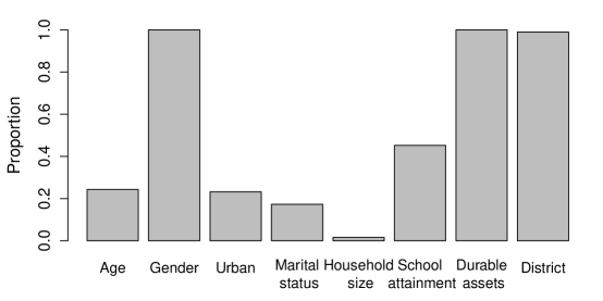
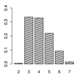
(a) Proportion of Being Estimated as Separating Sets. (b) Size of Estimated Separating Sets.

Figure 2: Estimated Exact Separating Sets. Note: Panel (a) shows the proportion of each variable being estimated to be in an exact separating set over 1000 bootstrap samples. Panel (b) reports the size of estimated exact separating sets over 1000 bootstrap samples.

If assumptions about the sampling set and the heterogeneity set hold, estimators based on the original sampling set $\mathbf{X}^{S}$ and on the estimated separating sets $\mathbf{W}$ are both consistent. However, standard errors of the latter might be smaller because corresponding estimated weights might be more stable.

To estimate the PATEs, we use the inverse probability weighting estimator proposed in Section 4.3. First, we estimate weights using the following logistic regression.

$$\mbox{logit}\{\Pr(S_{i}=1\mid\mathbf{C}_{i})\}=\alpha_{0}+\mathbf{C}_{i}^{\top}\beta,$$ (11)

where $\mathbf{C}=\mathbf{X}^{S}$ for the estimator based on the original sampling set and $\mathbf{C}=\mathbf{W}$ for our proposed estimator. We stack the experimental data (sample size = $2,598$) and the population data (sample size = $21,348$) and $S_{i}=1$ ($S_{i}=0$) indicates that unit $i$ belongs to the experimental data (the population data). We can then estimate weights as $\hat{\pi}_{i}=1/\widehat{\Pr}(S_{i}=1\mid\mathbf{C}_{i})\times\widehat{\Pr}(S_{i}=0\mid\mathbf{C}_{i})/\widehat{\Pr}(S_{i}=0),$ as proposed in Section 4.3. Note that treatment assignment probability in the experiment $\Pr(T_{i}=1\mid S_{i}=1,\mathbf{W}_{i})$ is equal to $\Pr(T_{i}=1\mid S_{i}=1,\mathbf{D}_{i})$ where $\mathbf{D}_{i}$ is a vector indicating 14 districts, because the treatment randomization was stratified by districts [6]. We use the block bootstrap to compute standard errors clustered at the group level as done in the original analysis. To take into account uncertainties of both steps — the estimation of separating sets and that of the PATE, in each of 1000 bootstrap samples, we estimate separating sets, estimate weights, and then estimate the PATE. Note that the difference between the estimator based on the original sampling set and our proposed estimator comes only from the selection of covariates $\mathbf{C}$ in the estimation of weights.

	Original	Sep. Set		Original	Sep. Set
	estimate	estimate		estimate	estimate
Employment			Investments
Average employment hours	5.87	4.79	Vocational training	0.51	0.53
	(3.25)	(2.39)		(0.07)	(0.05)
Agricultural	0.75	0.30	Hours of vocational training	277.18	337.59
	(2.01)	(1.69)		(51.21)	(40.77)
Nonagricultural	5.12	4.49	Business assets	400.31	425.02
	(2.62)	(1.79)		(125.19)	(135.65)
Skilled trades only	2.73	4.36
	(1.56)	(0.99)	Business Formality
No employment hours	0.00	-0.03	Maintain records	0.19	0.20
	(0.02)	(0.03)		(0.07)	(0.07)
Any skilled trade	0.24	0.27	Registered	0.07	0.09
	(0.07)	(0.06)		(0.04)	(0.05)
Works mostly in a skilled trade	-0.01	0.04	Pays taxes	-0.01	0.05
	(0.03)	(0.03)		(0.06)	(0.05)
Income			Urbanization
Cash earnings	12.15	12.54	Changed parish	-0.03	-0.01
	(5.3)	(5.11)		(0.07)	(0.04)
Durable assets	0.09	0.18	Lives in Urban area	-0.06	-0.01
	(0.16)	(0.13)		(0.07)	(0.04)

Table 3: Estimates of Population Average Treatment Effects based on the Original Set and the Estimated Separating Set. Note: We estimated population average treatment effects of 17 outcomes using weights based on the original eight variables (“Original estimate”) and the estimated exact separating set (“Sep. Set estimate”). Standard errors of the proposed estimators are smaller for 14 out of 17 outcomes.

We report results in Table 3. Effects of the YOP are large and positive across many outcomes even among the broader target population. For example, the average employment hours would increase by $4.79$ hours (19% increase compared to the control group), monthly cash earnings would increase by $12,540$ Uganda shilling (36% increase), and a proportion of people enrolled in vocational training would increase by $53$ percentage points (349% increase). Comparing estimates based on the original sampling set and those based on the proposed separating set, we reveal that point estimates are similar to estimates with the original eight variables, and differences between them are not statistically significant at the conventional 0.05 level. This is expected because both estimators are consistent under the assumption that both specified sampling and heterogeneity sets are correct. More interestingly, we find that, for 14 out of 17 outcomes, standard errors of estimators based on the estimated separating sets are smaller than those based on the original sampling set. On average, standard errors of the proposed approach are about 16% smaller. For the outcome “Lives in Urban area,” the standard error reduces more than 45%. This shows that by incorporating domain knowledge about heterogeneity sets, we can estimate smaller separating sets, which often improve efficiency.

5.2 Accounting for Unobserved Sampling Set

In the previous analysis, we maintained the original authors’ assumption about the sampling set and additionally took into account the assumption about the heterogeneity set. Here, we focus on estimating PATEs under weaker assumptions and directly address a concern noted in the original paper that the shared eight variable might not contain all relevant variables. In particular, [6] discuss two potentially problematic variables. First, the authors are concerned that when the government screened applications at the village level, people with more social connections may have received some privilege. Second, people with “affinity for entrepreneurship” [6] might have been more likely to apply for the program in the first place. To account for these two sources of sample selection, we assume that a true sampling set contains two additional variables: (1) Connection, the number of community groups that a respondent belongs to, as a measure of social connections, and (2) Business Advice, total hours spent getting business advice in last 7 days, as a measure of initial motivation and affinity for entrepreneurship. Importantly, both of these two variables are not measured in the population data. Therefore, $\mathbf{X}^{S}=$ {Gender, Age, Urban, Marital status, School attainment, Household size, Durable assets, District, Connection, Business Advice} where the last two variables are measured only in the experiment and not in the population data. Moreover, we don’t make any assumption about heterogeneity sets. Under this assumption, the current practice based on sampling sets or heterogeneity sets cannot estimate any PATEs; weights can be estimated only when sampling sets or heterogeneity sets are measured in both the experimental and population data. In contrast, the proposed method can select appropriate separating sets, should they exist, under such data constraints.

Figure 3: Proportions of Infeasible Solutions. Note: For 17 outcomes, we estimated marginal separating sets under a constraint that two sampling variables are unobserved in the population data. The figure shows the proportion of infeasible solutions for each outcome.

There are two questions of interest for each outcome; (1) Can we find a separating set and estimate the PATE? (2) If we can estimate the PATE, is an estimate different from the one based on the original eight variables? We estimate marginal separating sets using the proposed algorithm. For each outcome $Y$, we first estimate a Markov random field and then select a separating set that makes outcome $Y$ and sampling set $\mathbf{X}^{S}$ conditionally independent under a constraint that the two unobserved variables (Connection, Business Advice) cannot be selected. When the algorithm can find no separating set under the constraint, we call it an “infeasible solution.” We use block bootstrap to compute standard errors clustered at the group level as done in the original analysis. To take into account uncertainties over the covariate selection, we estimate Markov random fields and select separating sets in each of 1000 bootstrap samples.

We begin by computing proportions of infeasible solutions among the 1000 bootstraps (Figure 3). Proportions vary across outcomes, ranging from 0.0% (“Lives in Urban area”) to 26.0% (“Registered”), and on average, 4.70%. Given that the current practice just based on sampling or heterogeneity sets cannot estimate PATEs for any outcomes, it is interesting that the proportions of infeasible solutions are smaller than 5% for 12 out of 17 outcomes. For the remaining five outcomes, the average proportion of infeasible solutions is 11.5%, suggesting that the PATE estimates for these outcomes are sensitive to unobserved sampling variables, Connection and Business Advice.

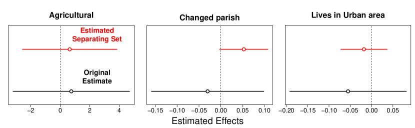
Figure 4: Estimates of Population Average Treatment Effects based on the Original Sets and Estimated Marginal Separating Sets. Note: We estimated population average treatment effects for 3 outcomes that have estimated proportions of infeasible solutions below 1%. Weights are based on the original eight variables (“Original”) and estimated marginal separating sets (“Estimated Separating Set”).

For three outcomes that have less than 1% of infeasible solutions, we also report estimates with 95% confidence intervals in Figure 4. We use the block bootstrap to compute standard errors clustered at the group level. To take into account uncertainties of both steps — the estimation of separating sets and that of the PATE, in each of 1000 bootstrap samples, we estimate separating sets, estimate weights, and then estimate the PATE. We find that point estimates are similar to the original estimates for the two outcomes (“Agricultural” and “Lives in Urban area”), and for “Changed parish,” while point estimates are slightly different due to large standard errors, the difference between the original estimate and the estimate based on an estimated separating set is not statistically significant at the conventional level of $0.05.$ For all three outcomes, standard errors are smaller than the original ones. That is, estimates of the PATEs are robust to alternative separating sets, i.e., even if the sampling set includes additional unobserved variables, substantive conclusions are similar. This result demonstrates that the proposed algorithm of selecting separating sets allows researchers to estimate PATEs in situations where previous methods could not.

6 Concluding Remarks

The increased emphasis on well-identified causal effects in the social and biomedical sciences can sometimes lead researchers to narrow the focus of their research question and limit their findings to the experimental sample. However, primary research questions are often driven by the need to discover the impact of an intervention on a broader population. The extant literature has focused on the mathematical underpinnings concerning the generalizability of experimental evidence. The aim of this paper is to provide applied researchers with a means for uncovering a separating set using the experimental data alone.

Building on previous approaches, we clarify the role of the separating set – and its relationship to the sampling mechanism and treatment effect heterogeneity – in identification of population average treatment effects. It makes clear that there are many possible covariate sets researchers can use for the recovery of population effects, and it allows us to develop a new algorithm that can incorporate researchers’ data constraints on the target population.

As a concrete context, we focus on the YOP in Uganda. For these types of large-scale development programs, potential benefits and necessity of generalization are well known among researchers and policy makers. However, analysts are often constrained by available covariate information, which limits applicability of existing approaches that assume rich covariate data from both the experimental and population samples. Our proposed algorithm can help researchers to estimate appropriate separating sets, if any should exist, even under such data constraints. We find that by incorporating domain knowledge about heterogeneity sets, which is often overlooked in the PATE estimation, we can substantially improve efficiency. We also reveal that the proposed algorithm can find separating sets for 12 out of 17 outcomes, even if we allow for two additional sampling variables that are not measured in the population.

Identifying population effects remains a challenging task for experimental researchers. The results here suggest researchers can increase a chance of generalization by collecting rich covariate information on their experimental subjects, even when their capacity of the population data collection is limited.

Appendix SM-1 Proof of Theorems

Here, we provide proofs for the theorems presented in the paper.

SM-1.1 Proof of Theorem 1

In this proof, we assume that the separating set $\mathbf{W}$ is disjoint with the sampling set $\mathbf{X}^{S}$ and the heterogeneity set $\mathbf{X}^{H}$ for simpler notations. The same proof applies to the case in which some variables of the sampling set or the heterogeneity set are in the separating set. First, we have

$$\mathbf{X}^{H}\ \mbox{$\perp\!\!\!\perp$}\ \mathbf{X}^{S}\mid\mathbf{W},T,S=1.$$ (12)

From Random Treatment Assignment(Assumption 1), we have

$$T\ \mbox{$\perp\!\!\!\perp$}\ \mathbf{X}^{S}\mid\mathbf{W},S=1.$$ (13)

Combining equations (12) and (13) (Contraction in [46]),

$$\{\mathbf{X}^{H},T\}\ \mbox{$\perp\!\!\!\perp$}\ \mathbf{X}^{S}\mid\mathbf{W},S=1,$$

which implies $\mathbf{X}^{H}\ \mbox{$\perp\!\!\!\perp$}\ \mathbf{X}^{S}\mid\mathbf{W},S=1.$ Given that the conditional independence structure of $(\mathbf{X}^{H},\mathbf{X}^{S},\mathbf{W})$ is the same under $S=1$ and $S=0$ (because $S$ only changes the treatment assignment), we have

$$\mathbf{X}^{H}\ \mbox{$\perp\!\!\!\perp$}\ \mathbf{X}^{S}\mid\mathbf{W},S.$$ (14)

From the definition of the sampling variable,

$$\mathbf{X}^{H}\ \mbox{$\perp\!\!\!\perp$}\ S\mid\mathbf{W},\mathbf{X}^{S}.$$ (15)

Combining equations (14) and (15) (Intersection [46]), we have

$$\mathbf{X}^{H}\ \mbox{$\perp\!\!\!\perp$}\ \{S,\mathbf{X}^{S}\}\mid\mathbf{W},$$

which implies

$$\mathbf{X}^{H}\ \mbox{$\perp\!\!\!\perp$}\ S\mid\mathbf{W}.$$ (16)

Additionally, based on the definition of the heterogeneity set,

$$Y(1)-Y(0)\ \mbox{$\perp\!\!\!\perp$}\ S\mid\mathbf{W},\mathbf{X}^{H}.$$ (17)

Therefore, by combining equations (16) and (17) based on Contraction in [46],

$$\{Y(1)-Y(0),\mathbf{X}^{H}\}\ \mbox{$\perp\!\!\!\perp$}\ S\mid\mathbf{W},$$

which implies $Y(1)-Y(0)\ \mbox{$\perp\!\!\!\perp$}\ S\mid\mathbf{W}.$

SM-1.2 Proof of Theorem 2

First, we have

$$Y\ \mbox{$\perp\!\!\!\perp$}\ \mathbf{X}^{S}\mid\mathbf{W},T,S=1.$$ (18)

From Random Treatment Assignment(Assumption 1), we have

$$T\ \mbox{$\perp\!\!\!\perp$}\ \mathbf{X}^{S}\mid\mathbf{W},S=1.$$ (19)

Combining equations (18) and (19) (Contraction in [46]),

$$\{Y,T\}\ \mbox{$\perp\!\!\!\perp$}\ \mathbf{X}^{S}\mid\mathbf{W},S=1,$$

which implies

$$Y(t)\ \mbox{$\perp\!\!\!\perp$}\ \mathbf{X}^{S}\mid\mathbf{W},S=1.$$ (20)

Given that the conditional independence structure of $(Y(1),Y(0),\mathbf{X}^{S},\mathbf{W})$ is the same under $S=1$ and $S=0$ (because $S$ only changes the treatment assignment, relationship for potential outcomes and pre-treatment variables would not change), we have

$$Y(t)\ \mbox{$\perp\!\!\!\perp$}\ \mathbf{X}^{S}\mid\mathbf{W},S,$$ (21)

for $t=\{0,1\}.$

From the definition of the sampling variable, for $t=\{0,1\},$

$$Y(t)\ \mbox{$\perp\!\!\!\perp$}\ S\mid\mathbf{W},\mathbf{X}^{S}.$$ (22)

Combining equations (21) and (22) (Intersection in [46]), we have

$$Y(t)\ \mbox{$\perp\!\!\!\perp$}\ \{S,\mathbf{X}^{S}\}\mid\mathbf{W},$$

which implies

$$Y(t)\ \mbox{$\perp\!\!\!\perp$}\ S\mid\mathbf{W}$$

for $t=\{0,1\}.$ This completes the proof.

Appendix SM-2 IPW Estimator

Here, we show that $\hat{\tau}\xrightarrow{p}\mathbb{E}[Y_{i}(1)-Y_{i}(0)\mid S_{i}=0].$

Proof

First, we rewrite the IPW estimator as follows.

$$\hat{\tau}=\cfrac{\frac{1}{n+m}\sum_{i}S_{i}\pi_{i}p_{i}T_{i}Y_{i}}{\frac{1}{n+m}\sum_{i}S_{i}\pi_{i}p_{i}T_{i}}-\cfrac{\frac{1}{n+m}\sum_{i}S_{i}\pi_{i}(1-p_{i})(1-T_{i})Y_{i}}{\frac{1}{n+m}\sum_{i}S_{i}\pi_{i}(1-p_{i})(1-T_{i})},$$ (23)

where $n$ ($m$) is the sample size of the experimental data (the population data). By the law of large number,

$$\frac{1}{n+m}\sum_{i}S_{i}\pi_{i}p_{i}T_{i}\xrightarrow{p}\mathbb{E}[S_{i}\pi_{i}p_{i}T_{i}] =\mathbb{E}_{\mathbf{W}}\{\pi_{i}\Pr(S_{i}=1\mid\mathbf{W}_{i})p_{i}\Pr(T_{i}=1\mid S_{i}=1,\mathbf{W}_{i})\}$$

$$=\mathbb{E}_{\mathbf{W}}\left\{\frac{\Pr(S_{i}=0\mid\mathbf{W}_{i})}{\Pr(S_{i}=0)}\right\}=1.$$

Similarly, $\frac{1}{n+m}\sum_{i}S_{i}\pi_{i}(1-p_{i})(1-T_{i})\xrightarrow{p}1.$ Again, by the law of large number,

$$\frac{1}{n+m}\sum_{i}S_{i}\pi_{i}p_{i}T_{i}Y_{i}\xrightarrow{p}\mathbb{E}[S_{i}\pi_{i}p_{i}T_{i}Y_{i}],\hskip 7.22743pt\frac{1}{n+m}\sum_{i}S_{i}\pi_{i}(1-p_{i})(1-T_{i})Y_{i}\xrightarrow{p}\mathbb{E}[S_{i}\pi_{i}(1-p_{i})(1-T_{i})Y_{i}].$$

Hence, $\hat{\tau}\xrightarrow{p}\mathbb{E}[S_{i}\pi_{i}p_{i}T_{i}Y_{i}-S_{i}\pi_{i}(1-p_{i})(1-T_{i})Y_{i}].$ We focus on the term on the right.

$$\mathbb{E}\biggl{\{}\pi_{i}\bigg{(}S_{i}p_{i}T_{i}Y_{i}-S_{i}(1-p_{i})(1-T_{i})Y_{i}\bigg{)}\biggr{\}}=\mathbb{E}_{\mathbf{W}}\Biggl{\{}\pi_{i}\mathbb{E}\biggl{\{}S_{i}p_{i}T_{i}Y_{i}-S_{i}(1-p_{i})(1-T_{i})Y_{i}\mid\mathbf{W}_{i}\biggr{\}}\Biggr{\}}$$

$$= \mathbb{E}\Biggl{\{}\pi_{i}\Pr(S_{i}=1\mid\mathbf{W}_{i})\mathbb{E}\biggl{\{}p_{i}T_{i}Y_{i}-(1-p_{i})(1-T_{i})Y_{i}\mid S_{i}=1,\mathbf{W}_{i}\biggr{\}}\Biggr{\}}$$

$$= \mathbb{E}\Biggl{\{}\pi_{i}\Pr(S_{i}=1\mid\mathbf{W}_{i})\{p_{i}\mathbb{E}[T_{i}Y_{i}\mid S_{i}=1,\mathbf{W}_{i}]-(1-p_{i})\mathbb{E}[(1-T_{i})Y_{i}\mid S_{i}=1,\mathbf{W}_{i}]\}\Biggr{\}}$$

$$= \mathbb{E}\Biggl{\{}\pi_{i}\Pr(S_{i}=1\mid\mathbf{W}_{i})\bigg{(}\mathbb{E}[Y_{i}(1)\mid S_{i}=1,\mathbf{W}_{i}]-\mathbb{E}[Y_{i}(0)\mid S_{i}=1,\mathbf{W}_{i}]\bigg{)}\Biggr{\}}$$

$$= \mathbb{E}\Biggl{\{}\pi_{i}\Pr(S_{i}=1\mid\mathbf{W}_{i})\mathbb{E}[Y_{i}(1)-Y_{i}(0)\mid S_{i}=1,\mathbf{W}_{i}]\Biggr{\}}=\mathbb{E}\Biggl{\{}\pi_{i}\Pr(S_{i}=1\mid\mathbf{W}_{i})\mathbb{E}[Y_{i}(1)-Y_{i}(0)\mid S_{i}=0,\mathbf{W}_{i}]\Biggr{\}}$$

$$= \mathbb{E}\Biggl{\{}\frac{\Pr(S_{i}=0\mid\mathbf{W}_{i})}{\Pr(S_{i}=0)}\mathbb{E}[Y_{i}(1)-Y_{i}(0)\mid S_{i}=0,\mathbf{W}_{i}]\Biggr{\}}$$

$$= \int_{\mathbf{W}}\Biggl{\{}\frac{\Pr(S_{i}=0\mid\mathbf{W}_{i})}{\Pr(S_{i}=0)}\mathbb{E}[Y_{i}(1)-Y_{i}(0)\mid S_{i}=0,\mathbf{W}_{i}]\Biggr{\}}p(\mathbf{W})d\mathbf{W}$$

$$= \int_{\mathbf{W}}\mathbb{E}[Y_{i}(1)-Y_{i}(0)\mid S_{i}=0,\mathbf{W}_{i}]p(\mathbf{W}\mid S_{i}=0)d\mathbf{W}=\mathbb{E}[Y_{i}(1)-Y_{i}(0)\mid S_{i}=0],$$

where the first equality follows from the law of conditional expectation given $\mathbf{W}$, the second from the conditional expectation given $S$, the third from the linearity of expectation, the fourth from the conditional expectation given $T$, the fifth from the linearity of expectation, the sixth from the definition of separating $\mathbf{W}$, the seventh from the definition of $\pi,$ the eight from the rule of expectation, the ninth from Bayes rule, and the tenth from the rule of expectation.

Appendix SM-3 Markov Random Fields: Review

A Markov random field (MRF), also known as an undirected graphical model, is a popular statistical model that encodes the conditional independence structure over multiple observed random variables. The main advantage of the MRF is that it encodes the conditional independence relationships of many random variables compactly. While many important results have been derived for MRFs, we focus on one key property, so-called, the global Markov property, which we use in our paper.

MRFs define the conditional independence relationships via simple graph separation rules [45]. For sets of nodes $A$, $B$, and $C$, $A\ \mbox{$\perp\!\!\!\perp$}\ B\mid C$ if and only if there is no path connecting $A$ and $B$ when nodes in $C$ are removed from the graph (i.e., nodes in $C$ separates nodes $A$ and $B$). For example, in Figure SM-5, suppose $A=\{V_{1},V_{2},V_{3}\}$ and $B=\{V_{6},V_{7}\}$. Then, if we define $C=\{V_{4},V_{5}\}$, there is no path connecting $A$ and $B$ once nodes in $C$ are removed from the graph. Therefore, Figure SM-5 encodes the conditional independence relationship, $\{V_{1},V_{2},V_{3}\}\ \mbox{$\perp\!\!\!\perp$}\ \{V_{6},V_{7}\}\mid V_{4},V_{5}$.

As emphasized in the paper, we use the MRF as the statistical model to characterize the conditional independence relationships between observed random variables. We do not use the MRF as a step to estimate the underlying causal DAG.

Figure SM-5: Example of a Markov Random Field (MRF).

Appendix SM-4 Additional Results on Empirical Analysis

In Section 5, we focused on the inverse probability weighting estimator (equation (10)) to maintain the clear comparison with the original analysis that uses the weighting approach. In this section, we report results based on an outcome-model-based estimator and a doubly robust estimator [43]. In particular, for the outcome-model-based estimator, we use a fully-interacted linear model. Within the experimental data, we estimate a linear regression with a specified set of covariates separately for the treatment and control groups. Then, we use the estimated models to predict potential outcomes under treatment and control for the target population data. This outcome-model-based estimator is consistent under the assumption that the outcome model is correctly specified. For the doubly robust estimator, we use an augmented IPW estimator [47, 43] where the outcome model is a fully-interacted linear model and the sampling model is a logistic regression specified in Section 4.3. This doubly robust estimator is consistent if one of the two models — outcome or sampling models — is correctly specified.

We first extend our analyses in Section 5.1. Table SM-4 reports results based on the outcome-model-based estimator (an extension of Table 3). Similarly to the case of the IPW estimator, we find that (1) point estimates based on estimated separating sets are similar to those based on the original sampling set, and (2) standard errors based on our proposed estimated separating sets are smaller for 16 out of 17 outcomes. Table SM-5 reports results based on the doubly robust estimator (an extension of Table 3). Similarly to the cases of the IPW estimator and the outcome-model-based estimator, we find that (1) point estimates based on estimated separating sets are similar to those based on the original sampling set, and (2) standard errors based on our proposed estimated separating sets are smaller for 15 out of 17 outcomes. Therefore, for all three classes of estimators, our proposed approach of using the estimated separating set improves estimation accuracy. Finally, we also compare estimates across three classes of estimators in Table SM-6. Across 17 outcomes, we find that estimates of the PATE are relatively stable across different estimators (none of the differences in estimates are statistically significant at the conventional $0.05$ level), which suggests model misspecification is of little concern.

We next extend our analyses in Section 5.2. Table SM-7 reports results for Section 5.2 by comparing estimates from the outcome-model-based estimator and the doubly robust estimator to estimates from the IPW estimator. While the point estimate for “Agricultural” is unstable due to a relatively large standard error (the first row in Table SM-7), estimates of the PATE are relatively stable across different estimators (none of the differences in estimates are statistically significant at the conventional $0.05$ level), which again suggests model misspecification is of little concern.

	Original		Estimated
	Sampling Set		Separating Set
	Estimate	S.E.	Estimate	S.E.
Average employment hours	4.58	2.35	3.57	1.80
Agricultural	-0.00	1.61	-1.22	1.45
Nonagricultural	4.58	1.77	4.79	1.45
Skilled trades only	3.70	1.03	4.08	0.86
No employment hours	-0.04	0.03	-0.03	0.02
Any skilled trade	0.27	0.05	0.25	0.04
Works mostly in a skilled trade	0.02	0.02	0.04	0.02
Cash earnings	5.20	7.31	8.22	7.02
Durable assets	0.08	0.10	0.06	0.08
Vocational training	0.52	0.05	0.50	0.04
Hours of vocational training	250.32	34.71	280.24	27.43
Business assets	340.79	141.74	367.61	127.23
Maintain records	0.14	0.05	0.14	0.04
Registered	0.03	0.04	0.04	0.03
Pays taxes	0.01	0.05	0.02	0.05
Changed parish	0.04	0.06	-0.02	0.03
Lives in Urban area	-0.01	0.03	-0.01	0.03

Table SM-4: Estimates of the PATEs based on Outcome-Model-Based Estimator, comparing the Original Sampling Set and Estimated Exact Separating Sets. Extension of Table 3 in Section 5.1.

	Original		Estimated
	Sampling Set		Separating Set
	Estimate	S.E.	Estimate	S.E.
Average employment hours	2.49	3.16	2.48	2.73
Agricultural	-2.27	2.73	-2.08	1.83
Nonagricultural	5.10	2.99	4.56	2.24
Skilled trades only	2.29	1.66	3.71	1.14
No employment hours	0.01	0.03	-0.01	0.03
Any skilled trade	0.24	0.07	0.24	0.06
Works mostly in a skilled trade	-0.03	0.03	0.02	0.04
Cash earnings	4.16	8.06	9.02	7.54
Durable assets	0.02	0.15	0.14	0.15
Vocational training	0.49	0.07	0.50	0.05
Hours of vocational training	228.35	50.14	283.26	34.55
Business assets	326.58	178.44	371.18	139.65
Maintain records	0.16	0.07	0.17	0.07
Registered	0.05	0.06	0.06	0.05
Pays taxes	-0.02	0.07	0.01	0.07
Changed parish	0.06	0.07	-0.04	0.05
Lives in Urban area	0.01	0.05	-0.01	0.04

Table SM-5: Estimates of the PATEs based on Doubly Robust Estimator, comparing the Original Sampling Set and Estimated Exact Separating Sets. Extension of Table 3 in Section 5.1.

	IPW		Outcome-Model-based		AIPW
	Estimator		Estimator		Estimator
	Estimate	S.E.	Estimate	S.E.	Estimate	S.E.
Average employment hours	4.79	2.39	3.57	1.80	2.48	2.73
Agricultural	0.30	1.69	-1.22	1.45	-2.08	1.83
Nonagricultural	4.49	1.79	4.79	1.45	4.56	2.24
Skilled trades only	4.36	0.99	4.08	0.86	3.71	1.14
No employment hours	-0.03	0.03	-0.03	0.02	-0.01	0.03
Any skilled trade	0.27	0.06	0.25	0.04	0.24	0.06
Works mostly in a skilled trade	0.04	0.03	0.04	0.02	0.02	0.04
Cash earnings	12.54	5.11	8.22	7.02	9.02	7.54
Durable assets	0.18	0.13	0.06	0.08	0.14	0.15
Vocational training	0.53	0.05	0.50	0.04	0.50	0.05
Hours of vocational training	337.59	40.77	280.24	27.43	283.26	34.55
Business assets	425.02	135.65	367.61	127.23	371.18	139.65
Maintain records	0.20	0.07	0.14	0.04	0.17	0.07
Registered	0.09	0.05	0.04	0.03	0.06	0.05
Pays taxes	0.05	0.05	0.02	0.05	0.01	0.07
Changed parish	-0.01	0.04	-0.02	0.03	-0.04	0.05
Lives in Urban area	-0.01	0.04	-0.01	0.03	-0.01	0.04

Table SM-6: Estimates of the PATEs based on Estimated Exact Separating Sets for Three Estimators. Extension of Section 5.1.

	IPW		Outcome-Model-based		AIPW
	Estimator		Estimator		Estimator
	Estimate	S.E.	Estimate	S.E.	Estimate	S.E.
Agricultural	0.64	1.63	-1.10	1.31	-1.32	1.56
Changed parish	0.05	0.03	0.03	0.03	0.04	0.03
Lives in Urban area	-0.02	0.03	-0.02	0.03	-0.01	0.04

Table SM-7: Estimates of the PATEs based on Estimated Marginal Separating Sets for Three Estimators. Extension of Section 5.2.

Appendix SM-5 Simulation Studies

We turn now to simulations to explore how well the proposed algorithm can recover the PATE. We first verify that our proposed algorithm can obtain a consistent estimator of the PATE. More importantly, we find that estimators based on estimated separating sets often have similar standard errors to the ones based on the true sampling set. Although our approach introduces an additional estimation step of finding separating sets to relax data requirements for the target population, it does not suffer from substantial efficiency loss. Both results hold with and without user constraints on what variables can be measured in the target population.

SM-5.1 Simulation Design

In this subsection, we articulate our simulation design step by step. See the supplementary material for all the details on the simulation design.

Pre-treatment Covariates and Potential Outcome Model.

To consider different types of separating sets, we assume the causal directed acyclic graph (DAG) in Figure SM-6 that encodes causal relationships among the outcome, the sampling indicator, and pre-treatment covariates. In this DAG, there are three conceptually distinct sets that we consider – (1) a sampling set, $X4$ and $X5$, depicted in green, (2) a heterogeneity set, $X2$ and $X3$, depicted in orange, and (3) the minimum separating set, $X1$, highlighted in purple. Three root nodes $X1$, $X6$, $X7$ are normally distributed and other pre-treatment covariates are linear functions of their parents in the DAG. In particular, pre-treatment covariates are generated as follows.

$$X1 \sim\mathcal{N}(0,1)$$

$$X2 =0.7\times X1+\sqrt{1-0.7^{2}}\times\epsilon_{2}$$

$$X3 =0.7\times X1+\sqrt{1-0.7^{2}}\times\epsilon_{3}$$

$$X4 =0.7\times X1+\sqrt{1-0.7^{2}}\times\epsilon_{4}$$

$$X5 =0.3\times X9+\sqrt{1-0.3^{2}}\times\epsilon_{5}$$

$$X6 \sim\mathcal{N}(0,1)$$

$$X7 \sim\mathcal{N}(0,1)$$

$$X8 =-0.7\times X2+\sqrt{1-0.7^{2}}\times\epsilon_{8}$$

$$X9 =0.6\times X1+\sqrt{1-0.6^{2}}\times\epsilon_{9}$$

where $\epsilon_{2},\epsilon_{3},\epsilon_{4},\epsilon_{5},\epsilon_{8},\epsilon_{9}$ are drawn independently and identically from a standard normal distribution, $\mathcal{N}(0,1).$ This results in the following correlation structure for variables $X1-X9$.

$$cor(\textbf{X}) =\begin{pmatrix}1.00&-0.70&0.70&0.70&-0.20&0.00&0.00&0.50&-0.70\\ -0.70&1.00&-0.50&-0.50&0.15&0.00&0.00&-0.70&0.50\\ 0.70&-0.50&1.00&0.50&-0.15&0.00&0.00&0.33&-0.50\\ 0.70&-0.50&0.50&1.00&-0.15&0.00&0.00&0.33&-0.50\\ -0.21&0.15&-0.15&-0.15&1.00&0.00&0.00&-0.10&0.30\\ 0.00&0.00&0.00&0.00&0.00&1.00&0.00&0.00&0.00\\ 0.00&0.00&0.00&0.00&0.00&0.00&1.00&0.00&0.00\\ 0.50&-0.70&0.33&0.33&-0.10&0.00&0.00&1.00&-0.33\\ -0.70&0.50&-0.50&-0.50&0.30&0.00&0.00&-0.33&1.00\end{pmatrix}$$

We then draw the potential outcomes as follows.

$$Y_{i}(T_{i})=5T_{i}+10\times X_{3i}\times T_{i}-10\times X_{2i}\times T_{i}+X_{6i}-3\times X_{8i}+\epsilon_{i}$$

where $\epsilon_{i}\sim N(0,1)$. Thus, the true PATE is set to $5$.

Figure SM-6: Causal DAG underlying the simulation study. Note: We consider three conceptually distinct sets (1) a sampling set, $X4$ and $X5$ (green), (2) a heterogeneity set, $X2$ and $X3$ (orange) and (3) the minimum separating set, $X1$ (purple). Three root nodes $X1$, $X6$, $X7$ are normally distributed and other pre-treatment covariates are linear functions of their parents.

Sampling Mechanism and Treatment Assignment.

We randomly sample a set of $n$ units for a randomized experiment. The sampling mechanism is a logit model based on the sampling set, $X4$ and $X5$. The treatment assignment mechanism is defined only for the experimental sample ($S_{i}=1$). After being sampled into the experiment, every unit has the same probability of receiving the treatment $\Pr(T_{i}=1\mid S_{i}=1)=0.5$. For the sake of simplicity, we omit an arrow from the sampling indicator $S$ to the treatment $T$ in Figure 1.

In particular, we draw a sampling indicator $S_{i}$ as follows. The second step scales the probability to be bounded away from zero and one.

$$S^{\prime}_{i,lp}=-20\times X_{4i}+20\times X_{5i}$$

$$S_{i,lp}=0.25(S^{\prime}_{i,lp}-\overline{S^{\prime}_{lp}})/sd(S^{\prime}_{lp})$$

$$S_{i}=\frac{1}{1+e^{-S_{i,lp}}}$$

Simulation Procedure.

We conduct 5000 simulations for each of six experimental sample sizes, $n=\{100,200,500,1000,2000,3000\}$. Within each simulation, we first randomly sample $n$ units for the experiment based on the sampling mechanism and randomly assign units to treatment according to the specified treatment assignment mechanism. We also randomly sample a target population of size $m=10000$. We then estimate both an exact and a marginal separating set using the experimental data. An advantage of our method is that researchers can specify variables that cannot be measured in the target population. To illustrate this benefit, we also estimate a marginal separating set with a constraint that variable $X1$ is unmeasurable in the target population, thus making the minimal separating set unobservable in the target population. We compare these sets to an oracle sampling set, oracle heterogeneity set, and oracle minimum separating set.

For each estimated and oracle set, we compute the PATE using the inverse probability weighting estimator described in Section 4.3. In the supplementary material, we repeat these simulations with a calibration estimator discussed in [44], and a linear regression projection estimator.

Figure SM-7: Simulation Results. Note: The left figure shows bias for the PATE and the right figure presents standard error estimates. As expected, bias is close to zero for all estimators. More importantly, estimators based on the estimated separating sets (red) and estimated separating sets with user constraints (pink) have similar standard errors to the oracle sampling set (green) and the oracle minimum separating set (purple).

SM-5.2 Results

We present results in Figure SM-7. Not shown in the graph are the results for the naive difference-in-means, which has significant bias ($-1.0$). As expected, we see that the bias goes to zero for the oracle and estimated separating sets, and that the estimators are consistent for the PATE. More importantly, we see that estimators based on the selected marginal separating sets (red), exact separating sets (dark blue), and marginal separating set with user constraints (pink) have similar standard errors to the oracle sampling set (green) and the oracle minimum separating set (purple). An estimator based on the oracle heterogeneity set (orange) has smaller standard errors than other estimators partly because it contains variables which are direct predictors of outcomes.

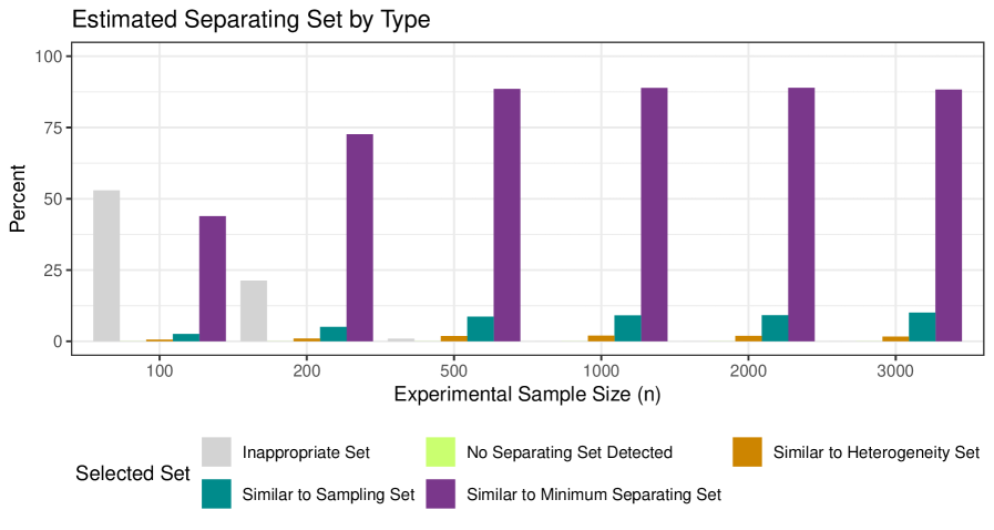
Figure SM-8: Types of Estimated Separating Sets. Note: We present the frequency of estimated separating sets by conceptual type. While the algorithm picks an inappropriate set when the sample size is small, as $n$ increases, the most likely set is the minimal separating set.

Figure SM-8 shows the breakdown of types of estimated separating sets. We group sets that are conceptually similar, and the frequency with which each set is chosen is presented. For example, if our algorithm selects the variables in the sampling set ($X4$ and $X5$) as well as an additional variable, we group these as “similar to” the sampling set. As can be seen, in these simulations as $n$ gets large, over 75% of the time, the minimal separating set (purple) is selected. Small sample size can lead to the misestimation of the MRF, and therefore selection of inappropriate sets (gray) which do not remove bias — however, the rate at which inappropriate sets are selected drops off rapidly with sample size. In the supplementary material, we show that, when incorporating user constraints that make adjustment by the minimum separating set infeasible, the algorithm selects sets similar to the sampling and heterogeneity sets with higher frequency.

SM-5.3 Additional Simulation Results

In the previous subsection, we discussed the breakdown of the different types of estimated separating sets in the simulated data generating process. Here we show the breakdown of types of estimated separating sets when incorporating user constraints in Figure SM-9. In this case, $X1$, the alternative separating set, cannot be measured in the target population, we see that the algorithm selects the sampling and heterogeneity sets with higher frequency.

Figure SM-9: Type of Estimated Marginal Separating Set with User Constraints. Note: We present the frequency of estimated separating sets by conceptual type. With user constraints, the algorithm selects each of the other types of separating sets more frequently.

Figure SM-10 presents the bias and standard error result by selected estimated separating set type. We refer to sets that are “similar to” different conceptual sets in order to group sets that control for a specific type of separating sets, but which may include extra variables. For example, if the estimated set includes $X4$, $X5$, and $X8$, we say this is similar to a sampling set ($X4$ and $X5$). As theorems tell us, it doesn’t matter what type of separating sets the algorithm estimates in the experimental data, all of them produce unbiased estimates so long as the set is an appropriate separating set (see Figure SM-10). When an inappropriate set is chosen, which is common in the $n=100$ case but rare as $n$ increases, we see that inappropriate sets do not reduce bias. As we expect, when estimated separating sets are similar to a heterogeneity set, standard errors are the smallest.

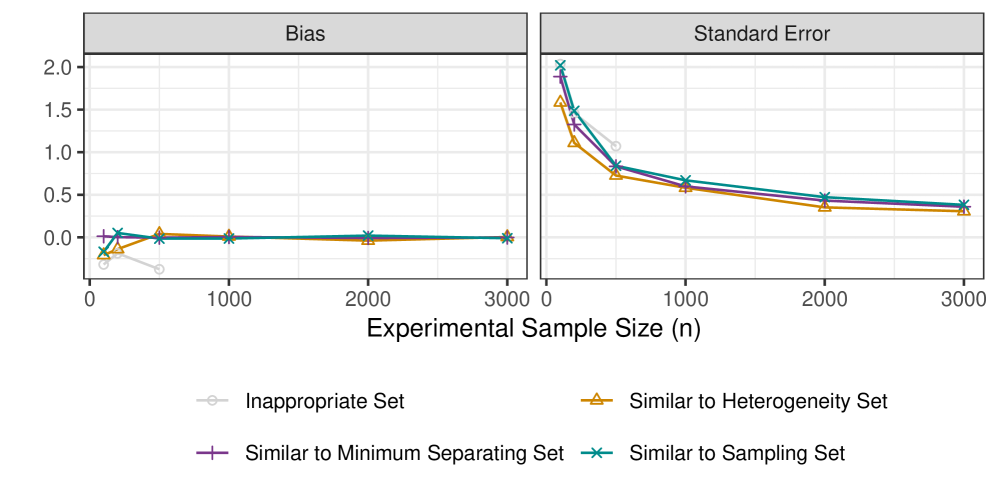
Figure SM-10: Simulation Results for Estimated Separating Set by Type. Note: The left figure shows bias for the PATE and the right figure presents standard error estimates. As expected, bias is close to zero for all estimators. Estimated sets are categorized by type: similar to oracle sampling set (green) and the oracle minimum separating set (purple) and oracle heterogeneity set (orange).

Finally, we present the simulation results for two alternative estimators in Figure SM-11, a calibration estimator and a linear regression projection. The calibration estimator matches population means for the estimated separating set using a maximum entropy (raking) algorithm [44]. The linear projection estimator estimates a fully interacted linear regression model using the estimated separating set, and projects the model on the target population.

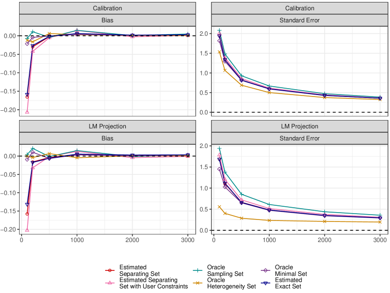
Figure SM-11: Simulation Results for Alternative Estimators. Note: The left figure shows bias for the PATE and the right figure presents standard error estimates. As expected, bias is close to zero for all estimators. More importantly, estimators based on the estimated separating sets (red) and estimated separating set with user constraints (pink) have similar standard errors to the oracle sampling set (green) and the oracle minimum separating set (purple). An estimator based on the heterogeneity set (orange) has significantly smaller standard errors than other estimators, but this estimator might be unavailable in practice.

Appendix SM-6 R Function to Estimate Separating Sets

# ################################
# Estimating the separating set
# ################################
# X.data: all pre-treatment covariates in the experimental data
# X.type: types of each covariate. "g" for continous variables, and "c" for categorical variables.
# X.level: the number of levels in each covariates. For continous variables, set it to 1.
# Y: outcome variable in the experimental data
# Treat: treatment variable in the experimental data
# XS: names of the sampling set
# XH: names of the heterogeneity set
# XU: names of variables unmeasurable in the target population
# type: when "Y", we estimate the marginal separating set. when "XH", we estimate the exact separating set.
# print_graph: whether we print the estimated Markov Random Fields

library(igraph); library(qgraph); library(lpSolve); library(mgm); library(Hmisc)

Separating <- function(X.data, X.type, X.level,
                       Y, Treat, XS, XH = NULL, XU=NULL, type = "Y",
                       print_graph = FALSE) {

  ## Setup
  n.var <- ncol(X.data)
  if(type == "Y"){
    if(missing(X.type) == TRUE){
      type.sim  <- rep("g", n.var + 2)
      level.sim <- rep(1, n.var + 2)
    }else{
      type.sim <- c(X.type, rep("g", 2))
      level.sim <- c(X.level, rep(1, 2))
    }
    X.data.g <- cbind(X.data, Y, Treat)
    name.label <- c(colnames(X.data), "Y")
  }else if(type == "XH"){
    if(missing(X.type) == TRUE){
      type.sim  <- rep("g", n.var + 1)
      level.sim <- rep(1, n.var + 1)
    }else{
      type.sim <- c(X.type, rep("g", 1))
      level.sim <- c(X.level, rep(1, 1))
    }
    X.data.g <- cbind(X.data, Treat)
    name.label <- colnames(X.data)
  }



  ## ###########################################
  ## Step 1: Estimate the Markov Random Graph
  ## ###########################################
  fit.sim <- mgm(
    data = X.data.g,
    type = type.sim,
    level = level.sim,
    threshold = "LW",
    k = 2,
    verbatim = TRUE,
    signInfo = FALSE,
    lambdaSel = "EBIC"
  )


  ## Remove T from the Graph
  treat_ind <- which(colnames(X.data.g) == "Treat")
  Ad <- as.matrix(fit.sim$pairwise$wadj > 0)
  Ad <- Ad[-treat_ind,-treat_ind]
  Ad.w <- fit.sim$pairwise$wadj
  Ad.w <- Ad.w[-treat_ind, -treat_ind]
  edge.col <- fit.sim$pairwise$edgecolor
  edge.col <- edge.col[-treat_ind,-treat_ind]
  graph.u <- graph_from_adjacency_matrix(Ad)

  ## Show the graph
  if(print_graph) qgraph(
    Ad.w,
    edge.color = edge.col,
    layout = ’spring’,
    labels = name.label
  )

  ## #################################################################
  ## Step 2: Estimate the Separating Set based on an estimated MRF
  ## #################################################################
  if (type == "Y") {
    base <- rep(0, (n.var + 1))
    XS.ind <- which(is.element(colnames(X.data), XS))
    path.cons <- matrix(NA, nrow = 0, ncol = (n.var + 1))
    ## Enumerate all path
    for (w in 1:length(XS)) {
      ind.path.mat <- do.call("rbind",
                              lapply(all_simple_paths(graph.u, (n.var + 1), XS.ind[w]),
                                     FUN=function(x) ind.path(x, base)))
      path.cons <- rbind(path.cons, ind.path.mat)
    }
  }else if (type == "XH") {
    base <- rep(0, n.var)
    XJ  <- intersect(XS, XH)
    all.pair <- expand.grid(XH, XS)
    path.cons <- matrix(NA, nrow = 0, ncol = n.var)
    ## Enumerate all path
    for (w in 1:nrow(all.pair)) {
      ind_1 <- which(colnames(X.data.g) == all.pair[w, 1])
      ind_2 <- which(colnames(X.data.g) == all.pair[w, 2])
      ind.path.mat <-
        do.call("rbind",
                lapply(
                  all_simple_paths(graph.u, ind_1, ind_2),
                  FUN=function(x) ind.path(x, base)))
      path.cons <- rbind(path.cons, ind.path.mat)
    }
  }

  if(dim(path.cons)[1] == 0) {
    solution <- NULL
    status <- 0
  }else{

    ## Removing Y and XU from the separating set
    if (length(XU) == 0) {
      if(type == "Y"){
        path.cons2 <- rbind(path.cons,
                            c(rep(0, n.var), 1))
        f.dir <- c(rep(">=", nrow(path.cons)), "=")
        f.rhs <- c(rep(1, nrow(path.cons)), 0)
      }else if(type == "XH"){
        path.cons2 <- path.cons
        f.dir <- rep(">=", nrow(path.cons))
        f.rhs <- rep(1, nrow(path.cons))
      }
    } else{
      XU.ind <- which(is.element(colnames(X.data), XU))
      path.cons2.u <- matrix(0, nrow = length(XU.ind), ncol = n.var)
      for (i in 1:nrow(path.cons2.u)) {
        path.cons2.u[i, XU.ind[i]] <- 1
      }
      if(type == "Y"){
        path.cons2.u2 <- cbind(path.cons2.u, 0)
        path.cons2 <- rbind(path.cons,
                            c(rep(0, n.var), 1),
                            path.cons2.u2)
        f.dir <- c(rep(">=", nrow(path.cons)),
                   rep("=", (nrow(path.cons2.u2) + 1)))
        f.rhs <- c(rep(1, nrow(path.cons)),
                   rep(0, (nrow(path.cons2.u2) + 1)))
      }else if(type == "XH"){
        path.cons2.u2 <- path.cons2.u
        path.cons2 <- rbind(path.cons,
                            path.cons2.u2)
        f.dir <- c(rep(">=", nrow(path.cons)),
                   rep("=", nrow(path.cons2.u2)))
        f.rhs <- c(rep(1, nrow(path.cons)),
                   rep(0, nrow(path.cons2.u2)))
      }
    }

    if(type == "Y"){f.obj <- c(rep(1, n.var), 0)}
    else if(type == "XH"){f.obj <- rep(1, n.var)}
    f.con <- path.cons2

    num.solutions <- max.solutions.calculate <- 1
    sp.out <- lp("min", f.obj, f.con, f.dir, f.rhs, all.bin = TRUE, num.bin.solns = max.solutions.calculate)
    if(sp.out$status == 0) {
      if(max.solutions.calculate > 1) {
        solution <- sp.out$solution[1:(length(f.obj)*max.solutions.calculate)]
        solution <- split(solution, sort(1:length(solution) %% sp.out$num.bin.solns))
        if(num.solutions == 1) {
          solution <- sample(solution, num.solutions)
        }
        if(length(solution) == 1) {
          solution <- as.vector(unlist(solution))
        }
      } else {
        solution <- sp.out$solution
      }
    }
    status <- sp.out$status
  }

  ## Final Adjustment
  if (status == 0) {
    if(is.null(solution)==TRUE) {
      ## the empty set is enough for generalizability
      solution.name <- NULL
    }else{
      if(type == "Y"){
        solution.ind <-  which(solution[-length(solution)] == 1)
        XJ <- NULL
      }else if (type == "XH") {
        solution.ind <-  which(solution == 1)
      }
      solution.name <- colnames(X.data)[solution.ind]
      if(type == "XH" & length(XJ)!=0){ solution.name <- union(solution.name, XJ)}
    }
  }else if (status==2){
    cat("\nNo Feasible Solution.\n")
    solution.name <- "No Feasible Solution."
  }

  if(print_graph==TRUE){cat ("\n"); cat(solution.name)}

  return(solution.name)
}

# Auxiliary function
ind.path <- function(x, base) {
  base[x] <- 1
  return(base)
}

References

- [1] Hunt Allcott “Site selection bias in program evaluation” In Quarterly Journal of Economics, 2015, pp. 1117–1165
- [2] Isaiah Andrews and Emily Oster “A Simple Approximation For Evaluating External Validity Bias” In Economics Letters 178 Elsevier, 2019, pp. 58–62
- [3] Joshua D Angrist and Jörn-Steffen Pischke “The Credibility Revolution in Empirical Economics: How Better Research Design Is Taking the Con out of Econometrics” In Journal of Economic Perspectives 24.2, 2010, pp. 3–30
- [4] Elias Bareinboim and Judea Pearl “Causal Inference and the Data-Fusion Problem” In Proceedings of the National Academy of Sciences 113.27 National Academy of Sciences, 2016, pp. 7345–7352
- [5] Elias Bareinboim, Jin Tian and Judea Pearl “Recovering from Selection Bias in Causal and Statistical Inference” In Twenty-Eighth AAAI Conference on Artificial Intelligence, 2014
- [6] Christopher Blattman, Nathan Fiala and Sebastian Martinez “Generating Skilled Self-Employment in Developing Countries: Experimental Evidence from Uganda” In The Quarterly Journal of Economics 129.2 MIT Press, 2013, pp. 697–752
- [7] Ashley L Buchanan et al. “Generalizing evidence from randomized trials using inverse probability of sampling weights” In Journal of the Royal Statistical Society. Series A (Statistics in Society) 95, 2018, pp. 1082
- [8] Wendy Chan “Partially Identified Treatment Effects for Generalizability” In Journal of Research on Educational Effectiveness 10.3, 2017, pp. 646–669
- [9] Stephen R Cole and Elizabeth A Stuart “Generalizing Evidence From Randomized Clinical Trials to Target PopulationsThe ACTG 320 Trial” In American journal of epidemiology 172.1, 2010, pp. 107–115
- [10] Bénédicte Colnet et al. “Causal inference methods for combining randomized trials and observational studies: a review” In arXiv preprint arXiv:2011.08047, 2020
- [11] Issa J Dahabreh et al. “Extending Inferences From A Randomized Trial To A New Target Population” In Statistics in Medicine 39.14 Wiley Online Library, 2020, pp. 1999–2014
- [12] Issa J Dahabreh et al. “Generalizing Causal Inferences From Individuals In Randomized Trials to All Trial-Eligible Individuals” In Biometrics 75.2 Wiley Online Library, 2019, pp. 685–694
- [13] Angus Deaton and Nancy Cartwright “Understanding and Misunderstanding Randomized Controlled TYrials” In Social Science & Medicine, 2018
- [14] James N Druckman, Donald P Green, James H Kuklinski and Arthur Lupia “Cambridge Handbook of Experimental Political Science” Cambridge University Press, 2011
- [15] Esther Duflo and Michael Kremer “Use of Randomization in the Evaluation of Development Effectiveness” In Evaluating Development Effectiveness New Brunswick, NJ: Transaction Publishers, 2005, pp. 205–232
- [16] Government of Uganda “National Peace, Recovery and Development Plan for Northern Uganda: 2006–2009”, 2007
- [17] Erin Hartman, Richard Grieve, Roland Ramsahai and Jasjeet S Sekhon “From sample average treatment effect to population average treatment effect on the treated: combining experimental with observational studies to estimate population treatment effects” In Journal of the Royal Statistical Society. Series A (Statistics in Society) 178.3, 2015, pp. 757–778
- [18] Jonas Haslbeck and Lourens J Waldorp “mgm: Estimating Time-Varying Mixed Graphical Models in High-Dimensional Data” In Journal of Statistical Software 93.8, 2020, pp. 1–46
- [19] Kosuke Imai, Gary King and Elizabeth A Stuart “Misunderstandings between experimentalists and observationalists about causal inference” In Journal of the Royal Statistical Society: Series A (Statistics in Society) 171.2 Blackwell Publishing Ltd, 2008, pp. 481–502
- [20] Guido W Imbens “Better LATE Than Nothing: Some Comments on Deaton (2009) and Heckman and Urzua (2009)” In Journal of Economic Literature 48.2, 2010, pp. 399–423
- [21] Guido W Imbens and Donald B Rubin “Causal Inference in Statistics, Social, and Biomedical Sciences” Cambridge University Press, 2015
- [22] Holger L Kern, Elizabeth A Stuart, Jennifer Hill and Donald P Green “Assessing Methods for Generalizing Experimental Impact Estimates to Target Populations” In Journal of Research on Educational Effectiveness 9.1, 2016, pp. 103–127
- [23] Steffen L Lauritzen “Graphical Models” Oxford: Clarendon Press, 1996
- [24] Nicolai Meinshausen and Peter Bühlmann “High-Dimensional Graphs and Variable Selection with the Lasso” In The Annals of Statistics 34.3, 2006, pp. 1436–1462
- [25] Luke W. Miratrix, Jasjeet S. Sekhon, Alexander G. Theodoridis and Luis F. Campos “Worth Weighting? How to Think About and Use Weights in Survey Experiments” In Political Analysis 26.3 Cambridge University Press, 2018, pp. 275–291 DOI: 10.1017/pan.2018.1
- [26] Rachel C Nethery, Fabrizia Mealli and Francesca Dominici “Estimating Population Average Causal Effects in the Presence of Non-Overlap: The Effect of Natural Gas Compressor Station Exposure on Cancer Mortality” In The Annals of Applied Statistics 13.2 NIH Public Access, 2019, pp. 1242
- [27] Jerzy Neyman “On the Application of Probability Theory to Agricultural Experiments. Essay on Principles (with discussion). Section 9 (translated)” In Statistical Science 5.4 Institute of Mathematical Statistics, 1923, pp. 465–472
- [28] Trang Quynh Nguyen et al. “Sensitivity Analyses for Effect Modifiers Not Observed in The Target Population When Generalizing Treatment Effects From A Randomized Controlled Trial: Assumptions, Models, Fffect scales, Data scenarios, and Implementation Details” In PloS one 13.12 Public Library of Science San Francisco, CA USA, 2018, pp. e0208795
- [29] Trang Quynh Nguyen, Cyrus Ebnesajjad, Stephen R Cole and Elizabeth A Stuart “Sensitivity analysis for an unobserved moderator in RCT-to-target-population generalization of treatment effects” In The Annals of Applied Statistics 11.1, 2017, pp. 225–247
- [30] Judea Pearl and Elias Bareinboim “External Validity: From Do-Calculus to Transportability Across Populations” In Statistical Science 29.4, 2014, pp. 579–595
- [31] Taylor R Pressler and Eloise E Kaizar “The use of propensity scores and observational data to estimate randomized controlled trial generalizability bias” In Statistics in medicine 32.20 Wiley Online Library, 2013, pp. 3552–3568
- [32] Donald B Rubin “Estimating causal effects of treatments in randomized and nonrandomized studies.” In Journal of educational Psychology 66.5 American Psychological Association, 1974, pp. 688
- [33] Donald B Rubin “Comment on J. Neyman and causal inference in experiments and observational studies: “On the application of probability theory to agricultural experiments. Essay on principles. Section 9” [Ann. Agric. Sci. 10 (1923), 1–51]” In Statistical Science 5.4, 1990, pp. 472–480
- [34] Alastair J Scott and CJ Wild “Fitting Logistic Models Under Case-Control Or Choice Based Sampling” In Journal of the Royal Statistical Society: Series B (Methodological) 48.2 Wiley Online Library, 1986, pp. 170–182
- [35] William R Shadish, Thomas D Cook and Donald T Campbell “Experimental and Quasi-Experimental Designs for Generalized Causal Inference” Boston: Houghton Mifflin, 2002
- [36] Elizabeth A Stuart, Catherine P Bradshaw and Philip J Leaf “Assessing the Generalizability of Randomized Trial Results to Target Populations” In Prevention Science 16.3, 2015, pp. 475–485
- [37] Elizabeth A Stuart, Stephen R Cole, Catherine P Bradshaw and Philip J Leaf “The Use of Propensity Scores to Assess the Generalizability of Results from Randomized Trials” In Journal of the Royal Statistical Society. Series A (Statistics in Society) 174.2, 2011, pp. 369–386
- [38] Elizabeth Tipton “Improving Generalizations From Experiments Using Propensity Score Subclassification: Assumptions, Properties, and Contexts” In Journal of Educational and Behavioral Statistics 38.3, 2013, pp. 239–266
- [39] Elizabeth Tipton et al. “Site Selection in Experiments: An Assessment of Site Recruitment and Generalizability in Two Scale-Up Studies” In Journal of Research on Educational Effectiveness 9.sup1 Taylor & Francis, 2016, pp. 209–228
- [40] Daniel Westreich et al. “Transportability of Trial Results Using Inverse Odds of Sampling Weights” In American Journal of Epidemiology 186.8 Oxford University Press, 2017, pp. 1010–1014
- [41] World Bank “World Development Report 2013: Jobs”, 2012
- [42] Eunho Yang, Pradeep Ravikumar, Genevera I Allen and Zhandong Liu “Graphical Models via Univariate Exponential Family Distributions” In Journal of Machine Learning Research 16.1, 2015, pp. 3813–3847
- [43] Issa J Dahabreh et al. “Generalizing Causal Inferences From Individuals In Randomized Trials to All Trial-Eligible Individuals” In Biometrics 75.2 Wiley Online Library, 2019, pp. 685–694
- [44] Erin Hartman, Richard Grieve, Roland Ramsahai and Jasjeet S Sekhon “From sample average treatment effect to population average treatment effect on the treated: combining experimental with observational studies to estimate population treatment effects” In Journal of the Royal Statistical Society. Series A (Statistics in Society) 178.3, 2015, pp. 757–778
- [45] Steffen L Lauritzen “Graphical Models” Oxford: Clarendon Press, 1996
- [46] Judea Pearl “Causality: Models, Reasoning and Inference” Cambridge University Press, 2000
- [47] James M Robins, Andrea Rotnitzky and Lue Ping Zhao “Estimation of Regression Coefficients When Some Regressors Are Not Always Observed” In Journal of the American Statistical Association 89.427 Taylor & Francis, 1994, pp. 846–866
Supplementary Material