Additive function approximation in the brain

Abstract

Many biological learning systems such as the mushroom body, hippocampus, and cerebellum are built from sparsely connected networks of neurons. For a new understanding of such networks, we study the function spaces induced by sparse random features and characterize what functions may and may not be learned. A network with $d$ inputs per neuron is found to be equivalent to an additive model of order $d$, whereas with a degree distribution the network combines additive terms of different orders. We identify three specific advantages of sparsity: additive function approximation is a powerful inductive bias that limits the curse of dimensionality, sparse networks are stable to outlier noise in the inputs, and sparse random features are scalable. Thus, even simple brain architectures can be powerful function approximators. Finally, we hope that this work helps popularize kernel theories of networks among computational neuroscientists.

1 Introduction

Kernel function spaces are popular among machine learning researchers as a potentially tractable framework for understanding artificial neural networks trained via gradient descent [e.g. bach2017, jacot2018, chizat2018, mei2018, rotskoff2018, venturi2018]. Artificial neural networks are an area of intense interest due to their often surprising empirical performance on a number of challenging problems and our still incomplete theoretical understanding. Yet computational neuroscientists have not widely applied these new theoretical tools to describe the ability of biological networks to perform function approximation.

The idea of using fixed random weights in a neural network is primordial, and was a part of Rosenblatt’s perceptron model of the retina [rosenblatt1958]. Random features have then resurfaced under many guises: random centers in radial basis function networks [broomhead1988], functional link networks [igelnik1995], Gaussian processes (GPs) [neal1996, williams1997], and so-called extreme learning machines [wang2008]; see [scardapane2017] for a review. Random feature networks, where the neurons are initialized with random weights and only the readout layer is trained, were proposed by Rahimi and Recht in order to improve the performance of kernel methods [rahimi2008, rahimi2008a] and can perform well for many problems [scardapane2017].

In parallel to these developments in machine learning, computational neuroscientists have also studied the properties of random networks with a goal towards understanding neurons in real brains. To a first approximation, many neuronal circuits seem to be randomly organized [ganguli2012, caron2013, caron2013a, harris2017, litwin-kumar2017]. However, the recent theory of random features appears to be mostly unknown to the greater computational neuroscience community.

Here, we study random feature networks with sparse connectivity: the hidden neurons each receive input from a random, sparse subset of input neurons. This is inspired by the observation that the connectivity in a variety of predominantly feedforward brain networks is approximately random and sparse. These brain areas include the cerebellar cortex, invertebrate mushroom body, and dentate gyrus of the hippocampus [cayco-gajic2019]. All of these areas perform pattern separation and associative learning. The cerebellum is important for motor control, while the mushroom body and dentate gyrus are general learning and memory areas for invertebrates and vertebrates, respectively, and may have evolved from a similar structure in the ancient bilaterian ancestor [wolff2016]. Recent work has argued that the sparsity observed in these areas may be optimized to balance the dimensionality of representation with wiring cost [litwin-kumar2017]. Sparse connectivity has been used to compress neural networks and speed up computation [han2015, han2015a, wen2016], whereas convolutions are a kind of structured sparsity [mairal2014, jones2019].

We show that sparse random features approximate additive kernels [wahba1990, bach2009, duvenaud2011, kandasamy2016] with arbitrary orders of interaction. The in-degree of the hidden neurons $d$ sets the order of interaction. When the degrees of the neurons are drawn from a distribution, the resulting kernel contains a weighted mixture of interactions. These sparse features offer advantages of generalization in high-dimensions, stability under perturbations of their input, and computational and biological efficiency.

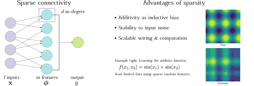
Figure 1: Sparse connectivity in a shallow neural network. The function shown is the sparse random feature approximation to an additive sum of sines, learned from poorly distributed samples (red crosses). Additivity offers structure which may be leveraged for fast and efficient learning.

2 Background: Random features and kernels

Now we will introduce the mathematical setting and review how random features give rise to kernels. The simplest artificial neural network contains a single hidden layer, of size $m$, receiving input from a layer of size $l$ (Figure 1). The activity in the hidden layer is given by, for $i\in[m]$,

$$\phi_{i}(\mathbf{x})=h(\mathbf{w}^{\intercal}_{i}\mathbf{x}+b_{i}).$$ (1)

Here each $\phi_{i}$ is a feature in the hidden layer, $h$ is the nonlinearity, $\mathbf{W}=(\mathbf{w}_{1},\mathbf{w}_{2},\ldots,\mathbf{w}_{m})\in\mathbb{R}^{l\times m}$ are the input to mixed weights, and $\mathbf{b}\in\mathbb{R}^{m}$ are their biases. We can write this in vector notation as $\bm{\phi}(\mathbf{x})=h(\mathbf{W}^{\intercal}\mathbf{x}-\mathbf{b})$, where $\bm{\phi}:\mathbb{R}^{l}\to\mathbb{R}^{m}$.

Random features networks are draw their input-hidden layer weights at random. Let the weights $\mathbf{W}$ and biases $\mathbf{b}$ in the feature expansion (1) be sampled i.i.d. from a distribution $\mu$ on $\mathbb{R}^{l+1}$. Under mild assumptions, the inner product of the feature vectors for two inputs converges to its expectation

$$\frac{1}{m}\bm{\phi}(\mathbf{x})^{\intercal}\bm{\phi}(\mathbf{x}^{\prime})\xrightarrow{m\to\infty}\mathbb{E}\left[\phi(\mathbf{x})\phi(\mathbf{x}^{\prime})\right]=\int h(\mathbf{w}^{\intercal}\mathbf{x}+b)h(\mathbf{w}^{\intercal}\mathbf{x}^{\prime}+b)\,\mathrm{d}\mu(\mathbf{w},b):=k(\mathbf{x},\mathbf{x}^{\prime}).$$ (2)

We identify the limit (2) with a reproducing kernel $k(\mathbf{x},\mathbf{x}^{\prime})$ induced by the random features, since the limiting function is an inner product and thus always positive semidefinite [rahimi2008]. The kernel defines an associated reproducing kernel Hilbert space (RKHS) of functions. For a finite network of width $m$, the inner product $\frac{1}{m}\bm{\phi}(\mathbf{x})^{\intercal}\bm{\phi}(\mathbf{x}^{\prime})$ is a randomized approximation to the kernel $k(\mathbf{x},\mathbf{x}^{\prime})$.

3 Sparsely connected random feature kernels

We now turn to our main result: the general form of the random feature kernels with sparse, independent weights. For simplicity, we start with a regular model and then generalize the result to networks with varying in-degree. Two kernels that can be computed in closed form are highlighted.

Fix an in-degree $d$, where $1\leq d\leq l$, and let $\mu|d$ be a distribution on $\mathbb{R}^{d}$ which induce, together with some nonlinearity $h$, the kernel $k_{d}(\mathbf{z},\mathbf{z}^{\prime})$ on $\mathbf{z},\mathbf{z}^{\prime}\in\mathbb{R}^{d}$ (for the moment, $d$ is not random). Sample a sparse feature $i\in[m]$ in two steps: First, pick $d$ neighbors from all $\binom{l}{d}$ uniformly at random. Let $\mathcal{N}_{i}\subseteq[l]$ denote this set of neighbors. Second, sample $w_{ji}\sim\mu|d$ if $j\in\mathcal{N}_{i}$ and otherwise set $w_{ji}=0$. We find that the resulting kernel

$$k_{d}^{\mathrm{reg}}(\mathbf{x},\mathbf{x}^{\prime})=\mathbb{E}[\mathbb{E}[\phi(\mathbf{x}_{\mathcal{N}})\phi(\mathbf{x}^{\prime}_{\mathcal{N}})|\mathcal{N}]]={\binom{l}{d}^{-1}}\sum_{\mathcal{N}:|\mathcal{N}|=d}k_{d}(\mathbf{x}_{\mathcal{N}},\mathbf{x}^{\prime}_{\mathcal{N}}).$$ (3)

Here $\mathbf{x}_{\mathcal{N}}$ denotes the length $d$ vector of $\mathbf{x}$ restricted to the neighborhood $\mathcal{N}$, with the other $l-d$ entries in $\mathbf{x}$ ignored.

More generally, the in-degrees may be chosen independently according to a degree distribution, so that $d$ becomes a random variable. Let $D(d)$ be the probability mass function of the hidden node in-degrees. Conditional on node $i$ having degree $d_{i}$, the in-neighborhood $\mathcal{N}_{i}$ is chosen uniformly at random among the $\binom{l}{d_{i}}$ possible sets. Then the induced kernel becomes

$$k_{D}^{\mathrm{dist}}(\mathbf{x},\mathbf{x}^{\prime})=\mathbb{E}[\mathbb{E}[\phi(\mathbf{x}_{\mathcal{N}})\phi(\mathbf{x}^{\prime}_{\mathcal{N}})|\mathcal{N},d]]=\sum_{d=0}^{l}D(d)\,k_{d}^{\mathrm{reg}}(\mathbf{x},\mathbf{x}^{\prime}).$$ (4)

For example, if every layer-two node chooses its inputs independently with probability $p$, the $D(d_{i})$ is the probability mass function of the binomial distribution $\mathrm{Bin}(l,p)$. The regular model (3) is a special case of (4) with $D(d^{\prime})=\mathbb{I}{\{d^{\prime}=d\}}$. Extending the proof techniques in [rahimi2008] yields:

Claim The random map $\frac{1}{m}\bm{\phi}(\mathbf{x})^{\intercal}\bm{\phi}(\mathbf{x}^{\prime})$ with $\kappa$-Lipschitz nonlinearity uniformly approximates $k_{D}^{\mathrm{dist}}(\mathbf{x},\mathbf{x}^{\prime})$ to error $\epsilon$ using $m=\Omega(\frac{l\kappa^{2}}{\epsilon^{2}}\log\frac{C}{\epsilon})$ many features (the proof is contained in Appendix C).

Two simple examples

With Gaussian weights and regular $d=1$, we find that (see Appendix B)

$$k_{1}^{\mathrm{reg}}(\mathbf{x},\mathbf{x}^{\prime}) =1-\frac{1}{l}\|\mathrm{sgn}(\mathbf{x})-\mathrm{sgn}(\mathbf{x}^{\prime})\|_{0} h=$$ if step function, and (5)

$$k_{1}^{\mathrm{reg}}(\mathbf{x},\mathbf{x}^{\prime}) =1-\frac{c}{l}\|\mathbf{x}-\mathbf{x}^{\prime}\|_{1} \mbox{if $h=$ sign function}.$$ (6)

4 Advantages of sparse connectivity

4.1 Additive modeling

The regular degree kernel (3) is a sum of kernels that only depend on combinations of $d$ inputs, making it an additive kernel of order $d$. The general expression for the degree distribution kernel (4) illustrates that sparsity leads to a mixture of additive kernels of different orders. These have been referred to as additive GPs [duvenaud2011], but these kind of models have a long history as generalized additive models [e.g. wahba1990, hastie2009]. For the regular degree model with $d=1$, the sum in (3) is over neighborhoods of size one, simply the individual indices of the input space. Thus, for any two input neighborhoods $\mathcal{N}_{1}$ and $\mathcal{N}_{2}$, we have $|\mathcal{N}_{1}\cap\mathcal{N}_{2}|=\emptyset$, and the RKHS corresponding to $k_{1}^{\mathrm{reg}}(\mathbf{x},\mathbf{x}^{\prime})$ is the direct sum of the subspaces $\mathcal{H}=\mathcal{H}_{1}\oplus\ldots\oplus\mathcal{H}_{l}$. Thus regular $d=1$ defines a first-order additive model, where $f(\mathbf{x})=f_{1}(x_{1})+\ldots+f_{l}(x_{l})$. When $d>1$ we allow interactions between subsets of $d$ variables, e.g. regular $d=2$ leads to $f(\mathbf{x})=f_{12}(x_{1},x_{2})+\ldots+f_{l-1,l}(x_{l-1},x_{l})$, all pairwise terms. These interactions are defined by the structure of the terms $k_{d}(\mathbf{x}_{\mathcal{N}},\mathbf{x}^{\prime}_{\mathcal{N}})$. Finally, the degree distribution $D(d)$ determines how much weight to place on different degrees of interaction.

Generalization from fewer examples in high dimensions

Stone proved that first-order additive models do not suffer from the curse of dimensionality [stone1985, stone1986], as the excess risk does not depend on the dimension $l$. kandasamy2016 extended this result to $d$th-order additive models and found a bound on the excess risk of $O(l^{2d}n^{\frac{-2s}{2s+d}})$ or $O(l^{2d}C^{d}/n)$ for kernels with polynomial or exponential eigenvalue decay rates ($n$ is the number of samples and the constants $s$ and $C$ parametrize rates). Without additivity, these weaken to $O(n^{\frac{-2s}{2s+l}})$ and $O(C^{l}/n)$, much worse when $l\gg d$.

Similarity to dropout

Dropout regularization [hinton2012, srivastava2013] in deep networks has been analyzed in a kernel/GP framework [duvenaud2014], leading to (4) with $D=\mathrm{Bin}(l,p)$ for a particular base kernel. Dropout may thus improve generalization by enforcing approximate additivity, for the reasons above.

4.2 Stability: robustness to noise or attacks affecting a few inputs

Equations (5) and (6) are similar: They differ only by the presence of an $\ell^{0}$-“norm” versus an $\ell^{1}$-norm and the presence of the sign function. Both norms are stable to outlying coordinates in an input $\mathbf{x}$. This property also holds for $1<d\ll l$, since every feature $\phi_{i}(\mathbf{x})$ only depends on $d$ inputs, and therefore only a minority of the $m$ features will be affected by the few outliers. Thus, sufficiently sparse features will be less affected by sparse noise than a fully-connected network. Furthermore, any regressor $f(\mathbf{x})=\bm{\alpha}^{\intercal}\bm{\phi}(\mathbf{x})$ built from these features will also be stable. By Cauchy-Schwartz, $|f(\mathbf{x})-f(\mathbf{x}^{\prime})|\leq\|\bm{\alpha}\|_{2}\|\bm{\phi}(\mathbf{x})-\bm{\phi}(\mathbf{x}^{\prime})\|_{2}$. Thus if $\mathbf{x}^{\prime}=\mathbf{x}+\mathbf{e}$ where $\mathbf{e}$ is noise with small number of nonzero entries, then $f(\mathbf{x}^{\prime})\approx f(\mathbf{x})$ since $\bm{\phi}(\mathbf{x})\approx\bm{\phi}(\mathbf{x}^{\prime})$. The network intrinsically denoises its inputs, which may offer advantages [e.g. litwin-kumar2017]. Stability also may guarantee the robustness of networks to adversarial attacks [lecuyer2018, cohen2019, salman2019], thus sparse networks are robust to attacks on only a few inputs.

4.3 Scalability: computational and biological

Computational

Sparse random features give potentially huge improvements in scaling. Direct implementations of additive models incur a large cost for $d>1$, since (3) requires a sum over $\binom{l}{d}=O(l^{d})$ neighborhoods. This leads to $O(n^{2}l^{d})$ time to compute the Gram matrix of $n$ examples and $O(nl^{d})$ operations to evaluate $f(\mathbf{x})$. In our case, since the random features method is primal, we need to perform $O(nmd)$ computations to evaluate the feature matrix and the cost of evaluating $f(\mathbf{x})$ remains $O(md)$. Sparse matrix-vector multiplication makes evaluation faster than the $O(ml)$ time it takes when connectivity is dense. For ridge regression, we have the usual advantages that computing an estimator takes $O(nm^{2}+nmd)$ time and $O(nm+md)$ memory, rather than $O(n^{3})$ time and $O(n^{2})$ memory for a naïve kernel ridge method.

Biological

In a small animal such as a flying insect, space is extremely limited. Sparsity offers a huge advantage in terms of wiring cost [litwin-kumar2017]. Additive approximation also means that such animals can learn much more quickly, as seen in the mushroom body [huerta2009, delahunt2019, delahunt2018a]. While the previous computational points do not apply as well to biology, since real neurons operate in parallel, fewer operations translate into lower metabolic cost for the animal.

5 Discussion

Inspired by their ubiquity in biology, we have studied sparse random networks of neurons using the theory of random features, finding the advantages of additivity, stability, and scalability. This theory shows that sparse networks such as those found in the mushroom body, cerebellum, and hippocampus can be powerful function approximators. Kernel theories of neural circuits may be more broadly applicable in the field of computational neuroscience.

Expanding the theory of dimensionality in neuroscience

Learning is easier in additive function spaces because they are low-dimensional, a possible explanation for few-shot learning in biological systems. Our theory is complementary to existing theories of dimensionality in neural systems [ganguli2012, rigotti2013, babadi2014, meister2015, mazzucato2016, litwin-kumar2017, gao2017, mastrogiuseppe2018, farrell2019], which defined dimensionality using a (debatably) ad hoc skewness measure of covariance eigenvalues. Kernel theory extends this concept, measuring dimensionality similarly [zhang2005] in the space of nonlinear functions spanned by the kernel.

Limitations

We model biological neurons as simple scalar functions, completely ignoring time and neuromodulatory context. It seems possible that a kernel theory could be developed for time- and context-dependent features. Our networks suppose i.i.d. weights, but weights that follow Dale’s law should also be considered. We have not studied the sparsity of activity, postulated to be relevant in cerebellum. It remains to be demonstrated how the theory can make concrete, testable predictions, e.g. whether this theory may explain identity versus concentration encoding of odors or the discrimination/generalization tradeoff under experimental conditions.

Acknowledgments

KDH was supported by a Washington Research Foundation postdoctoral fellowship. Thank you to Rajesh Rao for support during this project and to Bing Brunton for support and many helpful comments.

Appendices: Additive function approximation in the brain

Table of contents

• Appendix A: Test problems and numerical experiments

• Appendix B: Kernel examples arising from random features, dense and sparse

• Appendix C: Kernel approximation results, uniform convergence of Lipschitz features

Appendix A Test problems

We have implemented sparse random features in Python to demonstrate the properties of learning in this basis. Our code, which provides a scikit-learn style SparseRFRegressor and SparseRFClassifier estimators, is available from https://github.com/kharris/sparse-random-features.

A.1 Additive function approximation

A.1.1 Comparison with datasets from kandasamy2016

As said in the main text, kandasamy2016 created a theory of the generalization properties of higher-order additive models. They supplemented this with an empirical study of a number of datasets using their Shrunk Additive Least Squares Approximation (SALSA) implementation of the additive kernel ridge regression (KRR). Their data and code were obtained from https://github.com/kirthevasank/salsa.

We compared the performance of SALSA to the sparse random feature approximation of the same kernel. We employ random sparse Fourier features with Gaussian weights $N(0,\sigma^{2}\mathbf{I})$ with $\sigma=0.05\cdot\sqrt{d}n^{1/5}$ in order to match the Gaussian radial basis function used by kandasamy2016. We use $m=300l$ features for every problem, with regular degree $d$ selected equal to the one chosen by SALSA. The regressor on the features is cross-validated ridge regression (RidgeCV from scikit-learn) with ridge penalty selected from 5 logarithmically spaced points between $10^{-4}\cdot n$ and $10^{2}\cdot n$.

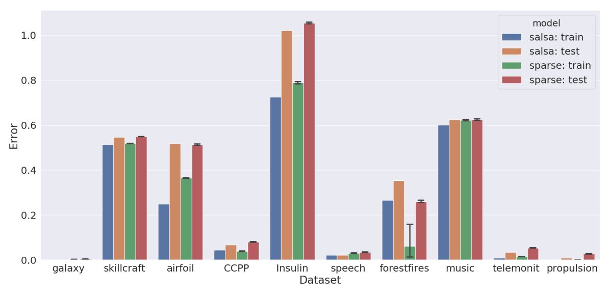
Figure 2: Comparison of sparse random feature approximation to additive kernel method SALSA [kandasamy2016]. The parameters were matched between the two models (see text). The sparse feature approximation performs slightly worse than the exact method, but similar.

In Figure 2, we compare the performance of sparse random features to SALSA. Generally, the training and testing errors of the sparse model are slightly higher than for the kernel method, except for the forestfires dataset.

A.1.2 Polynomial test function shows generalization from fewer examples

We studied the speed of learning for a test function as well. The function to be learned $f(\mathbf{x})$ was a sparse polynomial plus a linear term:

$$f(\mathbf{x})=c_{1}\mathbf{a}^{\intercal}\mathbf{x}+c_{2}\,p(\mathbf{x}).$$

The linear term took $\mathbf{a}\sim N(0,\mathbf{I})$, the polynomial $p$ was chosen to have 3 terms of degree 3 with weights drawn from $N(0,1)$. The inputs $\mathbf{x}$ are drawn from the uniform distribution over $[0,1]^{16}$. Gaussian noise $\epsilon$ with variance $0.05^{2}$ was added to generate observations $y_{i}=f(\mathbf{x}_{i})+\epsilon_{i}$. Constants $c_{1}$ and $c_{2}$ were tuned by setting $c_{1}=\frac{1}{\sigma_{\mathrm{lin}}}\frac{1-\alpha}{\sqrt{\alpha^{2}+(1-\alpha)^{2}}}$ and $c_{2}=\frac{1}{\sigma_{\mathrm{nonlin}}}\frac{\alpha}{\sqrt{\alpha^{2}+(1-\alpha)^{2}}}$, where $\alpha=0.05$ and $\sigma_{\mathrm{lin}}$ and $\sigma_{\mathrm{nonlin}}$ were the standard deviations of the linear and nonlinear terms alone.

For this problem we use random features of varying regular degrees $d=1,3,10,16$ and number of data points $n$. The features use a Fourier nonlinearity $h(\cdot)=(\sin\cdot,\cos\cdot)$, weights $w_{ij}\sim N(0,d^{-1/2})$, and biases $b_{i}\sim U([-\pi,\pi])$, leading to an RBF kernel in $d$ dimensions. The output regression model is again ridge regression with the penalty selected via cross-validation on the training set from 7 logarithmically spaced points between $10^{-4}$ and $10^{2}$.

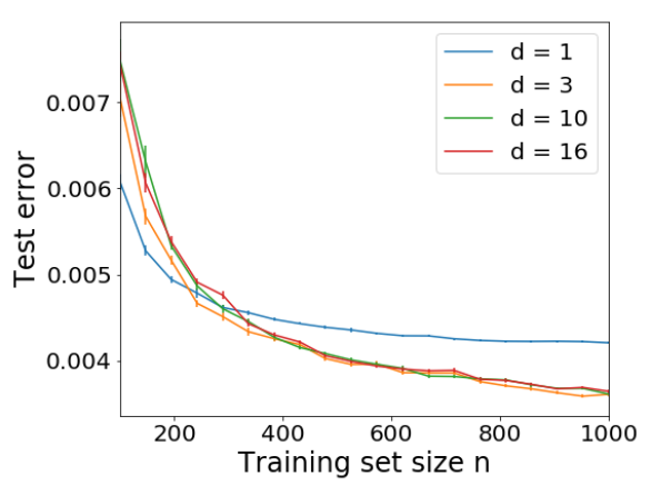
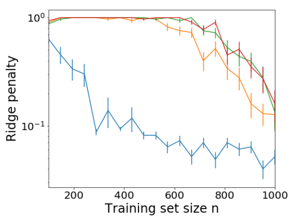
Figure 3: Performance of sparse random features of differing degree $d$ and training size $n$ for the polynomial test function. Test error is measured as mean square error with noise floor at 0.0025. As the amount of training data increases, higher $d$, i.e. more model complexity, is preferred.

In Figure 3, we show the test error as well as the selected ridge penalty for different values of $d$ and $n$. With a small amount of data ($n<250$), the model with $d=1$ has the lowest test error, since this “simplest” model is less likely to overfit. On the other hand, in the intermediate data regime ($250<n<400$), the model with $d=3$ does best. For large amounts of data ($n>400$), all of the models with interactions $d\geq 3$ do roughly the same. Note that with the RBF kernel the RKHS $\mathcal{H}_{d}\subseteq\mathcal{H}_{d^{\prime}}$ whenever $d\leq d^{\prime}$, so $d>3$ can still capture the degree 3 polynomial model. However, we see that the more complex models have a higher ridge penalty selected. The penalty is able to adaptively control this complexity given enough data.

A.2 Stability with respect to sparse input noise

Here we show that sparse random features are stable for spike-and-slab input noise. In this example, the truth follows a linear model, where we have random input points $\mathbf{x}_{i}\sim\mathcal{N}(0,\mathbf{I})$ and linear observations $y_{i}=\mathbf{x}_{i}^{\intercal}\beta$ for $i=1,\ldots,n$ and $\beta\sim\mathcal{N}(0,\mathbf{I})$. However, we only have access to sparsely corruputed inputs $\mathbf{w}_{i}=\mathbf{x}_{i}+\mathbf{e}_{i}$, where $\mathbf{e}_{i}=0$ with probability $1-p$ and $\mathbf{e}_{i}=\bm{\epsilon}_{x}-\mathbf{x}_{i}$ with probability $p$, $\bm{\epsilon}_{x}\sim\mathcal{N}(0,\sigma^{2}\mathbf{I})$. That is, the corrupted inputs are replaced with pure noise. We use $p=0.03\ll 1$ and $\sigma=6\gg 1$ so that the noise is sparse but large when it occurs.

Model	Training score	Testing score
Linear	0.854	0.453
Kernel	1.000	0.607
Trim + linear	0.945	0.686
Huber	0.858	0.392

Table 1: Scores ($R^{2}$ coefficient) of various regression models on linear data with corrupted inputs. In the presence of these errors, linear regression fails to acheive as good a test score as the kernel method, which is almost as good as trimming before performing regression and better than the robust Huber estimator.

In Table 1 we show the performance of various methods on this regression problem given the corrupted data $(\mathbf{W},\mathbf{y})$. Note that if the practitioner has access to the uncorrupted data $\mathbf{X}$, linear regression succeeds with a perfect score of 1. Using kernel ridge regression with $k(\mathbf{x},\mathbf{x}^{\prime})=1-\frac{1}{l}\|\mathbf{x}-\mathbf{x}^{\prime}\|_{1}$, the kernel that arises from sparse random features with $d=1$ and sign nonlinearity, leads to improved performance over naïve linear regression on the corrupted data or a robust Huber loss function. The best performance is attained by trimming the outliers and then performing linear regression. However, this is meant to illustrate our point that sparse random features and their corresponding kernels may be useful when dealing with noisy inputs in a learning problem.

Figure 4: Kernel eigenvalue amplification while (left) varying $p$ with $\sigma=6$ fixed, and (right) varying $\sigma$ with $p=0.03$ fixed. Plotted is the ratio of eigenvalues of the kernel matrix corrupted by noise to those without any corruption, ordered from largest to smallest in magnitude. We see that the sparse feature kernel shows little noise amplification when it is sparse (right), even for large amplitude. On the other hand, less sparse noise does get amplified (left).

In Figure 4 we show another way of measuring this stability property. We compute the eigenvalues of the kernel matrix on a fixed dataset of size $n=800$ points both with noise and without noise. Plotted are the ratio of the noisy to noiseless eigenvalues, in decibels, which we call the amplification and is a measure of how corrupted the kernel matrix is by this noise. The main trend that we see is, for fixed $p=3$, changing the amplitude of the noise $\sigma$ does not lead to significant amplification, especially of the early eigenvalues which are of largest magnitude. On the other hand, making the outliers denser does lead to more amplification of all the eigenvalues. The eigenspace spanned by the largest eigenvalues is the most “important” for any learning problem.

Appendix B Kernel examples

B.1 Fully-connected weights

We will now describe a number of common random features and the kernels they generate with fully-connected weights. Later on, we will see how these change as sparsity is introduced in the input-hidden connections.

Translation invariant kernels

The classical random features [rahimi2008] sample Gaussian weights $\mathbf{w}\sim N(0,\sigma^{-2}\mathbf{I})$, uniform biases $b\sim U[-a,a]$, and employ the Fourier nonlinearity $h(\cdot)=\cos(\cdot)$. This leads to the Gaussian radial basis function kernel

$$k(\mathbf{x},\mathbf{x}^{\prime})=\exp\left(-\frac{1}{2\sigma^{2}}\|\mathbf{x}-\mathbf{x}^{\prime}\|^{2}\right),$$

for $\mathbf{x},\mathbf{x}^{\prime}\in[-a,a]^{l}$. In fact, every translation-invariant kernel arises from Fourier nonlinearities for some distributions of weights and biases (Bôchner’s theorem).

Moment generating function kernels

The exponential function is more similar to the kinds of monotone firing rate curves found in biological neurons. In this case, we have

$$k(\mathbf{x},\mathbf{x}^{\prime})=\mathbb{E}\exp(\mathbf{w}^{\intercal}(\mathbf{x}+\mathbf{x}^{\prime})+2b).$$

We can often evaluate this expectation using moment generating functions. For example, if $\mathbf{w}$ and $b$ are independent, which is a common assumption, then

$$k(\mathbf{x},\mathbf{x}^{\prime})=\mathbb{E}\left(\exp(\mathbf{w}^{\intercal}(\mathbf{x}+\mathbf{x}^{\prime})\right)\cdot\mathbb{E}\exp(2b),$$

where $\mathbb{E}\left(\exp(\mathbf{w}^{\intercal}(\mathbf{x}+\mathbf{x}^{\prime})\right)$ is the moment generating function for the marginal distribution of $\mathbf{w}$, and $\mathbb{E}\exp(2b)$ is just a constant that scales the kernel.

For multivariate Gaussian weights $\mathbf{w}\sim N(\mathbf{m},\mathbf{\Sigma})$ this becomes

$$k(\mathbf{x},\mathbf{x}^{\prime})=\exp\left(\mathbf{m}^{\intercal}(\mathbf{x}+\mathbf{x}^{\prime})+\frac{1}{2}(\mathbf{x}+\mathbf{x}^{\prime})^{\intercal}\mathbf{\Sigma}(\mathbf{x}+\mathbf{x}^{\prime})\right)\cdot\mathbb{E}\exp(2b).$$

This equation becomes more interpretable if $\mathbf{m}=0$ and $\mathbf{\Sigma}=\sigma^{-2}\mathbf{I}$ and the input data are normalized: $\|\mathbf{x}\|=\|\mathbf{x}^{\prime}\|=1$. Then,

$$k(\mathbf{x},\mathbf{x}^{\prime})\propto\exp\left(\sigma^{-2}\mathbf{x}^{\intercal}\mathbf{x}^{\prime}\right)\propto\exp\left(-\frac{1}{2\sigma^{2}}\|\mathbf{x}-\mathbf{x}^{\prime}\|^{2}\right).$$

This result highlights that dot product kernels $k(\mathbf{x},\mathbf{x}^{\prime})=v(\mathbf{x}^{\intercal}\mathbf{x}^{\prime})$ , where $v:\mathbb{R}\to\mathbb{R}$, are radial basis functions on the sphere $S^{l-1}=\{\mathbf{x}\in\mathbb{R}^{l}:\|\mathbf{x}\|_{2}=1\}$. The eigenbasis of these kernels are the spherical harmonics [smola2001, bach2017].

Arc-cosine kernels

This class of kernels is also induced by monotone “neuronal” nonlinearities and leads to different radial basis functions on the sphere [smola2001, cho2009, cho2011]. Consider standard normal weights $\mathbf{w}\sim N(0,\mathbf{I})$ and nonlinearities which are threshold polynomial functions

$$h(z)=\Theta(z)z^{p}$$

for $p\in\mathbb{Z}^{+}$, where $\Theta(\cdot)$ is the Heaviside step function. The kernel in this case is given by

$$k(\mathbf{x},\mathbf{x}^{\prime}) =2\int_{\mathbb{R}^{l}}\Theta(\mathbf{w}^{\intercal}\mathbf{x})\Theta(\mathbf{w}^{\intercal}\mathbf{x}^{\prime})(\mathbf{w}^{\intercal}\mathbf{x})^{p}(\mathbf{w}^{\intercal}\mathbf{x}^{\prime})^{p}\;\frac{e^{\frac{-\|\mathbf{w}\|^{2}}{2}}}{(2\pi)^{l/2}}\,\mathrm{d}\mathbf{w}$$

$$=\frac{1}{\pi}\|\mathbf{x}\|^{p}\|\mathbf{x}^{\prime}\|^{p}J_{p}(\theta),$$

for a known function $J_{p}(\theta)$ where $\theta=\mathrm{arccos}\left(\frac{\mathbf{x}^{\intercal}\mathbf{x}^{\prime}}{\|\mathbf{x}\|\|\mathbf{x}^{\prime}\|}\right)$. Note that arc-cosine kernels are also dot product kernels. Also, if the weights are drawn as $\mathbf{w}\sim N(0,\sigma^{-2}\mathbf{I})$, the terms $\mathbf{x}$ are replaced by $\mathbf{x}/\sigma$, but this does not affect $\theta$. With $p=0$, corresponding to the step function nonlinearity, we have $J_{0}(\theta)=\pi-\theta$, and the resulting kernel does not depend on $\|\mathbf{x}\|$ or $\|\mathbf{x}^{\prime}\|$:

$$k(\mathbf{x},\mathbf{x}) =1-\frac{1}{\pi}\mathrm{arccos}\left(\frac{\mathbf{x}^{\intercal}\mathbf{x}^{\prime}}{\|\mathbf{x}\|\|\mathbf{x}^{\prime}\|}\right).$$ (7)

Sign nonlinearity

We also consider a shifted version of the step function nonlinearity, the sign function $\mathrm{sgn}(z)$, equal to $+1$ when $z>0$, $-1$ when $z<0$, and zero when $z=0$. Let $b\sim U([a_{1},a_{2}])$ and $\mathbf{w}\sim P$, where $P$ is any spherically symmetric distribution, such as a Gaussian. Then,

$$k(\mathbf{x},\mathbf{x}^{\prime}) =\mathbb{E}\left[\int_{a_{1}}^{a_{2}}\frac{\mathrm{d}b}{a_{2}-a_{1}}\,\mathrm{sgn}(\mathbf{w}^{\intercal}\mathbf{x}-b)\,\mathrm{sgn}(\mathbf{w}^{\intercal}\mathbf{x}^{\prime}-b)\right]$$

$$=\mathbb{E}\left[1-2\,\frac{|\mathbf{w}^{\intercal}\mathbf{x}-\mathbf{w}^{\intercal}\mathbf{x}^{\prime}|}{a_{2}-a_{1}}\right]$$

$$=1-\frac{2}{a_{2}-a_{1}}\mathbb{E}|\mathbf{w}^{\intercal}(\mathbf{x}-\mathbf{x}^{\prime})|$$

$$=1-2\mathbb{E}(|\mathbf{w}^{\intercal}\mathbf{e}|)\frac{\|\mathbf{x}-\mathbf{x}^{\prime}\|_{2}}{a_{2}-a_{1}}$$

where $\mathbf{e}=(\mathbf{x}-\mathbf{x}^{\prime})/\|\mathbf{x}-\mathbf{x}^{\prime}\|_{2}$. The factor $\mathbb{E}(|\mathbf{w}^{\intercal}\mathbf{e}|)$ in front of the norm is just a function of the radial part of the distribution $P$, which we should set inversely proportional to $\sqrt{l}$ to match the scaling of $\|\mathbf{x}-\mathbf{x}^{\prime}\|_{2}$. For $\mathbf{w}\sim N(0,\sigma^{2}l^{-1}\mathbf{I})$, we obtain

$$k(\mathbf{x},\mathbf{x}^{\prime})=1-2\sigma\sqrt{\frac{2}{\pi l}}\,\frac{\|\mathbf{x}-\mathbf{x}^{\prime}\|_{2}}{a_{2}-a_{1}}.$$ (8)

B.2 Sparse weights

The sparsest networks possible have $d=1$, leading to first-order additive kernels. Here we look at two simple nonlinearities where we can perform the sum and obtain an explicit formula for the additive kernel. In both cases, the kernels are simply related to a robust distance metric. This suggests that such kernels may be useful in cases where there are outlier coordinates in the input data.

Step function nonlinearity

We again consider the step function nonlinearity $h(\cdot)=\Theta(\cdot)$, which in the case of fully-connected Gaussian weights leads to the degree $p=0$ arc-cosine kernel $k(\mathbf{x},\mathbf{x}^{\prime})=1-\frac{\theta(\mathbf{x},\mathbf{x}^{\prime})}{\pi}$. When $d=1$, $\mathbf{x}_{\mathcal{N}}=x_{i}$ and $\mathbf{x}_{\mathcal{N}}^{\prime}=x^{\prime}_{i}$ are scalars. For a scalar $a$, normalization leads to $a/\|a\|=\mathrm{sgn}(a)$. Therefore, $\theta=\mathrm{arccos}\left(\mathrm{sgn}(x_{i})\,\mathrm{sgn}(x^{\prime}_{i})\right)=0$ if $\mathrm{sgn}(x_{i})=\mathrm{sgn}(x^{\prime}_{i})$ and $\pi$ otherwise. Performing the sum in (3), we find that the kernel becomes

$$k_{1}^{\mathrm{reg}}(\mathbf{x},\mathbf{x}^{\prime})=1-\frac{\left|\left\{i:\mathrm{sgn}(x_{i})\not=\mathrm{sgn}(x^{\prime}_{i})\right\}\right|}{l}=1-\frac{\|\mathrm{sgn}(\mathbf{x})-\mathrm{sgn}(\mathbf{x}^{\prime})\|_{0}}{l}\,.$$ (9)

This kernel is equal to one minus the normalized Hamming distance of vectors $\mathrm{sgn}(\mathbf{x})$ and $\mathrm{sgn}(\mathbf{x}^{\prime})$. The fully-connected kernel, on the other hand, uses the full angle between the vectors $x$ and $x^{\prime}$. The sparsity can be seen as inducing a “quantization,” via the sign function, on these vectors. Finally, if the data are in the binary hypercube, with $\mathbf{x}$ and $\mathbf{x}^{\prime}\in\{-1,+1\}^{l}$, then the kernel is exactly one minus the normalized Hamming distance.

Sign nonlinearity

We now consider a slightly different nonlinearity, the sign function. It will turn out that the kernel is quite different than for the step function. This has $h(\cdot)=\mathrm{sgn}(\cdot)=2\Theta(\cdot)-1$. Let $b\sim U([a_{1},a_{2}])$ and $w\sim P$. Then,

$$k_{1}^{\mathrm{reg}}(\mathbf{x},\mathbf{x}^{\prime}) =\frac{1}{l}\sum_{i=1}^{l}\mathbb{E}_{P}\left[\int_{a_{1}}^{a_{2}}\frac{\mathrm{d}b}{a_{2}-a_{1}}\,\mathrm{sgn}(wx_{i}-b)\mathrm{sgn}(wx^{\prime}_{i}-b)\right]$$

$$=\frac{1}{l}\sum_{i=1}^{l}\mathbb{E}_{P}\left[1-2\,\frac{|wx_{i}-wx^{\prime}_{i}|}{a_{2}-a_{1}}\right]$$

$$=1-\frac{2\mathbb{E}_{P}(|w|)}{l}\,\frac{\|x-x^{\prime}\|_{1}}{a_{2}-a_{1}}.$$ (10)

Choosing $P(w)=\frac{1}{2}\delta(w+1)+\frac{1}{2}\delta(w-1)$ and $a_{2}=-a_{1}=a$ recovers the “random stump” result of rahimi2008. Despite the fact that sign is just a shifted version of the step function, the kernels are quite different: the sign nonlinearity does not exhibit the quantization effect and depends on the $\ell^{1}$-norm rather than the $\ell^{0}$-“norm”.

Appendix C Kernel approximation results

We now show a basic uniform convergence result for any random features, not necessarily sparse, that use Lipschitz continuous nonlinearities. Recall the definition of a Lipschitz function:

Definition 1.

A function $f:\mathcal{X}\to\mathbb{R}$ is said to be $L$-Lipschitz continuous (or Lipschitz with constant $L$) if

$$|f(\mathbf{x})-f(\mathbf{y})|\leq L\|\mathbf{x}-\mathbf{y}\|$$

holds for all $\mathbf{x},\mathbf{y}\in\mathcal{X}$. Here, $\|\cdot\|$ is a norm on $\mathcal{X}$ (the $\ell^{2}$-norm unless otherwise specified).

Assuming that $h$ is Lipschitz and some regularity assumptions on the distribution $\mu$, the random feature expansion approximates the kernel uniformly over $\mathcal{X}$. As far as we are aware, this result has not been stated previously, although it appears to be known (see bach2017a) and is very similar to Claim 1 in rahimi2008 which holds only for random Fourier features (see also sutherland2015 and sriperumbudur2015 for improved results in this case). The rates we obtain for Lipschitz nonlinearities are not essentially different than those obtained in the Fourier features case.

As for the examples we have given, the only ones which are not Lipschitz are the step function (order 0 arc-cosine kernel) and sign nonlinearities. Since these functions are discontinuous, their convergence to the kernel occurs in a weaker than uniform sense. However, our result does apply to the rectified linear nonlinearity (order 1 arc-cosine kernel), which is non-differentiable at zero but 1-Lipschitz and widely applied in artificial neural networks. The proof of the following Theorem appears at the end of this section.

Theorem 1 (Kernel approximation for Lipschitz nonlinearities).

Assume that $\mathbf{x}\in\mathcal{X}\subset\mathbb{R}^{l}$ and that $\mathcal{X}$ is compact, $\Delta=\mathrm{diam}(\mathcal{X})$, and the null vector $0\in\mathcal{X}$. Let the weights and biases $(\mathbf{w},b)$ follow the distribution $\mu$ on $\mathbb{R}^{l+1}$ with finite second moments. Let $h(\cdot)$ be a nonlinearity which is $L$-Lipschitz continuous and define the random feature $\phi:\mathbb{R}^{l}\to\mathbb{R}$ by $\phi(\mathbf{x})=h(\mathbf{w}^{\intercal}\mathbf{x}-b)$. We assume that the following hold for all $\mathbf{x}\in\mathcal{X}$: $|\phi(\mathbf{x})|\leq\kappa$ almost surely, $\mathbb{E}\,|\phi(\mathbf{x})|^{2}<\infty$, and $\mathbb{E}\;\phi(\mathbf{x})\phi(\mathbf{x}^{\prime})=k(\mathbf{x},\mathbf{x}^{\prime})$.

Then $\sup_{\mathbf{x},\mathbf{x}^{\prime}\in\mathcal{X}}\left|\frac{1}{m}\bm{\phi}(\mathbf{x})^{\intercal}\bm{\phi}(\mathbf{x}^{\prime})-k(\mathbf{x},\mathbf{x}^{\prime})\right|\leq\epsilon$ with probability at least

$$1-2^{8}\left(\frac{\kappa L\Delta\sqrt{\mathbb{E}\|\mathbf{w}\|^{2}+3(\mathbb{E}\|\mathbf{w}\|)^{2}}}{\epsilon}\right)^{2}\exp\left(\frac{-m\epsilon^{2}}{4(2l+2)\kappa^{2}}\right).$$

Sample complexity

Theorem 1 guarantees uniform approximation up to error $\epsilon$ using $m=\Omega\left(\frac{l\kappa^{2}}{\epsilon^{2}}\log\frac{C}{\epsilon}\right)$ features. This is precisely the same dependence on $l$ and $\epsilon$ as for random Fourier features.

A limitation of Theorem 1 is that it only shows approximation of the limiting kernel rather than direct approximation of functions in the RKHS. A more detailed analysis of the convergence to RKHS is contained in the work of bach2017a, whereas rudi2017 directly analyze the generalization ability of these approximations. sun2018a show even faster rates which also apply to SVMs, assuming that the features are compatible (“optimized”) for the learning problem. Also, the techniques of sutherland2015 and sriperumbudur2015 could be used to improve our constants and prove convergence in other $L^{p}$ norms.

In the sparse case, we must extend our probability space to capture the randomness of (1) the degrees, (2) the neighborhoods conditional on the degree, and (3) the weight vectors conditional on the degree and neighborhood. The degrees are distributed independently according to $d_{i}\sim D$, with some abuse of notation since we also use $D(d)$ to represent the probability mass function. We shall always think of the neighborhoods $\mathcal{N}\sim\nu|d$ as chosen uniformly among all $d$ element subsets, where $\nu|d$ represents this conditional distribution. Finally, given a neighborhood of some degree, the nonzero weights and bias are drawn from a distribution $(\mathbf{w},b)\sim\mu|d$ on $\mathbb{R}^{d+1}$. For simpler notation, we do not show any dependence on the neighborhood here, since we will always take the actual weight values to not depend on the particular neighborhood $\mathcal{N}$. However, strictly speaking, the weights do depend on $\mathcal{N}$ because that determines their support. Finally, we use $\mathbb{E}$ to denote expectation over all variables (degree, neighborhood, and weights), whereas we use $\mathbb{E}_{\mu|d}$ for the expectation under $\mu|d$ for a given degree.

Corollary 2 (Kernel approximation with sparse features).

Assume that $\mathbf{x}\in\mathcal{X}\subset\mathbb{R}^{l}$ and that $\mathcal{X}$ is compact, $\Delta=\mathrm{diam}(\mathcal{X})$, and the null vector $0\in\mathcal{X}$. Let the degrees $d$ follow the degree distribution $D$ on $[l]$. For every $d\in[l]$, let $\mu|d$ denote the conditional distributions for $(\mathbf{w},b)$ on $\mathbb{R}^{d+1}$ and assume that these have finite second moments. Let $h(\cdot)$ be a nonlinearity which is $L$-Lipschitz continuous, and define the random feature $\phi:\mathbb{R}^{l}\to\mathbb{R}$ by $\phi(\mathbf{x})=h(\mathbf{w}^{\intercal}\mathbf{x}-b)$, where $\mathbf{w}$ follows the degree distribution model. We assume that the following hold for all $\mathbf{x}_{\mathcal{N}}\in\mathcal{X}_{\mathcal{N}}$ with $|\mathcal{N}|=d$, and for all $1\leq d\leq l$: $|\phi(\mathbf{x}_{\mathcal{N}})|^{2}\leq\kappa$ almost surely under $\mu|d$, $\mathbb{E}\left[|\phi(\mathbf{x}_{\mathcal{N}})|^{2}|d\right]<\infty$, and $\mathbb{E}[\phi(\mathbf{x}_{\mathcal{N}})\phi(\mathbf{x}_{\mathcal{N}}^{\prime})|d]=k_{d}^{\mathrm{reg}}(\mathbf{x}_{\mathcal{N}},\mathbf{x}_{\mathcal{N}}^{\prime})$.

Then $\sup_{\mathbf{x},\mathbf{x}^{\prime}\in\mathcal{X}}\left|\frac{1}{m}\bm{\phi}(\mathbf{x})^{\intercal}\bm{\phi}(\mathbf{x}^{\prime})-k_{D}^{\mathrm{dist}}(\mathbf{x},\mathbf{x}^{\prime})\right|\leq\epsilon,$ with probability at least

$$1-2^{8}\left(\frac{\kappa L\Delta\sqrt{\mathbb{E}\|\mathbf{w}\|^{2}+3(\mathbb{E}\|\mathbf{w}\|)^{2}}}{\epsilon}\right)^{2}\exp\left(\frac{-m\epsilon^{2}}{4(2l+2)\kappa^{2}}\right).$$

The kernels $k_{d}^{\mathrm{reg}}(\mathbf{z},\mathbf{z}^{\prime})$ and $k_{D}^{\mathrm{dist}}(\mathbf{x},\mathbf{x}^{\prime})$ are given by equations (3) and (4).

Proof.

It suffices to show that conditions (1–3) on the conditional distributions $\mu|d$, $d\in[l]$, imply conditions (1–3) in Theorem 1. Conditions (1) and (2) clearly hold, since the distribution $D$ has finite support. By construction, $\mathbb{E}\,\phi(\mathbf{x})\phi(\mathbf{x}^{\prime})=\mathbb{E}[\mathbb{E}[\phi(\mathbf{x}_{\mathcal{N}})\phi(\mathbf{x}^{\prime}_{\mathcal{N}})|d]]=\mathbb{E}[k_{d}^{\mathrm{reg}}(\mathbf{x}_{\mathcal{N}},\mathbf{x}^{\prime}_{\mathcal{N}})]=k_{D}^{\mathrm{dist}}(\mathbf{x},\mathbf{x}^{\prime})$, which concludes the proof. ∎

Differences of sparsity

The only difference we find with sparse random features is in the terms $\mathbb{E}\|\mathbf{w}\|^{2}$ and $\mathbb{E}\|\mathbf{w}\|$, since sparsity adds variance to the weights. This suggests that scaling the weights so that $\mathbb{E}_{\mu|d}\|\mathbf{w}\|^{2}$ is constant for all $d$ is a good idea. For example, setting $(\mathbf{w}_{i})_{\mathcal{N}_{i}}\sim N(0,\sigma^{2}d_{i}^{-1}\mathbf{I}_{d_{i}})$, the random variables $\|\mathbf{w}_{i}\|^{2}\sim\sigma^{2}d_{i}^{-1}\chi^{2}(d_{i})$ and $\|\mathbf{w}_{i}\|\sim\sigma d_{i}^{-1/2}\chi(d_{i})$. Then $\mathbb{E}\|\mathbf{w}_{i}\|^{2}=\sigma^{2}$ irregardless of $d_{i}$ and $\mathbb{E}\|\mathbf{w}_{i}\|=\sigma(1+o(d_{i}))$. With this choice, the number of sparse features needed to achieve an error $\epsilon$ is the same as in the dense case, up to a small constant factor. This is perhaps remarkable since there could be as many as $\sum_{d=0}^{l}\binom{l}{d}=2^{l}$ terms in the expression of $k_{D}^{\mathrm{dist}}(\mathbf{x},\mathbf{x}^{\prime})$. However, the random feature expansion does not need to approximate all of these terms well, just their average.

Proof of Theorem 1.

We follow the approach of Claim 1 in [rahimi2008], a similar result for random Fourier features but which crucially uses the fact that the trigonometric functions are differentiable and bounded. For simplicity of notation, let $\bm{\xi}=(\mathbf{x},\mathbf{x}^{\prime})$ and define the direct sum norm on $\mathcal{X}^{+}=\mathcal{X}\oplus\mathcal{X}$ as $\|\bm{\xi}\|_{+}=\|\mathbf{x}\|+\|\mathbf{x}^{\prime}\|$. Under this norm $\mathcal{X}^{+}$ is a Banach space but not a Hilbert space, however this will not matter. For $i=1,\ldots,m$, let

$$f_{i}(\bm{\xi}) =\phi_{i}(\mathbf{x})\phi_{i}(\mathbf{x}^{\prime}),$$

$$g_{i}(\bm{\xi}) =\phi_{i}(\mathbf{x})\phi_{i}(\mathbf{x}^{\prime})-k(\mathbf{x},\mathbf{x}^{\prime})$$

$$=f_{i}(\bm{\xi})-\mathbb{E}f_{i}(\bm{\xi}),$$

and note that these $g_{i}$ are i.i.d., centered random variables. By assumptions (1) and (2), $f_{i}$ and $g_{i}$ are absolutely integrable and $k(\mathbf{x},\mathbf{x}^{\prime})=\mathbb{E}\,\phi_{i}(\mathbf{x})\phi_{i}(\mathbf{x}^{\prime})$. Denote their mean by

$$\bar{g}(\bm{\xi})=\frac{1}{m}\bm{\phi}(\mathbf{x})^{\intercal}\bm{\phi}(\mathbf{x}^{\prime})-k(\mathbf{x},\mathbf{x}^{\prime})=\frac{1}{m}\sum_{i=1}^{m}g_{i}(\bm{\xi}).$$

Our goal is to show that $|\bar{g}(\bm{\xi})|\leq\epsilon$ for all $\bm{\xi}\in\mathcal{X}^{+}$ with sufficiently high probability.

The space $\mathcal{X}^{+}$ is compact and $2l$-dimensional, and it has diameter at most twice the diameter of $\mathcal{X}$ under the sum norm. Thus we can cover $\mathcal{X}^{+}$ with an $\epsilon$-net using at most $T=(4\Delta/R)^{2l}$ balls of radius $R$. Call the centers of these balls $\bm{\xi}_{i}$ for $i=1,\ldots,T$, and let $\bar{L}$ denote the Lipschitz constant of $\bar{g}$ with respect to the sum norm. Then we can show that $|\bar{g}(\bm{\xi})|\leq\epsilon$ for all $\bm{\xi}\in\mathcal{X}^{+}$ if we show that

1. $\bar{L}\leq\frac{\epsilon}{2R}$, and

2. $|\bar{g}(\bm{\xi}_{i})|\leq\frac{\epsilon}{2}$ for all $i$.

First, we bound the Lipschitz constant of $g_{i}$ with respect to the sum norm $\|\cdot\|_{+}$. Since $h$ is $L$-Lipschitz, we have that $\phi_{i}$ is Lipschitz with constant $L\|\mathbf{w}_{i}\|$. Thus, letting $\bm{\xi}^{\prime}=\bm{\xi}+(\bm{\delta},\bm{\delta}^{\prime})$,

$$2|f_{i}(\bm{\xi})-f_{i}(\bm{\xi}^{\prime})| \leq|\phi_{i}(\mathbf{x}+\bm{\delta})\phi_{i}(\mathbf{x}^{\prime}+\bm{\delta}^{\prime})-\phi_{i}(\mathbf{x}+\bm{\delta})\phi_{i}(\mathbf{x}^{\prime})|$$

$$\quad+|\phi_{i}(\mathbf{x}+\bm{\delta})\phi_{i}(\mathbf{x}^{\prime}+\bm{\delta}^{\prime})-\phi_{i}(\mathbf{x})\phi_{i}(\mathbf{x}^{\prime}+\bm{\delta}^{\prime})|$$

$$\quad+|\phi_{i}(\mathbf{x}+\bm{\delta})\phi_{i}(\mathbf{x}^{\prime})-\phi_{i}(\mathbf{x})\phi_{i}(\mathbf{x}^{\prime})|$$

$$\quad+|\phi_{i}(\mathbf{x})\phi_{i}(\mathbf{x}^{\prime}+\bm{\delta}^{\prime})-\phi_{i}(\mathbf{x})\phi_{i}(\mathbf{x}^{\prime})|$$

$$\leq 2L\|\mathbf{w}_{i}\|\cdot\sup_{\mathbf{x}\in\mathcal{X}}|\phi_{i}(\mathbf{x})|\cdot(\|\bm{\delta}\|+\|\bm{\delta}^{\prime}\|)$$

$$=2\kappa L\|\mathbf{w}_{i}\|\cdot\|\bm{\xi}-\bm{\xi}^{\prime}\|_{+},$$

we have that $f_{i}$ has Lipschitz constant $\kappa L\|\mathbf{w}_{i}\|$. This implies that $g_{i}$ has Lipschitz constant $\leq\kappa L(\|\mathbf{w}_{i}\|+\mathbb{E}\|\mathbf{w}\|)$.

Let $\bar{L}$ denote the Lipschitz constant of $\bar{g}$. Note that $\mathbb{E}\bar{L}\leq 2\kappa L\mathbb{E}\|\mathbf{w}\|$. Also,

$$\mathbb{E}\bar{L}^{2} \leq L^{2}\kappa^{2}\mathbb{E}\left(\|\mathbf{w}\|+\mathbb{E}\|\mathbf{w}\|\right)^{2}$$

$$=L^{2}\kappa^{2}\left(\mathbb{E}\|\mathbf{w}\|^{2}+3(\mathbb{E}\|\mathbf{w}\|)^{2}\right).$$

Markov’s inequality states that $\Pr[\bar{L}^{2}>t^{2}]\leq\mathbb{E}[\bar{L}^{2}]/t^{2}$. Letting $t=\frac{\epsilon}{2R}$, we find that

$$\Pr[\bar{L}>t]=\Pr\left[\bar{L}>\frac{\epsilon}{2R}\right]\leq L^{2}\kappa^{2}\left(\mathbb{E}\|\mathbf{w}\|^{2}+3(\mathbb{E}\|\mathbf{w}\|)^{2}\right)\left(\frac{2R}{\epsilon}\right)^{2}.$$ (11)

Now we would like to show that $|\bar{g}(\bm{\xi}_{i})|\leq\epsilon/2$ for all $i=1,\ldots,T$ anchors in the $\epsilon$-net. A straightforward application of Hoeffding’s inequality and a union bound shows that

$$\Pr\left[|\bar{g}(\bm{\xi}_{i})|>\frac{\epsilon}{2}\mbox{ for all $i$}\right]\leq 2T\exp\left(\frac{-m\epsilon^{2}}{8\kappa^{4}}\right),$$ (12)

since $|f_{i}(\bm{\xi})|\leq\kappa^{2}$.

Combining equations (11) and (12) results in a probability of failure

$$\Pr\left[\sup_{\bm{\xi}\in\mathcal{X}^{+}}|\bar{g}(\bm{\xi})|\geq\epsilon\right] \leq 2\left(\frac{4\Delta}{R}\right)^{2l}\exp\left(\frac{-m\epsilon^{2}}{8\kappa^{2}}\right)+L^{2}\kappa^{2}(\mathbb{E}\|\mathbf{w}\|^{2}+3(\mathbb{E}\|\mathbf{w}\|)^{2})\left(\frac{2R}{\epsilon}\right)^{2}$$

$$=aR^{-2l}+bR^{2}.$$ (13)

Set $R=(a/b)^{\frac{1}{2l+2}}$, so that the probability (13) has the form, $1-2a^{\frac{2}{2l+2}}b^{\frac{2l}{2l+2}}$. Thus the probability of failure satisfies

$$\Pr\left[\sup_{\bm{\xi}\in\mathcal{X}^{+}}|\bar{g}(\bm{\xi})|\geq\epsilon\right] \leq 2a^{\frac{2}{2l+2}}b^{\frac{2l}{2l+2}}$$

$$=2\cdot 2^{\frac{2}{2l+2}}\left(\frac{8\kappa L\Delta\sqrt{\mathbb{E}\|\mathbf{w}\|^{2}+3(\mathbb{E}\|\mathbf{w}\|)^{2}}}{\epsilon}\right)^{\frac{4l}{2l+2}}\exp\left(\frac{-m\epsilon^{2}}{4(2l+2)\kappa^{2}}\right)$$

$$\leq 2^{8}\left(\frac{\kappa L\Delta\sqrt{\mathbb{E}\|\mathbf{w}\|^{2}+3(\mathbb{E}\|\mathbf{w}\|)^{2}}}{\epsilon}\right)^{2}\exp\left(\frac{-m\epsilon^{2}}{4(2l+2)\kappa^{2}}\right),$$

for all $l\in\mathbb{N}$, assuming $\Delta\kappa L\sqrt{\mathbb{E}\|\mathbf{w}\|^{2}+3(\mathbb{E}\|\mathbf{w}\|)^{2}}>\epsilon$. Considering the complementary event concludes the proof. ∎

References

- Bach [2017a] Francis Bach. Breaking the Curse of Dimensionality with Convex Neural Networks. Journal of Machine Learning Research, 18(19):1–53, 2017a.
- Jacot et al. [2018] Arthur Jacot, Franck Gabriel, and Clément Hongler. Neural Tangent Kernel: Convergence and Generalization in Neural Networks. arXiv:1806.07572 [cs, math, stat], June 2018.
- Chizat and Bach [2018] Lenaic Chizat and Francis Bach. On the Global Convergence of Gradient Descent for Over-parameterized Models using Optimal Transport. arXiv:1805.09545 [cs, math, stat], May 2018.
- Mei et al. [2018] Song Mei, Andrea Montanari, and Phan-Minh Nguyen. A Mean Field View of the Landscape of Two-Layers Neural Networks. arXiv:1804.06561 [cond-mat, stat], April 2018.
- Rotskoff and Vanden-Eijnden [2018] Grant M. Rotskoff and Eric Vanden-Eijnden. Trainability and Accuracy of Neural Networks: An Interacting Particle System Approach. arXiv:1805.00915 [cond-mat, stat], May 2018.
- Venturi et al. [2018] Luca Venturi, Afonso S. Bandeira, and Joan Bruna. Spurious Valleys in Two-layer Neural Network Optimization Landscapes. arXiv:1802.06384 [cs, math, stat], February 2018.
- Rosenblatt [1958] F. Rosenblatt. The Perceptron: A Probabilistic Model for Information Storage and Organization in the Brain. Psychological Review, 65(6):386–408, 1958.
- Broomhead and Lowe [1988] D. S. Broomhead and David Lowe. Radial Basis Functions, Multi-Variable Functional Interpolation and Adaptive Networks. Technical Report RSRE-MEMO-4148, Royal Signals and Radar Establishment Malvern (UK), March 1988.
- Igelnik and Pao [1995] B. Igelnik and Yoh-Han Pao. Stochastic choice of basis functions in adaptive function approximation and the functional-link net. IEEE Transactions on Neural Networks, 6(6):1320–1329, November 1995. ISSN 1045-9227. doi: 10.1109/72.471375.
- Neal [1996] Radford M. Neal. Priors for Infinite Networks. In Bayesian Learning for Neural Networks, Lecture Notes in Statistics, pages 29–53. Springer, New York, NY, 1996. ISBN 978-0-387-94724-2 978-1-4612-0745-0. doi: 10.1007/978-1-4612-0745-0_2.
- Williams [1997] Christopher K. I. Williams. Computing with Infinite Networks. In M. C. Mozer, M. I. Jordan, and T. Petsche, editors, Advances in Neural Information Processing Systems 9, pages 295–301. MIT Press, 1997.
- Wang and Wan [2008] L. P. Wang and C. R. Wan. Comments on "The Extreme Learning Machine". IEEE Transactions on Neural Networks, 19(8):1494–1495, August 2008. ISSN 1045-9227. doi: 10.1109/TNN.2008.2002273.
- Scardapane and Wang [2017] Simone Scardapane and Dianhui Wang. Randomness in neural networks: An overview. Wiley Interdisciplinary Reviews: Data Mining and Knowledge Discovery, 7(2):e1200, 2017. ISSN 1942-4795. doi: 10.1002/widm.1200.
- Rahimi and Recht [2008a] Ali Rahimi and Benjamin Recht. Random Features for Large-Scale Kernel Machines. In J. C. Platt, D. Koller, Y. Singer, and S. T. Roweis, editors, Advances in Neural Information Processing Systems 20, pages 1177–1184. Curran Associates, Inc., 2008a.
- Rahimi and Recht [2008b] A. Rahimi and B. Recht. Uniform approximation of functions with random bases. In 2008 46th Annual Allerton Conference on Communication, Control, and Computing, pages 555–561, September 2008b. doi: 10.1109/ALLERTON.2008.4797607.
- Ganguli and Sompolinsky [2012] Surya Ganguli and Haim Sompolinsky. Compressed Sensing, Sparsity, and Dimensionality in Neuronal Information Processing and Data Analysis. Annual Review of Neuroscience, 35(1):485–508, 2012. doi: 10.1146/annurev-neuro-062111-150410.
- Caron et al. [2013] Sophie J. C. Caron, Vanessa Ruta, L. F. Abbott, and Richard Axel. Random convergence of olfactory inputs in the Drosophila mushroom body. Nature, 497(7447):113–117, May 2013. ISSN 0028-0836. doi: 10.1038/nature12063.
- Caron [2013] Sophie J. C. Caron. Brains Don’t Play Dice—or Do They? Science, 342(6158):574–574, November 2013. ISSN 0036-8075, 1095-9203. doi: 10.1126/science.1245982.
- Harris et al. [2017] Kameron Decker Harris, Tatiana Dashevskiy, Joshua Mendoza, Alfredo J. Garcia, Jan-Marino Ramirez, and Eric Shea-Brown. Different roles for inhibition in the rhythm-generating respiratory network. Journal of Neurophysiology, 118(4):2070–2088, October 2017. ISSN 0022-3077, 1522-1598. doi: 10.1152/jn.00174.2017.
- Litwin-Kumar et al. [2017] Ashok Litwin-Kumar, Kameron Decker Harris, Richard Axel, Haim Sompolinsky, and L. F. Abbott. Optimal Degrees of Synaptic Connectivity. Neuron, 93(5):1153–1164.e7, March 2017. ISSN 0896-6273. doi: 10.1016/j.neuron.2017.01.030.
- Cayco-Gajic and Silver [2019] N. Alex Cayco-Gajic and R. Angus Silver. Re-evaluating Circuit Mechanisms Underlying Pattern Separation. Neuron, 101(4):584–602, February 2019. ISSN 08966273. doi: 10.1016/j.neuron.2019.01.044.
- Wolff and Strausfeld [2016] Gabriella H. Wolff and Nicholas J. Strausfeld. Genealogical correspondence of a forebrain centre implies an executive brain in the protostome–deuterostome bilaterian ancestor. Philosophical Transactions of the Royal Society B: Biological Sciences, 371(1685):20150055, January 2016. doi: 10.1098/rstb.2015.0055.
- Han et al. [2015a] Song Han, Jeff Pool, John Tran, and William Dally. Learning both Weights and Connections for Efficient Neural Network. In C. Cortes, N. D. Lawrence, D. D. Lee, M. Sugiyama, and R. Garnett, editors, Advances in Neural Information Processing Systems 28, pages 1135–1143. Curran Associates, Inc., 2015a.
- Han et al. [2015b] Song Han, Huizi Mao, and William J. Dally. Deep Compression: Compressing Deep Neural Networks with Pruning, Trained Quantization and Huffman Coding. arXiv:1510.00149 [cs], October 2015b.
- Wen et al. [2016] Wei Wen, Chunpeng Wu, Yandan Wang, Yiran Chen, and Hai Li. Learning Structured Sparsity in Deep Neural Networks. In D. D. Lee, M. Sugiyama, U. V. Luxburg, I. Guyon, and R. Garnett, editors, Advances in Neural Information Processing Systems 29, pages 2074–2082. Curran Associates, Inc., 2016.
- Mairal et al. [2014] Julien Mairal, Piotr Koniusz, Zaid Harchaoui, and Cordelia Schmid. Convolutional Kernel Networks. arXiv:1406.3332 [cs, stat], June 2014.
- Jones et al. [2019] Corinne Jones, Vincent Roulet, and Zaid Harchaoui. Kernel-based Translations of Convolutional Networks. arXiv:1903.08131 [cs, math, stat], March 2019.
- Wahba [1990] Grace Wahba. Spline Models for Observational Data. SIAM, September 1990. ISBN 978-0-89871-244-5.
- Bach [2009] Francis R. Bach. Exploring Large Feature Spaces with Hierarchical Multiple Kernel Learning. In D. Koller, D. Schuurmans, Y. Bengio, and L. Bottou, editors, Advances in Neural Information Processing Systems 21, pages 105–112. Curran Associates, Inc., 2009.
- Duvenaud et al. [2011] David K Duvenaud, Hannes Nickisch, and Carl E. Rasmussen. Additive Gaussian Processes. In J. Shawe-Taylor, R. S. Zemel, P. L. Bartlett, F. Pereira, and K. Q. Weinberger, editors, Advances in Neural Information Processing Systems 24, pages 226–234. Curran Associates, Inc., 2011.
- Kandasamy and Yu [2016] Kirthevasan Kandasamy and Yaoliang Yu. Additive Approximations in High Dimensional Nonparametric Regression via the SALSA. In International Conference on Machine Learning, pages 69–78, June 2016.
- Hastie et al. [2009] Trevor Hastie, Robert Tibshirani, and Jerome Friedman. The Elements of Statistical Learning: Data Mining, Inference, and Prediction. Springer-Verlag New York, New York, NY, 2009. ISBN 978-0-387-84858-7. OCLC: 428882834.
- Stone [1985] Charles J. Stone. Additive Regression and Other Nonparametric Models. The Annals of Statistics, 13(2):689–705, June 1985. ISSN 0090-5364, 2168-8966. doi: 10.1214/aos/1176349548.
- Stone [1986] Charles J. Stone. The Dimensionality Reduction Principle for Generalized Additive Models. The Annals of Statistics, 14(2):590–606, June 1986. ISSN 0090-5364, 2168-8966. doi: 10.1214/aos/1176349940.
- Hinton et al. [2012] Geoffrey E. Hinton, Nitish Srivastava, Alex Krizhevsky, Ilya Sutskever, and Ruslan R. Salakhutdinov. Improving neural networks by preventing co-adaptation of feature detectors. arXiv:1207.0580 [cs], July 2012.
- Srivastava [2013] Nitish Srivastava. Improving Neural Networks with Dropout. University of Toronto, 2013.
- Duvenaud et al. [2014] David Duvenaud, Oren Rippel, Ryan P. Adams, and Zoubin Ghahramani. Avoiding pathologies in very deep networks. arXiv:1402.5836 [cs, stat], February 2014.
- Lecuyer et al. [2018] Mathias Lecuyer, Vaggelis Atlidakis, Roxana Geambasu, Daniel Hsu, and Suman Jana. Certified Robustness to Adversarial Examples with Differential Privacy. arXiv:1802.03471 [cs, stat], February 2018.
- Cohen et al. [2019] Jeremy M. Cohen, Elan Rosenfeld, and J. Zico Kolter. Certified Adversarial Robustness via Randomized Smoothing. arXiv:1902.02918 [cs, stat], February 2019.
- Salman et al. [2019] Hadi Salman, Greg Yang, Jerry Li, Pengchuan Zhang, Huan Zhang, Ilya Razenshteyn, and Sebastien Bubeck. Provably Robust Deep Learning via Adversarially Trained Smoothed Classifiers. arXiv:1906.04584 [cs, stat], June 2019.
- Huerta and Nowotny [2009] Ramón Huerta and Thomas Nowotny. Fast and Robust Learning by Reinforcement Signals: Explorations in the Insect Brain. Neural Computation, 21(8):2123–2151, August 2009. ISSN 0899-7667, 1530-888X. doi: 10.1162/neco.2009.03-08-733.
- Delahunt and Kutz [2019] Charles B. Delahunt and J. Nathan Kutz. Putting a bug in ML: The moth olfactory network learns to read MNIST. Neural Networks, 118:54–64, October 2019. ISSN 0893-6080. doi: 10.1016/j.neunet.2019.05.012.
- Delahunt and Kutz [2018] Charles B. Delahunt and J. Nathan Kutz. Insect cyborgs: Bio-mimetic feature generators improve machine learning accuracy on limited data. arXiv:1808.08124 [cs, stat], August 2018.
- Rigotti et al. [2013] Mattia Rigotti, Omri Barak, Melissa R. Warden, Xiao-Jing Wang, Nathaniel D. Daw, Earl K. Miller, and Stefano Fusi. The importance of mixed selectivity in complex cognitive tasks. Nature, 497(7451):585–590, May 2013. ISSN 0028-0836. doi: 10.1038/nature12160.
- Babadi and Sompolinsky [2014] Baktash Babadi and Haim Sompolinsky. Sparseness and Expansion in Sensory Representations. Neuron, 83(5):1213–1226, September 2014. ISSN 0896-6273. doi: 10.1016/j.neuron.2014.07.035.
- Meister [2015] Markus Meister. On the dimensionality of odor space. eLife, 4:e07865, July 2015. ISSN 2050-084X. doi: 10.7554/eLife.07865.
- Mazzucato et al. [2016] Luca Mazzucato, Alfredo Fontanini, and Giancarlo La Camera. Stimuli Reduce the Dimensionality of Cortical Activity. Frontiers in Systems Neuroscience, 10, 2016. ISSN 1662-5137. doi: 10.3389/fnsys.2016.00011.
- Gao et al. [2017] Peiran Gao, Eric Trautmann, Byron M. Yu, Gopal Santhanam, Stephen Ryu, Krishna Shenoy, and Surya Ganguli. A theory of multineuronal dimensionality, dynamics and measurement. November 2017. doi: 10.1101/214262.
- Mastrogiuseppe and Ostojic [2018] Francesca Mastrogiuseppe and Srdjan Ostojic. Linking Connectivity, Dynamics, and Computations in Low-Rank Recurrent Neural Networks. Neuron, 99(3):609–623.e29, August 2018. ISSN 0896-6273. doi: 10.1016/j.neuron.2018.07.003.
- Farrell et al. [2019] Matthew S. Farrell, Stefano Recanatesi, Guillaume Lajoie, and Eric Shea-Brown. Dynamic compression and expansion in a classifying recurrent network. bioRxiv, page 564476, March 2019. doi: 10.1101/564476.
- Zhang [2005] Tong Zhang. Learning Bounds for Kernel Regression Using Effective Data Dimensionality. Neural Computation, 17(9):2077–2098, September 2005. ISSN 0899-7667. doi: 10.1162/0899766054323008.
- Smola et al. [2001] Alex J. Smola, Zoltán L. Óvári, and Robert C Williamson. Regularization with Dot-Product Kernels. In T. K. Leen, T. G. Dietterich, and V. Tresp, editors, Advances in Neural Information Processing Systems 13, pages 308–314. MIT Press, 2001.
- Cho and Saul [2009] Youngmin Cho and Lawrence K. Saul. Kernel Methods for Deep Learning. In Y. Bengio, D. Schuurmans, J. D. Lafferty, C. K. I. Williams, and A. Culotta, editors, Advances in Neural Information Processing Systems 22, pages 342–350. Curran Associates, Inc., 2009.
- Cho and Saul [2011] Youngmin Cho and Lawrence K. Saul. Analysis and Extension of Arc-Cosine Kernels for Large Margin Classification. arXiv:1112.3712 [cs], December 2011.
- Bach [2017b] Francis Bach. On the Equivalence Between Kernel Quadrature Rules and Random Feature Expansions. J. Mach. Learn. Res., 18(1):714–751, January 2017b. ISSN 1532-4435.
- Sutherland and Schneider [2015] Dougal J. Sutherland and Jeff Schneider. On the Error of Random Fourier Features. arXiv:1506.02785 [cs, stat], June 2015.
- Sriperumbudur and Szabo [2015] Bharath Sriperumbudur and Zoltan Szabo. Optimal Rates for Random Fourier Features. In C. Cortes, N. D. Lawrence, D. D. Lee, M. Sugiyama, and R. Garnett, editors, Advances in Neural Information Processing Systems 28, pages 1144–1152. Curran Associates, Inc., 2015.
- Rudi and Rosasco [2017] Alessandro Rudi and Lorenzo Rosasco. Generalization Properties of Learning with Random Features. In I. Guyon, U. V. Luxburg, S. Bengio, H. Wallach, R. Fergus, S. Vishwanathan, and R. Garnett, editors, Advances in Neural Information Processing Systems 30, pages 3215–3225. Curran Associates, Inc., 2017.
- Sun et al. [2018] Yitong Sun, Anna Gilbert, and Ambuj Tewari. But How Does It Work in Theory? Linear SVM with Random Features. arXiv:1809.04481 [cs, stat], September 2018.

References

- Bach [2017a] Francis Bach. Breaking the Curse of Dimensionality with Convex Neural Networks. Journal of Machine Learning Research, 18(19):1–53, 2017a.
- Jacot et al. [2018] Arthur Jacot, Franck Gabriel, and Clément Hongler. Neural Tangent Kernel: Convergence and Generalization in Neural Networks. arXiv:1806.07572 [cs, math, stat], June 2018.
- Chizat and Bach [2018] Lenaic Chizat and Francis Bach. On the Global Convergence of Gradient Descent for Over-parameterized Models using Optimal Transport. arXiv:1805.09545 [cs, math, stat], May 2018.
- Mei et al. [2018] Song Mei, Andrea Montanari, and Phan-Minh Nguyen. A Mean Field View of the Landscape of Two-Layers Neural Networks. arXiv:1804.06561 [cond-mat, stat], April 2018.
- Rotskoff and Vanden-Eijnden [2018] Grant M. Rotskoff and Eric Vanden-Eijnden. Trainability and Accuracy of Neural Networks: An Interacting Particle System Approach. arXiv:1805.00915 [cond-mat, stat], May 2018.
- Venturi et al. [2018] Luca Venturi, Afonso S. Bandeira, and Joan Bruna. Spurious Valleys in Two-layer Neural Network Optimization Landscapes. arXiv:1802.06384 [cs, math, stat], February 2018.
- Rosenblatt [1958] F. Rosenblatt. The Perceptron: A Probabilistic Model for Information Storage and Organization in the Brain. Psychological Review, 65(6):386–408, 1958.
- Broomhead and Lowe [1988] D. S. Broomhead and David Lowe. Radial Basis Functions, Multi-Variable Functional Interpolation and Adaptive Networks. Technical Report RSRE-MEMO-4148, Royal Signals and Radar Establishment Malvern (UK), March 1988.
- Igelnik and Pao [1995] B. Igelnik and Yoh-Han Pao. Stochastic choice of basis functions in adaptive function approximation and the functional-link net. IEEE Transactions on Neural Networks, 6(6):1320–1329, November 1995. ISSN 1045-9227. doi: 10.1109/72.471375.
- Neal [1996] Radford M. Neal. Priors for Infinite Networks. In Bayesian Learning for Neural Networks, Lecture Notes in Statistics, pages 29–53. Springer, New York, NY, 1996. ISBN 978-0-387-94724-2 978-1-4612-0745-0. doi: 10.1007/978-1-4612-0745-0_2.
- Williams [1997] Christopher K. I. Williams. Computing with Infinite Networks. In M. C. Mozer, M. I. Jordan, and T. Petsche, editors, Advances in Neural Information Processing Systems 9, pages 295–301. MIT Press, 1997.
- Wang and Wan [2008] L. P. Wang and C. R. Wan. Comments on "The Extreme Learning Machine". IEEE Transactions on Neural Networks, 19(8):1494–1495, August 2008. ISSN 1045-9227. doi: 10.1109/TNN.2008.2002273.
- Scardapane and Wang [2017] Simone Scardapane and Dianhui Wang. Randomness in neural networks: An overview. Wiley Interdisciplinary Reviews: Data Mining and Knowledge Discovery, 7(2):e1200, 2017. ISSN 1942-4795. doi: 10.1002/widm.1200.
- Rahimi and Recht [2008a] Ali Rahimi and Benjamin Recht. Random Features for Large-Scale Kernel Machines. In J. C. Platt, D. Koller, Y. Singer, and S. T. Roweis, editors, Advances in Neural Information Processing Systems 20, pages 1177–1184. Curran Associates, Inc., 2008a.
- Rahimi and Recht [2008b] A. Rahimi and B. Recht. Uniform approximation of functions with random bases. In 2008 46th Annual Allerton Conference on Communication, Control, and Computing, pages 555–561, September 2008b. doi: 10.1109/ALLERTON.2008.4797607.
- Ganguli and Sompolinsky [2012] Surya Ganguli and Haim Sompolinsky. Compressed Sensing, Sparsity, and Dimensionality in Neuronal Information Processing and Data Analysis. Annual Review of Neuroscience, 35(1):485–508, 2012. doi: 10.1146/annurev-neuro-062111-150410.
- Caron et al. [2013] Sophie J. C. Caron, Vanessa Ruta, L. F. Abbott, and Richard Axel. Random convergence of olfactory inputs in the Drosophila mushroom body. Nature, 497(7447):113–117, May 2013. ISSN 0028-0836. doi: 10.1038/nature12063.
- Caron [2013] Sophie J. C. Caron. Brains Don’t Play Dice—or Do They? Science, 342(6158):574–574, November 2013. ISSN 0036-8075, 1095-9203. doi: 10.1126/science.1245982.
- Harris et al. [2017] Kameron Decker Harris, Tatiana Dashevskiy, Joshua Mendoza, Alfredo J. Garcia, Jan-Marino Ramirez, and Eric Shea-Brown. Different roles for inhibition in the rhythm-generating respiratory network. Journal of Neurophysiology, 118(4):2070–2088, October 2017. ISSN 0022-3077, 1522-1598. doi: 10.1152/jn.00174.2017.
- Litwin-Kumar et al. [2017] Ashok Litwin-Kumar, Kameron Decker Harris, Richard Axel, Haim Sompolinsky, and L. F. Abbott. Optimal Degrees of Synaptic Connectivity. Neuron, 93(5):1153–1164.e7, March 2017. ISSN 0896-6273. doi: 10.1016/j.neuron.2017.01.030.
- Cayco-Gajic and Silver [2019] N. Alex Cayco-Gajic and R. Angus Silver. Re-evaluating Circuit Mechanisms Underlying Pattern Separation. Neuron, 101(4):584–602, February 2019. ISSN 08966273. doi: 10.1016/j.neuron.2019.01.044.
- Wolff and Strausfeld [2016] Gabriella H. Wolff and Nicholas J. Strausfeld. Genealogical correspondence of a forebrain centre implies an executive brain in the protostome–deuterostome bilaterian ancestor. Philosophical Transactions of the Royal Society B: Biological Sciences, 371(1685):20150055, January 2016. doi: 10.1098/rstb.2015.0055.
- Han et al. [2015a] Song Han, Jeff Pool, John Tran, and William Dally. Learning both Weights and Connections for Efficient Neural Network. In C. Cortes, N. D. Lawrence, D. D. Lee, M. Sugiyama, and R. Garnett, editors, Advances in Neural Information Processing Systems 28, pages 1135–1143. Curran Associates, Inc., 2015a.
- Han et al. [2015b] Song Han, Huizi Mao, and William J. Dally. Deep Compression: Compressing Deep Neural Networks with Pruning, Trained Quantization and Huffman Coding. arXiv:1510.00149 [cs], October 2015b.
- Wen et al. [2016] Wei Wen, Chunpeng Wu, Yandan Wang, Yiran Chen, and Hai Li. Learning Structured Sparsity in Deep Neural Networks. In D. D. Lee, M. Sugiyama, U. V. Luxburg, I. Guyon, and R. Garnett, editors, Advances in Neural Information Processing Systems 29, pages 2074–2082. Curran Associates, Inc., 2016.
- Mairal et al. [2014] Julien Mairal, Piotr Koniusz, Zaid Harchaoui, and Cordelia Schmid. Convolutional Kernel Networks. arXiv:1406.3332 [cs, stat], June 2014.
- Jones et al. [2019] Corinne Jones, Vincent Roulet, and Zaid Harchaoui. Kernel-based Translations of Convolutional Networks. arXiv:1903.08131 [cs, math, stat], March 2019.
- Wahba [1990] Grace Wahba. Spline Models for Observational Data. SIAM, September 1990. ISBN 978-0-89871-244-5.
- Bach [2009] Francis R. Bach. Exploring Large Feature Spaces with Hierarchical Multiple Kernel Learning. In D. Koller, D. Schuurmans, Y. Bengio, and L. Bottou, editors, Advances in Neural Information Processing Systems 21, pages 105–112. Curran Associates, Inc., 2009.
- Duvenaud et al. [2011] David K Duvenaud, Hannes Nickisch, and Carl E. Rasmussen. Additive Gaussian Processes. In J. Shawe-Taylor, R. S. Zemel, P. L. Bartlett, F. Pereira, and K. Q. Weinberger, editors, Advances in Neural Information Processing Systems 24, pages 226–234. Curran Associates, Inc., 2011.
- Kandasamy and Yu [2016] Kirthevasan Kandasamy and Yaoliang Yu. Additive Approximations in High Dimensional Nonparametric Regression via the SALSA. In International Conference on Machine Learning, pages 69–78, June 2016.
- Hastie et al. [2009] Trevor Hastie, Robert Tibshirani, and Jerome Friedman. The Elements of Statistical Learning: Data Mining, Inference, and Prediction. Springer-Verlag New York, New York, NY, 2009. ISBN 978-0-387-84858-7. OCLC: 428882834.
- Stone [1985] Charles J. Stone. Additive Regression and Other Nonparametric Models. The Annals of Statistics, 13(2):689–705, June 1985. ISSN 0090-5364, 2168-8966. doi: 10.1214/aos/1176349548.
- Stone [1986] Charles J. Stone. The Dimensionality Reduction Principle for Generalized Additive Models. The Annals of Statistics, 14(2):590–606, June 1986. ISSN 0090-5364, 2168-8966. doi: 10.1214/aos/1176349940.
- Hinton et al. [2012] Geoffrey E. Hinton, Nitish Srivastava, Alex Krizhevsky, Ilya Sutskever, and Ruslan R. Salakhutdinov. Improving neural networks by preventing co-adaptation of feature detectors. arXiv:1207.0580 [cs], July 2012.
- Srivastava [2013] Nitish Srivastava. Improving Neural Networks with Dropout. University of Toronto, 2013.
- Duvenaud et al. [2014] David Duvenaud, Oren Rippel, Ryan P. Adams, and Zoubin Ghahramani. Avoiding pathologies in very deep networks. arXiv:1402.5836 [cs, stat], February 2014.
- Lecuyer et al. [2018] Mathias Lecuyer, Vaggelis Atlidakis, Roxana Geambasu, Daniel Hsu, and Suman Jana. Certified Robustness to Adversarial Examples with Differential Privacy. arXiv:1802.03471 [cs, stat], February 2018.
- Cohen et al. [2019] Jeremy M. Cohen, Elan Rosenfeld, and J. Zico Kolter. Certified Adversarial Robustness via Randomized Smoothing. arXiv:1902.02918 [cs, stat], February 2019.
- Salman et al. [2019] Hadi Salman, Greg Yang, Jerry Li, Pengchuan Zhang, Huan Zhang, Ilya Razenshteyn, and Sebastien Bubeck. Provably Robust Deep Learning via Adversarially Trained Smoothed Classifiers. arXiv:1906.04584 [cs, stat], June 2019.
- Huerta and Nowotny [2009] Ramón Huerta and Thomas Nowotny. Fast and Robust Learning by Reinforcement Signals: Explorations in the Insect Brain. Neural Computation, 21(8):2123–2151, August 2009. ISSN 0899-7667, 1530-888X. doi: 10.1162/neco.2009.03-08-733.
- Delahunt and Kutz [2019] Charles B. Delahunt and J. Nathan Kutz. Putting a bug in ML: The moth olfactory network learns to read MNIST. Neural Networks, 118:54–64, October 2019. ISSN 0893-6080. doi: 10.1016/j.neunet.2019.05.012.
- Delahunt and Kutz [2018] Charles B. Delahunt and J. Nathan Kutz. Insect cyborgs: Bio-mimetic feature generators improve machine learning accuracy on limited data. arXiv:1808.08124 [cs, stat], August 2018.
- Rigotti et al. [2013] Mattia Rigotti, Omri Barak, Melissa R. Warden, Xiao-Jing Wang, Nathaniel D. Daw, Earl K. Miller, and Stefano Fusi. The importance of mixed selectivity in complex cognitive tasks. Nature, 497(7451):585–590, May 2013. ISSN 0028-0836. doi: 10.1038/nature12160.
- Babadi and Sompolinsky [2014] Baktash Babadi and Haim Sompolinsky. Sparseness and Expansion in Sensory Representations. Neuron, 83(5):1213–1226, September 2014. ISSN 0896-6273. doi: 10.1016/j.neuron.2014.07.035.
- Meister [2015] Markus Meister. On the dimensionality of odor space. eLife, 4:e07865, July 2015. ISSN 2050-084X. doi: 10.7554/eLife.07865.
- Mazzucato et al. [2016] Luca Mazzucato, Alfredo Fontanini, and Giancarlo La Camera. Stimuli Reduce the Dimensionality of Cortical Activity. Frontiers in Systems Neuroscience, 10, 2016. ISSN 1662-5137. doi: 10.3389/fnsys.2016.00011.
- Gao et al. [2017] Peiran Gao, Eric Trautmann, Byron M. Yu, Gopal Santhanam, Stephen Ryu, Krishna Shenoy, and Surya Ganguli. A theory of multineuronal dimensionality, dynamics and measurement. November 2017. doi: 10.1101/214262.
- Mastrogiuseppe and Ostojic [2018] Francesca Mastrogiuseppe and Srdjan Ostojic. Linking Connectivity, Dynamics, and Computations in Low-Rank Recurrent Neural Networks. Neuron, 99(3):609–623.e29, August 2018. ISSN 0896-6273. doi: 10.1016/j.neuron.2018.07.003.
- Farrell et al. [2019] Matthew S. Farrell, Stefano Recanatesi, Guillaume Lajoie, and Eric Shea-Brown. Dynamic compression and expansion in a classifying recurrent network. bioRxiv, page 564476, March 2019. doi: 10.1101/564476.
- Zhang [2005] Tong Zhang. Learning Bounds for Kernel Regression Using Effective Data Dimensionality. Neural Computation, 17(9):2077–2098, September 2005. ISSN 0899-7667. doi: 10.1162/0899766054323008.
- Smola et al. [2001] Alex J. Smola, Zoltán L. Óvári, and Robert C Williamson. Regularization with Dot-Product Kernels. In T. K. Leen, T. G. Dietterich, and V. Tresp, editors, Advances in Neural Information Processing Systems 13, pages 308–314. MIT Press, 2001.
- Cho and Saul [2009] Youngmin Cho and Lawrence K. Saul. Kernel Methods for Deep Learning. In Y. Bengio, D. Schuurmans, J. D. Lafferty, C. K. I. Williams, and A. Culotta, editors, Advances in Neural Information Processing Systems 22, pages 342–350. Curran Associates, Inc., 2009.
- Cho and Saul [2011] Youngmin Cho and Lawrence K. Saul. Analysis and Extension of Arc-Cosine Kernels for Large Margin Classification. arXiv:1112.3712 [cs], December 2011.
- Bach [2017b] Francis Bach. On the Equivalence Between Kernel Quadrature Rules and Random Feature Expansions. J. Mach. Learn. Res., 18(1):714–751, January 2017b. ISSN 1532-4435.
- Sutherland and Schneider [2015] Dougal J. Sutherland and Jeff Schneider. On the Error of Random Fourier Features. arXiv:1506.02785 [cs, stat], June 2015.
- Sriperumbudur and Szabo [2015] Bharath Sriperumbudur and Zoltan Szabo. Optimal Rates for Random Fourier Features. In C. Cortes, N. D. Lawrence, D. D. Lee, M. Sugiyama, and R. Garnett, editors, Advances in Neural Information Processing Systems 28, pages 1144–1152. Curran Associates, Inc., 2015.
- Rudi and Rosasco [2017] Alessandro Rudi and Lorenzo Rosasco. Generalization Properties of Learning with Random Features. In I. Guyon, U. V. Luxburg, S. Bengio, H. Wallach, R. Fergus, S. Vishwanathan, and R. Garnett, editors, Advances in Neural Information Processing Systems 30, pages 3215–3225. Curran Associates, Inc., 2017.
- Sun et al. [2018] Yitong Sun, Anna Gilbert, and Ambuj Tewari. But How Does It Work in Theory? Linear SVM with Random Features. arXiv:1809.04481 [cs, stat], September 2018.