Deep Visual Template-Free Form Parsing

Abstract

Automatic, template-free extraction of information from form images is challenging due to the variety of form layouts. This is even more challenging for historical forms due to noise and degradation. A crucial part of the extraction process is associating input text with pre-printed labels. We present a learned, template-free solution to detecting pre-printed text and input text/handwriting and predicting pair-wise relationships between them. While previous approaches to this problem have been focused on clean images and clear layouts, we show our approach is effective in the domain of noisy, degraded, and varied form images. We introduce a new dataset of historical form images (late 1800s, early 1900s) for training and validating our approach. Our method uses a convolutional network to detect pre-printed text and input text lines. We pool features from the detection network to classify possible relationships in a language-agnostic way. We show that our proposed pairing method outperforms heuristic rules and that visual features are critical to obtaining high accuracy.

I Introduction

Forms are a long-used and convenient device for collecting information. However, in modern times we prefer to have data stored in digital databases rather than physical archives. Extracting the information from images of forms into databases is a problem confronting both businesses and those interested in preserving history.

This work focuses on the problem of detecting pre-printed text and input text (handwritten/stamped/typed text added to the form) in a noisy form image and determining which text instances should be paired, as shown in Fig. 1. When extracting information from a form, knowing the semantic meaning of the input text is often as important as knowing its transcription. Typically, label-value relationships exist between certain pre-printed text and input text elements in a form, and the input text’s semantic meaning can be inferred from the label. In some instances these relationships are not exclusively one-to-one, as illustrated at the top of Fig. 1.

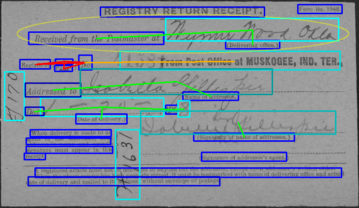
Figure 1: Example label-value relationship pairing. We detect pre-printed text (blue boxes), input text (cyan boxes), and label-value relationships (colored lines) in historical form images. Line colors indicate the correctness of the pairing: true-positive (green), false-negative (orange), or false-positive (red). Note that some relationships are not one-to-one, such as the instance inside the yellow ellipse.

Our method is language-agnostic and does not use text transcriptions, meaning our method can directly be applied to forms in different languages if visual characteristics are the same. While transcriptions may make relationships easier to determine, label-value relationships in forms are typically clear from a purely visual perspective. For example, most people can view a form in an unfamiliar language and infer the label-value relationships. We propose that a deep neural network should be able to infer these relationships as well.

We detect text lines using a Fully Convolutional Network (FCN) as it is effective, simple, and provides features for later processes to reuse. We use a convolutional classifier network to predict which potential relationships are correct using a context window around the relationship. To ensure globally coherent solutions, we predict the number of neighbors for each text line and apply an optimization procedure to find the best set of relationships based on relationship probabilities and the predicted number of neighbors.

Our primary contribution is a trained, end-to-end, language-agnostic method for finding label-value pairs in noisy, novel form images that outperforms heuristic pairing methods. We also show that using dilated, non-square kernels in the FCN text detector improves detection accuracy for long text lines. Finally, we contribute a new annotated dataset of historical form images, the National Archives Forms (NAF) dataset. Our code is at http://github.com/herobd/Visual-Template-Free-Form-Parsing and the NAF dataset is available at http://github.com/herobd/NAF_dataset.

II Previous Work

While a complete solution to the problem of extracting information from forms has many parts (text detection, text recognition, determining the semantic meaning of text, etc.), we review here the aspects most related to our focus, namely detecting and pairing pre-printed and input text.

II-A Text Detection

Older methods for text detection have largely focused on free-form documents, rather than forms and other documents with complex layouts. They have used projection profiles, smearing, or bottom-up methods to identify text lines, all of which must be aware of text regions a priori. They are also not generally resistant to noise. For a survey of these and similar techniques, we refer the interested reader to [1].

Modern approaches have overcome these obstacles using deep learning, presenting solutions that are robust in the presence of noise, arbitrary document layouts, arbitrary orientation, and curved text lines. Grüning et al. [2] use a FCN for pixel labeling followed by post-processing to extract text lines from the pixel predictions. Wigington et al. [3] use a FCN to detect the beginning of text lines and have a network segment the line by stepping along it. Like these methods, we use a FCN, but our method is simpler as it directly predicts bounding rectangles. This limits the types of text lines we can detect (straight, horizontal), but is suitable for our dataset.

II-B Form Processing

Much of the previous work in form processing assumes the availability of templates for form types of interest [4, 5, 6]. This assumption has been relaxed in later work [7, 8]. Zhou et al. [7] assume all relevant information is contained in table structures with lines that can be detected by an OCR engine. Many forms, however, do not have table structures. The method of Hirayama et al. [8] is more general as it allows greater variation in layout. It scores potential labels (pre-printed text) and values (input text) by matching transcribed text with predefined class-dependent dictionaries and rules. Possible relations between text instances are scored using heuristic layout rules. The combination of these two scores define their final pairing score. Hirayama et al. [8] focus on extracting the subset of information from the forms described by the predefined text dictionaries/rules.

Many assumptions made by these methods are broken in our proposed NAF dataset of historical forms. The high noise levels in historical forms can affect the accuracy of classical layout analysis (e.g., line detection). While [8] handles varied layouts, we show that their heuristic layout rules do not generalize well to the NAF dataset.

We are unaware of any publicly available datasets or official reference implementations of prior work that would enable direct comparison with our proposed method.

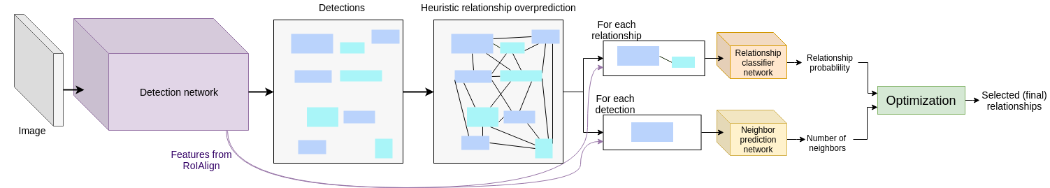
Figure 2: Overview of our method. First we detect pre-printed text and input text lines (shown in more detail in Fig. 4). We then find possible relationships using a line-of-sight heuristic. We then take features from context windows around each detection and each relationship with RoIAlign. These are fed through separate convolutional networks to predict the number of neighbors and the probability of the relationship being true. These predictions are then passed to a global optimization to produce the final relationship predictions.

II-C Scene Graphs

The problem of finding label-value pairs in a form is closely related to the problem of creating scene graphs from natural images, and our proposed method is similar to some previous work in this domain. In scene graphs, the objects in the image are nodes, and edges represent relationships (“on top of”, “is part of”, etc.) between the objects. For our work on forms, pre-printed and input text instances are the objects, and we only consider the label-value relationship.

Zhang et al. [9] use a detection network to predict object and relationship bounding boxes. Then they combine two scores (late fusion) for determining which relationships should be kept. One score is based on learned visual features of object pairs, and the other score is based on spatial features computed from the detected bounding box geometries. We take a similar approach, but perform early fusion of visual and spatial features by inputting them to our network, and we use a heuristic to generate candidate relationships instead of a learned network.

Yang et al. [10] initially only detect and classify objects, but later use a relation-proposal network to predict relationships based on object classes. The proposed relationships are formed into a graph and an attention graph convolution network predicts final relationship and object classes. LinkNet [11] also uses a relation-proposal network and produces object embeddings that are used to find compatible objects for each type of relationship.

III Method Overview

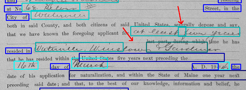
(a) Using normal $3{\times}3$ convolutions

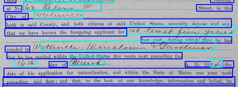
(b) Using dilated $1{\times}3$ convolutions

Figure 3: Detection without dilation (a) and using dilated $1{\times}3$ convolutions (b). Blue boxes are pre-printed text detections, cyan boxes are input text detections. Notice in (a) that long lines are either broken into multiple detections (red arrows) or missed.

An overview of our method to find label-value pairs in form images can be seen in Fig. 2. We detect text/handwriting instances and find possible relationships using a line-of-sight heuristic. For each possible relationship, we extract features from the detection network around the two text instances (padded for context). These features and detection location masks are fed to a small convolutional network to predict the probability of the relationship.

We also perform a global optimization, which takes the predicted probabilities of the relationships and a predicted number of neighbors (number of relationships) per detection and selects which relationships are most in agreement with both of these sets of predictions.

To predict each detection’s number of neighbors, the detector network first predicts an initial estimate. To refine this estimate, we mimic our process of predicting relationships, focusing on a single detection rather than a pair.

IV Detection

We frame the problem of detecting pre-printed text and input text as object detection and use an FCN approach, similar to YOLOv2 [12], to predict text line bounding boxes and classes (pre-printed text or input text). We show that FCNs with dilated $1{\times}3$ convolutions detect long text lines as single entities significantly better than FCNs that use only un-dilated $3{\times}3$ convolutions. We choose to detect text at the line level as this is the input expected by state-of-the-art handwriting recognition methods [13].

For most forms the printed text and handwriting are reasonably horizontal. The primary exception is comments, which are often oriented independently of the document. While work has been done to detect accurate bounding regions for skewed and even curved text [3, 2], we choose a simpler method that is robust to small amounts of skew and assumes straight lines.

Our approach is based on YOLOv2 [12] and uses the loss formulation of YOLOv3 [14]. This model uses a FCN and at each position predicts the probability of objects being present for a number of anchor boxes (prior shapes), how the anchors should be changed to align with the object, and the class of the object.

Using a standard convolutional network (VGG-like) with $3{\times}3$ convolutions yields poor results on long text lines (see Fig. 3a). For a correct detection, information from the ends of the line must propagate to its center (where the prediction is made). Thus the lengths of bounding boxes that can be accurately predicted are limited by the horizontal receptive field of the network. Although many object detection methods [14, 15] use multi-scale approaches, a text line is not at a different scale than the other instances on the page just because it is longer. We instead increase the receptive field horizontally by introducing horizontal dilatation [16]. It can be observed that a $1{\times}3$ convolution followed by a $3{\times}1$ convolution has much of the same effect as a $3{\times}3$ convolution while taking fewer parameters (spatially separable convolution). As we need only the horizontal increase in our receptive field, we use dilated $1{\times}3$ convolutions and non-dilated $3{\times}1$ convolutions. We apply group normalization [17] and ReLU activations between each convolution (we don’t use spatially separable convolution, strictly speaking). Fig. 3 shows a qualitative comparison of results, and Fig. 4 elaborates our architecture.

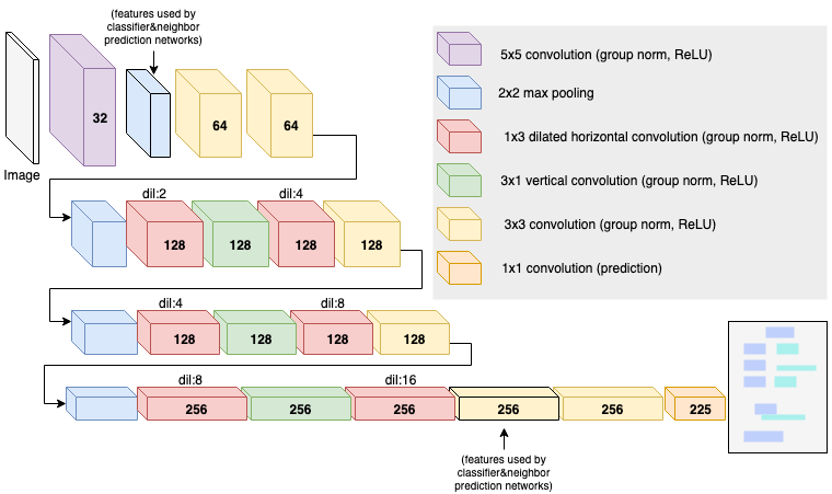
Figure 4: Detector network architecture. Numbers on the boxes are the number of output channels. Dilation amount is indicated above red boxes.

We used 25 anchor boxes found using $k$-nearest neighbors across the ground truth bounding boxes as in [12]. Our seed points were chosen to span the training/validation distribution via manual inspection. The training loss is the same as [14], except we increase a loss weight by 20 to further encourage incorrect detections to have 0 confidence. We found this increases model precision. To prune spurious detections before pairing, we threshold at 0.5 confidence and apply non-maximal suppression.

For our optimization we also have the detector network additionally provide a preliminary prediction of the number of neighbors (relationship pairs) for each detected text. This is done by having the final $1{\times}1$ convolution predict an additional value trained with mean-squared-error loss.

V Pairing

Once we have identified pre-printed text and input text lines, we pair them to find label-value relationships. First, we identify a high-recall list of potential relationships using a simple heuristic. Then, we extract features for each candidate relationship and predict how likely those elements are to be related. Finally, because there can be local ambiguity, we use these pairwise scores in a global optimization to derive the final set of relationships.

V-A Identifying Candidate Relationships

We first identify candidate relationships from the detection results to reduce computation compared to exploring all possible detection pairs. All pairs of bounding boxes whose edges are within line-of-sight of each other, and are not too far away from each other, are considered candidates. The line-of-sight is determined by tracing rays from points along the edges of bounding boxes which terminate after entering a bounding box (see Fig. 5). To address memory limitations during training, the combined number of candidates and relationships is limited to a pre-determined maximum (set to 370 in our implementation). If the number exceeds the threshold, the maximum length of the rays is shortened and the process is repeated. This heuristic has 96.6% recall for the test set relationships.

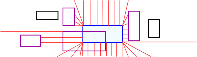
Figure 5: Heuristic relationship overprediction is done using line-of-sight. The red lines are the rays determining the line-of-sight of the blue box. Purple boxes are pairing candidates for the blue box.

V-B Classifying Candidate Relationships

Many forms place labels to the left of their corresponding value, though sometimes the label may be above or below the value. A prior work [8] attempted to leverage regularity of form layouts by hand-crafting heuristic rules to score potential relationships, but hand-tuned scoring functions can fail in the template-free case when form layouts do not always match the assumptions made by the heuristic. A more generalizable approach is to learn implicit rules by training on a variety of different form layouts. We use the following features when pairing two element bounding boxes:

• Difference of center $x$ and $y$ positions

• Distance from each corner to its counterpart (top-left to top-left, bottom-left to bottom-left, etc.)

• Normalized height and width of each bounding box (divided by 50 and 400, respectively)

• Detector predicted probabilities of belonging to the pre-printed text / input text classes for both bounding boxes

• Predicted number of neighbors for each bounding box

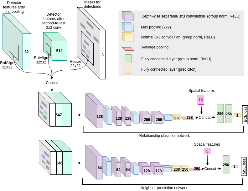
Figure 6: Relationship classifier and neighbor prediction networks. Numbers on the boxes indicate the number of output channels. Both networks receive as input the concatenation of the detector’s first pooling layer and second-to-last convolution layer (extracted with RoIAlign [18]), as well as resized detection masks. The relationship classifier predicts the probability that the two input detections have a relationship. The neighbor prediction network refines the prediction of the number of neighbors for the input detection. We use depth-wise separable convolution to reduce the number of parameters [19].

It is clear that, in addition to spatial features, humans also use multiple visual cues in determining relationships: lines, borders, nearby text and handwriting, etc. To allow for the learning of these cues, we also use a convolutional network to analyze the area surrounding each potential pairing.

For each candidate relationship we find the rectangular area bounding the two bounding box detections and pad it by 150 pixels on each side to provide local context. We append detector network features from both the second-to-last convolution layer and the first pooling layer. These features are cropped with RoIAlign [18] to the size $32{\times}32$. We append three additional binary masks to these features (resized to $32{\times}32$), one mask for each bounding box in the candidate relationship and a mask of all detected bounding boxes (Fig. 6, top left). The input order of the candidate text bounding box masks are randomized during training. For evaluation we average the result of both orderings.

We extract features from this input tensor with a small convolutional network and apply global pooling to the resulting features. The resulting flattened features are appended to the previously described spatial features, and a fully connected network classifies the candidate relationship as valid or not. This network is trained with a binary cross-entropy loss. Fig. 6 shows the pairing network architecture.

VI Neighbor Prediction Network

For the subsequent global optimization (Section VII), we predict the number of neighbors (relationships) each detected printed/input text element has. While the detection network makes initial predictions, better predictions can be made after removing spurious predictions and by focusing on each individual text detection.

We apply another small convolutional network (Fig. 6) to the region around each detection, in a similar manner as described in Section V-B. However, this network has only two input masks: one for the detection of interest and one for all detections. The features appended before the fully-connected layers are also slightly different: normalized height and width, initially predicted number of neighbors, and class prediction.

TABLE I: NAF Dataset characteristics

Version	Split	Images	# Form Types	Pre-printed Text	Input Text	Label-Value relationships
Simple	Train	143	51	4547	2589	2496
	Validation	11	6	368	162	159
	Test	11	8	250	189	161
Full	Train	682	209	40347	12482	-
	Validation	59	31	3381	1266	-
	Test	63	34	2892	1229	-

VII Global Optimization

The problem of determining a single relationship can depend on other relationship decisions for a form. Imagine the scenario where a pre-printed text line has an equal probability to be in a relationship with two different handwriting instances, but one of the handwriting instances has another possible pairing and the other does not. Assuming we know each of these handwriting instances should be paired with only one pre-printed text instance, we can easily recognize the appropriate pairings for them. To take all relationship decisions into account at once we employ global optimization as a post-processing step.

Ideally, we want to encourage the number of predicted relationships per bounding box to be similar to the predicted number of neighbors for each detected element, while respecting the probability or score of the relationships.

Let $R$ be the set of candidate relationships and $\mathbf{x}$ be a vector of binary labels, such that $x_{r}=1$ indicates that relationship $r\in R$ is accepted. Let $p_{r}$ be the pairing network’s predicted probability for $r$, $n_{b}\in\mathbb{R}$ be the estimated number of neighbors for the detected bounding box $b\in B$, and $R_{b}\subseteq R$ be the subset of all relationships that $b$ is part of. The tune-able parameter $c$ determines how much confidence we place in the accuracy of $n_{b}$, and $T$ is a (soft) threshold. We formulate our optimization as

$$\mathbf{x^{*}}\!=\!\underset{\mathbf{x}}{\text{argmax}}\!\left[\sum\limits_{r\in R}(p_{r}\!-T)x_{r}\!-c\sum\limits_{b\in B}\big{(}n_{b}-\!\!\sum\limits_{r\in R_{b}}x_{r}\big{)}^{2}\right]$$ (1)

The first term of Eq. 1 seeks to reject relationships with probabilities less than $T$. With $c=0$, Eq. 1 reduces to thresholding with $p_{r}\geq T$. The second term regularizes each $b$ to have $n_{b}$ neighbors. To handle uncertainty, $n_{b}$ can be a non-integer. For example, if $b$ could have 0 or 1 neighbors, having $n_{b}=0.5$ equally penalizes both cases. We found $c=0.25$ and $T=0.7$ worked well on the validation set for most experiments and used this in our evaluation. We use the branch-and-bound variant of ECOS [20] to solve Eq. 1.

VIII NAF Dataset

We introduce and release a new dataset of annotated historical form images, the National Archives Forms (NAF) dataset, with the following properties:

• Varied form layouts, with train, validation, and test sets having disjoint form layouts.

• Historical, noisy.

• Filled in by hand and/or typewriter.

The NAF dataset is comprised of historical form images from the United States National Archives. The images are noisy due to degradation and the machinery used to print them. Figures 1, 3, and 7 contain examples from the dataset.

We have restricted our pairing dataset to images not containing tables or prose/fill-in-the-blank information in order to focus on the label-value problem (other approaches will be more effective for these types of forms). However, we use the full dataset for pre-training the detection network.

We divided the images into training, validation, and test sets, where each set has a distinct set of form layouts, though there are multiple instances of each form layout within each set. This mimics the template-free scenario, i.e., we test on form layouts our system has never seen before. Details of this dataset can be seen in Table  I.

Elements of the images are annotated with quadrilaterals, which we convert to axis-aligned rectangles. For this work, we use only the pre-printed text and input text annotations, though the dataset does contain richer annotations. We use only the relationships between pre-printed text and input text elements as these typically are label-value relationships.

IX Experiments and Results

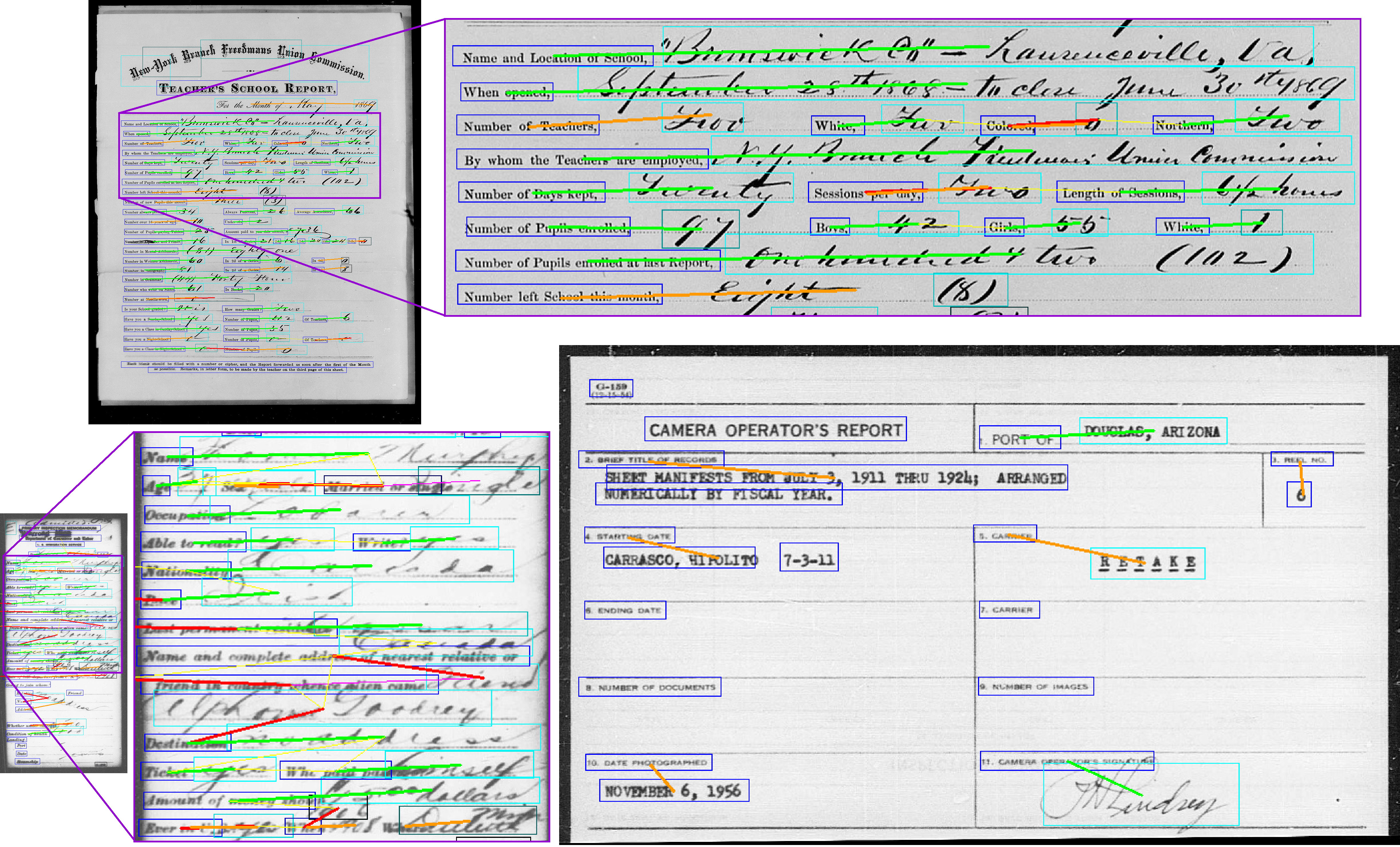
Figure 7: Test set examples. Blue and cyan boxes are pre-printed text and input text detections respectively. Green lines are correct relationship predictions, red lines are false positive errors, orange lines are false negative errors, thin yellow lines are relationships correctly pruned by the optimization, thin pink lines are relationships incorrectly pruned by the optimization. The relationship AP of the images: top-left 0.625, bottom-left 0.503, bottom-right 0.371

IX-A Training

We train all our models with the Adam optimizer  [21] and used the validation set to determine hyper-parameters.

For both detection and pairing, we uniformly randomly resize training images to 0.4–0.65 of their original size. A training instance is a random $652{\times}1608$ crop of the resized image. This size captures several complete relationships while using less memory than a full image. If a text instance is cropped horizontally, we clip its bounding box to fit in the window. If a text instance is cropped vertically so that less than half the bounding box is inside the window, we remove the instance from the ground truth. For data augmentation, we also randomly perturb contrast as in [3].

For detection: We use the full dataset for training the detector network. We apply additional data augmentation when training the detection network by randomly rotating images slightly and flipping them horizontally. We use a learning rate of 0.01 and a batch size of 5. We pre-train the detector network to 150,000 iterations.

For pairing: We use a subset of the dataset as described in Section VIII. The detector network is frozen for the first 2,000 iterations and afterwards its weights are fine-tuned through all tasks’ losses. At each training iteration for the pairing network we present either predicted or ground-truth bounding boxes. The probability of using ground truth bounding boxes is initially 100% and then lowered until it reaches 50% at 20,000 iterations. We use an IoU threshold of 0.4 in aligning predicted and ground truth bounding boxes to determine which predicted relationships are true. We threshold detections at 0.5 IoU. If a predicted bounding box does not overlap with any ground truth, all possible relationships with it are false. If a prediction overlaps with ground truth by less than the IoU threshold, we do not calculate the loss for its relationships that would be true. We use a learning schedule similar to [22] with a warm-up of 1,000 iterations, a maximum learning rate of 0.0015 and a mean learning rate of 0.00062 . The batch size is 1. We terminate training at 125,000 iterations. We weight the multiple loss terms as follows, detection: 1.0, pairing: 0.5, and number of neighbor regression: 0.25.

IX-B Evaluation

Qualitative detection and pairing results for images from the test set can be seen in Fig. 7. It can be observed in the top image crop and bottom-left image crop that the optimization removes several false-positive relationships which are not consistent with neighboring predictions (thin yellow lines). In the bottom-right image the detector struggles to correctly predict the class of input text that is printed, and thus misses several relationships. Other observations we made of the results are that the model struggles with predicting long distance relationships, and continues to have errors where multiple relationships are plausible, even after optimization. For many errors it is unclear what the cause is, e.g. the model predicts the correct number of neighbors for two detections that should be paired, but predicts a low probability of pairing them in the absence of obvious distractors.

For quantitative evaluation we measure mean average precision (mAP), recall, precision, and F-measure (F-m) for both detection and relationship predictions. For a text detection to be correct it must have at least 0.5 IOU with a GT bounding box and match the GT class. For a predicted relationship to be correct it must be between two correct detections whose matched GTs have a relationship.

TABLE II: Detection results

		Pairing dataset						Full dataset
			avg.	pre-printed text		input text			avg.
Method	# params	mAP	F-m	prec.	recall	prec.	recall	mAP	F-m
Standard ConvNet (VGG-like)	3M	0.364	0.719	0.811	0.780	0.689	0.603	0.324	0.612
Dilated staggered convs (Fig. 4) pre-trained	2.4M	0.423	0.836	0.861	0.908	0.816	0.763	0.421	0.808
Dilated staggered convs (Fig. 4) fine-tuned	2.4M	0.428	0.795	0.791	0.906	0.726	0.768	-	-

TABLE III: Pairing results

	Without optimization				After global optimization
Method	mAP	F-m	prec.	recall	mAP	F-m	prec.	recall
Distance based	0.235	0.217	0.134	0.666	0.251	0.306	0.254	0.428
Scoring functions from [8]	0.135	0.063	0.162	0.080	0.136	0.077	0.151	0.086
Classifier w/o visual features	0.248	0.240	0.157	0.680	0.275	0.352	0.277	0.516
ConvNet with visual features	0.585	0.589	0.559	0.655	0.584	0.607	0.654	0.599

TABLE IV: Upper bound experiments using perfect information

	optimized		using GT
	w/ GT NN		detections
Method	mAP	F-m	mAP	F-m
Distance based	0.413	0.504	0.424	0.314
Scoring functions from [8]	0.136	0.073	0.238	0.085
Classifier w/o visual features	0.509	0.597	0.428	0.377
ConvNet with visual features	0.640	0.721	0.912	0.855

Average precision (AP) requires continuous scores, so when we optimize we subtract 1 from the probability of each rejected relationship to maintain order before calculating AP. For F-m, recall, and precision we threshold the detector at 0.5, and we threshold pairing at 0.5 ($T{=}0.5$ for optimization).

We first compare our detection network architecture to a standard convolutional (VGG-like) network that does not use dilation. Table II shows the number of parameters in each model and their respective performance on the full test set (average of five different training runs). While the dilated architecture we propose has fewer parameters, it significantly outperforms the standard convolutional network.

To demonstrate that the proposed learning-based pairing method outperforms simple heuristics, we implemented two baseline methods based on heuristic rules. The first is a simple one based on inverse distance (i.e. closer elements of opposite classes are more likely to be paired):

$$s_{i,j}=1-\frac{\left\|(x_{i},y_{i})-(x_{j},y_{j})\right\|-d_{min}}{d_{max}-d_{min}}$$ (2)

where $(x_{i},y_{i})$ and $(x_{j},y_{j})$ are the centers of the bounding boxes for two detected text elements of different class, and $d_{max}$ and $d_{min}$ are the maximum and minimum distances for all potential relationships. The second baseline uses a scoring function adapted from [8]. They use cell boundaries (of field areas) in some of their scoring terms, which we cannot use, so we use only the scoring terms based on height, distance, and whether the value is to the right of the label. Intuitively, the scoring penalizes pairing text elements of different heights, distantly separated text elements, and input text to the right of the pre-printed text.

To evaluate the additive effect of using visual cues in addition to spatial features, we implemented a baseline network that takes as input only the spatial features listed in Section V-B and not the contextual visual features our full method does. For this classifier we use three fully connected layers with batch normalization, dropout, and ReLU activations for the first 2 layers. We use a hidden size of 256. We trained the network with a binary cross-entropy loss, a learning rate of 0.001, and a batch size of 512 for 6,000 iterations.

The performance of our proposed method compared to these baseline methods is shown in Table III (average of 5 training runs). Surprisingly the distance-based method’s performance is similar to the non-visual classifier. Including visual features significantly outperforms any of the baselines. The global optimization improves F-measure as it sacrifices some recall for greater precision. The gains are more evident with the distance-based heuristic and the non-visual classifier. Our model sees a context window and so can already reason about neighbors without the optimization.

IX-C Additional Experiments

As seen in Table IV (average of five training runs), substituting the ground-truth number of neighbors during the optimization instead of the predicted number (and using $c=25$) greatly increases the effectiveness of the optimization.

Because this work focuses on pairing form elements, we also evaluate the upper-bound performance of our proposed and baseline pairing methods by using ground truth text detections instead of predicted ones (Table IV, average of five training runs). This allows us to examine the performance of the pairing network independent of the means of detection. The number of neighbors is part of the detection ground truth; to minimize this information’s impact we introduce a $\pm 1$ uniform noise to the number of neighbors. As expected, all of the methods improve when given perfect detections as input.

We also measured the contribution made by the neighbor prediction network, which refines the predicted number of neighbors after the initial detection network. The neighbor prediction network predicts the number of neighbors with 72% accuracy, while the detector alone predicts the number of neighbors with 50% accuracy, suggesting that the use of this auxiliary network is helpful.

X Conclusion

We have introduced a trainable, language-agnostic method to detect and pair pre-printed text and input text in form images that is robust to noise found in historical documents. We have also introduced the NAF dataset, which contains images of historical forms with a variety of layouts, and evaluated our method against alternative baselines using this dataset. There is not an existing benchmark for this problem.

The results presented here show that dilated $1{\times}3$ convolutions make a FCN more effective at detecting long text lines. These results also indicate that having a learned method that uses visual features is important when pairing text lines. We have also found that optimizing results across a page leads to increased precision.

References

- [1] L. Likforman-Sulem, A. Zahour, and B. Taconet, “Text line segmentation of historical documents: a survey,” International Journal of Document Analysis and Recognition, vol. 9, no. 2-4, pp. 123–138, 2007.
- [2] T. Grüning, G. Leifert, T. Strauß, and R. Labahn, “A two-stage method for text line detection in historical documents,” arXiv preprint arXiv:1802.03345, 2018.
- [3] C. Wigington, C. Tensmeyer, B. Davis, W. Barrett, B. Price, and S. Cohen, “Start, follow, read: End-to-end full-page handwriting recognition,” in European Conference on Computer Vision (ECCV), 2018, pp. 367–383.
- [4] W. Barrett, L. Hutchison, D. Quass, H. Nielson, and D. Kennard, “Digital mountain: From granite archive to global access,” in International Workshop on Document Image Analysis for Libraries, 2004, pp. 104–121.
- [5] M. A. Butt, “Information extraction from pre-preprinted documents,” International Journal of Computers and Distributed System, vol. 2, no. 1, pp. 88–93, 2012.
- [6] M. Hammami, P. Héroux, S. Adam, and V. P. d’Andecy, “One-shot field spotting on colored forms using subgraph isomorphism,” in International Conference on Document Analysis and Recognition (ICDAR), 2015.
- [7] J. Zhou, H. Yu, C. Xie, H. Cai, and L. Jiang, “iRMP: From printed forms to relational data model,” in IEEE HPCC/SmartCity/DSS, 2016, pp. 1394–1401.
- [8] J. Hirayama, H. Shinjo, T. Takahashi, and T. Nagasaki, “Development of template-free form recognition system,” in International Conference on Document Analysis and Recognition (ICDAR), 2011, pp. 237–241.
- [9] J. Zhang, M. Elhoseiny, S. Cohen, W. Chang, and A. Elgammal, “Relationship proposal networks,” in IEEE Computer Vision and Pattern Recognition (CVPR), vol. 1, 2017, p. 2.
- [10] J. Yang, J. Lu, S. Lee, D. Batra, and D. Parikh, “Graph R-CNN for scene graph generation,” in European Conference on Computer Vision (ECCV), 2018, pp. 670–685.
- [11] S. Woo, D. Kim, D. Cho, and I. S. Kweon, “LinkNet: Relational embedding for scene graph,” in Advances in Neural Information Processing Systems, 2018, pp. 558–568.
- [12] J. Redmon and A. Farhadi, “YOLO9000: better, faster, stronger,” in IEEE Computer Vision and Pattern Recognition (CVPR), 2017, pp. 7263–7271.
- [13] J. Puigcerver, “Are multidimensional recurrent layers really necessary for handwritten text recognition?” in International Conference on Document Analysis and Recognition (ICDAR), vol. 1, 2017, pp. 67–72.
- [14] J. Redmon and A. Farhadi, “YOLOv3: An incremental improvement,” arXiv preprint arXiv:1804.02767, 2018.
- [15] R. Girshick, “Fast R-CNN,” in IEEE International Conference on Computer Vision (ICCV), December 2015.
- [16] A. van den Oord, S. Dieleman, H. Zen, K. Simonyan, O. Vinyals, A. Graves, N. Kalchbrenner, A. W. Senior, and K. Kavukcuoglu, “Wavenet: A generative model for raw audio,” in ISCA Speech Synthesis Workshop (SSW), 2016.
- [17] Y. Wu and K. He, “Group normalization,” in European Conference on Computer Vision, 2018, pp. 3–19.
- [18] K. He, G. Gkioxari, P. Dollár, and R. Girshick, “Mask R-CNN,” in IEEE International Conference on Computer Vision (ICCV), 2017, pp. 2961–2969.
- [19] A. G. Howard, M. Zhu, B. Chen, D. Kalenichenko, W. Wang, T. Weyand, M. Andreetto, and H. Adam, “Mobilenets: Efficient convolutional neural networks for mobile vision applications,” arXiv preprint arXiv:1704.04861, 2017.
- [20] A. Domahidi, E. Chu, and S. Boyd, “ECOS: An SOCP solver for embedded systems,” in European Control Conference, 2013, pp. 3071–3076.
- [21] D. P. Kingma and J. Ba, “Adam: A method for stochastic optimization,” arXiv preprint arXiv:1412.6980, 2014.
- [22] A. Vaswani, N. Shazeer, N. Parmar, J. Uszkoreit, L. Jones, A. N. Gomez, Ł. Kaiser, and I. Polosukhin, “Attention is all you need,” in Advances in Neural Information Processing Systems, 2017, pp. 5998–6008.