Number of Sign Changes: Segment of AR(1)

Abstract

Let $X_{t}$ denote a stationary first-order autoregressive process.  Consider $n$ contiguous observations (in time $t$) of the series (e.g., $X_{1}$, …, $X_{n}$). Let its mean be zero and its lag-one serial correlation be $\rho$, which satisfies $\left|\rho\right|<1$.  Rice (1945) proved that $(n-1)\arccos(\rho)/\pi$ is the expected number of sign changes.  A corresponding formula for higher-order moments was proposed by Nyberg, Lizana & Ambjörnsson (2018), based on an independent interval approximation.  We focus on the variance only, for small $n$, and see a promising fit between theory and model.

Given

$$\begin{array}[c]{ccccc}X_{t}=\rho\,X_{t-1}+\sqrt{1-\rho^{2}}\cdot\varepsilon_{t},&&-\infty<t<\infty,&&|\rho|<1\end{array}$$

where $\varepsilon_{t}$ is $N(0,1)$ white noise, the segment $(X_{1},\ldots,X_{n})$ is Gaussian with vector mean and covariance matrix

$$R=\left(\begin{array}[c]{ccccccc}1&\rho&\rho^{2}&\ldots&\rho^{n-3}&\rho^{n-2}&\rho^{n-1}\\ \rho&1&\rho&\ldots&&\rho^{n-3}&\rho^{n-2}\\ \rho^{2}&\rho&1&&\ldots&&\rho^{n-3}\\ \vdots&\vdots&&\ddots&\ddots&\vdots&\vdots\\ \rho^{n-3}&&\vdots&\ddots&1&\rho&\rho^{2}\\ \rho^{n-2}&\rho^{n-3}&&\ldots&\rho&1&\rho\\ \rho^{n-1}&\rho^{n-2}&\rho^{n-3}&\ldots&\rho^{2}&\rho&1\end{array}\right).$$

In particular, all variances are one and the correlation between $X_{i}$ and $X_{j}$ is $\rho^{\left|j-i\right|}$.  Define $S_{n}=\#\{i:1\leq i<n$ and $X_{i}X_{i+1}<0\}$, the number of sign changes, and

$$p_{e}(R)=\mathbb{P}\left\{(-1)^{e_{1}}X_{1}<0\text{, \ }(-1)^{e_{2}}X_{2}<0\text{, \ldots, }(-1)^{e_{n-1}}X_{n-1}<0\text{ and }(-1)^{e_{n}}X_{n}<0\right\}$$

for any vector $e$ of $n$ bits.  It is well known that [1, 2, 3, 4, 5]

$$p_{11} =\mathbb{P}\left\{X_{1}>0\text{ and }X_{2}>0\right\}$$

$$=\frac{1}{4}+\frac{1}{2\pi}\arcsin\left(\rho\right)$$

$$=\mathbb{P}\left\{X_{1}<0\text{ and }X_{2}<0\right\}=p_{00}$$

and

$$p_{111} =\mathbb{P}\left\{X_{1}>0\text{, }X_{2}>0\text{ and }X_{3}>0\right\}$$

$$=\frac{1}{8}+\frac{1}{4\pi}\left[\arcsin\left(\rho\right)+\arcsin\left(\rho^{2}\right)+\arcsin\left(\rho\right)\right]$$

$$=\mathbb{P}\left\{X_{1}<0\text{, }X_{2}<0\text{ and }X_{3}<0\right\}=p_{000}.$$

Because

$$\operatorname{Cov}\left(\begin{array}[c]{c}-X_{1}\\ X_{2}\end{array}\right)=\left(\begin{array}[c]{cc}1&-\rho\\ -\rho&1\end{array}\right),$$

we have

$$p_{10} =\mathbb{P}\left\{X_{1}>0\text{ and }X_{2}<0\right\}$$

$$=\frac{1}{4}-\frac{1}{2\pi}\arcsin\left(\rho\right)$$

$$=\mathbb{P}\left\{X_{1}<0\text{ and }X_{2}>0\right\}=p_{01}$$

and hence

$$\mathbb{E}\left(S_{2}\right)=2p_{10}=\frac{1}{2}-\frac{1}{\pi}\arcsin\left(\rho\right)=\frac{1}{\pi}\left[\frac{\pi}{2}-\arcsin\left(\rho\right)\right]=\frac{\arccos(\rho)}{\pi},$$

$$\mathbb{V}\left(S_{2}\right) =2p_{10}-\left(2p_{10}\right)^{2}=2p_{10}\left(1-2p_{10}\right)=\left[\frac{1}{2}-\frac{1}{\pi}\arcsin\left(\rho\right)\right]\left[\frac{1}{2}+\frac{1}{\pi}\arcsin\left(\rho\right)\right]$$

$$=\frac{1}{4}-\frac{1}{\pi^{2}}\arcsin\left(\rho\right)^{2}.$$

Because

$$\operatorname{Cov}\left(\begin{array}[c]{c}-X_{1}\\ X_{2}\\ X_{3}\end{array}\right)=\left(\begin{array}[c]{ccc}1&-\rho&-\rho^{2}\\ -\rho&1&\rho\\ -\rho^{2}&\rho&1\end{array}\right)$$

and

$$\operatorname{Cov}\left(\begin{array}[c]{c}X_{1}\\ X_{2}\\ -X_{3}\end{array}\right)=\left(\begin{array}[c]{ccc}1&\rho&-\rho^{2}\\ \rho&1&-\rho\\ -\rho^{2}&-\rho&1\end{array}\right)$$

we have

$$p_{100} =p_{011}=\frac{1}{8}+\frac{1}{4\pi}\left[-\arcsin\left(\rho\right)-\arcsin\left(\rho^{2}\right)+\arcsin\left(\rho\right)\right]$$

$$=p_{001}=p_{110};$$

because

$$\operatorname{Cov}\left(\begin{array}[c]{c}X_{1}\\ -X_{2}\\ X_{3}\end{array}\right)=\left(\begin{array}[c]{ccc}1&-\rho&\rho^{2}\\ -\rho&1&-\rho\\ \rho^{2}&-\rho&1\end{array}\right)$$

we have

$$p_{010}=p_{101}=\frac{1}{8}+\frac{1}{4\pi}\left[-\arcsin\left(\rho\right)+\arcsin\left(\rho^{2}\right)-\arcsin\left(\rho\right)\right];$$

thus

$$\mathbb{E}\left(S_{3}\right) =4p_{100}+2\cdot 2p_{010}$$

$$=\frac{1}{2}-\frac{1}{\pi}\arcsin\left(\rho^{2}\right)+\frac{1}{2}+\frac{1}{\pi}\left[-2\arcsin\left(\rho\right)+\arcsin\left(\rho^{2}\right)\right]$$

$$=\frac{2}{\pi}\left[\frac{\pi}{2}-\arcsin\left(\rho\right)\right]=\frac{2\arccos(\rho)}{\pi},$$

$$\mathbb{V}\left(S_{3}\right) =4p_{100}+2\cdot 4p_{010}-\left(4p_{100}+2\cdot 2p_{010}\right)^{2}$$

$$=\frac{1}{2}-\frac{1}{\pi}\arcsin\left(\rho^{2}\right)+1+\frac{2}{\pi}\left[-2\arcsin\left(\rho\right)+\arcsin\left(\rho^{2}\right)\right]-\left[1-\frac{2}{\pi}\arcsin\left(\rho\right)\right]^{2}$$

$$=\frac{3}{2}-\frac{4}{\pi}\arcsin\left(\rho\right)+\frac{1}{\pi}\arcsin\left(\rho^{2}\right)-1+\frac{4}{\pi}\arcsin\left(\rho\right)-\frac{4}{\pi^{2}}\arcsin\left(\rho\right)^{2}$$

$$=\frac{1}{2}-\frac{4}{\pi^{2}}\arcsin\left(\rho\right)^{2}+\frac{1}{\pi}\arcsin\left(\rho^{2}\right).$$

These formulas are consistent with a distributional result $S_{n}\sim\operatorname{Binomial}(n-1,1/2)$ valid when observations are independent; in particular,

$$\begin{array}[c]{ccc}\mathbb{E}\left(S_{n}\right)=\dfrac{n-1}{2},&&\mathbb{V}\left(S_{n}\right)=\dfrac{n-1}{4}\end{array}$$

for $\rho=0$.  The case $n=4$ for $\rho\neq 0$ is more difficult and will be covered in the next section.  Closed-form variance expressions become impossible for $n\geq 5$ (see the appendix) and a certain approximative model shall occupy us for the remainder of this paper.

1 Dilogarithm Formula

Cheng [6, 7, 8, 9] evaluated the following integral:

$$I(h,x)={\displaystyle\int\limits_{0}^{x}}\arcsin\left(\frac{\left(1-h^{2}\right)t}{h^{2}-t^{2}}\right)\frac{1}{\sqrt{1-t^{2}}}\,dt$$

to be:

$$-\frac{1}{2}\arcsin(x)^{2}+\frac{1}{2}\operatorname{Li}_{2}\left[-\frac{\left(h^{2}-\sqrt{h^{4}-x^{2}}\right)^{2}}{x^{2}}\right]$$

$$+\operatorname{Li}_{2}\left[\frac{\left(x-i\sqrt{1-x^{2}}\right)\left(h^{2}-\sqrt{h^{4}-x^{2}}\right)}{x}\right]+\operatorname{Li}_{2}\left[\frac{\left(x+i\sqrt{1-x^{2}}\right)\left(h^{2}-\sqrt{h^{4}-x^{2}}\right)}{x}\right]$$

$$-\frac{1}{2}\operatorname{Li}_{2}\left[\frac{\left(h^{2}-i\sqrt{1-h^{2}}\right)^{2}\left(h^{2}-\sqrt{h^{4}-x^{2}}\right)^{2}}{x^{2}}\right]-\frac{1}{2}\operatorname{Li}_{2}\left[\frac{\left(h^{2}+i\sqrt{1-h^{2}}\right)^{2}\left(h^{2}-\sqrt{h^{4}-x^{2}}\right)^{2}}{x^{2}}\right]$$

where $0<x<h^{2}<1$ and $\operatorname{Li}_{2}[z]$ is the complex dilogarithm function. Associated with covariance matrix

$$R^{+}=\left(\begin{array}[c]{cccc}1&a&ab&a^{2}b\\ a&1&b&ab\\ ab&b&1&a\\ a^{2}b&ab&a&1\end{array}\right)$$

is orthant probability

$$p_{1111}(R^{+})=\frac{1}{16}+\frac{2\arcsin(a)+\arcsin(b)+2\arcsin(ab)+\arcsin\left(a^{2}b\right)}{8\pi}+\frac{\arcsin(a)^{2}+I(a,a^{2}b)}{4\pi^{2}};$$

call this $f(a,b)$.  Associated with covariance matrix

$$R^{-}=\left(\begin{array}[c]{cccc}1&-a&-ab&-a^{2}b\\ -a&1&b&ab\\ -ab&b&1&a\\ -a^{2}b&ab&a&1\end{array}\right)$$

is orthant probability

$$p_{1111}(R^{-})=\frac{1}{16}+\frac{\arcsin(b)-\arcsin\left(a^{2}b\right)}{8\pi}-\frac{\arcsin(a)^{2}+I(a,a^{2}b)}{4\pi^{2}};$$

call this $g(a,b)$.  We assume that $\left|a\right|<1$ and $\left|b\right|<1$.  Note that the matrix elements $R_{12}^{+}$ and $R_{34}^{+}$ are identical, whereas $R_{12}^{-}$ and $R_{34}^{-}$ are of opposite sign.  Let us now return to our original $4\times 4$ matrix $R$.  Clearly

$$p_{1111} =\mathbb{P}\left\{X_{1}>0\text{, }X_{2}>0\text{, }X_{3}>0\text{ and }X_{4}>0\right\}$$

$$=f(\rho,\rho)$$

$$=\mathbb{P}\left\{X_{1}<0\text{, }X_{2}<0\text{, }X_{3}<0\text{ and }X_{4}<0\right\}=p_{0000}.$$

Because

$$\operatorname{Cov}\left(\begin{array}[c]{c}-X_{1}\\ X_{2}\\ X_{3}\\ X_{4}\end{array}\right)=\left(\begin{array}[c]{cccc}1&-\rho&-\rho^{2}&-\rho^{3}\\ -\rho&1&\rho&\rho^{2}\\ -\rho^{2}&\rho&1&\rho\\ -\rho^{3}&\rho^{2}&\rho&1\end{array}\right)$$

and

$$\operatorname{Cov}\left(\begin{array}[c]{c}X_{1}\\ X_{2}\\ X_{3}\\ -X_{4}\end{array}\right)=\left(\begin{array}[c]{cccc}1&\rho&\rho^{2}&-\rho^{3}\\ \rho&1&\rho&-\rho^{2}\\ \rho^{2}&\rho&1&-\rho\\ -\rho^{3}&-\rho^{2}&-\rho&1\end{array}\right)$$

we have

$$p_{1000} =p_{0111}=g(\rho,\rho)$$

$$=g(-\rho,\rho)=p_{0001}=p_{1110};$$

because

$$\operatorname{Cov}\left(\begin{array}[c]{c}X_{1}\\ -X_{2}\\ X_{3}\\ X_{4}\end{array}\right)=\left(\begin{array}[c]{cccc}1&-\rho&\rho^{2}&\rho^{3}\\ -\rho&1&-\rho&-\rho^{2}\\ \rho^{2}&-\rho&1&\rho\\ \rho^{3}&-\rho^{2}&\rho&1\end{array}\right)$$

and

$$\operatorname{Cov}\left(\begin{array}[c]{c}X_{1}\\ X_{2}\\ -X_{3}\\ X_{4}\end{array}\right)=\left(\begin{array}[c]{cccc}1&\rho&-\rho^{2}&\rho^{3}\\ \rho&1&-\rho&\rho^{2}\\ -\rho^{2}&-\rho&1&-\rho\\ \rho^{3}&\rho^{2}&-\rho&1\end{array}\right)$$

we have

$$p_{0100} =p_{1011}=g(\rho,-\rho)$$

$$=g(-\rho,-\rho)=p_{0010}=p_{1101}.$$

Because

$$\operatorname{Cov}\left(\begin{array}[c]{c}-X_{1}\\ -X_{2}\\ X_{3}\\ X_{4}\end{array}\right)=\left(\begin{array}[c]{cccc}1&\rho&-\rho^{2}&-\rho^{3}\\ \rho&1&-\rho&-\rho^{2}\\ -\rho^{2}&-\rho&1&\rho\\ -\rho^{3}&-\rho^{2}&\rho&1\end{array}\right)$$

we have

$$p_{1100}=p_{0011}=f(\rho,-\rho);$$

because

$$\operatorname{Cov}\left(\begin{array}[c]{c}X_{1}\\ -X_{2}\\ -X_{3}\\ X_{4}\end{array}\right)=\left(\begin{array}[c]{cccc}1&-\rho&-\rho^{2}&\rho^{3}\\ -\rho&1&\rho&-\rho^{2}\\ -\rho^{2}&\rho&1&-\rho\\ \rho^{3}&-\rho^{2}&-\rho&1\end{array}\right)$$

we have

$$p_{0110}=p_{1001}=f(-\rho,\rho);$$

because

$$\operatorname{Cov}\left(\begin{array}[c]{c}-X_{1}\\ X_{2}\\ -X_{3}\\ X_{4}\end{array}\right)=\left(\begin{array}[c]{cccc}1&-\rho&\rho^{2}&-\rho^{3}\\ -\rho&1&-\rho&\rho^{2}\\ \rho^{2}&-\rho&1&-\rho\\ -\rho^{3}&\rho^{2}&-\rho&1\end{array}\right)$$

we have

$$p_{1010}=p_{0101}=f(-\rho,-\rho).$$

Thus

$$\mathbb{E}\left(S_{4}\right) =4p_{1000}+2p_{1100}+4\cdot 2p_{0100}+2\cdot 2p_{0110}+2\cdot 3p_{1010}$$

$$=4g(\rho,\rho)+2f(\rho,-\rho)+8g(\rho,-\rho)+4f(-\rho,\rho)+6f(-\rho,-\rho)$$

$$=\frac{3\arccos(\rho)}{\pi},$$

$$\mathbb{V}\left(S_{4}\right) =4p_{1000}+2p_{1100}+4\cdot 4p_{0100}+2\cdot 4p_{0110}+2\cdot 9p_{1010}-\left(3\arccos(\rho)/\pi\right)^{2}$$

$$=4g(\rho,\rho)+2f(\rho,-\rho)+16g(\rho,-\rho)+8f(-\rho,\rho)+18f(-\rho,-\rho)-9\left[1/2-\arcsin(\rho)/\pi\right]^{2}.$$

Unlike the mean, our expression for the variance does not simplify appreciably.  A plot of $\mathbb{V}\left(S_{4}\right)$ falls off symmetrically from both sides of the maximum value $3/4$ at $\rho=0$.  For specificity’s sake, we indicate numerical values at $\rho=1/2$:

$$\begin{array}[c]{ll}f(1/2,1/2)=&0.1576625817544825416159596...,\\ g(1/2,1/2)=&0.0707784073926423526601112...,\\ f(1/2,-1/2)=&0.0658073315415406956707081...,\\ g(1/2,-1/2)=&0.0390850126446677433865542...,\\ f(-1/2,1/2)=&0.0341139367935660863971512...,\\ f(-1/2,-1/2)=&0.0226893098357904842228499...,\\ \mathbb{V}\left(S_{4}\right)=&0.7214075663610921033552384...<3/4\end{array}$$

and, of course,

$$2f(\rho,\rho)+4g(\rho,\rho)+2f(\rho,-\rho)+4g(\rho,-\rho)+2f(-\rho,\rho)+2f(-\rho,-\rho)=1$$

always.

2 Independent Interval Approximation

Our instinct (based on small samples) that the following should be true:

$$\begin{array}[c]{ccc}\mathbb{E}\left(S_{n}\right)=\dfrac{(n-1)\arccos(\rho)}{\pi}&&\text{for all }n\geq 2\end{array}$$

is, in fact, a discrete-time analog of a classical theorem due to Rice [10, 11, 12, 13].

The variance offers a more interesting situation.  No pattern is evident from our work and the case $n=5$ is beyond us.  One tactic is to introduce a modeling assumption that interval lengths between sign changes are independently distributed.  This idea apparently originated with Siegert [14] and McFadden [15] in the context of zero-crossings of continuous-time processes, and suitably generalized in [16].  We make no claim that the assumption is valid for most (or even some) processes.  It provides remarkably accurate estimates in many scenarios and our setting is no exception.

Nyberg, Lizana & Ambjörnsson [17] obtained, within the independent interval approximation (IIA) framework, a recursive formula

$$\begin{array}[c]{ccc}c_{n}=\dfrac{\arccos(\rho)}{6\pi}(n-1)n(n+1)-\dfrac{\pi}{\arccos(\rho)}{\displaystyle\sum\limits_{k=2}^{n-1}}\left[\dfrac{1}{2}-\dfrac{\arcsin\left(\rho^{n-k+1}\right)}{\pi}\right]c_{k},&&c_{1}=0\end{array}$$

which is worthy of study.  The quantity $c_{n}$ is the IIA-based estimate of $\mathbb{E}\left(S_{n}^{2}\right)$. We calculate

$$\begin{array}[c]{ccc}c_{2}=\dfrac{\arccos(\rho)}{\pi},&&c_{3}=\dfrac{4\arccos(\rho)}{\pi}-\dfrac{1}{2}+\dfrac{\arcsin\left(\rho^{2}\right)}{\pi}\end{array}$$

and

$$c_{2}-\mathbb{E}\left(S_{2}\right)^{2}=\dfrac{\arccos(\rho)}{\pi}\left[1-\dfrac{\arccos(\rho)}{\pi}\right]=\left[\frac{1}{2}-\frac{\arcsin\left(\rho\right)}{\pi}\right]\left[\frac{1}{2}+\frac{\arcsin\left(\rho\right)}{\pi}\right]=\mathbb{V}\left(S_{2}\right),$$

$$c_{3}-\mathbb{E}\left(S_{3}\right)^{2} =\dfrac{2\arccos(\rho)}{\pi}\left[2-\dfrac{2\arccos(\rho)}{\pi}\right]-\dfrac{1}{2}+\dfrac{\arcsin\left(\rho^{2}\right)}{\pi}$$

$$=-\dfrac{1}{2}+\left[1-\frac{2\arcsin\left(\rho\right)}{\pi}\right]\left[1+\frac{2\arcsin\left(\rho\right)}{\pi}\right]+\dfrac{\arcsin\left(\rho^{2}\right)}{\pi}=\mathbb{V}\left(S_{3}\right).$$

That is, the model-based predictions of $\mathbb{V}\left(S_{2}\right)$ and $\mathbb{V}\left(S_{3}\right)$ are exactly the same as theory!  We also calculate

$$c_{4}=\dfrac{10\arccos(\rho)}{\pi}-\dfrac{1}{2}+\dfrac{\arcsin\left(\rho^{3}\right)}{\pi}-\dfrac{\pi}{\arccos(\rho)}\left[\dfrac{1}{2}-\dfrac{\arcsin\left(\rho^{2}\right)}{\pi}\right]\left[\dfrac{4\arccos(\rho)}{\pi}-\dfrac{1}{2}+\dfrac{\arcsin\left(\rho^{2}\right)}{\pi}\right]$$

and here model $c_{4}-\mathbb{E}\left(S_{4}\right)^{2}$ and theory $\mathbb{V}\left(S_{4}\right)$ are not identical.  The fit, however, is promising (see Figure 1).  The separation is largest ($\approx 0.002$) for positive $\rho$ when $\rho\approx 0.763$; the separation is largest ($\approx 0.036$) for negative $\rho$ when $\rho\approx-0.897$.

The pronounced asymmetry in the model is inexplicable.  We wonder if, in the midst of elaborate IIA-based derivations, a positive correlation was hypothesized (supported partly by the authors’ decision [17] to restrict their test simulations to $0<\rho<1$).  Conceivably we are intended to replace $\rho$ everywhere by $\left|\rho\right|$ in the formula for $c_{n}$.  This would force symmetry to occur and improve the fit.  But we are not certain of the intent.

Higher-order moments were further discussed in [17].  The recursive formula involving IIA-based estimates of $\mathbb{E}\left(S_{n}^{3}\right)$ is more complicated than that for $c_{n}$.  It would be good someday to implement this and to perform model-to-theory comparisons at the third-order level, keeping the unresolved issue of negative correlation in mind.

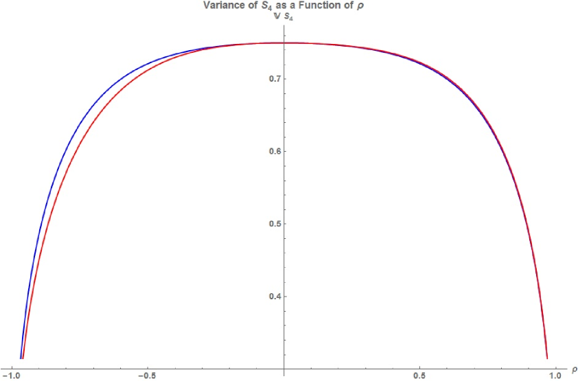
Figure 1: The red curve is an IIA-based model prediction of variance, while the blue curve is our theoretical expression for variance. The blue curve is symmetric with respect to the vertical axis; the red curve is not.

3 Appendix

With regard to $n=5$, David [18, 19] demonstrated how the inclusion-exclusion principle can be applied to compute $p_{11111}=q_{12345}$.  Twenty-eight of the thirty terms in her expansion:

$$q_{12345} =\tfrac{1}{2}\left(1-q_{1}-q_{2}-q_{3}-q_{4}-q_{5}+q_{12}+q_{13}+q_{14}+q_{15}+q_{23}+q_{24}+q_{25}+q_{34}+q_{35}+q_{45}\right.$$

$$\;\;\;\;\;\;\;-q_{123}-q_{124}-q_{125}-q_{134}-q_{135}-q_{145}-q_{234}-q_{235}-q_{245}-q_{345}$$

$$\left.\;\;\;\;\;\;\;+\,q_{1234}+q_{1235}+q_{1245}+q_{1345}+q_{2345}\right)$$

can be easily evaluated.  For example,

$$q_{1245}=\mathbb{P}\left\{X_{1}>0\text{, }X_{2}>0\text{, }X_{4}>0\text{ and }X_{5}>0\right\}$$

possesses a closed-form expression because

$$\operatorname{Cov}\left(\begin{array}[c]{c}X_{1}\\ X_{2}\\ X_{4}\\ X_{5}\end{array}\right)=\left(\begin{array}[c]{cccc}1&\rho&\rho^{3}&\rho^{4}\\ \rho&1&\rho^{2}&\rho^{3}\\ \rho^{3}&\rho^{2}&1&\rho\\ \rho^{4}&\rho^{3}&\rho&1\end{array}\right)$$

and this is of the form $R^{+}$ with $a=\rho$, $b=\rho^{2}$.  The orthant probability is

$$\frac{1}{16}+\frac{2\arcsin(\rho)+\arcsin\left(\rho^{2}\right)+2\arcsin\left(\rho^{3}\right)+\arcsin\left(\rho^{4}\right)}{8\pi}+\frac{\arcsin(\rho)^{2}+I(\rho,\rho^{4})}{4\pi^{2}}$$

which is $0.1337768212694702494423619...$ when $\rho=1/2$.

The two outlying terms:

$$\begin{array}[c]{ccc}\mathbb{P}\left\{X_{1}>0\text{, }X_{2}>0\text{, }X_{3}>0\text{ and }X_{5}>0\right\},&&\mathbb{P}\left\{X_{1}>0\text{, }X_{3}>0\text{, }X_{4}>0\text{ and }X_{5}>0\right\}\end{array}$$

are associated with matrices

$$\begin{array}[c]{ccc}\left(\begin{array}[c]{cccc}1&\rho&\rho^{2}&\rho^{4}\\ \rho&1&\rho&\rho^{3}\\ \rho^{2}&\rho&1&\rho^{2}\\ \rho^{4}&\rho^{3}&\rho^{2}&1\end{array}\right),&&\left(\begin{array}[c]{cccc}1&\rho^{2}&\rho^{3}&\rho^{4}\\ \rho^{2}&1&\rho&\rho^{2}\\ \rho^{3}&\rho&1&\rho\\ \rho^{4}&\rho^{2}&\rho&1\end{array}\right)\end{array}$$

of a type so far unseen.  The integral:

$$J(h,k,x)={\displaystyle\int\limits_{0}^{x}}\arcsin\left(\frac{\sqrt{1-h^{2}}\sqrt{1-k^{2}}\,t}{\sqrt{h^{2}-t^{2}}\sqrt{k^{2}-t^{2}}}\right)\frac{1}{\sqrt{1-t^{2}}}\,dt$$

resists symbolic attack if $h\neq k$, but is nevertheless accessible to very high-precision numerics.  The two orthant probabilities are both equal to

$$\frac{1}{16}+\frac{2\arcsin(\rho)+2\arcsin\left(\rho^{2}\right)+\arcsin\left(\rho^{3}\right)+\arcsin\left(\rho^{4}\right)}{8\pi}+\frac{\arcsin(\rho)\arcsin\left(\rho^{2}\right)+J(\rho,\rho^{2},\rho^{4})}{4\pi^{2}}$$

which is $0.1354451520661386999235683...$ when $\rho=1/2$.

We close with two comments.  First, our dilogarithm formula for $I(h,x)$ differs in appearance from Cheng’s formula [6] since he employed $\operatorname{Li}_{2}[r,\theta]$ to represent the real part of $\operatorname{Li}_{2}\left(r\cdot e^{i\theta}\right)$, whereas we use

$$\begin{array}[c]{ccc}\operatorname{Li}_{2}\left(z\right)+\operatorname{Li}_{2}\left(\overline{z}\right)=2\operatorname{Re}\left[\operatorname{Li}_{2}\left(z\right)\right]&&\text{for }z\in\mathbb{C}\setminus(1,\infty)\end{array}$$

to avoid this complication.  Finally, given $0<k<1$, in an artificial construct when

$$\begin{array}[c]{ccc}h=\dfrac{\sqrt{3}}{2},&&x=\sqrt{\dfrac{1-\sqrt{1-k^{2}}}{2}}\end{array}$$

the integral $J(h,k,x)$ can be found [8]:

$$\frac{\pi^{2}}{8}-\frac{\pi}{6}\arcsin\left(\ell\right)+\frac{1}{6}\arcsin(\ell)^{2}-\frac{\pi}{2}\arcsin\left(\sqrt{\frac{1-\ell}{2}}\right)-\frac{1}{3}\operatorname{Li}_{2}\left[-m^{2}\right]$$

$$-\frac{2}{3}\operatorname{Li}_{2}\left[(\ell+ik)m\right]-\frac{2}{3}\operatorname{Li}_{2}\left[(\ell-ik)m\right]+\frac{1}{3}\operatorname{Li}_{2}\left[(\ell+ik)m^{2}\right]+\frac{1}{3}\operatorname{Li}_{2}\left[(\ell-ik)m^{2}\right]$$

where

$$\begin{array}[c]{ccc}\ell=\sqrt{1-k^{2}},&&m=\dfrac{1+\ell-\sqrt{1+3\ell}\,\sqrt{1-\ell}}{2\ell}.\end{array}$$

This is a tantalizing hint that perhaps $J(\rho,\rho^{2},\rho^{4})$ is within grasp if $\rho=\sqrt{3}/2$.  Such a breakthrough will occur only if $x$ can be unlocked from its current fixed location and allowed to wander free.

4 Acknowledgements

Helpful correspondence with Andreas Dieckmann [20] and Tobias Ambjörnsson [17] is greatly appreciated.  Virtually all computations were performed within Mathematica.  The pmvnorm function, part of the mvtnorm package [21] within R, was useful for verification (impressive numerics: 12 digits of precision or better).

After the writing of this paper was completed, I learned of [22, 23], which utilize similar techniques in answering somewhat different questions.  More aspects of AR(1) are covered in [24, 25].

The cadence in much of Section 1 follows Emily Dickinson’s lines “Because I could not stop for Death – He kindly stopped for me”.  This paper is dedicated to the memory of my parents.

References

[1]S. S. Gupta, Probability integrals of multivariate normal
and multivariate , Annals Math. Statist. 34 (1963) 792–828;
MR0152068 [formulas (41) & (42)].
[2]S. S. Gupta, Bibliography on the multivariate normal
integrals and related topics, Annals Math. Statist. 34 (1963)
829–838; MR0152069.
[3]D. B. Owen, Orthant probabilities, Encyclopedia of
Statistical Sciences, v. 6, ed. S. Kotz, N. L. Johnson and C. B. Read, Wiley,
1985, pp. 521–523; MR0873585.
[4]Y. L. Tong, The Multivariate Normal Distribution,
Springer-Verlag, 1990, pp. 188-190; MR1029032.
[5]A. Genz and F. Bretz, Computation of Multivariate
Normal and Probabilities, Lect. Notes in Statist 195,
Springer-Verlag, 2009, pp. 11-12; MR2840595.
[6]M. C. Cheng, The orthant probabilites of four Gaussian
variates, Annals Math. Statist. 40 (1969) 152–161; MR0235596 [error
in formula (2.21) requires correction: product should be ].
[7]M. C. Cheng, Output autocorrelation functions of smooth and
hard limiters, Internat. J. Control 7 (1968) 223–240.
[8]M. C. Cheng, On a class of integrals expressible in terms of
, and , Nanta Math. 4 (1970) 113–116; MR0304709.
[9]Z. Ni and B. Kedem, On normal orthant probabilities,
Chinese J. Appl. Probab. Statist., v. 15 (1999) n. 3, 262–275; MR1771106.
[10]S. O. Rice, Mathematical analysis of random noise,
Bell System Tech. J. 23 (1944) 282–332; 24 (1945) 46–156; also in
Selected Papers on Noise and Stochastic Processes, ed. N. Wax, Dover,
1954, pp. 133–294; MR0010932 and MR0011918.
[11]S. R. Finch, Zero crossings, Mathematical Constants
II, Cambridge Univ. Press, 2019, pp. 479–485; MR2003519.
[12]B. Kedem, Time Series Analysis by Higher Order
Crossings, IEEE Press, 1994, pp. 115–143; MR1261636.
[13]J. T. Barnett, Zero-crossings of random processes with
application to estimation and detection, Nonuniform Sampling: Theory
and Practice, ed. F. Marvasti, Kluwer/Plenum, 2001, pp. 393–435; MR1875683.
[14]A. J. F. Siegert, On the first passage time probability
problem, Phys. Rev. 81 (1951) 617–623; MR0054192.
[15]J. A. McFadden, The axis-crossing intervals of random
functions. II, IEEE Trans. Inform. Theory (1958) 14–24; MR0098437.
[16]M. Nyberg, T. Ambjörnsson and L. Lizana, A simple method
to calculate first-passage time densities with arbitrary initial conditions,
New J. Phys. 18 (2016) 063019.
[17]M. Nyberg, L. Lizana and T. Ambjörnsson, Zero-crossing
statistics for non-Markovian time series, Phys. Rev. E 97 (2018)
032114; arXiv:1711.02926 [beware of typo in preprint version: plus sign should
be minus sign in formulas (3) & (25)].
[18]F. N. David, A note on the evaluation of the multivariate
normal integral, Biometrika 40 (1953) 458–459; MR0058314.
[19]T. Guillaume, Computation of the quadrivariate and
pentavariate normal cumulative distribution functions, Comm. Statist.
Simulat. Comput. 47 (2018) 839–851; MR3810596.
[20]A. Dieckmann, Table of Indefinite Integrals,
http://www-elsa.physik.uni-bonn.de/~dieckman/IntegralsIndefinite/IndefInt.html.
[21]X. Mi, T. Miwa and T. Hothorn, New numerical algorithm for
multivariate normal probabilities in package mvtnorm, The R Journal 1
(2009) pp. 37–39; http://journal.r-project.org/archive/2009-1/.
[22]S. M. Stigler, Estimating serial correlation by visual
inspection of diagnostic plots, Amer. Statist. 40 (1986) 111–116; MR0841577.
[23]S. Ku and E. Seneta, The number of peaks in a stationary
sample and orthant probabilities, J. Time Series Analysis 15 (1994)
385–403; MR1292616.
[24]S. Finch, Moments of maximum: Segment of AR(1), arXiv:1908.04179.
[25]S. Finch, Another look at AR(1), arXiv:0710.5419.