Fundamental tones of clamped plates in nonpositively curved spaces

Abstract.

We study Lord Rayleigh’s problem for clamped plates on an arbitrary $n$-dimensional $(n\geq 2)$ Cartan-Hadamard manifold $(M,g)$ with sectional curvature $\textbf{K}\leq-\kappa^{2}$ for some $\kappa\geq 0.$ We first prove a McKean-type spectral gap estimate, i.e. the fundamental tone of any domain in $(M,g)$ is universally bounded from below by $\frac{(n-1)^{4}}{16}\kappa^{4}$ whenever the $\kappa$-Cartan-Hadamard conjecture holds on $(M,g)$, e.g. in 2- and 3-dimensions due to Bol (1941) and Kleiner (1992), respectively. In 2- and 3-dimensions we prove sharp isoperimetric inequalities for sufficiently small clamped plates, i.e. the fundamental tone of any domain in $(M,g)$ of volume $v>0$ is not less than the corresponding fundamental tone of a geodesic ball of the same volume $v$ in the space of constant curvature $-\kappa^{2}$ provided that $v\leq c_{n}/\kappa^{n}$ with $c_{2}\approx 21.031$ and $c_{3}\approx 1.721$, respectively. In particular, Rayleigh’s problem in Euclidean spaces resolved by Nadirashvili (1992) and Ashbaugh and Benguria (1995) appears as a limiting case in our setting (i.e. $\textbf{K}\equiv\kappa=0$). Sharp asymptotic estimates of the fundamental tone of small and large geodesic balls of low-dimensional hyperbolic spaces are also given. The sharpness of our results requires the validity of the $\kappa$-Cartan-Hadamard conjecture (i.e. sharp isoperimetric inequality on $(M,g)$) and peculiar properties of the Gaussian hypergeometric function, both valid only in dimensions 2 and 3; nevertheless, some nonoptimal estimates of the fundamental tone of arbitrary clamped plates are also provided in high-dimensions. As an application, by using the sharp isoperimetric inequality for small clamped hyperbolic discs, we give necessarily and sufficient conditions for the existence of a nontrivial solution to an elliptic PDE involving the biharmonic Laplace-Beltrami operator.

Dedicated to Professor Biagio Ricceri on the occasion of his 65th anniversary.

1. Introduction and Main Results

Let $\Omega\subset\mathbb{R}^{n}$ be a bounded domain $(n\geq 2)$, and consider the eigenvalue problem

$$\left\{\begin{array}[]{lll}\Delta^{2}u=\Gamma u&\mbox{in}&\Omega,\\ u=|\nabla u|=0&\mbox{on}&\partial\Omega,\end{array}\right.$$ (1.1)

associated with the vibration of a clamped plate. The lowest/principal eigenvalue for (1.1) – the fundamental tone of the clamped plate – can be characterized in a variational way by

$$\Gamma_{0}(\Omega)=\inf_{u\in W_{0}^{2,2}(\Omega)\setminus\{0\}}\frac{\displaystyle\int_{\Omega}(\Delta u)^{2}{\rm d}x}{\displaystyle\int_{\Omega}u^{2}{\rm d}x}.$$ (1.2)

The minimizer of (1.2) in the plane describes the vibration of a homogeneous thin plate $\Omega\subset\mathbb{R}^{2}$ whose boundary is clamped, while the frequency of vibration of the plate $\Omega$ is proportional to $\Gamma_{0}(\Omega)^{\frac{1}{2}}.$ The famous conjecture of Lord Rayleigh [36, p.382] – formulated initially for planar domains in 1894 – states that

$$\Gamma_{0}(\Omega)\geq\Gamma_{0}(\Omega^{\star})=\mathfrak{h}^{4}_{\nu}\left(\frac{\omega_{n}}{|\Omega|}\right)^{4/n},$$ (1.3)

where $\Omega^{\star}\subset\mathbb{R}^{n}$ is a ball with the same measure as $\Omega$, with equality if and only if $\Omega$ is a ball. Hereafter, $\nu=\frac{n}{2}-1$, $\omega_{n}=\pi^{n/2}/\Gamma(1+n/2)$ is the volume of the unit Euclidean ball, while $\mathfrak{h}_{\nu}$ is the first positive critical point of $\frac{J_{\nu}}{I_{\nu}}$, where $J_{\nu}$ and $I_{\nu}$ stand for the Bessel and modified Bessel functions of first kind, respectively.

Assuming that the eigenfunction corresponding to $\Gamma_{0}(\Omega)$ is sign-preserving over a simply connected domain $\Omega\subset\mathbb{R}^{2}$, Szegő [38] proved (1.3) in the early fifties. As one can deduce from his paper’s text, his belief on the constant-sign first eigenfunction corresponding to $\Gamma_{0}(\Omega)$ has been based on the second-order membrane problem (called as the Faber-Krahn problem). It turned out shortly that his expectation perishes due to the construction of Duffin [19] on strip-like domains and Coffman, Duffin and Shaffer [16] on ring-shaped clamped plate, localizing nodal lines of vibrating plates. While the membrane problem involves only the Laplacian, the clamped plate problem requires the presence of the fourth order bilaplacian operator; as we know nowadays, fourth order equations are lacking general maximum/comparison principles which is unrevealed in Szegő’s pioneering approach. In fact, stimulated by the papers [19] and [16], several scenarios are described for nodal domains of clamped plates, see e.g. Bauer and Reiss [3], Coffman [15], Grunau and Robert [21], from which the main edification is that eigenfunctions corresponding to (1.2) may change their sign.

In order to handle the presence of possible nodal domains, Talenti [40] developed a Schwarz-type rearrangement method on domains where the first eigenfunction corresponding to (1.2) has both positive and negative parts. In this way, a decomposition of (1.2) into a two-ball minimization problem arises which provided a nonoptimal estimate in (1.3); in fact, instead of (1.3), Talenti proved that $\Gamma_{0}(\Omega)\geq d_{n}\Gamma_{0}(\Omega^{\star})$ where the dimension-depending constant $d_{n}$ has the properties $\frac{1}{2}\leq d_{n}<1$ for every $n\geq 2$ and $\displaystyle\lim_{n\to\infty}d_{n}=\frac{1}{2}.$

By a careful improvement of Talenti’s two-ball minimization argument, Rayleigh’s conjecture has been proved in its full generality for $n=2$ by Nadirashvili [31, 32]. Further modifications of some arguments from the papers [32] and [40] allowed to Ashbaugh and Benguria [1] to prove Rayleigh’s conjecture for $n=3$ (and $n=2$) by exploring fine properties of Bessel functions. Roughly speaking, for $n\in\{2,3\}$, the two-ball minimization problem reduces to only one ball (the other ball disappearing), while in higher dimensions the ’optimal’ situation appears for two identical balls which provides a nonoptimal estimate for $\Gamma_{0}(\Omega)$. Although asymptotically sharp estimates are provided by Ashbaugh and Laugesen [2] for $\Gamma_{0}(\Omega)$ in high-dimensions, i.e. $\displaystyle\Gamma_{0}(\Omega)\geq D_{n}\Gamma_{0}(\Omega^{\star})$ where $0.89<D_{n}<1$ for every $n\geq 4$ with $\displaystyle\lim_{n\to\infty}D_{n}=1$, the conjecture is still open for $n\geq 4$. Very recently, Chasman and Langford [6, 7] provided certain Ashbaugh-Laugesen-type results in Euclidean spaces endowed with a log-convex/Gaussian density, by proving that $\Gamma_{w}(\Omega)\geq\tilde{C}\Gamma_{w}(\Omega^{\star})$, where the constant $\tilde{C}\in(0,1)$ depends on the volume of $\Omega$ and dimension $n\geq 2$, while $\Gamma_{w}(\Omega)$ and $\Gamma_{w}(\Omega^{\star})$ denote the fundamental tones of the clamped plate with respect to the corresponding density function $w$.

Interest in the clamped plate problem on curved spaces was also increased in recent years. One of the most central problems is to establish Payne-Pólya-Weinberger-Yang-type inequalities for the eigenvalues of the problem

$$\left\{\begin{array}[]{lll}\Delta_{g}^{2}u=\Gamma u&\mbox{in}&\Omega,\\ u=\frac{\partial u}{\partial\textbf{n}}=0&\mbox{on}&\partial\Omega,\end{array}\right.$$ (1.4)

where $\Omega$ is a bounded domain in an $n$-dimensional Riemannian manifold $(M,g)$, $\Delta_{g}^{2}$ stands for the biharmonic Laplace-Beltrami operator on $(M,g)$ and $\frac{\partial}{\partial\textbf{n}}$ is the outward normal derivative on $\partial\Omega$, respectively; see e.g. Chen, Zheng and Lu [9], Cheng, Ichikawa and Mametsuka [10], Cheng and Yang [11, 12, 13], Wang and Xia [42]. Instead of (1.2), one naturally considers the fundamental tone of $\Omega\subset M$ by

$$\Gamma_{g}(\Omega):=\Gamma_{g,n}(\Omega)=\inf_{u\in W_{0}^{2,2}(\Omega)\setminus\{0\}}\frac{\displaystyle\int_{\Omega}(\Delta_{g}u)^{2}{\rm d}v_{g}}{\displaystyle\int_{\Omega}u^{2}{\rm d}v_{g}},$$ (1.5)

where ${\rm d}v_{g}$ denotes the canonical measure on $(M,g)$, and $W_{0}^{2,2}(\Omega)$ is the usual Sobolev space on $(M,g)$, see Hebey [22]; in fact, it turns out that $\Gamma_{g}(\Omega)$ is the first eigenvalue to (1.4). Due to the Bochner-Lichnerowicz-Weitzenböck formula, the Sobolev space $H_{0}^{2}(\Omega)=W_{0}^{2,2}(\Omega)$ is a proper choice for (1.4), see Proposition 3.1 for details.

To the best of our knowledge, no results – comparable to (1.3) – are available in the literature concerning Lord Rayleigh’s problem for clamped plates on curved structures. Accordingly, the main purpose of the present paper is to identify those geometric and analytic properties which reside in Lord Rayleigh’s problem for clamped plates on nonpositively curved spaces. To develop our results, the geometric context is provided by an $n$-dimensional $(n\geq 2)$ Cartan-Hadamard manifold $(M,g)$ (i.e. simply connected, complete Riemannian manifold with nonpositive sectional curvature). Having this framework, we recall McKean’s spectral gap estimate for membranes which is closely related to (1.5); namely, in an $n$-dimensional Cartan-Hadamard manifold $(M,g)$ with sectional curvature ${{\rm\bf K}}\leq-\kappa^{2}$ for some $\kappa>0,$ the principal frequency of any membrane $\Omega\subset M$ can be estimated as

$$\gamma_{g}(\Omega):=\inf_{u\in W_{0}^{1,2}(\Omega)\setminus\{0\}}\frac{\displaystyle\int_{\Omega}|\nabla_{g}u|^{2}{\rm d}v_{g}}{\displaystyle\int_{\Omega}u^{2}{\rm d}v_{g}}\geq\frac{(n-1)^{2}}{4}\kappa^{2};$$ (1.6)

in addition, (1.6) is sharp on the $n$-dimensional hyperbolic space $(\mathbb{H}_{-\kappa^{2}}^{n},g_{\kappa})$ of constant curvature $-\kappa^{2}$ in the sense that $\gamma_{g_{\kappa}}(\Omega)\to\frac{(n-1)^{2}}{4}\kappa^{2}$ whenever $\Omega$ tends to $\mathbb{H}_{-\kappa^{2}}^{n}$, see McKean [30].

Before to state our results, we fix some notations. If $\kappa\geq 0$, let $N^{n}_{\kappa}$ be the $n$-dimensional space-form with constant sectional curvature $-\kappa^{2}$, i.e. $N^{n}_{\kappa}$ is either the hyperbolic space $\mathbb{H}_{-\kappa^{2}}^{n}$ when $k>0$, or the Euclidean space $\mathbb{R}^{n}$ when $\kappa=0.$ Let $B_{\kappa}(L)$ be the geodesic ball of radius $L>0$ in $N^{n}_{\kappa}$ and if $\Omega\subset N^{n}_{\kappa}$, we denote by $\Gamma_{\kappa}(\Omega)$ the corresponding value from (1.5). By convention, we consider $1/0=+\infty$ and as usual, $V_{g}(S)$ denotes the Riemannian volume of $S\subset M$.

Our first result provides a fourth order counterpart of McKean’s spectral gap estimate, which requires the validity of the $\kappa$-Cartan-Hadamard conjecture on $(M,g)$; the latter is nothing but the sharp isoperimetric inequality on $(M,g)$, which is valid e.g. on hyperbolic spaces of any dimension as well as on generic 2- and 3-dimensional Cartan-Hadamard manifolds with sectional curvature ${{\rm\bf K}}\leq-\kappa^{2}$ for some $\kappa\geq 0,$ see §2.2.

Theorem 1.1.

Let $(M,g)$ be an $n$-dimensional Cartan-Hadamard manifold with sectional curvature ${{\rm\bf K}}\leq-\kappa^{2}$ for some $\kappa\geq 0,$ which verifies the $\kappa$-Cartan-Hadamard conjecture. If $\Omega\subset M$ is a bounded domain with smooth boundary then

$$\Gamma_{g}(\Omega)\geq\frac{(n-1)^{4}}{16}\kappa^{4}.$$ (1.7)

Moreover, for $n\in\{2,3\}$, relation (1.7) is sharp in the sense that

$$\Gamma_{\kappa}(N^{n}_{\kappa}):=\lim_{L\to\infty}\Gamma_{\kappa}(B_{\kappa}(L))=\frac{(n-1)^{4}}{16}\kappa^{4}.$$ (1.8)

Clearly, Theorem 1.1 is relevant only for $\kappa>0$ (as (1.7) and (1.8) trivially hold for $\kappa=0$). Moreover, if $n\in\{2,3\}$ and $\kappa>0$, and $\Gamma_{\kappa}^{l}(\Omega)$ denotes the $l^{\rm th}$ eigenvalue of (1.4) on $\Omega\subset\mathbb{H}_{-\kappa^{2}}^{n}$, then making use of (1.8) and a Payne-Pólya-Weinberger-Yang-type universal inequality on $\mathbb{H}_{-\kappa^{2}}^{n}$, it turns out that

$$\Gamma_{\kappa}^{l}(\mathbb{H}_{-\kappa^{2}}^{n}):=\lim_{L\to\infty}\Gamma_{\kappa}^{l}(B_{\kappa}(L))=\frac{(n-1)^{4}}{16}\kappa^{4}\ \ {\rm for\ all}\ \ l\in\mathbb{N}.$$ (1.9)

In particular, (1.9) confirms a claim of Cheng and Yang [12, Theorem 1.4] for $n\in\{2,3\}$, where the authors assumed (1.8) itself in order to derive (1.9). In fact, one can expect the validity of (1.9) for any $n\geq 2$ but some technical difficulties prevent the proof in high-dimensions; for details, see §5.3.

Actually, Theorem 1.1 is just a byproduct of a general argument needed to prove the main result of our paper (for its statement, we recall that $\mathfrak{h}_{\nu}$ is the first positive critical point of $\frac{J_{\nu}}{I_{\nu}}$ and $\nu=\frac{n}{2}-1$):

Theorem 1.2.

Let $n\in\{2,3\}$ and $(M,g)$ be an $n$-dimensional Cartan-Hadamard manifold with sectional curvature ${{\rm\bf K}}\leq-\kappa^{2}$ for some $\kappa\geq 0,$ $\Omega\subset M$ be a bounded domain with smooth boundary and volume $V_{g}(\Omega)\leq\frac{c_{n}}{\kappa^{n}}$ with $c_{2}\approx 21.031$ and $c_{3}\approx 1.721.$ If $\Omega^{\star}\subset N^{n}_{\kappa}$ is a geodesic ball verifying $V_{g}(\Omega)=V_{\kappa}(\Omega^{\star})$ then

$$\Gamma_{g}(\Omega)\geq\Gamma_{\kappa}(\Omega^{\star}),$$ (1.10)

with equality in (1.10) if and only if $\Omega$ is isometric to $\Omega^{\star}.$ Moreover,

$$\Gamma_{\kappa}(B_{\kappa}(L))\sim\left({\frac{(n-1)^{2}}{4}{\kappa^{2}}+\frac{\mathfrak{h}_{\nu}^{2}}{L^{2}}}\right)^{2}\ \ \mbox{as}\ \ L\to 0.$$ (1.11)

Some comments are in order.

The proof of Theorems 1.1 and 1.2 is based on a decomposition argument similar to the one carried out by Talenti [40] and Ashbaugh and Benguria [1] in the Euclidean framework. In fact, we transpose the original variational problem from generic nonpositively curved spaces to the space-form $N_{\kappa}^{n}$ by assuming the validity of the $\kappa$-Cartan-Hadamard conjecture on $(M,g)$. By a fourth order ODE it turns out that $\Gamma_{\kappa}(\Omega^{\star})$ is the smallest positive solution to the cross-product of suitable Gaussian hypergeometric functions (resp., Bessel functions) whenever $\kappa>0$ (resp., $\kappa=0$). The aforementioned decomposition argument combined with certain oscillatory and asymptotic properties of the hypergeometric function provides the proof of Theorem 1.1.

The dimensionality restriction $n\in\{2,3\}$ in Theorem 1.2 (and relation (1.8)) is needed not only for the validity of the $\kappa$-Cartan-Hadamard conjecture but also for some peculiar properties of the Gaussian hypergeometric function; similar phenomenon has been pointed out also by Ashbaugh and Benguria [1] in the Euclidean setting for Bessel functions. In addition, the arguments in Theorem 1.2 work only for sets with sufficiently small measure; unlike the usual Lebesgue measure in $\mathbb{R}^{n}$ (where the scaling $\Gamma_{0}(B_{0}(L))=L^{-4}\Gamma_{0}(B_{0}(1))$ holds for every $L>0$), the inhomogeneity of the canonical measure on hyperbolic spaces requires the aforementioned volume-restriction. The intuitive feeling we get that eigenfunctions corresponding to $\Gamma_{g}(\Omega)$ on a large domain $\Omega\subset M$ with strictly negative curvature may have large nodal domains whose symmetric rearrangements in $\mathbb{H}_{-\kappa^{2}}^{n}$ produce large geodesic balls and their ’joined’ fundamental tone can be definitely lower than the expected $\Gamma_{\kappa}(\Omega^{\star})$. In fact, our arguments show that Theorem 1.2 cannot be improved even if we restrict the setting to the model space-form $\mathbb{H}_{-\kappa^{2}}^{n}$. It remains an open question whether or not (1.10) remains valid for arbitrarily large domains in any dimension $n\geq 4$; we notice however that some nonoptimal estimates of $\Gamma_{g}(\Omega)$ are also provided for any domain in high-dimensions (see §5.4). The asymptotic property (1.11) for $\kappa>0$ follows by an elegant asymptotic connection between hypergeometric and Bessel functions, which is crucial in the proof of (1.10) and its accuracy is shown in Table 1 (see §5.2) for some values of $L\ll 1$. Clearly, (1.11) is trivial for $\kappa=0$ since $\Gamma_{0}(B_{0}(L))=\mathfrak{h}_{\nu}^{4}/L^{4}$ for every $L>0$.

A natural question arises concerning the sharp estimate of the fundamental tone on complete $n$-dimensional Riemannian manifolds with Ricci curvature Ric${}_{(M,g)}\geq k(n-1)$ for some $k\geq 0$. Some arguments based on the spherical Laplacian show that Bessel functions (when $k=0$) and Gaussian hypergeometric functions (when $k>0$) will play again crucial roles. Since the parameter range of the aforementioned special functions in the nonnegatively curved case is different from the present setting, further technicalities appear which require a deep analysis. Accordingly, we intend to come back to this problem in a forthcoming paper.

As an application of Theorem 1.2, we consider the elliptic problem

$$\ \left\{\begin{array}[]{lll}\Delta_{\kappa}^{2}u-\mu\Delta_{\kappa}u+\gamma u=|u|^{p-2}u&{\rm in}&B_{\kappa}(L),\\ u\geq 0,\ u\in W_{0}^{2,2}(B_{\kappa}(L)),\end{array}\right.$$

where $B_{\kappa}(L)\subset\mathbb{H}_{-\kappa^{2}}^{2}$ is a hyperbolic disc and the range of parameters $\mu,\gamma,p,\kappa$ and $L$ is specified below. By using variational arguments, one can prove the following result.

Theorem 1.3.

Let $\mu\geq 0$, $\gamma\in\mathbb{R}$, $p>2$, $\kappa>0$ and $0<L<\frac{2.1492}{\kappa}.$ The following statements hold$:$

• if $\mu=0$ and problem $({\mathcal{P}})$ admits a nonzero solution then $\gamma>-\Gamma_{\kappa}(B_{k}(L));$

• if $\mu>0$ and $\gamma>-\Gamma_{\kappa}(B_{k}(L))$ then problem $({\mathcal{P}})$ admits a nonzero solution.

The paper is organized as follows. In Section 2 we recall/prove those notions/results which are indispensable in our study (space-forms, $\kappa$-Cartan-Hadamard conjecture, oscillatory properties of specific Gaussian hypergeometric functions). In Section 3 we develop an Ashbaugh-Benguria-Talenti-type decomposition from curved spaces to space-forms. In Sections 4 and 5 we provide a McKean-type spectral gap estimate (proof of Theorem 1.1) and comparison principles (proof of Theorem 1.2) for fundamental tones, respectively. In Section 6 we prove Theorem 1.3.

2. Preliminaries

2.1. Space-forms.

Let $\kappa\geq 0$ and $N^{n}_{\kappa}$ be the $n$-dimensional space-form with constant sectional curvature $-\kappa^{2}$. When $\kappa=0$, $N_{\kappa}^{n}=\mathbb{R}^{n}$ is the usual Euclidean space, while for $\kappa>0$, $N^{n}_{\kappa}$ is the $n$-dimensional hyperbolic space represented by the Poincaré ball model $N_{\kappa}^{n}=\mathbb{H}^{n}_{-\kappa^{2}}=\{x\in\mathbb{R}^{n}:|x|<1\}$ endowed with the Riemannian metric

$$g_{\kappa}(x)=(g_{ij}(x))_{i,j={1,...,n}}=p^{2}_{\kappa}(x)\delta_{ij},$$

where $p_{\kappa}(x)=\frac{2}{\kappa(1-|x|^{2})}.$ $(\mathbb{H}^{n}_{-\kappa^{2}},g_{\kappa})$ is a Cartan-Hadamard manifold with constant sectional curvature $-\kappa^{2}$. If $\nabla$ and div denote the Euclidean gradient and divergence operator in $\mathbb{R}^{n},$ the canonical volume form, gradient and Laplacian operator on $N^{n}_{\kappa}$ are

$${\text{d}}v_{\kappa}(x)=\left\{\begin{array}[]{lll}{\text{d}}x&\mbox{if}&\kappa=0,\\ p^{n}_{\kappa}(x){\text{d}}x&\mbox{if}&\kappa>0,\end{array}\right.\ \ \nabla_{\kappa}u=\left\{\begin{array}[]{lll}\nabla u&\mbox{if}&\kappa=0,\\ \frac{\nabla u}{p_{\kappa}^{2}}&\mbox{if}&\kappa>0,\end{array}\right.$$

and

$$\Delta_{\kappa}u=\left\{\begin{array}[]{lll}\Delta u&\mbox{if}&\kappa=0,\\ p_{\kappa}^{-n}{\rm div}(p_{\kappa}^{n-2}\nabla u)&\mbox{if}&\kappa>0,\end{array}\right.$$

respectively. The distance function on $N^{n}_{\kappa}$ is denoted by $d_{\kappa}$; the distance between the origin and $x\in N^{n}_{\kappa}$ is given by

$$d_{\kappa}(x):=d_{\kappa}(0,x)=\left\{\begin{array}[]{lll}|x|&\mbox{if}&\kappa=0,\\ \frac{1}{\kappa}\ln\left(\frac{1+|x|}{1-|x|}\right)&\mbox{if}&\kappa>0.\end{array}\right.$$

The volume of the geodesic ball $B_{\kappa}(r)=\{x\in N^{n}_{\kappa}:d_{\kappa}(x)<r\}$ is

$$V_{\kappa}(r):=V_{\kappa}(B_{\kappa}(r))=n\omega_{n}\int_{0}^{r}{\mathbf{s}}_{\kappa}(\rho)^{n-1}{\rm d}\rho,$$ (2.1)

where

$${\mathbf{s}}_{\kappa}(\rho)=\left\{\begin{array}[]{lll}\rho&\mbox{if}&\kappa=0,\\ \frac{\sinh(\kappa\rho)}{\kappa}&\mbox{if}&\kappa>0.\end{array}\right.$$

A simple change of variables gives the following useful transformation.

Proposition 2.1.

Let $\kappa\geq 0.$ For every integrable function $g:[0,L]\to\mathbb{R}$ with $L\geq 0$ one has

$$\int_{0}^{L}g(s){\rm d}s=\int_{B_{\kappa}({r_{L}})}g(V_{\kappa}(d_{\kappa}(x))){\rm d}v_{\kappa}(x),$$

where $r_{L}\geq 0$ is the unique real number verifying $V_{k}({r_{L}})=L.$

2.2. $\kappa$-Cartan-Hadamard conjecture

Let $(M,g)$ be an $n$-dimensional Cartan-Hadamard manifold with sectional curvature bounded above by $-\kappa^{2}$ for some $\kappa\geq 0$. The $\kappa$-Cartan-Hadamard conjecture on $(M,g)$ (called also as the generalized Cartan-Hadamard conjecture) states that the $\kappa$-sharp isoperimetric inequality holds on $(M,g)$, i.e. for every open bounded $\Omega\subset M$ one has

$$A_{g}(\partial\Omega)\geq A_{\kappa}(\partial B_{\kappa}(r)),$$ (2.2)

whenever $V_{g}(\Omega)=V_{\kappa}(r)$; moreover, equality holds in (2.2) if and only if $\Omega$ is isometric to $B_{\kappa}(r)$. Hereafter, $A_{g}$ and $A_{\kappa}$ stand for the area on $(M,g)$ and $N_{\kappa}^{n}$, respectively.

The $\kappa$-Cartan-Hadamard conjecture holds for every $\kappa\geq 0$ on space-forms with constant sectional curvature $-\kappa^{2}$ (of any dimension), see Dinghas [18], and on Cartan-Hadamard manifolds with sectional curvature bounded above by $-\kappa^{2}$ of dimension $2$, see Bol [5], and of dimension $3$, see Kleiner [26]. In addition, a very recent result of Ghomi and Spruck [20] states that the $0$-Cartan-Hadamard conjecture holds in any dimension; in dimension 4, the validity of the $0$-Cartan-Hadamard conjecture is due to Croke [14]. In higher dimensions and for $\kappa>0,$ the conjecture is still open; for a detailed discussion, see Kloeckner and Kuperberg [28].

2.3. Gaussian hypergeometric function

For $a,b,c\in\mathbb{C}$ ($c\neq 0,-1,-2,...$) the Gaussian hypergeometric function is defined by

$${\bf F}(a,b;c;z)={{}_{2}F}_{1}(a,b;c;z)=\sum_{k\geq 0}\frac{(a)_{k}(b)_{k}}{(c)_{k}}\frac{z^{k}}{k!}$$ (2.3)

on the disc $|z|<1$ and extended by analytic continuation elsewhere, where $(a)_{k}=\frac{\Gamma(a+k)}{\Gamma(a)}$ denotes the Pochhammer symbol. The corresponding differential equation to $z\mapsto{\bf F}(a,b;c;z)$ is

$$z(1-z)w^{\prime\prime}(z)+(c-(a+b+1)z)w^{\prime}(z)-abw(z)=0.$$ (2.4)

We also recall the differentiation formula

$$\frac{\rm d}{{\rm d}z}{\bf F}(a,b;c;z)=\frac{ab}{c}{\bf F}(a+1,b+1;c+1;z).$$ (2.5)

Let $n\geq 2$ be an integer, $K>0$ be fixed, and consider the function

$$w^{K}_{\pm}(t)={\bf F}\left(\frac{1-\sqrt{(n-1)^{2}\pm 4\sqrt{K}}}{2},\frac{1+\sqrt{(n-1)^{2}\pm 4\sqrt{K}}}{2};\frac{n}{2};-t\right),\ \ t>0.$$

The following result will be indispensable in our study.

Proposition 2.2.

Let $K>0$ be fixed. The following properties hold$:$

• $w^{K}_{+}(t)>0$ for every $t\geq 0;$

• if $K\leq\frac{{(n-1)^{4}}}{16}$, then $w^{K}_{+}(t)\geq w^{K}_{-}(t)>0$ for every $t\geq 0;$

• $w^{K}_{-}$ is oscillatory on $(0,\infty)$ if and only if $K>\frac{{(n-1)^{4}}}{16}$.

Proof. For simplicity of notation, let $a_{\pm}=\frac{1-\sqrt{(n-1)^{2}\pm 4\sqrt{K}}}{2}$ and $b_{\pm}=\frac{1+\sqrt{(n-1)^{2}\pm 4\sqrt{K}}}{2}$.

(i) The connection formula (15.10.11) of Olver et al. [33] implies that

$$w^{K}_{+}(t)=(1+t)^{-b_{+}}{\bf F}\left(\frac{n}{2}-a_{+},b_{+};\frac{n}{2};\frac{t}{1+t}\right),\ t\geq 0.$$

Due to $\frac{n}{2}-a_{+}>0$, $b_{+}>0$ and (2.3), we have that $w^{K}_{+}(t)>0$ for every $t\geq 0.$

(ii) Fix $0<K\leq\frac{{(n-1)^{4}}}{16}$. First, since $\frac{n}{2}-a_{-}>0$ and $b_{-}>0$, the connection formula (15.10.11) of [33] together with (2.3) implies again that

$$w^{K}_{-}(t)=(1+t)^{-b_{-}}{\bf F}\left(\frac{n}{2}-a_{-},b_{-};\frac{n}{2};\frac{t}{1+t}\right)>0,\ t>0.$$

By virtue of (2.4), an elementary transformation shows that $w_{\pm}:=w^{K}_{\pm}$ verifies the ordinary differential equation

$$t(t+1)w_{\pm}^{\prime\prime}(t)+\left(2t+\frac{n}{2}\right)w_{\pm}^{\prime}(t)+\frac{1-(n-1)^{2}\mp 4\sqrt{K}}{4}w_{\pm}(t)=0,\ \ t>0.$$ (2.6)

It turns out that (2.6) is equivalent to

$$\left(p(t)w_{\pm}^{\prime}(t)\right)^{\prime}+q_{\pm}(t)w_{\pm}(t)=0,\ \ t>0,$$ (2.7)

where $p(t)=t^{\frac{n}{2}}(1+t)^{2-\frac{n}{2}}$, $q_{\pm}(t)=\tilde{K}_{\pm}t^{\frac{n}{2}-1}(1+t)^{1-\frac{n}{2}}$ and $\tilde{K}_{\pm}=\frac{1-(n-1)^{2}\mp 4\sqrt{K}}{4}$. For any $\tau>0$, relation (2.7) and a Sturm-type argument gives that

$$0 = \int_{0}^{\tau}\left[w_{-}\left(\left(pw_{+}^{\prime}\right)^{\prime}+q_{+}w_{+}\right)-w_{+}\left(\left(pw_{-}^{\prime}\right)^{\prime}+q_{-}w_{-}\right)\right]$$

$$= \int_{0}^{\tau}(q_{+}-q_{-})w_{-}w_{+}+\left[p\left(w_{-}w_{+}^{\prime}-w_{+}w_{-}^{\prime}\right)\right]\big{|}_{0}^{\tau}.$$

Since $q_{+}<q_{-}$, $p(0)=0$, and $w_{\pm}>0$, we necessarily have that $w_{-}w_{+}^{\prime}-w_{+}w_{-}^{\prime}\geq 0$ on $(0,\infty)$. In particular, $\frac{w_{+}}{w_{-}}$ is non-decreasing on $(0,\infty)$ and since $w_{+}(0)=w_{-}(0)=1$, we have that $w_{+}\geq w_{-}$ on $[0,\infty)$.

(iii) By (ii) we have $w^{K}_{-}(t)>0$ for every $t>0$ whenever $0<K\leq\frac{{(n-1)^{4}}}{16}$, i.e. $w^{K}_{-}$ is not oscillatory on $(0,\infty)$ for numbers $K$ belonging to this range.

Assume now that $K>\frac{{(n-1)^{4}}}{16}$. Since $\displaystyle\int_{\alpha}^{\infty}\frac{1}{p(t)}{\rm d}t<\infty$ for every $\alpha>0$, one can apply the result of Sugie, Kita and Yamaoka [39, Theorem 3.1] (see also Hille [23]), which states that if

$$p(t)q_{-}(t)\left(\displaystyle\int_{t}^{\infty}\frac{1}{p(\tau)}{\rm d}\tau\right)^{2}\geq\frac{1}{4}\ \ {\rm for}\ \ t\gg 1,$$ (2.8)

then the function $w^{K}_{-}$ in (2.7) is oscillatory. Due to the fact that

$$p(t)q_{-}(t)\left(\displaystyle\int_{t}^{\infty}\frac{1}{p(\tau)}{\rm d}\tau\right)^{2}\sim\tilde{K}_{-}\ \ \ {\rm as}\ \ t\to\infty,$$

and $\tilde{K}_{-}=\frac{1-(n-1)^{2}+4\sqrt{K}}{4}>\frac{1}{4}$, inequality (2.8) trivially holds, which concludes the proof. $\square$

Remark 2.1.

Dmitrii Karp kindly pointed out that for every $\beta\geq\frac{1}{2}$ and $t>0$, the function $x\mapsto{\bf F}(\frac{1}{2}-x,\frac{1}{2}+x;\beta;-t)$ is strictly increasing on $[0,\infty)$ from which Proposition 2.2/(ii) follows; his proof is based on fine properties of the hypergeometric functions ${}_{2}F_{1}$ and ${}_{3}F_{2}$, cf. Karp [24].

3. Ashbaugh-Benguria-Talenti-type decomposition: from curved spaces to space-forms

Without saying explicitly throughout this section, we put ourselves into the context of Theorem 1.1, i.e. we fix an $n$-dimensional $(n\geq 2)$ Cartan Hadamard manifold $(M,g)$ with sectional curvature $\textbf{K}\leq-\kappa^{2}\leq 0$ $(\kappa\geq 0)$, verifying the $\kappa$-Cartan-Hadamard conjecture (see §2.2).

Let $\Omega\subset M$ be a bounded domain. Inspired by Talenti [40] and Ashbaugh and Benguria [1], we provide in this section a decomposition argument by estimating from below the fundamental tone $\Gamma_{g}(\Omega)$ given in (1.5) by a value coming from a two-geodesic-ball minimization problem on the space-form $N_{\kappa}^{n}.$ We first state:

Proposition 3.1.

The infimum in (1.5) is achieved.

Proof. Due to Hopf-Rinow’s theorem, the set $\Omega$ is relatively compact. Consequently, the Ricci curvature is bounded from below on $\Omega$, see e.g. Bishop and Critenden [4, p.166], and the injectivity radius is positive on $\Omega$, see Klingenberg [27, Proposition 2.1.10]. By a similar argument as in Hebey [22, Proposition 3.3], based on the Bochner-Lichnerowicz-Weitzenböck formula, the norm of the Sobolev space $H_{0}^{2}(\Omega)=W_{0}^{2,2}(\Omega)$, i.e. $u\mapsto\left(\displaystyle\int_{\Omega}(|\nabla_{g}^{2}u|^{2}+|\nabla_{g}u|^{2}+u^{2}){\rm d}v_{g}\right)^{1/2},$ is equivalent to the norm given by $u\mapsto\left(\displaystyle\int_{\Omega}\left((\Delta_{g}u)^{2}+|\nabla_{g}u|^{2}+u^{2}\right){\rm d}v_{g}\right)^{1/2}.$ Accordingly, (1.5) is well-defined. The proof of the claim, i.e. putting minimum in (1.5), follows by a similar variational argument as in Ashbaugh and Benguria [1, Appendix 2]. $\square$

We are going to use certain symmetrization arguments à la Schwarz; namely, if $U:\Omega\to[0,\infty)$ is a measurable function, we introduce its equimeasurable rearrangement function $U^{\star}:N_{\kappa}^{n}\to[0,\infty)$ such that for every $t>0$ we have

$$V_{\kappa}(\{x\in N_{\kappa}^{n}:U^{\star}(x)>t\})=V_{g}(\{x\in\Omega:U(x)>t\}).$$ (3.1)

If $S\subset M$ is a measurable set, then $S^{\star}$ denotes the geodesic ball in $N_{\kappa}^{n}$ with center in the origin such that $V_{g}(S)=V_{\kappa}(S^{\star}).$

Let $u\in W_{0}^{2,2}(\Omega)$ be a minimizer in (1.5); since $u$ is not necessarily of constant sign, let $u_{+}=\max(u,0)$ and $u_{-}=-\min(u,0)$ be the positive and negative parts of $u$, and

$$\Omega_{+}=\{x\in\Omega:u_{+}(x)>0\}\ \ {\rm and}\ \ \Omega_{-}=\{x\in\Omega:u_{-}(x)>0\},$$

respectively. For further use, let $a,b\geq 0$ such that

$$V_{\kappa}(a)=V_{g}(\Omega_{+})\ \ {\rm and}\ \ V_{\kappa}(b)=V_{g}(\Omega_{-}).$$ (3.2)

In particular, $V_{\kappa}(a)+V_{\kappa}(b)=V_{g}(\Omega)=V_{\kappa}(L)$ for some $L>0.$ We define the functions $u_{+}^{\star},u_{-}^{\star}:N_{\kappa}^{n}\to[0,\infty)$ such that for every $t>0,$

$$V_{\kappa}(\{x\in N_{\kappa}^{n}:u_{+}^{\star}(x)>t\})=V_{g}(\{x\in\Omega:u_{+}(x)>t\})=:\alpha(t),$$ (3.3)

$$V_{\kappa}(\{x\in N_{\kappa}^{n}:u_{-}^{\star}(x)>t\})=V_{g}(\{x\in\Omega:u_{-}(x)>t\})=:\beta(t).$$ (3.4)

The functions $u_{+}^{\star}$ and $u_{-}^{\star}$ are well-defined and radially symmetric, verifying the property that for some $r_{t}>0$ and $\rho_{t}>0$ one has

$$\{x\in N_{\kappa}^{n}:u_{+}^{\star}(x)>t\}=B_{\kappa}(r_{t})\ \ {\rm and}\ \ \{x\in N_{\kappa}^{n}:u_{-}^{\star}(x)>t\}=B_{\kappa}(\rho_{t}),$$ (3.5)

with $V_{\kappa}(r_{t})=\alpha(t)$ and $V_{\kappa}(\rho_{t})=\beta(t)$, respectively.

For further use, we consider the sets

$$\Lambda_{t}^{\star}=\partial(\{x\in N_{\kappa}^{n}:u_{+}^{\star}(x)>t\}),\ \ \Lambda_{t}=\partial(\{x\in\Omega:u_{+}(x)>t\}),$$

$$\Pi_{t}^{\star}=\partial(\{x\in N_{\kappa}^{n}:u_{-}^{\star}(x)>t\}),\ \ \Pi_{t}=\partial(\{x\in\Omega:-u(x)>t\}).$$

Proposition 3.2.

Let $u\in W_{0}^{2,2}(\Omega)$ be a minimizer in (1.5). Then for a.e. $t>0$ we have

• $\displaystyle{A}_{g}(\Lambda_{t})^{2}\leq\alpha^{\prime}(t)\int_{\{u(x)>t\}}\Delta_{g}u{\rm d}v_{g};$

• $\displaystyle{A}_{g}(\Pi_{t})^{2}\leq\beta^{\prime}(t)\int_{\{u(x)<-t\}}\Delta_{g}u{\rm d}v_{g}.$

Proof. Statements (i) and (ii) are similar to those by Talenti [40, Appendix, p.278] in the Euclidean setting; for completeness, we reproduce the proof in the curved framework. By density reasons, it is enough to consider the case when $u$ is smooth. For $h>0$, Cauchy’s inequality implies

$$\left(\frac{1}{h}\int_{t<u(x)\leq t+h}|\nabla_{g}u(x)|{\rm d}v_{g}\right)^{2}\leq\frac{\alpha(t)-\alpha(t+h)}{h}\frac{1}{h}\int_{t<u(x)\leq t+h}|\nabla_{g}u(x)|^{2}{\rm d}v_{g}.$$

When $h\to 0$, the latter relation and the co-area formula (see Chavel [8, p.86]) imply that

$${A}_{g}(\Lambda_{t})^{2}\leq-\alpha^{\prime}(t)\int_{\Lambda_{t}}|\nabla_{g}u|{\rm d}\mathcal{H}_{n-1},$$

where $\mathcal{H}_{n-1}$ is the $(n-1)$-dimensional Hausdorff measure. The divergence theorem gives that

$$\int_{\Lambda_{t}}|\nabla_{g}u|{\rm d}\mathcal{H}_{n-1}=-\int_{\{x\in\Omega:u_{+}(x)>t\}}\Delta_{g}u{\rm d}v_{g}=-\int_{\{x\in\Omega:u(x)>t\}}\Delta_{g}u{\rm d}v_{g},$$

which concludes the proof of (i). Similar arguments hold in the proof of (ii). $\square$

Let

$$F(s)=(\Delta_{g}u)^{\#}_{-}(s)-(\Delta_{g}u)^{\#}_{+}(V_{g}(\Omega)-s)\ \ {\rm and}\ \ G(s)=-F(V_{g}(\Omega)-s),\ \ s\in[0,V_{g}(\Omega)],$$

where $\cdot^{\#}$ stands for the notation

$$H^{\#}(s)=H^{\star}(x)\ \ {\rm for}\ \ s=V_{\kappa}(d_{\kappa}(x)),\ x\in\Omega.$$

Proposition 3.3.

For every $t>0$ one has that

• $\displaystyle\displaystyle\int_{0}^{\alpha(t)}F(s){\rm d}s\geq-\int_{\{u(x)>t\}}\Delta_{g}u(x){\rm d}v_{g}(x);$

• $\displaystyle\displaystyle\int_{0}^{\beta(t)}G(s){\rm d}s\geq-\int_{\{u(x)<-t\}}\Delta_{g}u(x){\rm d}v_{g}(x).$

Proof. We first recall a Hardy-Littlewood-Pólya-type inequality, i.e. if $U:\Omega\to[0,\infty)$ is an integrable function and $U^{\star}$ is defined by (3.1), one has for every measurable set $S\subseteq\Omega$ that

$$\int_{S}U{\rm}{\rm d}v_{g}\leq\int_{S^{\star}}U^{\star}{\rm}{\rm d}v_{k};$$ (3.6)

moreover, if $S=\Omega$, the equality holds in (3.6) as $U^{\star}$ being an equimeasurable rearrangement of $U.$

(i) Let $t>0$ be fixed. In order to complete the proof, we are going to show first that

$$\int_{0}^{\alpha(t)}(\Delta_{g}u)^{\#}_{-}(s){\rm d}s\geq\int_{\{u(x)>t\}}(\Delta_{g}u)_{-}(x){\rm d}v_{g}(x),$$ (3.7)

and

$$\int_{\{u(x)>t\}}(\Delta_{g}u)_{+}(x){\rm d}v_{g}(x)\geq\int_{0}^{\alpha(t)}(\Delta_{g}u)^{\#}_{+}(V_{g}(\Omega)-s){\rm d}s.$$ (3.8)

To do this, let $r_{t}>0$ be the unique real number with $V_{k}({r_{t}})=\alpha(t),$ see (3.5). The estimate (3.7) follows by Proposition 2.1 and inequality (3.6) as

$$\displaystyle\int_{0}^{\alpha(t)}(\Delta_{g}u)^{\#}_{-}(s){\rm d}s = \int_{B_{\kappa}(r_{t})}(\Delta_{g}u)^{\#}_{-}(V_{\kappa}(d_{\kappa}(x))){\rm d}v_{\kappa}(x)=\int_{B_{\kappa}(r_{t})}(\Delta_{g}u)^{\star}_{-}(x){\rm d}v_{\kappa}(x)$$

$$\geq \int_{\{u(x)>t\}}(\Delta_{g}u)_{-}(x){\rm d}v_{g}(x),$$

where we explored that $\{x\in\Omega:u(x)>t\}^{\star}=B_{\kappa}(r_{t})$, following by $V_{k}({r_{t}})=\alpha(t).$

The proof of (3.8) is similar; for completeness, we provide its proof. By a change of variable and Proposition 2.1 it turns out that

$$\displaystyle\int_{0}^{\alpha(t)}(\Delta_{g}u)^{\#}_{+}(V_{g}(\Omega)-s){\rm d}s = \int_{0}^{V_{g}(\Omega)}(\Delta_{g}u)^{\#}_{+}(s){\rm d}s-\int_{0}^{V_{g}(\Omega)-\alpha(t)}(\Delta_{g}u)^{\#}_{+}(s){\rm d}s$$

$$= \int_{\Omega^{\star}}(\Delta_{g}u)^{\#}_{+}(V_{\kappa}(d_{\kappa}(x))){\rm d}v_{\kappa}(x)-\int_{B_{\kappa}(\tau_{t})}(\Delta_{g}u)^{\#}_{+}(V_{\kappa}(d_{\kappa}(x))){\rm d}v_{\kappa}(x)$$

$$= \int_{\Omega^{\star}}(\Delta_{g}u)^{\star}_{+}(x){\rm d}v_{\kappa}(x)-\int_{B_{\kappa}(\tau_{t})}(\Delta_{g}u)^{\star}_{+}(x){\rm d}v_{\kappa}(x),$$

where $\tau_{t}>0$ is the unique real number verifying $V_{\kappa}(\tau_{t})=V_{g}(\Omega)-\alpha(t)$. Let $A_{t}=\{x\in\Omega:u(x)\leq t\}$; then $V_{g}(A_{t})=V_{g}(\Omega)-\alpha(t)=V_{\kappa}(\tau_{t})$. In particular, by inequality (3.6) (together with the equality for the whole domain) and the latter relations we have

$$\displaystyle\int_{0}^{\alpha(t)}(\Delta_{g}u)^{\#}_{+}(V_{g}(\Omega)-s){\rm d}s = \int_{\Omega^{\star}}(\Delta_{g}u)^{\star}_{+}(x){\rm d}v_{\kappa}(x)-\int_{B_{\kappa}(\tau_{t})}(\Delta_{g}u)^{\star}_{+}(x){\rm d}v_{\kappa}(x)$$

$$\leq \int_{\Omega}(\Delta_{g}u)_{+}(x){\rm d}v_{g}(x)-\int_{A_{t}}(\Delta_{g}u)_{+}(x){\rm d}v_{g}(x)$$

$$= \int_{\Omega\setminus A_{t}}(\Delta_{g}u)_{+}(x){\rm d}v_{g}(x)=\int_{\{u(x)>t\}}(\Delta_{g}u)_{+}(x){\rm d}v_{g}(x),$$

which concludes the proof of (3.8).

By (3.7) and (3.8) one has

$$\int_{0}^{\alpha(t)}F(s){\rm d}s = \int_{0}^{\alpha(t)}(\Delta_{g}u)^{\#}_{-}(s){\rm d}s-\int_{0}^{\alpha(t)}(\Delta_{g}u)^{\#}_{+}(V_{g}(\Omega)-s){\rm d}s$$

$$\geq \int_{\{u(x)>t\}}(\Delta_{g}u)_{-}(x){\rm d}v_{g}(x)-\int_{\{u(x)>t\}}(\Delta_{g}u)_{+}(x){\rm d}v_{g}(x)$$

$$= -\int_{\{u(x)>t\}}\Delta_{g}u(x){\rm d}v_{g}(x),$$

which is precisely our claim. The proof of (ii) is similar. $\square$

We consider the function $v:\Omega^{\star}=B_{\kappa}(L)\to\mathbb{R}$ defined by

$$v(x)=\frac{1}{n\omega_{n}}\int_{d_{\kappa}(x)}^{a}{\mathbf{s}}_{\kappa}(\rho)^{1-n}\left(\int_{0}^{V_{\kappa}(\rho)}F(s){\rm d}s\right){\rm d}\rho.$$ (3.9)

A direct computation shows that $v$ is a solution to the problem

$$\left\{\begin{array}[]{lll}-\Delta_{\kappa}v(x)=F(V_{\kappa}(d_{\kappa}(x)))&\mbox{in}&B_{\kappa}(a);\\ v=0&\mbox{on}&\partial B_{\kappa}(a).\end{array}\right.$$ (3.10)

In a similar way, the function $w:\Omega^{*}=B_{\kappa}(L)\to\mathbb{R}$ given by

$$w(x)=\frac{1}{n\omega_{n}}\int_{d_{\kappa}(x)}^{b}{\mathbf{s}}_{\kappa}(\rho)^{1-n}\left(\int_{0}^{V_{\kappa}(\rho)}G(s){\rm d}s\right){\rm d}\rho$$ (3.11)

is a solution to

$$\left\{\begin{array}[]{lll}-\Delta_{\kappa}w(x)=G(V_{\kappa}(d_{\kappa}(x)))&\mbox{in}&B_{\kappa}(b);\\ w=0&\mbox{on}&\partial B_{\kappa}(b).\end{array}\right.$$ (3.12)

In particular, by their definitions, it turns out that

$$v\geq 0\ \ {\rm in}\ \ B_{\kappa}(a)\ \ \ {\rm and}\ \ \ w\geq 0\ \ {\rm in}\ \ B_{\kappa}(b).$$

In fact, much precise comparisons can be said by combining the above preparatory results:

Theorem 3.1.

Let $v$ and $w$ from (3.9) and (3.11), respectively. Then

$$u_{+}^{\star}\leq v\ \ {in}\ \ B_{\kappa}(a);$$ (3.13)

$$u_{-}^{\star}\leq w\ \ {in}\ \ B_{\kappa}(b),$$ (3.14)

where $a$ and $b$ are from (3.2). In particular, one has

$$\int_{\Omega}u^{2}{\rm d}v_{g}\leq\int_{B_{\kappa}(a)}v^{2}{\rm d}v_{\kappa}+\int_{B_{\kappa}(b)}w^{2}{\rm d}v_{\kappa}.$$ (3.15)

In addition,

$$\int_{\Omega}(\Delta_{g}u)^{2}{\rm d}v_{g}=\int_{B_{\kappa}(a)}(\Delta_{\kappa}v)^{2}{\rm d}v_{\kappa}+\int_{B_{\kappa}(b)}(\Delta_{\kappa}w)^{2}{\rm d}v_{\kappa}.$$ (3.16)

Proof. We first prove (3.13). Since $(M,g)$ verifies the $\kappa$-Cartan-Hadamard conjecture, on account of (3.3) and (3.4), it follows that

$${A}_{\kappa}(\Lambda_{t}^{\star})\leq{A}_{g}(\Lambda_{t})\ \ {\rm for\ a.e.}\ t>0,$$ (3.17)

$${A}_{\kappa}(\Pi_{t}^{\star})\leq{A}_{g}(\Pi_{t})\ \ {\rm for\ a.e.}\ t>0.$$ (3.18)

By relation (3.17) and Propositions 3.2 and 3.3, one has for a.e. $t>0$ that

$${A}_{\kappa}(\Lambda_{t}^{\star})^{2}\leq-\alpha^{\prime}(t)\int_{0}^{\alpha(t)}F(s){\rm d}s.$$

Due to (3.3), (3.5) and (2.1), it follows that for a.e. $t>0$,

$$\alpha^{\prime}(t)={A}_{\kappa}(\Lambda_{t}^{\star})r_{t}^{\prime}=n\omega_{n}{\mathbf{s}}_{\kappa}(r_{t})^{n-1}r_{t}^{\prime}.$$

Combining the above relations, it yields

$$n\omega_{n}\leq-r_{t}^{\prime}{\mathbf{s}}_{\kappa}(r_{t})^{1-n}\int_{0}^{V_{\kappa}(r_{t})}F(s){\rm d}s.$$

After an integration, we obtain for every $\tau\in[0,\|u_{+}\|_{L^{\infty}(\Omega)}]$ that

$$n\omega_{n}\tau\leq-\int_{0}^{\tau}r_{t}^{\prime}{\mathbf{s}}_{\kappa}(r_{t})^{1-n}\int_{0}^{V_{\kappa}(r_{t})}F(s){\rm d}s{\rm d}t.$$

By changing the variable $r_{t}=\rho$, and taking into account that $r_{0}=a$, it follows that

$$\tau\leq\frac{1}{n\omega_{n}}\int_{r_{\tau}}^{a}{\mathbf{s}}_{\kappa}(\rho)^{1-n}\left(\int_{0}^{V_{\kappa}(\rho)}F(s){\rm d}s\right){\rm d}\rho.$$

Let $x\in B_{\kappa}(a)$ be arbitrarily fixed and associate to this element the unique $\tau\in[0,\|u_{+}\|_{L^{\infty}(\Omega)}]$ such that $d_{\kappa}(x)=r_{\tau}$. By the definition of $u_{+}^{\star}$ it follows that $u_{+}^{\star}(x)=\tau,$ thus the latter inequality together with (3.9) implies that

$$u_{+}^{\star}(x)\leq\frac{1}{n\omega_{n}}\int_{d_{\kappa}(x)}^{a}{\mathbf{s}}_{\kappa}(\rho)^{1-n}\left(\int_{0}^{V_{\kappa}(\rho)}F(s){\rm d}s\right){\rm d}\rho=v(x),$$

which is precisely the claimed relation (3.13). The proof of (3.14) is similar, where (3.18) is used.

The estimate in (3.15) is immediate, since

$$\int_{\Omega}u^{2}{\rm d}v_{g} = \int_{\Omega_{+}}u_{+}^{2}{\rm d}v_{g}+\int_{\Omega_{-}}u_{-}^{2}{\rm d}v_{g}=\int_{B_{\kappa}(a)}(u_{+}^{\star})^{2}{\rm d}v_{\kappa}+\int_{B_{\kappa}(b)}(u_{-}^{\star})^{2}{\rm d}v_{\kappa}$$

$$\leq \int_{B_{\kappa}(a)}v^{2}{\rm d}v_{\kappa}+\int_{B_{\kappa}(b)}w^{2}{\rm d}v_{\kappa},$$

where we apply (3.2) together with the estimates (3.13) and (3.14), respectively.

We now prove (3.16). On one hand, by problems (3.10) and (3.12), Proposition 2.1 and a change of variables imply that

$$\int_{B_{\kappa}(a)}(\Delta_{\kappa}v)^{2}{\rm d}v_{\kappa}+\int_{B_{\kappa}(b)}(\Delta_{\kappa}w)^{2}{\rm d}v_{\kappa} = \int_{B_{\kappa}(a)}F(V_{\kappa}(d_{\kappa}(x)))^{2}{\rm d}v_{\kappa}+\int_{B_{\kappa}(b)}G(V_{\kappa}(d_{\kappa}(x)))^{2}{\rm d}v_{\kappa}$$

$$= \int_{0}^{V_{g}(\Omega_{+})}F(s)^{2}{\rm d}s+\int_{0}^{V_{g}(\Omega_{-})}G(s)^{2}{\rm d}s$$

$$= \int_{0}^{V_{g}(\Omega)}F(s)^{2}{\rm d}s.$$

On the other hand,

$$\int_{0}^{V_{g}(\Omega)}F(s)^{2}{\rm d}s =\int_{0}^{V_{g}(\Omega)}\left[(\Delta_{g}u)^{\#}_{-}(s)^{2}+(\Delta_{g}u)^{\#}_{+}(V_{g}(\Omega)-s)^{2}-2(\Delta_{g}u)^{\#}_{-}(s)(\Delta_{g}u)^{\#}_{+}(V_{g}(\Omega)-s)\right]{\rm d}s$$

$$=\int_{0}^{V_{g}(\Omega)}\left[(\Delta_{g}u)^{\#}_{-}(s)^{2}+(\Delta_{g}u)^{\#}_{+}(s)^{2}-2(\Delta_{g}u)^{\#}_{-}(s)(\Delta_{g}u)^{\#}_{+}(V_{g}(\Omega)-s)\right]{\rm d}s.$$

The latter term in the above integral vanishes. Indeed, fix first $0\leq s<V_{g}(\{x\in\Omega:\Delta_{g}u(x)<0\})$ and let $t:=V_{g}(\Omega)-s>V_{g}(\{x\in\Omega:\Delta_{g}u(x)\geq 0\})=V_{\kappa}(d_{\kappa}(r_{0}))$ for some $r_{0}>0$. If $t=V_{\kappa}(d_{\kappa}(x))$ for some $x\in\Omega^{\star}=B_{\kappa}(L)$ then $|x|>r_{0}$, i.e. $x\notin{\rm supp}(\Delta_{g}u)^{\star}_{+}={\rm cl}(B_{\kappa}(d_{\kappa}(r_{0})))$ thus

$$(\Delta_{g}u)^{\#}_{+}(V_{g}(\Omega)-s)=(\Delta_{g}u)^{\#}_{+}(t)=(\Delta_{g}u)^{\#}_{+}(V_{\kappa}(d_{\kappa}(x)))=(\Delta_{g}u)^{\star}_{+}(x)=0.$$

In the case when $V_{g}(\{x\in\Omega:\Delta_{g}u(x)\leq 0\})<s\leq V_{g}(\Omega)$, a similar argument yields $(\Delta_{g}u)^{\#}_{-}(s)=0.$ Therefore, by Proposition 2.1 we have

$$\int_{0}^{V_{g}(\Omega)}F(s)^{2}{\rm d}s = \int_{\Omega^{\star}}\left[(\Delta_{g}u)^{\#}_{-}(V_{\kappa}(d_{\kappa}(x)))^{2}+(\Delta_{g}u)^{\#}_{+}(V_{\kappa}(d_{\kappa}(x)))^{2}\right]{\rm d}v_{\kappa}(x)$$

$$= \int_{\Omega^{\star}}\left[(\Delta_{g}u)^{\star}_{-}(x)^{2}+(\Delta_{g}u)^{\star}_{+}(x)^{2}\right]{\rm d}v_{\kappa}(x)$$

$$= \int_{\Omega}\left[(\Delta_{g}u)_{-}^{2}(x)+(\Delta_{g}u)^{2}_{+}(x)\right]{\rm d}v_{g}(x)$$

$$= \int_{\Omega}(\Delta_{g}u)^{2}(x){\rm d}v_{g}(x),$$

which concludes the proof. $\square$

Proposition 3.4.

Let $v$ and $w$ from (3.9) and (3.11), respectively. Then

$$\left\{\begin{array}[]{lll}v^{\prime}(a)a^{n-1}=w^{\prime}(b)b^{n-1}&\mbox{if}&\kappa=0;\\ v^{\prime}(\tanh(\frac{\kappa a}{2}))\sinh(\frac{\kappa a}{2})^{n-1}\cosh(\frac{\kappa a}{2})^{n-3}=w^{\prime}(\tanh(\frac{\kappa b}{2}))\sinh(\frac{\kappa b}{2})^{n-1}\cosh(\frac{\kappa b}{2})^{n-3}&\mbox{if}&\kappa>0.\end{array}\right.$$

Proof. By the boundary condition $\frac{\partial u}{\partial\textbf{n}}=0$ on $\partial\Omega$, the divergence theorem implies that

$$\int_{\Omega}\Delta_{g}u{\rm d}v_{g}=0.$$

Therefore, the latter relation and Proposition 2.1 give

$$0=-\int_{\Omega}\Delta_{g}u{\rm d}v_{g} = \int_{\Omega}(\Delta_{g}u)_{-}{\rm d}v_{g}-\int_{\Omega}(\Delta_{g}u)_{+}{\rm d}v_{g}=\int_{\Omega^{\star}}(\Delta_{g}u)_{-}^{\star}{\rm d}v_{\kappa}-\int_{\Omega^{\star}}(\Delta_{g}u)_{+}^{\star}{\rm d}v_{\kappa}$$

$$= \int_{\Omega^{\star}}(\Delta_{g}u)_{-}^{\#}(V_{\kappa}(d_{\kappa}(x))){\rm d}v_{\kappa}(x)-\int_{\Omega^{\star}}(\Delta_{g}u)_{+}^{\#}(V_{\kappa}(d_{\kappa}(x))){\rm d}v_{\kappa}(x)$$

$$= \int_{0}^{V_{g}(\Omega)}(\Delta_{g}u)_{-}^{\#}(s){\rm d}s-\int_{0}^{V_{g}(\Omega)}(\Delta_{g}u)_{+}^{\#}(s){\rm d}s$$

$$= \int_{0}^{V_{g}(\Omega)}(\Delta_{g}u)_{-}^{\#}(s){\rm d}s-\int_{0}^{V_{g}(\Omega)}(\Delta_{g}u)_{+}^{\#}(V_{g}(\Omega)-s){\rm d}s$$

$$= \int_{0}^{V_{g}(\Omega)}F(s){\rm d}s.$$

Furthermore, by Proposition 2.1 and problems (3.9) and (3.11) we have

$$0=\int_{0}^{V_{g}(\Omega)}F(s){\rm d}s = \int_{0}^{V_{g}(\Omega_{+})}F(s){\rm d}s+\int_{V_{g}(\Omega_{+})}^{V_{g}(\Omega)}F(s){\rm d}s=\int_{0}^{V_{g}(\Omega_{+})}F(s){\rm d}s-\int_{0}^{V_{g}(\Omega_{-})}G(s){\rm d}s$$

$$= \int_{B_{\kappa}(a)}F(V_{\kappa}(d_{\kappa}(x))){\rm d}v_{\kappa}(x)-\int_{B_{\kappa}(b)}G(V_{\kappa}(d_{\kappa}(x))){\rm d}v_{\kappa}(x)$$

$$= -\int_{B_{\kappa}(a)}\Delta_{\kappa}v(x){\rm d}v_{\kappa}(x)+\int_{B_{\kappa}(b)}\Delta_{\kappa}w(x){\rm d}v_{\kappa}(x).$$

A simple computation shows that

$$\int_{B_{\kappa}(a)}\Delta_{\kappa}v(x){\rm d}v_{\kappa}(x)=n\omega_{n}\left\{\begin{array}[]{lll}v^{\prime}(r)r^{n-1}&\mbox{if}&\kappa=0,\\ v^{\prime}(r)(1-r^{2})^{2-n}r^{n-1}&\mbox{if}&\kappa>0,\end{array}\right.\ \ {\rm where}\ \ d_{k}(r)=a.$$

Similar facts also hold for $w$; it remains to transform the above quantities into trigonometric terms. $\square$

Summing up, Theorem 3.1 and Proposition 3.4 imply that

$$\Gamma_{g}(\Omega)=\min_{u\in W_{0}^{2,2}(\Omega)\setminus\{0\}}\frac{\displaystyle\int_{\Omega}(\Delta_{g}u)^{2}{\rm d}v_{g}}{\displaystyle\int_{\Omega}u^{2}{\rm d}v_{g}}\geq\min_{v,w}\frac{\displaystyle\int_{B_{\kappa}(a)}(\Delta_{\kappa}v)^{2}{\rm d}v_{\kappa}+\int_{B_{\kappa}(b)}(\Delta_{\kappa}w)^{2}{\rm d}v_{\kappa}}{\displaystyle\int_{B_{\kappa}(a)}v^{2}{\rm d}v_{\kappa}+\int_{B_{\kappa}(b)}w^{2}{\rm d}v_{\kappa}},$$ (3.19)

where

$$V_{\kappa}(a)+V_{\kappa}(b)=V_{g}(\Omega)=V_{\kappa}(L),$$ (3.20)

and the minimum in the right hand side of (3.19) is taken over of all pairs of radially symmetric functions with $v\in W^{1,2}_{0}(B_{\kappa}(a))\cap W^{2,2}(B_{\kappa}(a))$ and $w\in W^{1,2}_{0}(B_{\kappa}(b))\cap W^{2,2}(B_{\kappa}(b))$, $(v,w)\neq(0,0)$, verifying the boundary condition

$$\displaystyle\left\{\begin{array}[]{lll}v^{\prime}(a)a^{n-1}=w^{\prime}(b)b^{n-1}&\mbox{if}&\kappa=0;\\ v^{\prime}(\tanh(\frac{\kappa a}{2}))\sinh(\frac{\kappa a}{2})^{n-1}\cosh(\frac{\kappa a}{2})^{n-3}=w^{\prime}(\tanh(\frac{\kappa b}{2}))\sinh(\frac{\kappa b}{2})^{n-1}\cosh(\frac{\kappa b}{2})^{n-3}&\mbox{if}&\kappa>0.\end{array}\right.$$ (3.23)

We notice that the minimum in the right hand side of (3.19) is achieved for every pair of $(a,b)$ verifying (3.20), which can be proved similarly as in Proposition 3.1; see also Ashbaugh and Benguria [1, Appendix 2] for the Euclidean case.

4. McKean-type spectral gap estimate: proof of (1.7)

In this section we deal with a McKean-type lower estimate of the two-geodesic-ball minimization value

$$R_{\nu,a,b}^{\kappa}:=\min_{v,w}\frac{\displaystyle\int_{B_{\kappa}(a)}(\Delta_{\kappa}v)^{2}{\rm d}v_{\kappa}+\int_{B_{\kappa}(b)}(\Delta_{\kappa}w)^{2}{\rm d}v_{\kappa}}{\displaystyle\int_{B_{\kappa}(a)}v^{2}{\rm d}v_{\kappa}+\int_{B_{\kappa}(b)}w^{2}{\rm d}v_{\kappa}},$$ (4.1)

subject to the conditions (3.20) and (3.23), respectively, where $v\in W^{1,2}_{0}(B_{\kappa}(a))\cap W^{2,2}(B_{\kappa}(a))$ and $w\in W^{1,2}_{0}(B_{\kappa}(b))\cap W^{2,2}(B_{\kappa}(b))$ are radially functions, $(v,w)\neq(0,0)$.

Since (1.7) is trivial for $\kappa=0$, we concern with the case $\kappa>0$. Let $a,b\geq 0$ verifying the constraint (3.20) and

$$\alpha:=\sinh^{2}\left(\frac{\kappa a}{2}\right),\ \beta:=\sinh^{2}\left(\frac{\kappa b}{2}\right).$$

In terms of $\alpha$ and $\beta$, relation (3.20) can be rewritten into

$$\int_{0}^{\frac{2}{\kappa}\sinh^{-1}(\sqrt{\alpha})}\sinh(\kappa\rho)^{n-1}{\rm d}\rho+\int_{0}^{\frac{2}{\kappa}\sinh^{-1}(\sqrt{\beta})}\sinh(\kappa\rho)^{n-1}{\rm d}\rho=\int_{0}^{L}\sinh(\kappa\rho)^{n-1}{\rm d}\rho.$$ (4.2)

For simplicity of notation, let

$$\lambda^{4}:=\lambda(\nu,\kappa,\alpha,\beta)^{4}=R_{\nu,a,b}^{\kappa}>0,$$

$$\Lambda_{\pm}=\Lambda_{\pm}(\lambda,\kappa,n):=\sqrt{(n-1)^{2}\pm 4\frac{\lambda^{2}}{\kappa^{2}}}\in\mathbb{C},$$ (4.3)

and consider the functions

$$\mathcal{G}_{\pm}(\nu,\lambda,t):={\bf F}\left(\frac{1-\Lambda_{\pm}}{2},\frac{1+\Lambda_{\pm}}{2};\frac{n}{2};-t\right),\ t\geq 0,$$

$$\mathcal{K}_{\nu}(\lambda,t):=\frac{\mathcal{G}^{\prime}_{-}(\nu,\lambda,t)}{\mathcal{G}_{-}(\nu,\lambda,t)}-\frac{\mathcal{G}^{\prime}_{+}(\nu,\lambda,t)}{\mathcal{G}_{+}(\nu,\lambda,t)},\ t\geq 0,$$ (4.4)

respectively, where $\mathcal{G}^{\prime}_{\pm}(\nu,\lambda,t)=\frac{\rm d}{{\rm d}t}\mathcal{G}_{\pm}(\nu,\lambda,t).$

Proposition 4.1.

For every $\alpha,\beta\geq 0$ verifying (4.2), $\lambda=\lambda(\nu,\kappa,\alpha,\beta)$ fulfills the equation

$$(1+\alpha)^{\nu+1}\alpha^{\nu+1}\mathcal{K}_{\nu}(\lambda,\alpha)+(1+\beta)^{\nu+1}\beta^{\nu+1}\mathcal{K}_{\nu}(\lambda,\beta)=0.$$ (4.5)

Moreover,

$$\lambda=\lambda(\nu,\kappa,\alpha,\beta)>\frac{n-1}{2}\kappa.$$ (4.6)

Proof. We prove relation (4.5) by splitting the proof into two parts.

Case 1: $\alpha\beta>0$. Let $(v,w)$ be the minimizer in (4.1) for $R^{\kappa}_{\nu,a,b}=\lambda(\nu,\kappa,\alpha,\beta)^{4}=\lambda^{4}$; by the Euler-Lagrange equations and divergence theorem one obtains

$$0 = \int_{B_{\kappa}(a)}(\Delta^{2}_{\kappa}v-\lambda^{4}v)\phi{\rm d}v_{\kappa}+\int_{B_{\kappa}(b)}(\Delta^{2}_{\kappa}w-\lambda^{4}w)\psi{\rm d}v_{\kappa}$$ (4.7)

$$+\int_{\partial B_{\kappa}(a)}\Delta_{\kappa}vp_{\kappa}^{n-2}\langle\nabla\phi,\textbf{n}\rangle{\rm d}\sigma+\int_{\partial B_{\kappa}(b)}\Delta_{\kappa}wp_{\kappa}^{n-2}\langle\nabla\psi,\textbf{n}\rangle{\rm d}\sigma,$$

where n is the outer unit normal vector to the given surface, ${\rm d}\sigma$ is the induced surface measure and $\phi\in C^{2}(B_{\kappa}(a))$ and $\psi\in C^{2}(B_{\kappa}(b))$ are radially symmetric test functions verifying the conditions

$$\phi\left(\tanh\left(\frac{\kappa a}{2}\right)\right)=\psi\left(\tanh\left(\frac{\kappa b}{2}\right)\right)=0,$$ (4.8)

$$\phi^{\prime}\left(\tanh\left(\frac{\kappa a}{2}\right)\right)\sinh\left(\frac{\kappa a}{2}\right)^{n-1}\cosh\left(\frac{\kappa a}{2}\right)^{n-3}=\psi^{\prime}\left(\tanh\left(\frac{\kappa b}{2}\right)\right)\sinh\left(\frac{\kappa b}{2}\right)^{n-1}\cosh\left(\frac{\kappa b}{2}\right)^{n-3}.$$ (4.9)

Now, choosing first $\psi=0$ and $\phi\in C^{2}_{0}(B_{\kappa}(a))$, then $\psi\in C^{2}_{0}(B_{\kappa}(b))$ and $\phi=0$ in (4.7), we obtain

$$\Delta^{2}_{\kappa}v=\lambda^{4}v\ \ {\rm in}\ \ B_{\kappa}(a),$$ (4.10)

and

$$\Delta^{2}_{\kappa}w=\lambda^{4}w\ \ {\rm in}\ \ B_{\kappa}(b),$$ (4.11)

respectively. Usual regularity arguments imply that $v\in C^{\infty}(B_{\kappa}(a))$ and $w\in C^{\infty}(B_{\kappa}(b))$. By the radial symmetry of the functions $v,w,\phi,\psi$, it follows that

$$\int_{\partial B_{\kappa}\left(a\right)}\Delta_{\kappa}vp_{\kappa}^{n-2}\langle\nabla\phi,\textbf{n}\rangle{\rm d}\sigma=n\omega_{n}\Delta_{\kappa}v\left(\tanh\left(\frac{\kappa a}{2}\right)\right)\phi^{\prime}\left(\tanh\left(\frac{\kappa a}{2}\right)\right)\sinh\left(\frac{\kappa a}{2}\right)^{n-1}\cosh\left(\frac{\kappa a}{2}\right)^{n-3},$$

and

$$\int_{\partial B_{\kappa}\left(b\right)}\Delta_{\kappa}wp_{\kappa}^{n-2}\langle\nabla\psi,\textbf{n}\rangle{\rm d}\sigma=n\omega_{n}\Delta_{\kappa}w\left(\tanh\left(\frac{\kappa b}{2}\right)\right)\phi^{\prime}\left(\tanh\left(\frac{\kappa b}{2}\right)\right)\sinh\left(\frac{\kappa b}{2}\right)^{n-1}\cosh\left(\frac{\kappa b}{2}\right)^{n-3}.$$

By using (4.7), (4.9)-(4.11) and the latter relations, it turns out that

$$\Delta_{\kappa}v\left(\tanh\left(\frac{\kappa a}{2}\right)\right)+\Delta_{\kappa}w\left(\tanh\left(\frac{\kappa b}{2}\right)\right)=0.$$ (4.12)

Since $v$ is radially symmetric, one has that

$$\Delta_{\kappa}v(x)=\kappa^{2}\left[\frac{(1-r^{2})^{2}}{4}v^{\prime\prime}(r)+\frac{1-r^{2}}{4r}\left({(n-3)r^{2}+n-1}\right)v^{\prime}(r)\right],\ \ r=|x|.$$

Therefore, the fourth order ordinary differential equation (4.10), having no singularity at the origin, has the solution

$$v(r)=(1-r^{2})^{\nu}\left[A\mathcal{G}_{+}\left(\nu,\lambda,\frac{r^{2}}{1-r^{2}}\right)+B\mathcal{G}_{-}\left(\nu,\lambda,\frac{r^{2}}{1-r^{2}}\right)\right],\ r\in[0,\tanh(\kappa a/2)],$$ (4.13)

for some $A,B\in\mathbb{R}.$ In a similar way, for some $C,D\in\mathbb{R}$, the non-singular solution of (4.11) is

$$w(r)=(1-r^{2})^{\nu}\left[C\mathcal{G}_{+}\left(\nu,\lambda,\frac{r^{2}}{1-r^{2}}\right)+D\mathcal{G}_{-}\left(\nu,\lambda,\frac{r^{2}}{1-r^{2}}\right)\right],\ r\in[0,\tanh(\kappa b/2)].$$ (4.14)

By construction, both functions $v$ and $w$ are nonnegative, and after a suitable rescaling we may assume that $v(0)=w(0)=1$. Since $v$ and $w$ vanish on $\partial B_{\kappa}(a)$ and $\partial B_{\kappa}(b)$, respectively, one has that

$$A\mathcal{G}_{+}(\nu,\lambda,\alpha)+B\mathcal{G}_{-}(\nu,\lambda,\alpha)=0,$$ (4.15)

and

$$C\mathcal{G}_{+}(\nu,\lambda,\beta)+D\mathcal{G}_{-}(\nu,\lambda,\beta)=0.$$ (4.16)

The boundary condition (3.23) combined with (4.15) and (4.16) takes the form

$$\alpha^{\nu+1}(1+\alpha)[A\mathcal{G}^{\prime}_{+}(\nu,\lambda,\alpha)+B\mathcal{G}^{\prime}_{-}(\nu,\lambda,\alpha)]-\beta^{\nu+1}(1+\beta)[C\mathcal{G}^{\prime}_{+}(\nu,\lambda,\beta)+D\mathcal{G}^{\prime}_{-}(\nu,\lambda,\beta)]=0.$$ (4.17)

By exploring the recurrence relation for the hypergeometric function, an elementary computation transforms relation (4.12) into

$$(1+\alpha)^{-\nu}[A\mathcal{G}_{+}(\nu,\lambda,\alpha)-B\mathcal{G}_{-}(\nu,\lambda,\alpha)]+(1+\beta)^{-\nu}[C\mathcal{G}_{+}(\nu,\lambda,\beta)-D\mathcal{G}_{-}(\nu,\lambda,\beta)]=0.$$ (4.18)

In order to have nontrivial functions $v$ and $w$, the determinant of the $4\times 4$ matrix arising from the linear homogeneous equations given by (4.15)-(4.18) should be zero, which is equivalent to

$$(1+\alpha)^{\nu+1}\alpha^{\nu+1}\left(\frac{\mathcal{G}^{\prime}_{-}(\nu,\lambda,\alpha)}{\mathcal{G}_{-}(\nu,\lambda,\alpha)}-\frac{\mathcal{G}^{\prime}_{+}(\nu,\lambda,\alpha)}{\mathcal{G}_{+}(\nu,\lambda,\alpha)}\right)+(1+\beta)^{\nu+1}\beta^{\nu+1}\left(\frac{\mathcal{G}^{\prime}_{-}(\nu,\lambda,\beta)}{\mathcal{G}_{-}(\nu,\lambda,\beta)}-\frac{\mathcal{G}^{\prime}_{+}(\nu,\lambda,\beta)}{\mathcal{G}_{+}(\nu,\lambda,\beta)}\right)=0,$$

giving precisely relation (4.5).

Case 2: $\alpha\beta=0$. Without loss of generality, we may assume $\alpha=0$; then $\tilde{L}:=\beta=\sinh(\frac{\kappa L}{2})^{2}>0.$ In this case, one has that $v\equiv 0$, thus $A=B=0$, and a simpler discussion than in Case 1 (which implies (4.16) and the second term in (4.17)) yields that $\mathcal{K}_{\nu}(\lambda,\tilde{L})=0.$

Proof of (4.6). Let us assume the contrary of (4.6), i.e. $\lambda=\lambda(\nu,\kappa,\alpha,\beta)\leq\frac{n-1}{2}\kappa.$ On the one hand, applying Proposition 2.2/(ii) with $K:=\frac{\lambda^{4}}{\kappa^{4}}\leq\frac{(n-1)^{4}}{16}$, one has that $\mathcal{G}_{+}(\nu,\lambda,\alpha)\geq\mathcal{G}_{-}(\nu,\lambda,\alpha)>0$ and $\mathcal{G}_{+}(\nu,\lambda,\beta)\geq\mathcal{G}_{-}(\nu,\lambda,\beta)>0,$ respectively.

Case 1: $\alpha\beta>0$. Since $v(0)=w(0)=1$, one has by (4.13) and (4.14) that $A+B=C+D=1$. By (4.15), (4.16) and $\mathcal{G}_{+}(\nu,\lambda,\alpha)\geq\mathcal{G}_{-}(\nu,\lambda,\alpha)>0$ and $\mathcal{G}_{+}(\nu,\lambda,\beta)\geq\mathcal{G}_{-}(\nu,\lambda,\beta)>0,$ it turns out that $A<0<B$ and $C<0<D$. On the other hand, relation (4.18) together with (4.15) and (4.16) gives that $A(1+\alpha)^{-\nu}\mathcal{G}_{+}(\nu,\lambda,\alpha)+C(1+\beta)^{-\nu}\mathcal{G}_{+}(\nu,\lambda,\beta)=0,$ thus we necessarily have $AC<0$, a contradiction, which concludes the proof of (4.6).

Case 2: $\alpha\beta=0$. Since $\mathcal{G}_{\pm}$ are analytical functions, by continuity reason and relation (4.5) we have at once (4.6) by the previous case. $\square$

Proof of (1.7). Due to relations (3.19) and (4.6), for every $\alpha,\beta\geq 0$ verifying (4.2), we have $\displaystyle\Gamma_{g}(\Omega)\geq R_{\nu,a,b}^{\kappa}=\lambda(\nu,\kappa,\alpha,\beta)^{4}\geq\frac{(n-1)^{4}}{16}\kappa^{4},$ which is precisely relation (1.7). $\square$

Remark 4.1.

The proof of (1.8), i.e. the optimality of (1.7) in the case $n\in\{2,3\}$, requires some specific properties of the hypergeometric function that are discussed in the next section; therefore, we postpone its proof to §5.3.

5. Comparison principles for fundamental tones: proof of Theorem 1.2 and (1.8)

In the first part of this section we establish a two-sided estimate for the first positive solution of the equation (4.5), valid on generic $n$-dimensional Cartan-Hadamard manifolds (verifying the $\kappa$-Cartan-Hadamard conjecture). In the second part we prove the sharp comparison principle for fundamental tones in $2$- and $3$-dimensions (proof of Theorem 1.2). In the third part we give the proof of (1.8) while in the last subsection we discuss the difficulties arising in high-dimensions. As before, let $\nu=\frac{n}{2}-1.$

5.1. Generic scheme.

The comparison $\Gamma_{g}(\Omega)\geq\Gamma_{\kappa}(\Omega^{\star})$ in any dimension directly follows by

$$R_{\nu,a,b}^{\kappa}\geq R_{\nu,0,L}^{\kappa},$$ (5.1)

for every $a,b\geq 0$ verifying (3.20). Indeed, once we have (5.1), by (3.19) and (4.1) it follows that

$$\Gamma_{g}(\Omega)\geq R_{\nu,a,b}^{\kappa}\geq R_{\nu,0,L}^{\kappa}=\Gamma_{\kappa}(B_{\kappa}(L))=\Gamma_{\kappa}(\Omega^{\star}).$$ (5.2)

When $\kappa=0$, inequality (5.1) is verified by Ashbaugh and Benguria [1] for $n\in\{2,3\}$; moreover, $\Gamma_{0}(\Omega^{\star})=\frac{\mathfrak{h}^{4}_{\nu}}{L^{4}}$ where $V_{g}(\Omega)=\omega_{n}L^{n}$ and $\mathfrak{h}_{\nu}$ is the first positive critical point of $\frac{J_{\nu}}{I_{\nu}}$, i.e. the first positive zero of the cross product $J_{\nu}I_{\nu}^{\prime}-I_{\nu}J_{\nu}^{\prime}=J_{\nu}I_{\nu+1}+I_{\nu}J_{\nu+1}$. For $n\geq 4$, inequality (5.1) fails for certain choices of $a$ and $b$.

Let $\kappa>0$ be fixed and let $\lambda_{\nu}(\alpha,\beta)=\lambda(\nu,\kappa,\alpha,\beta)$ be the first positive zero of

$$\lambda\mapsto(1+\alpha)^{\nu+1}\alpha^{\nu+1}\mathcal{K}_{\nu}(\lambda,\alpha)+(1+\beta)^{\nu+1}\beta^{\nu+1}\mathcal{K}_{\nu}(\lambda,\beta)=:\mathcal{F}_{\nu}(\lambda,\alpha,\beta),$$

see Proposition 4.1, where $\alpha,\beta\geq 0$ verify (4.2), and $\tilde{L}=\sinh(\frac{\kappa L}{2})^{2}>0.$ In order to prove (5.1), it suffices to show that

$$\lambda_{\nu}(\alpha,\beta)\geq\lambda_{\nu}(0,\tilde{L}).$$ (5.3)

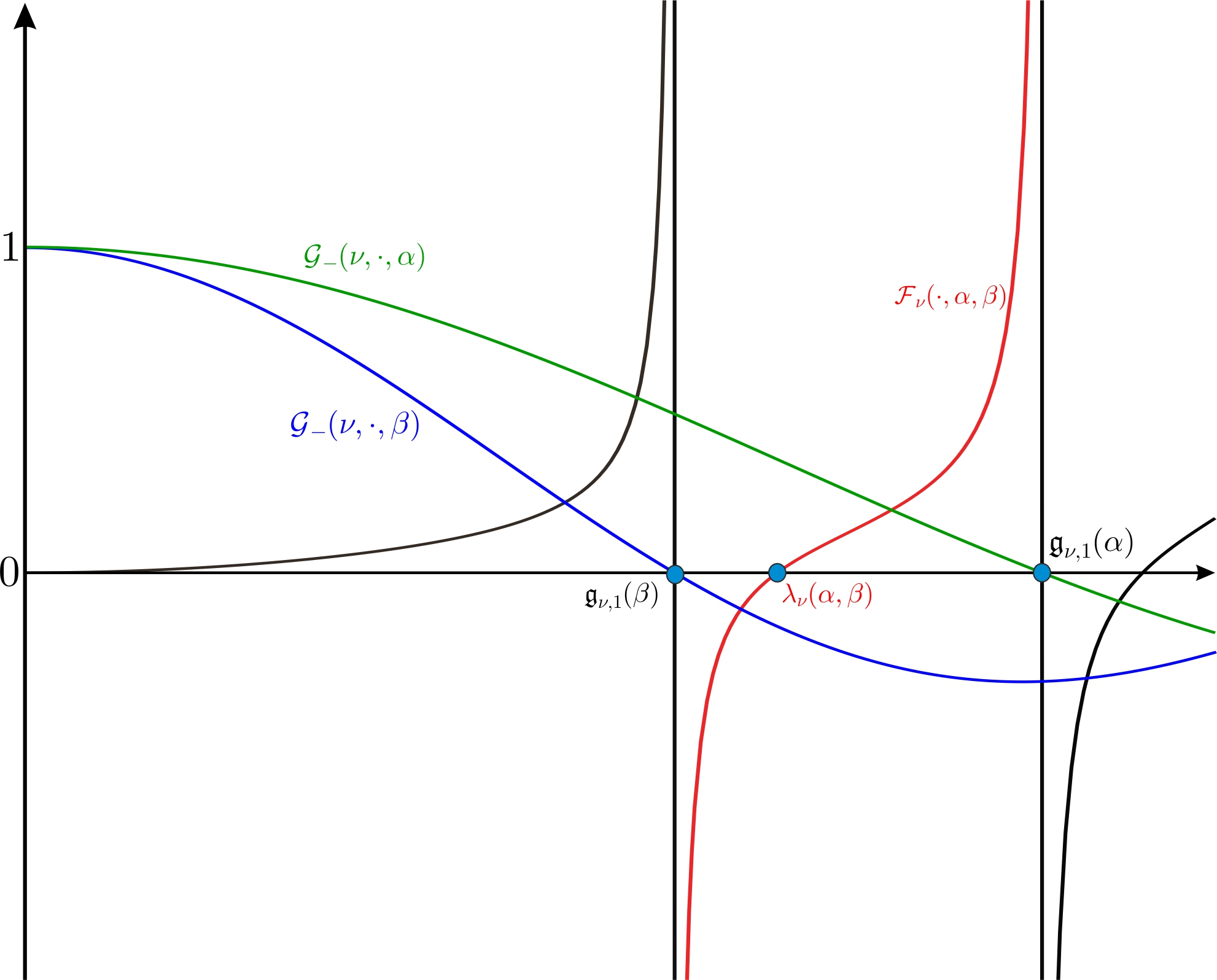
Due to (4.6) and Proposition 2.2/(iii), for every $\lambda>\frac{n-1}{2}\kappa$ the function $t\mapsto\mathcal{G}_{-}(\nu,\lambda,t)$ has infinitely many zeros; let $\mathfrak{g}_{\nu,k}(t)$ be the $k^{\rm th}$ zero of the functions $\mathcal{G}_{-}(\nu,\cdot,t)$ and respectively. Thus, $t\mapsto\mathcal{K}_{\nu}(\lambda,t)$ has infinitely many simple poles.

Let $L_{0}>0$ be fixed such that $2V_{\kappa}(L_{0})=V_{g}(\Omega)=V_{\kappa}(L)$, corresponding to the case $a=b=L_{0}$ in (3.20), and let $\tilde{L}_{0}=\sinh(\frac{\kappa L_{0}}{2})^{2}>0.$ Postponing the fact that $\lambda\mapsto\mathcal{K}_{\nu}(\lambda,t)$ is decreasing on $(0,\infty)$ between any two consecutive zeros of $\mathcal{G}_{-}(\nu,\cdot,t)$ (see Step 1 below for $\nu\in\{0,1/2\}$), and $\lim_{\lambda\to 0}\mathcal{K}_{\nu}(\lambda,t)=0$ for every $t>0$, the same properties hold for $\mathcal{F}_{\nu}(\cdot,\alpha,\beta)$ for any choice of $\alpha,\beta\geq 0$ verifying (4.2). Accordingly, the first positive zero $\lambda_{\nu}(\alpha,\beta)$ of $\mathcal{F}_{\nu}(\cdot,\alpha,\beta)$ will be situated between the poles of $\mathcal{F}_{\nu}(\cdot,\alpha,\beta)$; namely, if we assume without loss of generality that $\alpha\leq\beta,$ then

$$\mathfrak{g}_{\nu,1}(\beta)\leq\lambda_{\nu}(\alpha,\beta)\leq\min\{\mathfrak{g}_{\nu,1}(\alpha),\mathfrak{g}_{\nu,2}(\beta)\},$$ (5.4)

with the convention $\mathfrak{g}_{\nu,1}(0)=+\infty$. In the limiting case when $a$ and $b$ approach $L_{0}$ (thus, $\alpha$ and $\beta$ approach $\tilde{L}_{0}$), the latter relation implies that

$$\lambda_{\nu}(\tilde{L}_{0},\tilde{L}_{0})=\mathfrak{g}_{\nu,1}(\tilde{L}_{0}),$$

see Figure 1. Therefore, a necessary condition for the validity of (5.3) is to have

$$\mathfrak{g}_{\nu,1}(\tilde{L}_{0})\geq\lambda_{\nu}(0,\tilde{L}).$$ (5.5)

Figure 1. The first positive zero $\lambda_{\nu}(\alpha,\beta)$ of $\mathcal{F}_{\nu}(\cdot,\alpha,\beta)$ is between the poles $\mathfrak{g}_{\nu,1}(\beta)$ and $\mathfrak{g}_{\nu,1}(\alpha)$ of $\mathcal{F}_{\nu}(\cdot,\alpha,\beta)$; in particular, when $\alpha$ and $\beta$ approach to $\tilde{L}_{0}=\sinh(\frac{\kappa L_{0}}{2})^{2}$ (where $2V_{\kappa}(L_{0})=V_{g}(\Omega)$) it follows the limiting relation $\lambda_{\nu}(\tilde{L}_{0},\tilde{L}_{0})=\mathfrak{g}_{\nu,1}(\tilde{L}_{0}).$

Remark 5.1.

Inequality (5.5) fails for every choice of $L>0$ and $\kappa\geq 0$ whenever $n\geq 4$ (thus $\nu\in\{1,3/2,2,...\}$). However, (5.5) turns to be sufficient for the validity of (5.3) when

• either $\kappa=0$ and $n\in\{2,3\}$, corresponding to Ashbaugh and Benguria [1];

• or $\kappa>0$, $n\in\{2,3\}$ and $L>0$ is sufficiently small, see §5.2.

5.2. The $2$- and $3$-dimensional cases: proof of Theorem 1.2.

In the case $\kappa=0$, relation (5.5) reduces to $2^{\frac{1}{n}}j_{\nu,1}\geq\mathfrak{h}_{\nu}$, since $\mathfrak{g}_{\nu,1}(\tilde{L}_{0})=\tilde{L}_{0}^{-1}j_{\nu,1}$, $\lambda_{\nu}(0,\tilde{L}_{0})=\tilde{L}_{0}^{-1}\mathfrak{h}_{\nu}$, and $L_{0}=\tilde{L}_{0}=2^{-\frac{1}{n}}L=2^{-\frac{1}{n}}\tilde{L}.$ Clearly, inequality $2^{\frac{1}{n}}j_{\nu,1}\geq\mathfrak{h}_{\nu}$ holds only when $n\in\{2,3\}$, and (1.10) immediately follows by (3.19), (4.1) and the proof of Ashbaugh and Benguria [1], as we described in §5.1. In addition, (1.11) trivially holds since $\Gamma_{0}(B_{0}(L))=\frac{\mathfrak{h}_{\nu}^{4}}{L^{4}}$ for every $L>0.$

In the sequel, we assume that $\kappa>0$ and $n\in\{2,3\}$ (thus $\nu\in\{0,1/2\}$); the proof is divided into three steps.

Step 1: Monotonicity of $\mathcal{K}_{\nu}(\cdot,t)$ for $\nu\in\{0,1/2\}$. We start with the case $n=3$ ($\nu=1/2$); the key observation is that for every $\Lambda,t>0$, one has

$${\bf F}\left(\frac{1-i\Lambda}{2},\frac{1+i\Lambda}{2};\frac{3}{2};-t\right)=\frac{\sin(\Lambda\ln(\sqrt{t}+\sqrt{1+t}))}{\Lambda\sqrt{t}}$$

and

$${\bf F}\left(\frac{1-\Lambda}{2},\frac{1+\Lambda}{2};\frac{3}{2};-t\right)=\frac{\sinh(\Lambda\ln(\sqrt{t}+\sqrt{1+t}))}{\Lambda\sqrt{t}},$$

both reduction formulas following by relation (15.4.15) of Olver et al. [33]. Taking advantage of the latter reduction forms, one has that

$$\mathcal{G}_{-}(1/2,\lambda,t)=\left\{\begin{array}[]{lll}\frac{\sin(\tilde{\Lambda}_{-}\ln(\sqrt{t}+\sqrt{1+t}))}{\tilde{\Lambda}_{-}\sqrt{t}}&\mbox{if}&\lambda>\kappa;\\ \frac{\ln(\sqrt{t}+\sqrt{1+t})}{\sqrt{t}}&\mbox{if}&\lambda=\kappa;\\ \frac{\sinh(\Lambda_{-}\ln(\sqrt{t}+\sqrt{1+t}))}{\Lambda_{-}\sqrt{t}}&\mbox{if}&\lambda<\kappa,\\ \end{array}\right.\ \ {\rm and}\ \ \mathcal{G}_{+}(1/2,\lambda,t)=\frac{\sinh(\tilde{\Lambda}_{+}\ln(\sqrt{t}+\sqrt{1+t}))}{\tilde{\Lambda}_{+}\sqrt{t}},$$

where

$$\tilde{\Lambda}_{-}:=i\Lambda_{-}=2\sqrt{\frac{\lambda^{2}}{\kappa^{2}}-1}\ \ {\rm and}\ \ \tilde{\Lambda}_{+}:=\Lambda_{+}=2\sqrt{\frac{\lambda^{2}}{\kappa^{2}}+1}.$$ (5.6)

Thus, by (4.4) one has for every $t>0$ that

$$\mathcal{K}_{1/2}(\lambda,t)={\small\frac{1}{2\sqrt{t(1+t)}}\cdot\left\{\begin{array}[]{lll}{\tilde{\Lambda}_{-}\cot(\tilde{\Lambda}_{-}\ln(\sqrt{t}+\sqrt{1+t}))-\tilde{\Lambda}_{+}\coth(\tilde{\Lambda}_{+}\ln(\sqrt{t}+\sqrt{1+t}))}&\mbox{if}&\lambda>\kappa;\\ \frac{1}{\ln(\sqrt{t}+\sqrt{1+t})}-2\sqrt{2}\coth(2\sqrt{2}\ln(\sqrt{t}+\sqrt{1+t}))&\mbox{if}&\lambda=\kappa;\\ {\Lambda_{-}\coth(\Lambda_{-}\ln(\sqrt{t}+\sqrt{1+t}))-\tilde{\Lambda}_{+}\coth(\tilde{\Lambda}_{+}\ln(\sqrt{t}+\sqrt{1+t}))}&\mbox{if}&\lambda<\kappa.\\ \end{array}\right.}$$ (5.7)

Elementary computation guarantees that $\lambda\mapsto\mathcal{K}_{1/2}(\lambda,t)$ is decreasing on $(0,\infty)$ between any two consecutive zeros of $\mathcal{G}_{-}(1/2,\cdot,t)$ for every $t>0$ fixed; the zeros of $\mathcal{G}_{-}(1/2,\cdot,t)$ occur only beyond the value $\kappa$ and can be explicitly given by

$$\mathfrak{g}_{1/2,k}(t)=\kappa\sqrt{1+\left(\frac{k\pi}{2\ln(\sqrt{t}+\sqrt{1+t})}\right)^{2}},\ \ k\in\mathbb{N}.$$ (5.8)

In addition, since $\Lambda_{-}(0)=\Lambda_{+}(0)=2$, we also have $\lim_{\lambda\to 0}\mathcal{K}_{1/2}(\lambda,t)=0$ for every $t>0$. In particular, relation (5.4) is justified for $\nu=1/2$.

When $n=2$, the differentiation formula (2.5) and the connection formula (15.10.11) of Olver et al. [33] together with (4.4) give

$$\mathcal{K}_{0}(\lambda,t)=-\frac{\lambda^{2}}{\kappa^{2}(1+t)}\left(\frac{{\bf F}\left(\frac{1+\Lambda_{+}}{2},\frac{3+\Lambda_{+}}{2};2;\frac{t}{1+t}\right)}{{\bf F}\left(\frac{1+\Lambda_{+}}{2},\frac{1+\Lambda_{+}}{2};1;\frac{t}{1+t}\right)}+\frac{{\bf F}\left(\frac{1+\Lambda_{-}}{2},\frac{3+\Lambda_{-}}{2};2;\frac{t}{1+t}\right)}{{\bf F}\left(\frac{1+\Lambda_{-}}{2},\frac{1+\Lambda_{-}}{2};1;\frac{t}{1+t}\right)}\right),\ \ \lambda,t>0,$$ (5.9)

where $\Lambda_{\pm}=\sqrt{1\pm 4\frac{\lambda^{2}}{\kappa^{2}}}$ is from (4.3). It is clear that $\lim_{\lambda\to 0}\mathcal{K}_{0}(\lambda,t)=0$ for every $t>0$. By using the definition (2.3) of the hypergeometric functions and the continued fraction representation, see Cuyt et al. [17, Chapter 15](15.7.5) and Olver et al. [33], a long computation shows that for every fixed $t>0$ the function $\lambda\mapsto\mathcal{K}_{0}(\lambda,t)$ is decreasing on $(0,\infty)$ between any two consecutive zeros of $\mathcal{G}_{-}(0,\cdot,t)$; see also Karp [24].

Step 2: Admissible range for $L>0$ in (5.5). We are going to prove that (5.5) holds for small $L>0$. We first give a crucial asymptotic estimate for $\lambda_{\nu}(0,\tilde{L})$ when $L\ll 1$, i.e. assume that

$${\lambda_{\nu}(0,\tilde{L})}\sim\kappa\sqrt{\frac{(n-1)^{2}}{4}+\frac{C^{2}}{L^{2}}}\ \ {\rm as}\ \ L\to 0,$$ (5.10)

for some $C>0,$ where $\tilde{L}=\sinh(\frac{\kappa L}{2})^{2}$; our computations are valid for every $\nu\in\{0,1/2,1,...\}$. We observe that for every $k\in\mathbb{N}$ one has

$$\lim_{L\to 0}\left(\frac{1}{2}-i\frac{C}{L}\right)_{k}\left(\frac{1}{2}+i\frac{C}{L}\right)_{k}\sinh^{2k}\left(\frac{\kappa L}{2}\right)=\left(\frac{C\kappa}{2}\right)^{2k}.$$

Thus, by (5.10) and uniform-convergence reasons, the latter limit implies that

$\lim_{L\to 0}\mathcal{G}_{-}(\nu,\lambda_{\nu}(0,\tilde{L}),\tilde{L})=$

$$= \lim_{L\to 0}{\bf F}\left(\frac{1-i\sqrt{4\frac{{\lambda^{2}_{\nu}(0,\tilde{L})}}{\kappa^{2}}-(n-1)^{2}}}{2},\frac{1+i\sqrt{4\frac{{\lambda^{2}_{\nu}(0,\tilde{L})}}{\kappa^{2}}-(n-1)^{2}}}{2};\frac{n}{2};-\sinh^{2}\left(\frac{\kappa L}{2}\right)\right)$$

$$= \sum_{k\geq 0}\frac{(-1)^{k}}{k!\left(\frac{n}{2}\right)_{k}}\left(\frac{C\kappa}{2}\right)^{2k}$$

$$= \frac{\Gamma\left(\frac{n}{2}\right)}{\left(\frac{C\kappa}{2}\right)^{\nu}}J_{\nu}(C\kappa).$$

In a similar way, it turns out that

$$\lim_{L\to 0}\mathcal{G}_{+}(\nu,\lambda_{\nu}(0,\tilde{L}),\tilde{L}) = \sum_{k\geq 0}\frac{1}{k!\left(\frac{n}{2}\right)_{k}}\left(\frac{C\kappa}{2}\right)^{2k}=\frac{\Gamma\left(\frac{n}{2}\right)}{\left(\frac{C\kappa}{2}\right)^{\nu}}I_{\nu}(C\kappa).$$

Moreover, the differentiation formula (2.5) provides

$$\lim_{L\to 0}L^{2}\mathcal{G}_{-}^{\prime}(\nu,\lambda_{\nu}(0,\tilde{L}),\tilde{L})=C^{2}\frac{\Gamma\left(\frac{n}{2}+1\right)}{\left(\frac{C\kappa}{2}\right)^{\nu+1}}J_{\nu+1}(C\kappa)$$

and

$$\lim_{L\to 0}L^{2}\mathcal{G}_{+}^{\prime}(\nu,\lambda_{\nu}(0,\tilde{L}),\tilde{L})=-C^{2}\frac{\Gamma\left(\frac{n}{2}+1\right)}{\left(\frac{C\kappa}{2}\right)^{\nu+1}}I_{\nu+1}(C\kappa).$$

Since by definition $\mathcal{K}_{\nu}({\lambda_{\nu}(0,\tilde{L})},\tilde{L})=0$, the above four limits imply that

$$\frac{J_{\nu+1}(C\kappa)}{J_{\nu}(C\kappa)}+\frac{I_{\nu+1}(C\kappa)}{I_{\nu}(C\kappa)}=0.$$

Accordingly, we immediately have that $C\kappa=\mathfrak{h}_{\nu},$ obtaining

$${\lambda_{\nu}(0,\tilde{L})}\sim\sqrt{\frac{(n-1)^{2}}{4}\kappa^{2}+\frac{\mathfrak{h}_{\nu}^{2}}{L^{2}}}\ \ {\rm as}\ \ L\to 0,$$ (5.11)

which is precisely (1.11).

We now provide some estimates for $\mathfrak{g}_{\nu,1}(\tilde{L}_{0})$ for $\nu\in\{0,1/2\}$ whenever $L_{0}\to 0$. Incidentally, it turns out that for $n=2$ ($\nu=0$), the function $t\mapsto\mathcal{G}_{-}(0,\lambda,t):={\bf F}\left(\frac{1-\Lambda_{-}}{2},\frac{1+\Lambda_{-}}{2};1;-t\right)$ appears as the extremal in the second-order Rayleigh problem (for membranes) on the geodesic ball $B_{\kappa}(L_{0})$ with the initial condition ${\bf F}\left(\frac{1-\Lambda_{-}}{2},\frac{1+\Lambda_{-}}{2};1;-\tilde{L}_{0}\right)=0$ where $\tilde{L}_{0}=\sinh(\frac{\kappa L_{0}}{2})^{2}$, see e.g. Kristály [29], while the first eigenvalue $\gamma_{g}(B_{\kappa}(L_{0}))$ corresponding to (1.6) on $B_{\kappa}(L_{0})$ is precisely $\mathfrak{g}_{0,1}(\tilde{L}_{0})$. Therefore, by Chavel [8, p.318] one has that

$$\mathfrak{g}_{0,1}(\tilde{L}_{0})=\gamma_{g}(B_{\kappa}(L_{0}))\sim\sqrt{\frac{1}{3}\kappa^{2}+\left(\frac{j_{0,1}}{L_{0}}\right)^{2}}\ \ {\rm as}\ \ L_{0}\to 0.$$ (5.12)

For $n=3$ (thus $\nu=1/2$), since $j_{1/2,1}=\pi$, we also have by (5.8) that

$$\mathfrak{g}_{1/2,1}(\tilde{L}_{0})=\sqrt{\kappa^{2}+\left(\frac{j_{1/2,1}}{\kappa L_{0}}\right)^{2}}\ \ \ {\rm for\ all}\ L_{0}>0.$$ (5.13)

Recalling $2V_{\kappa}(L_{0})=V_{\kappa}(L)$, it follows that $L_{0}\sim 2^{-\frac{1}{n}}L$ whenever $L\ll 1.$ Now, by combining these facts together with (5.12) and (5.13), it follows that

$$\liminf_{L\to 0}\frac{\mathfrak{g}_{\nu,1}(\tilde{L}_{0})}{\lambda_{\nu}(0,\tilde{L})}=\left\{\begin{array}[]{lll}\frac{2^{\frac{1}{2}}j_{0,1}}{\mathfrak{h}_{0}}\approx\frac{2^{\frac{1}{2}}\cdot 2.4048}{3.19622}\approx 1.064>1&\mbox{if}&n=2,\\ \\ \frac{2^{\frac{1}{3}}j_{1/2,1}}{\mathfrak{h}_{1/2}}\approx\frac{2^{\frac{1}{3}}\pi}{3.9266}\approx 1.008>1&\mbox{if}&n=3,\end{array}\right.$$ (5.14)

thus verifying (5.5) for sufficiently small $L>0.$

Numerical tests show that (5.5) fails for large values of $L>0$ whenever $n\in\{2,3\}$; in the sequel we provide the precise proof for $n=3$. By $2V_{\kappa}(L_{0})=V_{\kappa}(L)$ we observe that $L_{0}\sim L-\frac{\ln 2}{2\kappa}$ whenever $L\gg 1;$ in particular, (5.13) shows that $\mathfrak{g}_{1/2,1}(\tilde{L}_{0})\in(\mathfrak{g}_{1/2,1}(\tilde{L}),\mathfrak{g}_{1/2,2}(\tilde{L})).$ Making use of (5.7) and (5.13), the latter estimate implies that

$$\liminf_{L\to\infty}\mathcal{K}_{1/2}(\mathfrak{g}_{1/2,1}(\tilde{L}_{0}),\tilde{L})=2\left(\frac{1}{\ln(2)}-\sqrt{2}\right)\approx 0.0569>0.$$ (5.15)

If (5.5) would be true for $L\gg 1,$ relation (5.15), the monotonicity of $\mathcal{K}_{1/2}(\cdot,\tilde{L})$ in the interval $(\mathfrak{g}_{1/2,1}(\tilde{L}),\mathfrak{g}_{1/2,2}(\tilde{L}))$, see Step 1, and the fact that ${\lambda_{1/2}(0,\tilde{L})}\in(\mathfrak{g}_{1/2,1}(\tilde{L}),\mathfrak{g}_{1/2,2}(\tilde{L}))$, see (5.4), imply that

$$0<\mathcal{K}_{1/2}(\mathfrak{g}_{1/2,1}(\tilde{L}_{0}),\tilde{L})\leq\mathcal{K}_{1/2}({\lambda_{1/2}(0,\tilde{L})},\tilde{L})=0,$$

a contradiction.

We now provide the approximate threshold values of $L$ when such turnouts occur for $n=2$ and $n=3$, respectively. Numerical approximations show that (5.5) holds for $n=2$ whenever $0<L<\frac{2.1492}{\kappa}=:l_{2}$ and for $n=3$ whenever $0<L<\frac{0.719}{\kappa}=:l_{3}$, see Figure 2.

Figure 2. For $n\in\{2,3\}$ the admissible range is $0<L<l_{n}$ with $l_{2}=\frac{2.1492}{\kappa}$ and $l_{3}=\frac{0.719}{\kappa}$, respectively; for large values of $L$ inequality (5.5) fails.

Due to its empirical nature, the latter values are not precise, but inequality (5.5) fails for any larger values than $L=\frac{2.1493}{\kappa}$ whenever $n=2$ and $L=\frac{0.72}{\kappa}$ whenever $n=3$, respectively. Accordingly, since $V_{g}(\Omega)=V_{\kappa}(L)$, the volume of $\Omega\subset M$ cannot exceed

$$V_{\kappa}(l_{n})=n\omega_{n}\int_{0}^{l_{n}}{\mathbf{s}}_{\kappa}(\rho)^{n-1}{\rm d}\rho\approx\left\{\begin{array}[]{lll}2\pi\frac{3.34728}{\kappa^{2}}\approx\frac{21.031}{\kappa^{2}}&\mbox{if}&n=2,\\ \\ 4\pi\frac{0.137}{\kappa^{3}}\approx\frac{1.721}{\kappa^{3}}&\mbox{if}&n=3,\end{array}\right.$$ (5.16)

which appear in the statement of the theorem.

Step 3: Concluding the proof of (1.10). Without mentioning explicitly, we assume in the sequel that $\alpha,\beta\geq 0$ verify (4.2) and $\alpha\leq\beta$. Furthermore, without loss of generality, we may consider the case when strict inequality occurs in (5.5). Since $\lambda_{\nu}(\tilde{L}_{0},\tilde{L}_{0})=\mathfrak{g}_{{\nu},1}(\tilde{L}_{0})>\lambda_{\nu}(0,\tilde{L}),$ by continuity reasons in (4.5), it turns out that $\lambda_{{\nu}}(\alpha,\beta)>\lambda_{{\nu}}(0,\tilde{L})$ for $\alpha>0$ sufficiently close to $\tilde{L}_{0}$. More precisely, the full range of $\alpha$ with this property is $[\alpha_{0},\tilde{L}_{0}]$ where $\alpha_{0},\beta_{0}$ verify (4.2) and $\beta_{0}$ is the first positive value such that $\lambda_{{\nu}}(0,\tilde{L})=\mathfrak{g}_{{\nu},1}(\beta_{0})$, i.e. the first positive zero of $\mathcal{G}_{-}({\nu},\lambda_{{\nu}}(0,\tilde{L}),\cdot)$, being a pole of $\mathcal{F}_{{\nu}}(\lambda_{{\nu}}(0,\tilde{L}),\cdot,\cdot)$, see Figure 3.

Figure 3. Continuity reason (when $\alpha\in[\alpha_{0},\tilde{L}_{0}]$) and monotonicity argument for $\mathcal{F}_{\nu}$ (when $\alpha\in(0,\alpha_{0})$) imply that $\lambda_{{\nu}}(\alpha,\beta)>\lambda_{{\nu}}(0,\tilde{L})$.

We claim that for every $\alpha\in(0,\alpha_{0})$, one has

$$\mathcal{F}_{\nu}(\lambda_{\nu}(0,\tilde{L}),\alpha,\beta)>0.$$ (5.17)

We immediately observe that $\mathcal{F}_{\nu}(\lambda_{\nu}(0,\tilde{L}),0,\tilde{L})=0$ and $\displaystyle\lim_{\alpha\to\alpha_{0}^{-}}\mathcal{F}_{\nu}(\lambda_{\nu}(0,\tilde{L}),\alpha,\beta)=+\infty.$ In order to check (5.17) one can prove that $\alpha\mapsto\mathcal{F}_{\nu}(\lambda_{\nu}(0,\tilde{L}),\alpha,\beta(\alpha))$ is increasing on $(0,\alpha_{0}),$ where $\beta=\beta(\alpha)$ is given by (4.2). We notice that $\beta^{\prime}(\alpha)=-1$ (since $\alpha+\beta=\tilde{L}$) when $n=2$ and $\sqrt{\alpha(1+\alpha)}+\beta^{\prime}(\alpha)\sqrt{\beta(1+\beta)}=0$ when $n=3$. Therefore, since $\mathcal{F}_{\nu}$ contains ratios of hypergeometric functions, a similar monotonicity argument as in Karp and Sitnik [25] implies that

$$\frac{\rm d}{\rm d\alpha}\mathcal{F}_{\nu}(\lambda_{\nu}(0,\tilde{L}),\alpha,\beta(\alpha))>0,\ \ \alpha\in(0,\alpha_{0}).$$

Now, if there exists $\alpha\in(0,\alpha_{0})$ such that $\lambda_{{\nu}}(\alpha,\beta)<\lambda_{{\nu}}(0,\tilde{L})$, the fact that $\mathcal{F}_{\nu}(\cdot,\alpha,\beta)$ is decreasing (cf. Step 1) and relation (5.17) imply that

$$0<\mathcal{F}_{\nu}(\lambda_{\nu}(0,\tilde{L}),\alpha,\beta)\leq\mathcal{F}_{\nu}(\lambda_{\nu}(\alpha,\beta),\alpha,\beta)=0,$$

a contradiction, which concludes the proof of (5.3), so (1.10).

If equality occurs in (1.10) then we necessarily have equality in (3.13) (relation (3.14) being canceled, or vice-versa). In particular, for a.e. $t>0$ we also have equality in (3.17), which implies equality in the isoperimetric inequality. According to the equality case in the $\kappa$-Cartan-Hadamard conjecture, the sets $\{x\in\Omega:u_{+}(x)>t\}$ and $\{x\in N_{\kappa}^{n}:u_{+}^{\star}(x)>t\}$ are isometric for a.e. $t>0$; in particular, $\Omega\subset M$ is isometric to the ball $\Omega^{\star}=B_{\kappa}(L)\subset\mathbb{H}_{-\kappa^{2}}^{n}$. The converse is trivial.

We conclude this subsection by showing the accuracy of the asymptotic estimate (1.11) (see also relation (5.11) in Step 2) of the fundamental tone $\Gamma_{\kappa}(B_{\kappa}(L))$ for $L\ll 1$ in 2- and 3-dimensions; by scaling reasons, we present the values $\Gamma_{\kappa}(B_{\kappa}(L))^{1/4}$.

$L$	$n=2$ $(\nu=0)$		$n=3$ $(\nu=1/2)$
	Algebraic value of $\Gamma_{\kappa}(B_{\kappa}(L))^{1/4}$	Approximate value of $\Gamma_{\kappa}(B_{\kappa}(L))^{1/4}$	Algebraic value of $\Gamma_{\kappa}(B_{\kappa}(L))^{1/4}$	Approximate value of $\Gamma_{\kappa}(B_{\kappa}(L))^{1/4}$
$0.7$	4.5908	4.5728	5.6761	5.6978
$0.1$	31.9657	31.9631	39.2755	39.2787
$0.05$	63.9262	63.9248	78.5368	78.5383
$0.003$	1065.4069	1065.4066	1308.8677	1308.8670

Table 1. Comparison of the algebraic and approximate values of the fundamental tone $\Gamma_{\kappa}(B_{\kappa}(L))$ for some small values of $L>0$; the algebraic value of $\Gamma_{\kappa}(B_{\kappa}(L))$ is $\lambda^{4}$ where $\lambda>0$ is the first positive root of $\mathcal{K}_{\nu}\left(\lambda,\sinh(\frac{\kappa L}{2})^{2}\right)=0$, while the approximate value of $\Gamma_{\kappa}(B_{\kappa}(L))$ is given by (1.11). For simplicity, $\kappa=1$.

5.3. Proof of (1.8) and (1.9)

We distinguish two cases.

Case 1: $n=3$. Let $L>0.$ Applying (5.4) for $\alpha=0$ and $\beta=\tilde{L}=\sinh(\frac{\kappa L}{2})^{2}$ and using (5.8), it turns out that

$$\kappa\sqrt{1+\left(\frac{\pi}{\kappa L}\right)^{2}}\leq\lambda_{1/2}(0,\tilde{L})\leq\kappa\sqrt{1+\left(\frac{2\pi}{\kappa L}\right)^{2}}.$$ (5.18)

Therefore,

$$\lim_{L\to\infty}\Gamma_{\kappa}(B_{\kappa}(L))=\lim_{L\to\infty}\lambda_{1/2}^{4}(0,\tilde{L})=\kappa^{4},$$

which proves (1.8) for $n=3$.

Case 2: $n=2$. Although we have no a similar relation as (5.8), we can establish its approximate version for $n=2$. We recall (see Step 2 from §5.2) that the zeros of

$${\bf F}\left(\frac{1-\sqrt{1-\frac{4\lambda^{2}}{\kappa^{2}}}}{2},\frac{1+\sqrt{1-\frac{4\lambda^{2}}{\kappa^{2}}}}{2};1;-\tilde{L}\right)=0$$

are the values $\mathfrak{g}_{0,k}(\tilde{L})$, $k\in\mathbb{N}$, and the first eigenvalue $\gamma_{g}(B_{\kappa}(L))$ corresponding to (1.6) on $B_{\kappa}(L)$ is $\mathfrak{g}_{0,1}^{2}(\tilde{L})$, where $\tilde{L}=\sinh(\frac{\kappa L}{2})^{2}$. Since $\mathfrak{g}_{0,k}(\tilde{L})>\frac{\kappa}{2}$, see (1.6), let $\gamma_{k}:=\sqrt{\frac{\mathfrak{g}_{0,k}(\tilde{L})^{2}}{\kappa^{2}}-\frac{1}{4}}\in\mathbb{R}$ and recall that

$${\bf F}\left(\frac{1}{2}-i\gamma_{k},\frac{1}{2}+i\gamma_{k};1;-\sinh\left(\frac{\kappa L}{2}\right)^{2}\right)={\bf P}_{-\frac{1}{2}+i\gamma_{k}}(\cosh(\kappa L)),$$

where ${\bf P}_{-\frac{1}{2}+i\gamma_{k}}$ stands for the spherical Legendre function, see Robin [37], Zhurina and Karmazina [41]. By an integral representation of the spherical Legendre function, it turns out that for large $L>0$,

$$\kappa L\gamma_{k}\sim k\pi-\arctan(v_{k}/u_{k}),\ \ k\in\mathbb{N},$$

where

$$v_{k}=\int_{0}^{\infty}\frac{\sin(\gamma_{k}y)}{\sqrt{e^{y}-1}}{\rm d}y\ \ {\rm and}\ \ u_{k}=\int_{0}^{\infty}\frac{\cos(\gamma_{k}y)}{\sqrt{e^{y}-1}}{\rm d}y,$$

see Zhurina and Karmazina [41, p. 24-25]. In particular, $\gamma_{k}\sim\frac{k\pi}{\kappa L}$ as $L\gg 1$ for every $k\in\mathbb{N}$. Combining these facts, we have for every $k\in\mathbb{N}$ that

$$\mathfrak{g}_{0,k}(\tilde{L})\sim\kappa\sqrt{\frac{1}{4}+\left(\frac{k\pi}{\kappa L}\right)^{2}}\ \ \ {\rm for}\ \ L\gg 1.$$ (5.19)

By using again (5.4) for $\alpha=0$ and $\beta=\tilde{L}=\sinh(\frac{\kappa L}{2})^{2}$, relation (5.19) provides

$$\kappa\sqrt{\frac{1}{4}+\left(\frac{\pi}{\kappa L}\right)^{2}}\leq\lambda_{0}(0,\tilde{L})\leq\kappa\sqrt{\frac{1}{4}+\left(\frac{2\pi}{\kappa L}\right)^{2}}\ \ \ \ {\rm for}\ \ L\gg 1.$$

Therefore,

$$\lim_{L\to\infty}\Gamma_{\kappa}(B_{\kappa}(L))=\lim_{L\to\infty}\lambda_{0}^{4}(0,\tilde{L})=\frac{\kappa^{4}}{16},$$

which concludes the proof of (1.8) for $n=2$.

We now prove (1.9). In particular, by (1.8) we have for $n\in\{2,3\}$ that

$$\lim_{L\to\infty}\Gamma_{\kappa}^{1}(B_{\kappa}(L))=\lim_{L\to\infty}\Gamma_{\kappa}(B_{\kappa}(L))=\frac{(n-1)^{4}}{16}\kappa^{4}.$$

Since $\{\Gamma_{\kappa}^{l}(\Omega)\}_{l}$ is a nondecreasing sequence which is bounded from below by $\frac{(n-1)^{4}}{16}\kappa^{4}$ (see Proposition 4.1), the estimate of Cheng and Yang [12], i.e.

$$\Gamma_{\kappa}^{l+1}(B_{\kappa}(L))-\frac{(n-1)^{4}}{16}\kappa^{4}\leq 25l^{12}\left(\Gamma_{\kappa}^{1}(B_{\kappa}(L))-\frac{(n-1)^{4}}{16}\kappa^{4}\right)\ \ {\rm for\ all}\ \ l\in\mathbb{N},$$

provides the required statement (1.9). $\square$

Remark 5.2.

(a) The precise values of $\mathfrak{g}_{1/2,k}(\tilde{L})$ and the approximative values of $\mathfrak{g}_{0,k}(\tilde{L})$ are crucial in the proof of (1.8), respectively. The involved form of $\mathcal{K}_{\nu}(\lambda,t)$ for $\nu\in\{1,3/2,...\}$ (i.e. $n\geq 4$) implies several technical difficulties to perform similar asymptotic estimates as above; however, we still believe such estimates are valid in high-dimensions.

(b) When $n=3$, one can give an alternative proof of (1.8). To do this, note that

$$\Gamma_{\kappa}(B_{\kappa}(L))\leq\min_{v}\frac{\displaystyle\int_{B_{\kappa}(L)}(\Delta_{\kappa}v)^{2}{\rm d}v_{\kappa}}{\displaystyle\int_{B_{\kappa}(L)}v^{2}{\rm d}v_{\kappa}}=:c_{\kappa}(L),$$ (5.20)

where $v\in W^{2,2}_{0}(B_{\kappa}(L))\setminus\{0\}$ is taken over of all radially symmetric functions. A variational argument similar to the one developed in §4 shows that $c_{\kappa}(L)=\lambda^{4}$ where $\lambda>0$ is the first positive root of the transcendental equation

$${\tilde{\Lambda}_{-}\cot\left(\tilde{\Lambda}_{-}\frac{\kappa L}{2}\right)-\tilde{\Lambda}_{+}\coth\left(\tilde{\Lambda}_{+}\frac{\kappa L}{2}\right)}=0,$$ (5.21)

see (5.7), where $\tilde{\Lambda}_{-}$ and $\tilde{\Lambda}_{+}$ come from (5.6). Analogously to (5.10), assume that

$$c_{\kappa}(L)\sim\kappa^{4}\left({1+\frac{D^{2}}{L^{2}}}\right)^{2}\ \ {\rm as}\ \ L\to\infty,$$ (5.22)

for some $D>0.$ Inserting (5.22) into (5.21) and letting $L\to\infty$, a simple computation yields that $\tan(\kappa D)=0$, i.e. $\kappa D=\pi$. We remark that (5.22) with $D=\frac{\pi}{\kappa}$ is in a perfect concordance with (5.18); Table 2 shows its accuracy (for $\kappa=1$).

$L$	Algebraic value of $\Gamma_{\kappa}(B_{\kappa}(L))^{1/4}$	Approximate value of $\Gamma_{\kappa}(B_{\kappa}(L))^{1/4}$
$50$	1+3.1908$\cdot 10^{-3}$	1+3.0795$\cdot 10^{-3}$
$100$	1+5.0041$\cdot 10^{-4}$	1+4.9335$\cdot 10^{-4}$
$5000$	1+1.9745$\cdot 10^{-7}$	1+1.9739$\cdot 10^{-7}$
$100000$	1+4.71$\cdot 10^{-10}$	1+4.9348$\cdot 10^{-10}$

Table 2. Comparison of the algebraic and approximate values of the fundamental tone $\Gamma_{\kappa}(B_{\kappa}(L))$ for some large values of $L>0$ in $3$-dimension; the algebraic value of $\Gamma_{\kappa}(B_{\kappa}(L))$ is $\lambda^{4}$ where $\lambda>0$ is the first positive root of $\mathcal{K}_{1/2}\left(\lambda,\sinh(\frac{\kappa L}{2})^{2}\right)=0$, while the approximate value of $\Gamma_{\kappa}(B_{\kappa}(L))$ is given by (5.22). For simplicity, $\kappa=1$.

5.4. Fundamental tones in high-dimensions: nonoptimal estimates.

Our argument cannot provide sharp comparison principles for fundamental tones since inequality (5.5) fails for any choice of $\kappa\geq 0$ and $L>0$ in the $n$-dimensional case whenever $n\geq 4$; we notice that similar phenomenon occurs also in the Euclidean setting, see Ashbaugh and Benguria [1]. However, in the case $\kappa=0$ we can provide some weak comparison principles. To this end, if $(M,g)$ is an $n$-dimensional $(n\geq 4)$ Cartan-Hadamard manifold and $\Omega\subset M$ a bounded domain with smooth boundary, a closer inspection of the proof – based on the validity of the $0$-Cartan-Hadamard conjecture proved by Ghomi and Spruck [20] – gives that

$$\Gamma_{g}(\Omega)\geq R^{0}_{\nu,a,b}\geq D_{n}\Gamma_{0}(\Omega^{\star}),$$ (5.23)

where $D_{n}=2^{\frac{4}{n}}\left(\frac{j_{\nu,1}}{\mathfrak{h}_{\nu}}\right)^{4}$ is the constant of Ashbaugh and Laugesen [2, Theorem 4]. Although $\displaystyle\lim_{n\to\infty}D_{n}=1$, the estimate (5.23) is not sharp since $D_{n}<1$ for every $n\geq 4$.

6. Application: proof of Theorem 1.3

Proof of (i). Assume that $\mu=0$ and $({\mathcal{P}})$ has a nonzero solution $u\in W_{0}^{2,2}(B_{\kappa}(L))\setminus\{0\}$, i.e.

$$\Delta_{\kappa}^{2}u+\gamma u=u^{p-1}\ \ {\rm in}\ \ B_{\kappa}(L).$$ (6.1)

Making use of the equation (4.10), it turns out that the function $v(x)=v(|x|)$ given by

$$v(r)=A\mathcal{G}_{+}\left(0,\lambda,\frac{r^{2}}{1-r^{2}}\right)+B\mathcal{G}_{-}\left(0,\lambda,\frac{r^{2}}{1-r^{2}}\right),\ r\in[0,\tanh(\kappa L/2)],$$

see (4.13), is a classical solution to

$$\Delta_{\kappa}^{2}v=\Gamma_{\kappa}(B_{k}(L))v\ \ {\rm in}\ \ B_{\kappa}(L),$$ (6.2)

while a suitable choice of the parameters $A$ and $B$ guarantees that $v\in W_{0}^{2,2}(B_{\kappa}(L))$ and $v>0$ in $B_{\kappa}(L)$, respectively. Multiplication of the equations (6.1) and (6.2) by $v>0$ and $u\geq 0$, respectively, and integrations by parts give that

$$\int_{B_{\kappa}(L)}\Delta_{\kappa}u\Delta_{\kappa}v{\rm d}v_{\kappa}+\gamma\int_{B_{\kappa}(L)}uv{\rm d}v_{\kappa}=\int_{B_{\kappa}(L)}u^{p-1}v{\rm d}v_{\kappa},$$

and

$$\int_{B_{\kappa}(L)}\Delta_{\kappa}v\Delta_{\kappa}u{\rm d}v_{\kappa}=\Gamma_{\kappa}(B_{k}(L))\int_{B_{\kappa}(L)}vu{\rm d}v_{\kappa}.$$

Therefore, one has

$$\left(\gamma+\Gamma_{\kappa}(B_{k}(L))\right)\int_{B_{\kappa}(L)}vu{\rm d}v_{\kappa}=\int_{B_{\kappa}(L)}u^{p-1}v{\rm d}v_{\kappa}>0,$$

which immediately implies that $\gamma>-\Gamma_{\kappa}(B_{k}(L)).$

Proof of (ii). Let us assume that $\mu>0$ and $\gamma>-\Gamma_{\kappa}(B_{k}(L)),$ and define the positive numbers

$$c_{\mu,\gamma}=\min\left(\mu,\frac{\min(\gamma,0)+\Gamma_{\kappa}(B_{k}(L))}{1+\Gamma_{\kappa}(B_{k}(L))}\right)\ \ {\rm and}\ \ C_{\mu,\gamma}=\max\{1,\mu,|\gamma|\}.$$

If $\mathcal{T}_{\mu,\gamma}:W_{0}^{2,2}(B_{\kappa}(L))\to\mathbb{R}$ is defined by

$$\mathcal{T}_{\mu,\gamma}(u)=\int_{B_{\kappa}(L)}\left((\Delta_{\kappa}u)^{2}+\mu|\nabla_{k}u|^{2}+\gamma u^{2}\right){\rm d}v_{\kappa},$$

then we have for every $u\in W_{0}^{2,2}(B_{\kappa}(L))$ that

$$c_{\mu,\gamma}\int_{B_{\kappa}(L)}\left((\Delta_{\kappa}u)^{2}+|\nabla_{k}u|^{2}+u^{2}\right){\rm d}v_{\kappa}\leq\mathcal{T}_{\mu,\gamma}(u)\leq C_{\mu,\gamma}\int_{B_{\kappa}(L)}\left((\Delta_{\kappa}u)^{2}+|\nabla_{k}u|^{2}+u^{2}\right){\rm d}v_{\kappa},$$

where the key ingredients are relations (5.16) and (1.10), respectively. Therefore, $u\mapsto\mathcal{T}_{\mu,\gamma}^{\frac{1}{2}}(u)$ defines a norm on $W_{0}^{2,2}(B_{\kappa}(L))$, equivalent to the usual one, see the proof of Proposition 3.1.

Let $h,H:\mathbb{R}\to[0,\infty)$ be defined by $h(t)=t_{+}^{p-1}$ and $H(t)=\frac{t_{+}^{p}}{p},$ where $t_{+}=\max(t,0)$ and associate with problem $({\mathcal{P}})$ its energy functional $\mathcal{E}_{\mu,\gamma}:W_{0}^{2,2}(B_{\kappa}(L))\to\mathbb{R}$ defined by

$$\mathcal{E}_{\mu,\gamma}(u)=\frac{1}{2}\mathcal{T}_{\mu,\gamma}(u)-\int_{B_{\kappa}(L)}H(u){\rm d}v_{\kappa}.$$

One can prove in a standard way that $\mathcal{E}_{\mu,\gamma}\in C^{1}(W_{0}^{2,2}(B_{\kappa}(L));\mathbb{R})$ and its differential is

$$\mathcal{E}_{\mu,\gamma}^{\prime}(u)(w)=\frac{1}{2}\mathcal{T}_{\mu,\gamma}^{\prime}(u)(w)-\int_{B_{\kappa}(L)}h(u)w{\rm d}v_{\kappa}\ \ {\rm for\ all}\ \ u,w\in W_{0}^{2,2}(B_{\kappa}(L)).$$

We prove that $\mathcal{E}_{\mu,\gamma}$ satisfies the Palais-Smale condition on $W_{0}^{2,2}(B_{\kappa}(L))$. To this end, let $\{u_{l}\}_{l}\subset W_{0}^{2,2}(B_{\kappa}(L))$ be a sequence verifying $\mathcal{E}_{\mu,\gamma}^{\prime}(u_{l})\to 0$ as $l\to\infty$ and $|\mathcal{E}_{\mu,\gamma}(u_{l})|\leq C$ ($l\in\mathbb{N}$) for some $C>0.$ The latter assumptions and relation

$$p\mathcal{E}_{\mu,\gamma}(u_{l})-\mathcal{E}_{\mu,\gamma}^{\prime}(u_{l})(u_{l})=\frac{p}{2}\mathcal{T}_{\mu,\gamma}(u_{l})-\frac{1}{2}\mathcal{T}_{\mu,\gamma}^{\prime}(u_{l})(u_{l})\equiv\left(\frac{p}{2}-1\right)\mathcal{T}_{\mu,\gamma}(u_{l}),\ \ l\in\mathbb{N},$$

immediately implies that $\{u_{l}\}_{l}$ is bounded in $W_{0}^{2,2}(B_{\kappa}(L))$; thus we may extract a subsequence of $\{u_{l}\}_{l}$ (denoted in the same way) which weakly converges to an element $u\in W_{0}^{2,2}(B_{\kappa}(L)).$ We notice that

$$\mathcal{T}_{\mu,\gamma}(u_{l}-u)=\mathcal{E}_{\mu,\gamma}^{\prime}(u_{l})(u_{l}-u)-\mathcal{E}_{\mu,\gamma}^{\prime}(u)(u_{l}-u)+\int_{B_{\kappa}(L)}(h(u_{l})-h(u))(u_{l}-u){\rm d}v_{\kappa},\ \ l\in\mathbb{N}.$$

Using the fact that $\mathcal{E}_{\mu,\gamma}^{\prime}(u_{l})\to 0$ as $l\to\infty$ and $\{u_{l}\}_{l}$ is bounded in $W_{0}^{2,2}(B_{\kappa}(L))$, one has that $\mathcal{E}_{\mu,\gamma}^{\prime}(u_{l})(u_{l}-u)\to 0$ as $l\to\infty$. Due to the fact that $\{u_{l}\}_{l}$ weakly converges $u$, it turns out that $\mathcal{E}_{\mu,\gamma}^{\prime}(u)(u_{l}-u)\to 0$ as $l\to\infty$. Moreover, since $W_{0}^{2,2}(B_{\kappa}(L))\subset W_{0}^{1,2}(B_{\kappa}(L))\subset L^{p}(B_{\kappa}(L))$, where the latter inclusion is compact ($B_{\kappa}(L)\subset\mathbb{H}_{-\kappa^{2}}^{2}$ and $p\in(2,2^{*})=(2,\infty)$), it follows that $\{u_{l}\}_{l}$ strongly converges to $u$ in $L^{p}(B_{\kappa}(L))$; therefore, Hölder’s inequality implies that $\displaystyle\int_{B_{\kappa}(L)}(h(u_{l})-h(u))(u_{l}-u){\rm d}v_{\kappa}\to 0$ as $l\to\infty$. Accordingly,

$$\mathcal{T}_{\mu,\gamma}(u_{l}-u)\to 0\ \ {\rm as}\ \ l\to\infty,$$

i.e. $\{u_{l}\}_{l}$ strongly converges to $u$ in $W_{0}^{2,2}(B_{\kappa}(L)).$

We now prove that $\mathcal{E}_{\mu,\gamma}$ satisfies the mountain pass geometry. First, since $p>2$, it follows that

$$\inf_{\mathcal{T}_{\mu,\gamma}(u)=\rho}\mathcal{E}_{\mu,\gamma}(u)>0=\mathcal{E}_{\mu,\gamma}(0)$$

for sufficiently small $\rho>0$. Furthermore, for sufficiently large $t>0$ and for the function $v\in W_{0}^{2,2}(B_{\kappa}(L))$ from (6.2) we have that

$$\mathcal{E}_{\mu,\gamma}(tv)=\frac{t^{2}}{2}\mathcal{T}_{\mu,\gamma}(v)-t^{p}\int_{B_{\kappa}(L)}H(v){\rm d}v_{\kappa}<0.$$

The mountain pass theorem (see e.g. Rabinowitz [35]) implies the existence of a critical point $u\in W_{0}^{2,2}(B_{\kappa}(L))$ of $\mathcal{E}_{\mu,\gamma}$ with positive energy level (thus $u\neq 0$), which is nothing but a weak solution to the problem

$$\ \left\{\begin{array}[]{lll}\Delta_{\kappa}^{2}u-\mu\Delta_{\kappa}u+\gamma u=u_{+}^{p-1}&{\rm in}&B_{\kappa}(L),\\ u\in W_{0}^{2,2}(B_{\kappa}(L)).\end{array}\right.$$

Multiplying the above equation by $u_{-}=\min(u,0)$, an integration on $B_{\kappa}(L)$ gives $\mathcal{T}_{\mu,\gamma}(u_{-})=0$, which implies $u_{-}=0$. Accordingly, $u\geq 0$ is a nonzero solution to the original problem $({\mathcal{P}})$, which concludes the proof. $\square$

Remark 6.1.

Under the same assumptions of Theorem 1.3/(ii), one can guarantee the existence of a nontrivial radially symmetric solution to problem $({\mathcal{P}})$. Indeed, we can prove that the energy functional $u\mapsto\mathcal{E}_{\mu,\gamma}(u)$ is invariant w.r.t. the orthogonal group $O(2)$, where the action of $O(2)$ on $W_{0}^{2,2}(B_{\kappa}(L))$ is defined by $(g*u)(x)=u(g^{-1}x)$ for every $g\in O(2)$, $x\in B_{\kappa}(L)$ and $u\in W_{0}^{2,2}(B_{\kappa}(L))$. Arguing in a similar way as above for the energy functional $\mathcal{E}_{\mu,\gamma}^{\rm rad}:W_{0,{\rm rad}}^{2,2}(B_{\kappa}(L))\to\mathbb{R}$ instead of $\mathcal{E}_{\mu,\gamma}$, where

$$W_{0,{\rm rad}}^{2,2}(B_{\kappa}(L))=\left\{u\in W_{0}^{2,2}(B_{\kappa}(L)):g*u=u\ {\rm for\ all}\ g\in O(2)\right\}$$

and $\mathcal{E}_{\mu,\gamma}^{\rm rad}=\mathcal{E}_{\mu,\gamma}\big{|}_{W_{0,{\rm rad}}^{2,2}(B_{\kappa}(L))}$, we obtain a nontrivial critical point $u_{r}\in W_{0,{\rm rad}}^{2,2}(B_{\kappa}(L))$ of $\mathcal{E}_{\mu,\gamma}^{\rm rad}$. Due to the principle of symmetric criticality of Palais [34], it turns out that $u_{r}$ is a critical point of the original energy functional $\mathcal{E}_{\mu,\gamma}$. The rest is the same as above; moreover, since $u_{r}\in W_{0,{\rm rad}}^{2,2}(B_{\kappa}(L))$, it follows that $u_{r}$ is $O(2)$-invariant, i.e. radially symmetric.

Acknowledgment. The author thanks the anonymous Referee for her/his valuable comments and suggestions. He is also grateful to Árpád Baricz, Csaba Farkas, Dmitrii Karp and István Mező for their help in the theory of hypergeometric functions.

References

- [1] M. Ashbaugh, R. Benguria, On Rayleigh’s conjecture for the clamped plate and its generalization to three dimensions. Duke Math. J. 78 (1995), no. 1, 1–17.
- [2] M. Ashbaugh, R.S. Laugesen, Fundamental tones and buckling loads of clamped plates. Ann. Scuola Norm. Sup. Pisa Cl. Sci. (4) 23 (1996), no. 2, 383–402.
- [3] L. Bauer, E. Reiss, Block five diagonal matrices and the fast numerical solution of the biharmonic equation. Math. Comp. 26 (1972), 311–326.
- [4] R.L. Bishop, R.J. Crittenden, Geometry of manifolds. Pure and Applied Mathematics, Vol. XV Academic Press, New York-London, 1964.
- [5] G. Bol, Isoperimetrische Ungleichungen für Bereiche auf Flächen. Jber. Deutsch. Math. Verein. 51 (1941), 219–257.
- [6] L.M. Chasman, J.J. Langford, On clamped plates with log-convex density. Preprint, 2018. Link: https://arxiv.org/abs/1811.06423.
- [7] L.M. Chasman, J.J. Langford, The clamped plate in Gauss space. Ann. Mat. Pura Appl. (4)195 (2016), no. 6, 1977–2005.
- [8] I. Chavel, Eigenvalues in Riemannian geometry. Pure and Applied Mathematics 115. Academic Press, Inc., Orlando, FL, 1984.
- [9] D. Chen, T. Zheng, M. Lu, Eigenvalue estimates on domains in complete noncompact Riemannian manifolds. Pacific J. Math. 255 (2012), no. 1, 41-54.
- [10] Q.-M. Cheng, T. Ichikawa, S. Mametsuka, Estimates for eigenvalues of a clamped plate problem on Riemannian manifolds. J. Math. Soc. Japan, 62 (2010), 673–686.
- [11] Q.-M. Cheng, H. Yang, Universal inequalities for eigenvalues of a clamped plate problem on a hyperbolic space. Proc. Amer. Math. Soc. 139 (2011), no. 2, 461–471.
- [12] Q.-M. Cheng, H. Yang, Estimates for eigenvalues on Riemannian manifolds. J. Differential Equations 247 (2009), no. 8, 2270–2281.
- [13] Q.-M. Cheng, H. Yang, Inequalities for eigenvalues of a clamped plate problem, Trans. Amer. Math. Soc. 358 (2006), 2625–2635.
- [14] C. Croke, A sharp four-dimensional isoperimetric inequality. Comment. Math. Helv. 59 (2)(1984), 187–192.
- [15] C.V. Coffman, On the structure of solutions to which satisfy the clamped plate conditions on a right angle. SIAM. J. Math. Anal. 13 (1982), 746–757.
- [16] C.V. Coffman, R.J. Duffin, D.H. Shaffer, The fundamental mode of vibration of a clamped annular plate is not of one sign. Constructive approaches to mathematical models (Proc. Conf. in honor of R.J. Duffin, Pittsburgh, Pa., 1978), pp. 267–277, Academic Press, New York-London-Toronto, Ont., 1979.
- [17] A. Cuyt, V.B. Petersen, B. Verdonk, H. Waadeland, W. Jones, Handbook of continued fractions for special functions. With contributions by Franky Backeljauw and Catherine Bonan-Hamada. Springer, New York, 2008.
- [18] A. Dinghas, Einfacher Beweis der isoperimetrischen Eigenschaft der Kugel in Riemannschen Räumen konstanter Krümmung. Math. Nachr. 2 (1949), 148–162.
- [19] R.J. Duffin, Nodal lines of a vibrating plate. J. Math. Physics 31 (1953), 294–299.
- [20] M. Ghomi, J. Spruck, Total curvature and the isoperimetric inequality in Cartan-Hadamard manifolds, preprint, 2019. Link: https://arxiv.org/abs/1908.09814
- [21] H.-C. Grunau, F. Robert, Positivity and almost positivity of biharmonic Green’s functions under Dirichlet boundary conditions. Arch. Ration. Mech. Anal. 195 (2010), no. 3, 865–898.
- [22] E. Hebey, Nonlinear analysis on manifolds: Sobolev spaces and inequalities. Courant Lecture Notes in Mathematics, 5. New York University, Courant Institute of Mathematical Sciences, New York; American Mathematical Society, Providence, RI, 1999.
- [23] E. Hille, Non-oscillation theorems. Trans. Amer. Math. Soc. 64 (1948), 234–252.
- [24] D. Karp, private communication & manuscript in preparation.
- [25] D. Karp, S.M. Sitnik, Inequalities and monotonicity of ratios for generalized hypergeometric function. J. Approx. Theory 161 (2009), no. 1, 337–352.
- [26] B. Kleiner, An isoperimetric comparison theorem. Invent. Math. 108 (1992), no. 1, 37––47.
- [27] W. Klingenberg, Riemannian geometry. Second edition. De Gruyter Studies in Mathematics, 1. Walter de Gruyter & Co., Berlin, 1995.
- [28] B.R. Kloeckner, G. Kuperberg, The Cartan-Hadamard conjecture and the Little Prince, preprint, 2017. Link: https://arxiv.org/pdf/1303.3115
- [29] A. Kristály, New features of the first eigenvalue on negatively curved spaces, preprint, 2018. Link: https://arxiv.org/abs/1810.06487
- [30] H.P. McKean, An upper bound to the spectrum of on a manifold of negative curvature. J. Differential Geom. 4 (1970), 359–366.
- [31] N.S. Nadirashvili, New isoperimetric inequalities in mathematical physics. Partial differential equations of elliptic type (Cortona, 1992), 197–203, Sympos. Math., XXXV, Cambridge Univ. Press, Cambridge, 1994.
- [32] N.S. Nadirashvili, Rayleigh’s conjecture on the principal frequency of the clamped plate. Arch. Rational Mech. Anal. 129 (1995), no. 1, 1–10.
- [33] F.W.J. Olver, D.W. Lozier, R.F. Boisvert, C.W. Clark (eds.), NIST Handbook of Mathematical Functions. Cambridge University Press, Cambridge, 2010.
- [34] R.S. Palais, The principle of symmetric criticality. Comm. Math. Phys. 69 (1979) 19–30.
- [35] P. Rabinowitz, Minimax Methods in Critical Point Theory with Applications to Differential Equations, CBMS Regional Conference Series in Mathematics Vol. 65, Amer. Math. Soc., Providence, RI, 1986.
- [36] J.W.S. Rayleigh, The Theory of Sound. I,II. 2nd edition, revised and enlarged. McMillan-London, London, 1926. Reprint of the 1894 and 1896 edition.
- [37] L. Robin, Fonctions sphériques de Legendre et fonctions sphéroïdales. Tome III. Collection Technique et Scientifique du C.N.E.T. Gauthier-Villars, Paris, 1959.
- [38] G. Szegő, On membranes and plates. Proc. Nat. Acad. Sci. U.S.A. 36, (1950), 210–216.
- [39] J. Sugie, K. Kita, N. Yamaoka, Oscillation constant of second-order non-linear self-adjoint differential equations. Ann. Mat. Pura Appl. (4) 181 (2002), no. 3, 309–337.
- [40] G. Talenti, On the first eigenvalue of the clamped plate. Ann. Mat. Pura Appl. (4) 129 (1981), 265–280.
- [41] M.I. Zhurina, L. Karmazina, Tables and formulae for the spherical functions . Translated by E.L. Albasiny Pergamon Press, Oxford-New York-Paris, 1966.
- [42] Q. Wang, C. Xia, Universal bounds for eigenvalues of the biharmonic operator on Riemannian manifolds. J. Funct. Anal. 245 (2007), 334–352.