Persistence in seasonally varying predator–prey systems
with Allee effect

Abstract

A generalized seasonally-varying predator–prey model with Allee effect in the prey growth is investigated. The analysis is performed only on the basis of some properties determining the shape of the prey growth rate and the trophic interaction functions. General conditions for coexistence are determined, both in the case of weak and strong Allee effect. Finally, a modified Leslie–Gower predator–prey model with Allee effect is investigated. Numerical results illustrate the qualitative behaviors of the system, in particular the presence of periodic orbits.

1 Introduction

More than 90 years after their introduction [volterra1926variazioni, Volterra], Lotka-Volterra predator-prey models are a topic which attracts the attention of many researchers from a large range of points of view. Concerning recent works, we mention examples of results on predator-prey models dealing with autonomous ODEs [vera2019dynamics, gonzalez2019competition], with delay [liu2018bifurcation, chen2019spatiotemporal] and stochastic [liu2019dynamics, upadhyay2019global] systems of equations, time-discrete [weide2019hydra, khan2019bifurcations], network [weng2019predator, upadhyay2019spectral] and fractional [owolabi2018modelling] models. Cross diffusion and pattern formation are also topics with recent results [conforto2018, desvillettes2019, tulumello2014cross] as well as the derivation of classical functional responses [metz2014dynamics, geritz2012mechanistic, dawes2013derivation] and the impact of seasonality in ODEs models [lisena2018global, lopez2019multiplicity].

Seasonally varying predator–prey models, described as non autonomous ODEs systems depending on periodic coefficients in order to take into account the seasonal changes of the environment in which the predation process takes place [basille2013ecologically], have not been deeply investigated as other types of predator–prey models.

As far as we know the first study of predator–prey models with periodic coefficients was the paper [cushing1977periodic] by Cushing. It studied the existence of periodic solutions in a non-autonomous predator–prey model by use of standard techniques of bifurcation theory. Later, other authors have investigated the existence of periodic solutions, the persistence and chaos in seasonally models [amine1994periodic, bohner2006existence, cui2006permanence, fan2003dynamics, kuznetsov1992, lopez1996periodic, rinaldi1993multiple, zhidong1999, zhidong1999uniform].

In a recent paper [garrione2016] a seasonally dependent predator–prey model with general growth rate for the prey and in which the functional response can belong to a large class of functions was considered and persistence for the predators and for the prey was obtained, extending the notion of basic reproductive number $R_{0}$ to this context [rebelo2012], concept originally introduce in epidemic models. Here we denote with $R_{0}$ [georgescu07, garrione2016] the basic reproduction number, i.e. the number of predators a predator gives rise during its life when introduced in a prey-population. Thus, using the results in [zhao2003] the existence of a non-trivial periodic solution was guaranteed when $R_{0}>1$. This work generalizes several previous papers in what concerns persistence and also because it gives persistence results for a very general model class which include two prey-two predators models, Leslie–Gower models. The results were obtained using a technique based on an abstract theorem given in [fonda88] and already applied in [rebelo2012, garrione2016].

Nevertheless, even if the growth rate considered for the prey is quite general, this class of models does not include the Allee effect [allee1949principles, stephens1999allee] (observed in populations of bisexual organisms and/or with a team behavior and a mutual help). In fact, to model the Allee effect, the prey growth function is not monotonic but it increases for small population abundance. The Allee effect can be weak or strong, depending on the sign of prey growth function (non-negative or negative, respectively) for small population abundance. Autonomous predator–prey models with Allee effect in the prey are largely analyzed in literature [buffoni2011, buffoni2016, gonzalez2011multiple, van2007heteroclinic, wang2011predator], the analogous problem for seasonally dependent models was, as far as we know, less studied.

There are few studies concerning population models with the Allee effect in which seasonality is considered. With respect to models describing the growth of one single species, we refer the papers [padhi2010, rizaner12]. In these papers the growth of the species is modeled by the equation

$$y^{\prime}=a(t)y(y-b(t))(c(t)-y)$$

where $a(t)$, the intrinsic growth of the species, $b(t)$, its Allee threshold and $c(t)$, the carrying capacity of the habitat, are all seasonally dependent functions. In the first paper the condition $b(t)<c(t)$ for each $t$ was assumed but the case $\inf c<\max b$ is allowed. Under some additional conditions a result about the existence of at least two non-trivial periodic solutions for the equation was obtained using the Leggett–Williams multiple fixed point theorem on cones [leggett1979]. In [rizaner12] the case $\max b<\inf c$ was analysed, and the existence of two nontrivial periodic solutions was guaranteed, also establishing their stability properties.

In this paper we consider a general predator–prey model with seasonality in which we take into account an Allee effect on the prey growth. Both cases of weak and strong Allee effects are analyzed. The keynote point of the paper is that the theoretical results are obtained for a general class of models, only on the basis of some properties determining the shape of the prey growth function and of the functional response. In the case a weak Allee effect is considered, we prove extinction when the basic reproduction number $R_{0}<1$, persistence when $R_{0}>1$, and the existence of a periodic solution when $R_{0}>1$. The results are obtained using the technique in [garrione2016] after some preliminary steps. In the strong Allee effect case, in order to prove the main theorem, an auxiliary result (see Theorem LABEL:strong_preyonly) about the existence of two non-trivial periodic solutions $N_{\pm}^{*}(t)$ in the case of a seasonally dependent model for the evolution of one species is obtained. This result generalizes analogous one stated in [rizaner12]. Thanks to this auxiliary result, we are able to prove extinction of the predators if $\lambda^{-}_{2}<\lambda^{+}_{2}<1$ and the existence of a nontrivial periodic solution if $\lambda^{-}_{2}<1<\lambda^{+}_{2}$, where

$$\lambda^{\pm}_{2}=\int_{0}^{T}(\gamma(t)f(t,N_{\pm}^{*}(t),0)-\delta_{1}(t))dt,$$

being $T$ the period, $\gamma,\;\delta_{1}$ the conversion factor and the mortality rate of predators respectively, and $N_{\pm}^{*}(t)$ the $T$-periodic orbits in absence of predators.

Note that in the case of strong Allee effect there are two stable periodic orbits in the predator-free line: the origin and $N_{+}^{*}(t).$ We have that if $\lambda^{+}_{2}>1$ the same is verified by the basic reproduction number associated to $(N_{+}^{*}(t),0)$ but in this case persistence is not guaranteed by this condition. The result on the existence of a periodic solution is based on degree theory following ideas in [zhidong1999], see also [ortega1995, amine1994periodic, alvarez1986application, makarenkov2014topological]. In the case $1<\lambda^{-}_{2}<\lambda^{+}_{2}$, numerical simulations lead us to conjecture that the only feature is the predator extinction, but this is still an open problem that we want to address in a future work. Finally, we point out that periodic predator–prey models of Leslie–Gower type can be treated using the same techniques. Also in this case, numerical simulations are reported in order to show the possible outcomes.

In Section 2 we describe the model and the conditions satisfied by the growth rate of the prey, both in the case of weak and in the case of strong Allee effect. We also describe here the class of admissible functional responses. Section 3 is dedicated to the case of weak Allee effect, while in Section LABEL:Sec:Strong the case of strong Allee effect is analyzed. The slightly different class of models of Leslie–Gower type is then treated in Section LABEL:Sec:LG. Finally in Section LABEL:Sec:NumRes some numerical simulations are reported which illustrate the obtained results and help us to make some conjectures. In Section LABEL:Sec:Concl some concluding remarks can be found.

2 The model

Indicating with $N,\;P$ the prey and predator abundance respectively, the system writes

$$\begin{cases}\dot{N}=k(t,N)N-f(t,N,P)P,\\ \dot{P}=\gamma(t)f(t,N,P)P-\delta_{1}(t)P-\delta_{2}(t)P^{2}.\end{cases}$$ (2.1)

We assume that

$$k:\mathbb{R}\times\mathbb{R}_{+}\to\mathbb{R},\quad f:\mathbb{R}\times\mathbb{R}_{+}^{2}\to\mathbb{R}_{+},\quad\delta_{i}(t):\mathbb{R}\to\mathbb{R}_{+},\;i=1,2,\quad\gamma:\mathbb{R}\to\mathbb{R}_{+}$$

are continuous functions, $T$-periodic ($T>0$) in the $t$-variable and continuous differentiable in $N,\;P$ (if depending on such variables). Here $k(t,N)N$ corresponds to the prey growth in absence of predators, $f(t,N,P)$ is the predator functional response and $\gamma(t)f(t,N,P)$ is the numerical response. The term $\delta_{1}(t)$ corresponds to the death rate of predators, while $\delta_{2}(t)P^{2}$ is related to an intra-specific competition between predators.

As a preliminary assumption, we ask that:

• $\delta_{1}(t)>0$ for every $t\in[0,T]$;

• if $\delta_{2}(t)\not\equiv 0$, we assume that $\min_{t\in[0,T]}{\gamma(t)>0}$. This is actually a quite common assumption in literature.

We now introduce our main hypotheses on the terms $k(t,N)$ and $f(t,N,P)$. In order to simplify the notation hereafter, for each periodic function $z:\mathbb{R}\to\mathbb{R}_{+}$ we set

$$\underline{z}=\min_{t\in[0,T]}{z(t)},\qquad\overline{z}=\max_{t\in[0,T]}{z(t)}.$$

2.1 The prey growth function

We first deal with the prey growth function, assuming some properties to describe an Allee effect. We distinguish two cases, a weak Allee effect and a strong Allee effect.

Weak Allee effect

(gw1)

for every $t$, there exists $K_{+}(t)>0$ such that $k(t,K_{+}(t))=0$,

(gw2)

for every $t$, $k(t,0)>0$,

(gw3)

for every $t$, there exist $\xi(t)\in[0,\;\underline{K}_{+}]$ such that $\dfrac{\partial k}{\partial N}(t,\xi(t))=0$,

(gw4)

for every $t$, $\dfrac{\partial k}{\partial N}(t,N)(N-\xi(t))<0$, when $N\neq\xi(t)$.

Strong Allee effect

(gs1)

for every $t$, there exist $K_{-}(t),\;K_{+}(t)>0$ such that $k(t,K_{-}(t))=0,\;k(t,K_{+}(t))=0$ and $\overline{K}_{-}<\underline{K}_{+}$,

(gs2)

for every $t$, $k(t,0)<0$, and $k(t,N)(N-K_{-}(t))(K_{+}(t)-N)>0$,

(gs3)

for every $t$, there exist $\xi(t)\in(\overline{K}_{-},\underline{K}_{+})$ such that $\dfrac{\partial k}{\partial N}(t,\xi(t))=0$,

(gs4)

for every $t$, $\dfrac{\partial k}{\partial N}(t,N)(N-\xi(t))<0$, when $N\neq\xi(t)$.

The quantity $K_{-}(t)$ represents the minimum population size, and $K_{+}(t)$ is the carrying capacity of the habitat at time $t$. Note that by the $T$-periodicity of $k$ in $t$, $K_{+}(t)$ and $\xi(t)$ and eventually $K_{-}(t)$ are $T$-periodic. Also under these hypothesis $k(t,N)$ turns out to be bounded above. In case of a weak Allee effect, the first and the last assumptions imply that the function $k$, fixed $t$, has only one zero, $K_{+}(t)>0$ and that it is positive when $0<x<K_{+}(t)$ and negative when $x>K_{+}(t)$, while in case of strong Allee effect the function $k$, fixed $t$, has only two zeroes, $K_{-}(t)$ and $K_{+}(t)>0$, that it is positive when $K_{-}(t)<N(t)<K_{+}(t)$ and negative when $0<N(t)<K_{-}(t)$ or $N(t)>K_{+}(t)$. Note that property (gw4) implies (gw3), as well as (gs4) and (gs3); nevertheless we prefer to present the properties in this way for sake of clarity.

We are also assuming just one maximum when $k$ is positive, meaning that there is an optimal population size corresponding to a maximum rate of growth. Far from this optimal value the prey growth rate decreases: for values smaller than $\xi$ the individuals could be very few and too sparse, while for greater values than $\xi$ the competition for resources becomes evident.

Qualitative shapes of $k$ for weak and strong Allee effect are shown in Figure 1.

Remark 1.

With these general assumptions, which are satisfied by functions reported in [buffoni2011, buffoni2016], $k$ is suitable to model a weak and a strong Allee effect on the prey growth. In [buffoni2011, buffoni2016] other technical assumptions on the prey growth were considered, which involve the first and the second derivatives of $k$ (with respect to $N$), in order to perform the existence and stability analysis of equilibrium states.

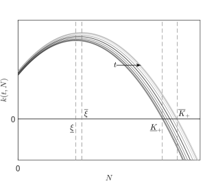
(a)

(b)

Figure 1: Qualitative shape of the function $k(t,N)$ in case of weak (a) and strong (b) Allee effect.

2.2 The functional response

The conditions on the functional response are the following:

(f1)

for all $t$, $f(t,0,P)\equiv 0$,

(f2)

for every $t,\;P$, $f(t,N,P)>0$ if $N>0$,

(f3)

for all $t$, fixed $N$, the function $P\mapsto f(t,N,P)$ is non-increasing in $P$ (or independent of it),

(f4)

for all $t$, fixed $P$, the function $N\mapsto f(t,N,P)$ is non-decreasing in $N$,

(f5)

for all $t$, there exists a non negative continuous function $f_{0}(t,P)$ such that it holds

$$f_{0}(t,P)=\lim_{N\to 0^{+}}\dfrac{f(t,N,P)}{N},$$

uniformly in $t\in\mathbb{R}$ and $P$ belonging to a compact set.

The first hypothesis imposes that predator functional response cannot be positive if there are no preys and the second implies that the functional response describes a loss term in the prey equation and a gain term in the predator one. The third one essentially says that the more the predators, the less one prey is expected to contribute to their growth; the fourth says that when there are more preys, each one contributes more to the growth of the predators. Finally, the fifth property is technical but reasonable; in particular it is used in the proof of Theorem 2.

Functional responses for predator–prey models widely used in literature satisfying these properties are listed in [garrione2016].

3 Persistence with a weak Allee effect

Assuming that the prey growth function describes a weak Allee effect (properties (gw1)–(gw4)), it is possible to obtain the following results, as in [garrione2016]. However, the proof of Theorem 1 differs from the one in [garrione2016], where the assumption on the monotonicity of $k$ with respect to $N$ is crucial.

Theorem 1.

Assume that the prey growth function satisfies the listed properties for a weak Allee effect (properties (gw1)–(gw4)). Consider the prey dynamics in absence of predator described by

$$\dot{N}=k(t,N)N-\nu N,$$ (3.1)

where $\nu>0$ is constant. Then, for every $0\leq\nu<\nu_{*}$ where

$$\nu*:=\dfrac{1}{T}\int_{0}^{T}k(s,0)ds,$$

equation (3.1) admits a unique, positive, bounded, globally asymptotically stable $T$-periodic solution $N^{*,\nu}$. Moreover,

$$\lim_{\nu\to 0}N^{*,\nu}(t)=N^{*,0}(t)\quad uniformly\;in\;t\in[0,T].$$ (3.2)

Proof.

Our proof follows [hale2012, p.128–129].

The trivial solution $N(t)\equiv 0$ is a $T$-periodic solution which, by the definition of $\nu$, is unstable. Hence there exists a positive solution $N(t)$ such that $\lim_{t\to+\infty}N(t)\neq 0$.

Moreover when $N>\overline{K}_{+}$ the right member of (3.1) is negative. Therefore $N(t)$ is bounded in $\mathbb{R}$ and approaches a $T$-periodic solution $N^{*,\nu}(t)$ as $t\to+\infty$. Furthermore, this $T$-periodic solution has the property $\underline{K}_{+}^{\nu}<N^{*,\nu}(t)<\overline{K}_{+}^{\nu}$ and hence is positive and bounded.

To prove the uniqueness of this $T$-periodic solution, we suppose that $N^{*,\nu}_{1}(t)$ and $N^{*,\nu}_{2}(t)$ are two $T$-periodic solutions such that $v(t):=N^{*,\nu}_{1}(t)-N^{*,\nu}_{2}(t)>0$ for all $t\in[0,T]$. (Note that this hypothesis is not restrictive; if there exists $\hat{t}$ such that $N^{*,\nu}_{1}(\hat{t})=N^{*,\nu}_{2}(\hat{t})=\hat{N}$, then $\hat{N}$ is an equilibrium point.)

Then we have

$$\dot{v}(t) =\dot{N}^{*,\nu}_{1}(t)-\dot{N}^{*,\nu}_{2}(t)$$

$$=\left(k(t,N^{*,\nu}_{1}(t))-\nu\right)N^{*,\nu}_{1}(t)-\left(k(t,N^{*,\nu}_{2}(t))-\nu\right)N^{*,\nu}_{2}(t)$$

$$=k(t,N^{*,\nu}_{1}(t))\left(N^{*,\nu}_{1}(t)-N^{*,\nu}_{2}(t)\right)+\left(k(t,N^{*,\nu}_{1}(t))-k(t,N^{*,\nu}_{2}(t))\right)N^{*,\nu}_{2}(t)+$$

$$-\nu\left(N^{*,\nu}_{1}(t)-N^{*,\nu}_{2}(t)\right).$$

Since $k(t,N)$ is decreasing in $[\xi(t),+\infty)$ with respect to $N$, we have that $k(t,N^{*,\nu}_{1}(t))-k(t,N^{*,\nu}_{2}(t))<0$, and then it turns out

$$\dot{v}(t)<k(t,N^{*,\nu}_{1}(t))v-\nu v.$$

Since we have

$$\dfrac{\dot{v}}{v}<k(t,N^{*,\nu}_{1}(t))-\nu,$$

we obtain

$$v(T)<v(0)\exp{\left(\int_{0}^{T}{\left(k(s,N^{*,\nu}_{1}(s))-\nu\right)ds}\right)}.$$

But remembering that $N^{*,\nu}_{1}(t)$ is a $T$-periodic orbit, we have

$$\int_{0}^{T}{\left(k(s,N^{*,\nu}_{1}(s))-\nu\right)ds}=\log{\dfrac{N^{*,\nu}_{1}(T)}{N^{*,\nu}_{1}(0)}}=0,$$

from which we obtain $v(T)<v(0)$ and the contradiction.

Finally, since $N^{*,\nu}(t)$ is the only $T$-periodic solution with positive initial data, it is globally asymptotically stable.

We have finally to prove the validity of (3.2). To this end, since the solutions $N^{*,\nu}$ satisfy (3.1) and they are bounded, thanks to the Gronwall’s lemma they are uniformly bounded with respect to $\nu$. Thus, denoting by $w_{\nu}$ the corresponding fixed point of $P^{T}_{\nu}$, the $T$-Poincaré operator associated with (3.1), we can assume without loss of generality that $w_{\nu}$ converges. In view of the uniqueness of the fixed point $w_{\nu}$ and the fact that $P^{T}_{\nu}$ depends continuously on $\nu$ when restricted to compact sets, we thus infer that $w_{\nu}\to w_{0}$, and the assertion (3.2) follows from the continuous dependence on the initial datum. ∎

Theorem 2.

Assume that the prey growth function and the functional response satisfy properties of a weak Allee effect (gw1)–(gw4) and (f1)–(f5), respectively. Then,

• the inequality

  $$\int_{0}^{T}{\left(\gamma(t)f(t,N^{*,0},0)-\delta_{1}(t)\right)dt}<0$$

  implies the extinction of predators for (2.1), i.e. $P(t)\to 0$ for $t\to+\infty$. Moreover we have $|N(t)-N^{*,0}(t)|\to 0$ for $t\to+\infty$.

• the inequality

  $$\int_{0}^{T}{\left(\gamma(t)f(t,N^{*,0},0)-\delta_{1}(t)\right)dt}>0$$

  implies the uniform persistence of both predators and prey for (2.1).

Proof.

Thanks to the previous result, the proof in [garrione2016, Proof of Theorem 3.2] holds also in this case without modifications. As invariant and absorbing set for system (2.1) we consider for a small $\varepsilon>0$

$${\cal K}^{\prime}=\left\{(N,P)\in\mathbb{R}^{2}_{+}:0\leq N\leq\overline{K}_{+}+\varepsilon,\;N+\dfrac{P}{\bar{\gamma}}\leq(\overline{K}_{+}+\varepsilon)\left(1+\dfrac{\overline{r}}{\underline{\delta}_{1}}\right)\right\},$$ (3.3)

with $\overline{r}:=\max_{t\in[0,T]}{k(t,\xi(t))}$. In fact, the axis are trajectories and we have that the vector field $F(t,N,P)=(F_{1}(t,N,P),F_{2}(t,N,P))$ associated to (2.1) satisfies:

$$F(t,N,P)_{|N=\overline{K}_{+}+\varepsilon}\cdot(1,0)=F_{1}(t,\overline{K}_{+}+\varepsilon,P)=k(t,\overline{K}_{+}+\varepsilon)(\overline{K}_{+}+\varepsilon)-f(t,\overline{K}_{+}+\varepsilon,P)P<0,$$

if $P>0,$ and, being for each $c\geq 0$

$$\dfrac{\hat{P}_{c}}{\bar{\gamma}}=(\overline{K}_{+}+\varepsilon)\left(1+\dfrac{\overline{r}}{\underline{\delta}_{1}}\right)-N+c,$$

$$\begin{array}[]{lll}F(t,N,\hat{P}_{c})\cdot\left(1,\dfrac{1}{\overline{\gamma}}\right)&\leq&\left(k(t,N)N-\dfrac{\delta_{1}}{\underline{\delta}_{1}}\overline{r}(\overline{K}_{+}+\varepsilon)\right)-\delta_{1}((\overline{K}_{+}+\varepsilon)-N+c)\\ &-&\hat{P}_{c}f(t,N,\hat{P}_{c})\left(1-\dfrac{\gamma}{\bar{\gamma}}\right)<0.\end{array}$$

As in [garrione2016] we obtain the existence of $\eta>0$ such that $\liminf_{t\to+\infty}P(t)>\eta$ if $N(0)\leavevmode\nobreak\ >\leavevmode\nobreak\ 0,$ $P(0)>0$. Now as in the mentioned paper easily follows the existence of $\delta>0$ such that $\limsup_{t\to+\infty}N(t)>\delta$ if $N(0)>0,\;P(0)>0$ and by [zhao2003, Theorem 1.3.3], we have that the system is uniformly persistent. ∎

Theorem 3.

Under the assumptions of Theorem 2, part (b), there exists a non-trivial $T$-periodic solution $(N(t),P(t))$ to (2.1) such that $N(t),\;P(t)>0$ for every $t\in[0,T]$.

Proof.

This result is a consequence of [zhao2003, Theorem 1.3.6], applied to the Poincaré map on the invariant set. ∎