E-mail: {pmediano, f.rosas}@imperial.ac.uk††thanks: P.M. and F.R. contributed equally to this work.
E-mail: {pmediano, f.rosas}@imperial.ac.uk
Beyond integrated information: A taxonomy of information dynamics phenomena
Abstract
Most information dynamics and statistical causal analysis frameworks rely on the common intuition that causal interactions are intrinsically pairwise – every ‘cause’ variable has an associated ‘effect’ variable, so that a ‘causal arrow’ can be drawn between them. However, analyses that depict interdependencies as directed graphs fail to discriminate the rich variety of modes of information flow that can coexist within a system. This, in turn, creates problems with attempts to operationalise the concepts of ‘dynamical complexity’ or ‘integrated information.’ To address this shortcoming, we combine concepts of partial information decomposition and integrated information, and obtain what we call Integrated Information Decomposition, or ID. We show how ID paves the way for more detailed analyses of interdependencies in multivariate time series, and sheds light on collective modes of information dynamics that have not been reported before. Additionally, ID reveals that what is typically referred to as ‘integration’ is actually an aggregate of several heterogeneous phenomena. Furthermore, ID can be used to formulate new, tailored measures of integrated information, as well as to understand and alleviate the limitations of existing measures.
How can we best characterise the plethora of dynamical phenomena that can emerge in a system of interdependent components? Progress on this question will enable important advances in our understanding, engineering and control of multivariate complex systems, including the human brain Kelso (1995), the global climate Runge et al. (2019), macroeconomics Dosi and Roventini (2019), and many more. A popular approach to study such systems is to portray their interdependencies as a directed graph of non-mediated dependencies from past to future events (for example with Granger causality Bressler and Seth (2011)); and then to analyse this graph. However, this approach has a serious limitation that is rarely acknowledged: it only considers statistical causation acting from single ‘cause’ variables to single ‘effect’ variables (or sets of variables), thus neglecting possible higher-order causal interactions.
The above limitation is rooted in the misleading intuition that information dynamics can be reduced to storage and transfer phenomena. Accordingly, a number of theoretical frameworks have tried to assess the dynamical complexity – understood as the amount of information transfer – of various systems using one-dimensional metrics. A remarkable example of this is found in the neuroscience literature, where it has been proposed that a key feature of the neural dynamics underpinning advanced cognition, flexible behaviour, and ultimately consciousness, can be captured by a single number that accounts for the ability of the system to ‘integrate information.’ There have been several operationalisations of this notion, including the various measures in Integrated Information Theory (IIT) Tononi et al. (1994); Balduzzi and Tononi (2008); Oizumi et al. (2014) and Causal Density (CD) Seth et al. (2011); however, these measures have been shown to behave inconsistently van Walsum et al. (2003); Mediano et al. (2019); Rosas et al. (2019), making empirical applications difficult to interpret. Other attempts to explain information dynamics solely in terms of storage and transfer have been shown to be similarly unsuccessful James et al. (2016).
As a possible way forward, Lizier Lizier (2010) postulated a third category, information modification, which informally appeals to the notion of ‘computation,’ although it still remains both theoretically and practically imprecisely defined. Following Lizier’s insight, we pursue a multi-dimensional description of dynamical complexity, which can disentangle qualitatively different modes of information dynamics and statistical causality. Our approach is based on the partial information decomposition (PID) framework Williams and Beer (2010), which breaks down the information that multiple source variables carry about a (single) target variable into redundant, unique and synergistic components. Applying PID to a stochastic dynamical system setting, we consider the decomposition of the whole set of ‘cause’- and ‘effect’-type informational relationships, and obtain what we call the Integrated Information Decomposition, ID. This new framework sheds light on modes of information dynamics that have not been previously reported, and which most statistical causation frameworks ignore. Additionally, ID allows us to show how existing one-dimensional measures of integrated information conflate qualitatively different phenomena.
Decomposing multivariate information
Consider two interdependent processes that are measured at regular time intervals. The excess entropy Crutchfield and Feldman (2003) of these processes, , is the total amount of (Shannon) information that is transferred through these processes from past to future, which is a well-known metric to assess dynamical complexity Grassberger (1986). While is in general hard to compute Crutchfield et al. (2009), for Markovian processes it simplifies to
| (1) |
where and denote the states at times and respectively, and the subscript denotes variable index. We consider the decomposition of into modes of information dynamics, focusing on systems with Markovian dynamics, leaving extensions to processes with memory for future work.
Forward and backward information decomposition
Our approach is to decompose using the principles of the Partial Information Decomposition (PID) framework Williams and Beer (2010). By focusing on how information flows from past to future, one can consider a forward PID that decomposes the information provided by and about the joint future as
Intuitively, corresponds to redundant information provided by both and about 111We use as a shorthand notation for the random vector .; (resp. ) refers to the unique information that only (resp. ) provides about ; and finally, accounts for the information that and provide about only when they are observed together, henceforth called synergistic information 222 was in fact proposed in Ref. Griffith (2014) as a measure of integrated information..
An equivalent decomposition can be built by considering the information that and contain about the past state . Correspondingly, a backward PID is given by
The forward and backward PID are related to the notions of cause (forward) and effect (backward) information in IIT. These two information decompositions provide complementary, but overlapping descriptions of the system’s dynamics. The next section explains how they can be unified in a single and encompassing description.
Integrated information decomposition: ID
This section develops the mathematical framework of our contribution. The goal is to provide a decomposition of similar to the two above, but that applies to both cause and effect information simultaneously. To do this, we solve PID’s limitation of having only one single target variable and move towards multi-target information decompositions.
Double-redundancy lattice
Let us begin by considering the redundancy lattice Williams and Beer (2010), which is used in PID to formalise our intuitive understanding of redundancy. Let be the collection given by
| (2) |
which are all the sets of subsets of where no element is contained in another 333In a general -variable case, is the set of antichains on the lattice , discussed in Williams and Beer (2010). We focus on the bivariate case for clarity, although our results hold for any ..
The elements of have a natural (partial) order relationship: for , one says that if for all there exists such that Williams and Beer (2010). The lattice that encodes the relationship is known as the redundancy lattice (Fig. 1), and guides the construction of the four terms in the PID.

Our first step is to build a product lattice over , in order to extend the notion of redundancy from PID to the case of multiple source and target variables (here , and , respectively). Extending Williams and Beer’s Williams and Beer (2010) notation, we denote sets of sources and targets using their indices only, with an arrow going from past to future. Hence, the nodes of the product lattice are denoted as for , and a partial ordering relationship among them is defined by
| (3) |
This relationship guarantees a lattice structure 444 A proof of this is provided in the Appendix. with 16 nodes, which is shown in Figure 2. An intuitive understanding of the product lattice is developed in the sections below.

Redundancies and atoms
The next ingredient in the PID recipe is a redundancy function, , that quantifies the ‘overlapping’ information about the target that is common to a set of sources Williams and Beer (2010). The redundancy function in PID includes the following terms: is the information about the target that is in either source, the information in source , and the information that is in both sources together. This subsection extends the notion of overlapping information to the multi-target setting.
For a given , the overlapping information that is common to sources and can be seen in targets is denoted as and referred to as the double-redundancy function. In the following, we assume that the double-redundancy function satisfies two axioms:
-
•
Axiom 1 (compatibility): if and with and non-empty subsets of , then the following cases can be reduced to the redundancy of PID or the mutual information 555We use the shorthand notation for .:
-
•
Axiom 2 (partial ordering): if then .
By exploiting these axioms, one can define ‘atoms’ that belong to each of the nodes via the Moebius inversion formula. Concretely, the integrated information atoms are defined as the quantities that guarantee the following condition for all :
| (4) |
In other words, corresponds to the information contained in node and not in any node below it in the lattice. These are analogues to the redundant, unique, and synergistic atoms in the forward and backward PID above, but using the product lattice as a scaffold. By inverting this relationship, one can find a recursive expression for calculating as
| (5) |
With all the tools at hand, we can deliver the promised decomposition of in terms of atoms of integrated information.
Definition 1.
The Integrated Information Decomposition (ID) of a system with Markovian dynamics is the collection of atoms defined from the redundancies via Eq. (5), which satisfy
| (6) |
It is direct to see that the ID of two time series gives 16 atoms that correspond to the lattice shown in Figure 2, which are computed from a linear transformation over the 16 redundancies. Interestingly, Axioms 1 and 2 allow us to compute all the terms once a single-target PID redundancy function has been chosen, with the sole exception of . All this is summarised in the following result.
Proposition 1.
Axioms 1 and 2 provide unique values for the 16 atoms of the product lattice (see Figure 2) after one defines (i) a single-target redundancy function , and (ii) an expression for .
In the same way as in PID the definition of gives 3 other terms (unique and synergy) as side-product, Proposition 1 shows that in the addition of the double-redundancy function gives 15 other terms for free 666Note that our framework does not prescribe a particular formula for . A discussion on this issue can be found in the supplementary material..
Throughout the rest of the article we outline how ID can be used to revise theories of information dynamics and integrated information, and how it can provide more detailed analyses of systems of interest.
Simple examples
To start developing our intuition about the ID atoms, let us decompose the mutual information between the present of one variable, , and its own future, , i.e. the information storage in variable Lizier (2010):
| (7) | ||||
Here, corresponds to redundant information in the sources that is present in both targets; is the redundant information in the sources that is eliminated from the -th source () and hence is only conserved in ; and similarly for the remaining atoms.
As another example, consider the transfer entropy from to (with ):
| (8) | ||||
As before, is the synergistic information present in the joint past that can be read through either or , and similarly for the rest of the terms.
In the following section we explore the possibilities offered by this decomposition, and its implications for causal analysis, IIT, and complex systems in general.
Results
Limitations of conventional causal discovery methods
Mutual information and transfer entropy (or linear variants of them, to which our conclusions also apply) are the building blocks of most popular methods of statistical causal discovery. We now show that these metrics have two kinds of limitations: they conflate multiple effects in counterintuitive ways, and they fail to capture some effects altogether.
First, let us focus on the decomposition of information storage in Eq. (7). Note that, although are not in this mutual information, shares the term with by virtue of them being considered part of the same multivariate stochastic process. Therefore, if one uses simple mutual information as a measure of storage one may include information that is not stored exclusively in a given variable, which may lead to paradoxical conclusions such as the sum of individual storages being greater than .
Next, consider the terms in the decomposition of transfer entropy in Eq. (8). Note that, of these, is the only ‘genuine’ transfer term – all others correspond to redundant or synergistic effects involving both variables in past or future. Furthermore, one of the ‘extra’ terms () is shared with , in a somewhat counterintuitive overlap between storage and transfer. Similar concerns have been discussed in the literature James et al. (2016), showing that transfer entropy per se cannot be taken as a pure measure of information transfer.
Finally, from the decompositions of the mutual information and conditional mutual information as shown above, it is clear that none of these quantities are able to capture the ID terms of the form . These terms correspond to ‘synergistic effects’ (i.e. causes whose effects only manifest on groups, rather than individual variables) and are neglected by standard causal discovery methods.
Information processing in complex systems
Based on ID, and building on Lizier’s work Lizier (2010), we propose an extended taxonomy of information dynamics, with 6 disjoint and qualitatively distinct phenomena:
- Storage
-
Information that remains in the same source set, even if it includes collective effects. Includes , , , and .
- Copy
-
Information that becomes duplicated. Includes , and .
- Transfer
-
Information that moves between variables. Includes , and .
- Erasure
-
Duplicated information that is pruned. Includes , and .
- Downward causation
-
Collective properties that define individual futures. Includes , , and .
- Upward causation
-
Collective properties that are defined by individuals. Includes , , and .
While downward causation has been discussed in the past James et al. (2016), upward causation and synergistic storage () have, to our knowledge, not been reported in the literature. This revised taxonomy leads to less ambiguous, and more quantifiable descriptions of information dynamics in complex systems, in addition to grounding abstract concepts such as upward and downward causation 777The relation between ID and causal emergence Seth (2010) will be described in a separate publication., and notions such as integrated information.
Different types of integration
One important conceptual result of our framework is that there are multiple qualitatively different ways in which a multivariate dynamical process can integrate information through combinations of redundant, unique, or synergistic effects. As elementary examples, consider the following systems of 2 binary variables:
-
•
A copy transfer system, in which are i.i.d. fair coin flips, and (i.e. one bit is shifted).
-
•
The downward XOR, in which are independent identically distributed fair coin flips, and .
-
•
The parity-preserving random (PPR), in which are i.i.d. fair coin flips, and (i.e. is a random string of the same parity as ).
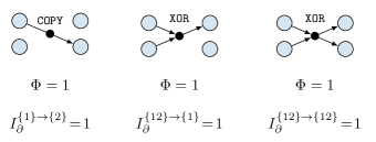
These three systems (Fig. 3) are ‘equally integrated,’ in the sense that the dynamics of the whole cannot be perfectly predicted from the parts alone and the integrated information measure (later defined in Eq. 9), yields for all of them Mediano et al. (2019); Barrett and Seth (2011). However, they integrate information in qualitatively different ways: in effect, the integration in the copy system is entirely due to transfer dynamics (); the downward XOR integrates information due to downward causation (); and PPR due to synergistic storage (). All the other ID atoms in each of these systems are zero (proofs in the Appendix).
Measures of integrated information
Within the IIT literature, researchers have proposed multiple measures aimed at quantifying to what extent the parts of a system affect each other’s temporal evolution. These measures, though superficially similar, are known to behave inconsistently, for reasons that are not always clear Mediano et al. (2019). Here we use ID to dissect and compare four existing measures of integrated information (, , ) and dynamical complexity (CD). We do not provide definitions of each measure here – for details see Section 2.2 of Ref. Mediano et al. (2019) and the original references Balduzzi and Tononi (2008); Griffith (2014); Oizumi et al. (2016).
As a systematic exploration, one can determine which measures are sensitive to which modes of information dynamics by calculating whether each measure is zero, positive, or negative for a system consisting of only one particular ID atom (Table 1; proofs in the Appendix). The main result is that each measure captures a different combination of ID atoms: although generally most of them capture synergistic effects and avoid (or penalise) redundant effects, they differ substantially. The key conclusion is that these measures are not simply different approximations of a unique concept of integration, but that they are capturing intrinsically different aspects of the system’s information dynamics. While aggregate measures like these can be empirically useful, one should keep in mind that they are measuring combinations of different effects within the system’s information dynamics. Echoing the conclusions of Ref. Mediano et al. (2019): these measures behave differently not only in practice, but also in principle.
| ID atoms | Measures | |||
|---|---|---|---|---|
| CD | ||||
| - | 0 | 0 | 0 | |
| 0 | 0 | 0 | 0 | |
| + | 0 | 0 | 0 | |
| 0 | + | 0 | + | |
| 0 | 0 | 0 | 0 | |
| + | + | 0 | + | |
| + | 0 | 0 | 0 | |
| + | + | + | + | |
| + | + | + | + | |
| + | 0 | + | 0 | |
Why whole-minus-sum can be negative
The ID can be further leveraged to provide elegant explanations of certain behaviours of integrated information and dynamical complexity measures. For example, , which is calculated as
| (9) |
for a bivariate process, can sometimes take negative values. This feature, which has been used as an argument to discard as a suitable measure of integrated information Griffith (2014); Oizumi et al. (2016), can be explained as follows. By applying the decomposition in Eq. (4), one finds that
Hence, accounts for all the synergies in the system (the seven terms in Fig. 2 with in either side), the unique information transferred between parts of the system, and, importantly, the negative of the bottom node of the ID lattice. The presence of this negative double-redundancy term shows that in highly redundant systems can be negative. This is akin to Williams and Beer’s Williams and Beer (2010) explanation of the negativity of the interaction information, applied to multivariate processes. Based on this insight, one can formulate a ‘corrected’ by adding back the double-redundancy:
which includes only synergistic and unique transfer terms.
We computed numerically for a simple example, using an extension of the PID presented by James et al. James et al. (2018). Mimicking the setting in Ref. Mediano et al. (2019) with discrete variables, let us consider a system in which are noisy AND gates of and the correlation between the noise components of and is a free parameter. We calculated and with respect to the system’s stationary distribution. Plots of the standard and corrected for this system are shown in Fig, 4, and details of the computation can be found in the Appendix.
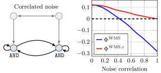
As expected, drops below zero as synergy decreases and redundancy increases with noise correlation. Interestingly, after adding the double-redundancy term, the corrected version, , tends to 0 for high noise correlation, which is more similar to some of the other measures highlighted in Mediano et al. (2019), e.g. CD and .
Why unnormalised causal density can exceed TDMI
999999footnotetext: Note that the original definition of causal density is normalised by , and has been proven to be bounded by mutual information Mediano et al. (2019).In Oizumi et al. Oizumi et al. (2016), the authors correctly point out that the sum of conditional pairwise transfer entropies (or unnormalised Causal Density; uCD) in a system can exceed the total mutual information, which is problematic for considering this as a measure of integrated information Oizumi et al. (2016); Note (999). This quantity, given by
| (10) |
can also be decomposed using ID. By applying Eq. (4) to the expression of uCD, one finds that
Besides the unique and synergistic terms that one would expect in a measure of information transfer Williams and Beer (2011), there is in addition a double-counting of a downward causation ID atom, . Specifically, uCD double-counts synergistic information in the past that is transferred redundantly to the future, and this can cause uCD to be greater than .
This finding makes it straightforward to design systems for which uCD is maximal (i.e. a system that has only ): are maximum entropy and . Indeed, for this system .
Discussion
We propose ID as a novel information-theoretic framework to study high-order interactions in time-series data. By unifying aspects of integrated information theory (IIT) and partial information decomposition (PID), the ID framework allows us to decompose information flow in a multivariate stochastic process into interpretable, disjoint parts. This allows systematic studies of unexplored modes of information dynamics – including modes of synergistic storage, and upward and downward causation – in a purely data-driven fashion.
Towards multi-dimensional measures of complexity
Besides the importance of having an encompassing taxonomy of information dynamics phenomena, this frameworks suggests, following Feldman and Crutchfield Feldman and Crutchfield (1998), that there is no theoretical basis to a purported all-encompassing scalar measure of dynamical complexity. The richness of complex dynamics is vast, and the prospect of subsuming all into a single number is unreasonable. Scalar measures might still have great practical value in certain contexts 888For example, measures that accurately discriminate between neural configurations corresponding to conscious and unconscious states in a particular experimental paradigm Casali et al. (2013).; nevertheless, a general theory of complex systems (biological or otherwise) cannot be reduced to a single, one-size-fits-all measure.
Integration measures conflate transfer and synergy
Using ID, one is able to inspect previous measures of integrated information, explaining similarities and differences between them, and fixing some of their shortcomings. Most importantly, we have shown that what is usually referred to as ‘integration’ is in fact an aggregate of several different information effects, typically including transfer and synergy phenomena. Moreover, different measures capture different effects in various proportions, which explains the heterogeneity among existing measures reported in Ref. Mediano et al. (2019). By employing ID one can tailor measures for targeting specific mixtures of effects, according to the information dynamics processes one wishes to analyse.
Causal analysis
998998footnotetext: Intuitively, a causal analysis reveals what the system could do, while a dynamical analysis based on attractor statistics reveals what the system actually does.As presented, ID is a generic tool to decompose multivariate mutual information, which can be directly used to perform causal analysis. Most integrated information measures can be roughly divided between those that describe integration in a system based on its causal properties Oizumi et al. (2014), and those that use the system’s attractor statistics, known as dynamical integration measures Mediano et al. (2019); Note (998). Given a system’s conditional probability distribution , one can use ID to perform either a causal or a dynamical analysis by using the stationary attractor distribution , or a maximum entropy distribution on . However, note that a few additional assumptions need to hold to interpret the results in a strict causal sense; in particular, the conditional distribution needs to be equivalent to a do() distribution in Pearl’s sense Pearl and Mackenzie (2018), and the system must satisfy the faithfulness and causal Markov conditions 999Also, note that the maximum entropy distributions employed by some causal integration frameworks are well-defined for discrete Markovian systems, but in general may not always exist Barrett and Mediano (2019)..
Limitations and future extensions
Our method inherits some of the limitations of PID. In particular, several distinct redundancy functions have been proposed for evaluating PID atoms, but there is not yet a consensus on one that is universally preferable James et al. (2018). Forthcoming work will explore how the framework yields new dynamical insights into redundancy function selection, and helps us address the current challenges of PID.
Acknowledgements.
The authors thank Julian Sutherland for valuable discussions. F.E.R. was supported by the Ad Astra Chandaria Foundation, and by the European Union’s H2020 research and innovation programme under the Marie Skłodowska-Curie grant agreement No. 702981. A.K.S. and A.B.B. acknowledge support from the Dr Mortimer and Theresa Sackler Foundation. A.K.S. also acknowledges support from the Canadian Institute for Advanced Research (CIFAR): Azrieli Programme on Brain, Mind, and Consciousness.Appendix A The product of two lattices is a lattice
A lattice is a partially ordered set for which every pair of elements has a well-defined meet and join , which correspond to their common greatest lower bound (infimum) and common least upper bound (supremum), respectively Charalambides (2002). Here we prove that, if is a lattice, then the product lattice equipped with the order relationship
| (11) |
is also a lattice, where . As a corollary of this, given that the set and partial ordering relationship used in PID are a lattice Williams and Beer (2010); Crampton and Loizou (2001), then the set and partial ordering relationship used in ID are also a lattice.
For compactness, let us use the notation and for . To prove the lattice structure of it suffices to show that
-
1.
is a valid meet; and
-
2.
is a valid join.
Note that the fact that is a lattice implies that and are well-defined for all .
Let us begin with the meet, for which we use as a shorthand notation. First, one can directly check that and , given the definition of above and the fact that (and similarly for , , and ). Next, we need to prove that for any such that and , we have (i.e. that is the greatest lower bound of and ). To see this, note that the conditions and imply the following four statements:
Using these relationships and the operator from , one can show that and , which in turn implies that . Finally, the proof for the join is analogous, replacing with and with .
Appendix B Decomposing PID atoms
Equation (4) in the main text shows how to decompose redundancies in the product lattice in terms of ID atoms. Here we provide a more general statement, that allows us to decompose not only redundancies, but also other PID atoms. The goal of this appendix is to build stronger connections between PID and , and to extend Proposition 1 to allow greater flexibility for specifying a function.
For the forward PID, and borrowing the notation from Williams and Beer Williams and Beer (2010), given a non-empty set of ‘future’ variables and an an element of the redundancy lattice , let us denote by the atom of the PID decomposition for , such that
| (12) |
We use an analogous notation for the backward PID, with a corresponding non-empty set of ‘past’ variables and , such that
| (13) |
Then, these quantities can be further decomposed in atoms as
| (14a) | |||
| (14b) | |||
Note that the sum runs only across one of the sets (instead of both as it does in Eq. (4) of the main text), and that every element in is also in , and hence the partial order relationship in the sums above is well-defined. As a few examples, in a bivariate system the following forward PID atoms decompose as:
These decompositions can be used to prove Proposition 1 of the main text. Adopting a view of ID as a linear system of equations, one needs 16 independent equations to solve for the 16 unknowns that are the atoms. Of those, 9 are given by standard Shannon mutual information (specifically, , , , and , for ) decomposed with Eq. (4) of the main text, and 6 are given by the single-target PIDs (, , and , as well as the 3 corresponding backward PIDs) decomposed by the expression above. Finally, one only need to add one individual atom to make the 16 equations needed, and the system can be solved for all other atoms.
Taking these results together, Proposition 1 in the main text can be generalised as follows: a valid ID can be defined not only in terms of redundancy, but also in terms of unique information or synergy. This is equivalent to the case of PID, for which decompositions based on unique information James et al. (2018) or synergy Quax et al. (2017); Rassouli et al. (2018) have been proposed. In fact, for the numerical results in Fig. 5 of the main text we use a ID based on unique information defined below.
Appendix C Computing the ID atoms
In Ref. James et al. (2018), James, Emenheiser and Crutchfield introduce a PID based on a new measure of unique information, , which we succinctly describe here. To define , they first define a constraint lattice on a set of variables (formally defined as the set of antichain covers with the natural partial ordering). Specifically, given a constraint and a probability distribution , consider the set of distributions that match marginals in with :
For example, the constraint determines the set of distributions such that and . In addition, the elements of (i.e. the nodes in the lattice) have an associated value of an information-theoretic measure evaluated on .
Let us focus on the bivariate PID: denote by the collection of edges of the constraint lattice for the variables , and let be the joint mutual information . For a link , one can evaluate the change in along the link via the operator ; e.g. . Additionally, for any let us define to be the set of all links that contain only at one side, i.e.
| (15) |
Then, the unique information is defined by
| (16) |
That is, the unique information is the smallest perturbation that is seen when adding the dependency between and . For further details, and a more pedagogical introduction, we refer the reader to the original paper James et al. (2018).
This measure can be naturally generalized to the ID setting by replacing above with the full joint mutual information and formulating the appropriate constraint lattice for . More precisely:
Definition 2.
Double-unique information based on dependencies. For a given set of variables , and two indices and , the double-unique information based on dependencies is defined as
| (17) |
This definition is applicable to both discrete and continuous random variables. In practice, the difficulty of calculating amounts to the difficulty of calculating maximum-entropy projections, which for Gaussian and discrete distributions is easily done with off-the-shelf software – in the case of discrete variables, for example using the dit package James et al. (2016). Once the double-unique information has been calculated, the same lattice can be reused to compute the unique information atoms for all 6 single-target PIDs, and together with the 9 MIs, these 16 numbers fully determine the numerical values of every ID atom.
It is important to recall that, as mentioned in the main body of the paper, the two axioms of ID do not uniquely determine . An exploration of alternative decompositions will be covered in a separate publication.
Appendix D Results of section ‘Different types of integration’
Here we present calculations for the example systems in Fig. 4 of the main text. These proofs hold for all ID that satisfy the partial ordering axiom of (Axiom 2 in the main text), have a non-negative double-redundancy function , and satisfy the following bound that follows from the basic properties of PID (c.f. Rosas et al. (2016)):
| (18) |
Let us examine the three systems in turn:
-
•
For the copy transfer system, , while and are independent i.i.d. fair coin flips. Since is independent from the rest of the system, , and due to partial ordering . Finally, using the Moebius inversion formula it follows that and all other atoms are zero.
-
•
In the downward XOR system, and are i.i.d. fair coin flips, , and is independent of the rest. Then, it is clear that , while . Additionally, note that , since . All this implies that all the redundancies (and hence all the atoms) below are zero, and hence due to the Moebius inversion formula.
-
•
Finally, consider the PPR system where are i.i.d. fair coin flips and is such that . Then . This implies that all redundancies (and hence atoms) except are zero, and hence using again the Moebius inversion formula .
Appendix E Results of section ‘Measures of integrated information’
In this appendix we prove the results in Table 1 of the main text, that shows whether each of four measures of integrated information (, CD, , ) are positive, negative, or zero in a system containing only one atom. A succinct definition of each measure is given below, and a comprehensive review and comparison of these and other measures can be found in Ref. Mediano et al. (2019).
Throughout this section we focus on bivariate systems, and use as variable indices, with . To complete the proof we will first show that it is possible to build systems with exactly one bit of information in one atom, and we will then compute the four measures on those systems.
Let us begin with the design of systems with one specific atom. Intuitively, this can be accomplished with a suitable combination of COPY and XOR gates for redundant and synergistic sets of variables, respectively. More formally, the procedure to build a system with and all other atoms equal to zero is as follows:
-
1.
Sample from a Bernoulli distribution with .
-
2.
Sample based on :
-
•
If , then .
-
•
If , then and is sampled from a Bernoulli distribution with .
-
•
If , then is a random string with parity .
-
•
-
3.
Sample based on analogously.
In all cases there will be one bit of information () shared between and , hence for any choice of . This can be proven using the fact that for any , one has , , and . To do so, let us start from the mutual information chain rule:
Rearranging the above terms, one can find that
where and . Finally, one finds that
which concludes the proof that . Furthermore, following a procedure similar to those in the previous section, it can be shown that any that satisfies the axioms described above (partial ordering, non-negative double-redundancy, and upper-bounded redundancy) correctly assigns 1 bit of information to , and 0 to all other atoms.
Now that we have built these 16 single-atom systems, let us move to the integration measures of interest. For CD, , and , we will proceed by decomposing them in terms of atoms and checking whether each atom is positive (+), negative (–), or absent (0) from the decomposition to obtain the results in Table 1 of the article. Let us begin with CD, defined as the sum of transfer entropies from one variable to the other:
| (19) | ||||
Similarly, for the atoms can be extracted from the decomposition of in Eq. (14a):
| (20) | ||||
For , the atoms can be extracted from the decomposition of Eq. (9) in the main text:
| (21) | ||||
The case is slightly more involved, since it is not easily decomposable into a sum of atoms. According to the definition of Oizumi et al. (2016), for a system given by the joint probability distribution one has
where is the manifold of probability distributions that satisfy the constraints
| (22) |
Therefore, it suffices to check whether the probability distribution of the system satisfies the constraints in Eq. (22) — if it does, then , and otherwise —, which can be easily verified for each system separately to obtain the column in Table 1, concluding the proof.
Appendix F Results of section ‘Why whole-minus-sum can be negative’
In this appendix we describe the details of the noisy AND system and how to compute its to yield the results shown in Figure 4 of the main text.
Given the past state of the system , the next state is given by
where are two auxiliary noise variables sampled from Bernoulli distributions with parameter , and they are sampled independently with probability and set to be identical to each other with probability . This results in a system that, for , consists of two separate AND gates with some noise, and for a system of two perfectly correlated components that at each time step change state with probability . All information-theoretic functionals are computed with respect to the system’s stationary distribution.
To compute the atoms we follow the procedure described above based on James et al.’s measure. To minimise numerical problems with the maximum-entropy projections involved, instead of computing all relevant quantities separately we compute one single constraint lattice for the whole system and read off all relevant quantities:
-
•
9 values of mutual information, which can be directly read from the corresponding nodes in the lattice;
-
•
6 values of single-target PID unique information, which can be obtained as the minimum of suitable subsets of the lattice according to Eq. (16); and
-
•
One double-unique information according to Eq. (17).
Together, these 16 numbers fully determine all 16 atoms, and the resulting linear system of equations can be easily solved.
References
- Kelso (1995) J. S. Kelso, Dynamic patterns: The self-organization of brain and behavior (MIT press, 1995).
- Runge et al. (2019) J. Runge, S. Bathiany, E. Bollt, G. Camps-Valls, D. Coumou, E. Deyle, C. Glymour, M. Kretschmer, M. D. Mahecha, J. Muñoz-Marí, et al., Nature Communications 10, 2553 (2019).
- Dosi and Roventini (2019) G. Dosi and A. Roventini, J Evol Econ 29 (2019).
- Bressler and Seth (2011) S. L. Bressler and A. K. Seth, Neuroimage 58, 323 (2011).
- Tononi et al. (1994) G. Tononi, O. Sporns, and G. Edelman, Proceedings of the National Academy of Sciences 91, 5033 (1994).
- Balduzzi and Tononi (2008) D. Balduzzi and G. Tononi, PLoS Computational Biology 4, 1 (2008).
- Oizumi et al. (2014) M. Oizumi, L. Albantakis, and G. Tononi, PLoS Computational Biology 10 (2014), 10.1371/journal.pcbi.1003588.
- Seth et al. (2011) A. K. Seth, A. B. Barrett, and L. Barnett, Philosophical Transactions of the Royal Society A: Mathematical, Physical and Engineering Sciences 369, 3748 (2011).
- van Walsum et al. (2003) A.-M. v. C. van Walsum, Y. Pijnenburg, H. Berendse, B. van Dijk, D. Knol, P. Scheltens, and C. Stam, Clinical Neurophysiology 114, 1034 (2003).
- Mediano et al. (2019) P. Mediano, A. Seth, and A. Barrett, Entropy 21, 17 (2019).
- Rosas et al. (2019) F. Rosas, P. A. M. Mediano, M. Gastpar, and H. J. Jensen, “Quantifying high-order interdependencies via multivariate extensions of the mutual information,” (2019), arXiv:1902.11239 [cs.IT] .
- James et al. (2016) R. G. James, N. Barnett, and J. P. Crutchfield, Physical Review Letters 116, 238701 (2016).
- Lizier (2010) J. Lizier, The local information dynamics of distributed computation in complex systems, Ph.D. thesis, University of Sydney (2010).
- Williams and Beer (2010) P. L. Williams and R. D. Beer, “Nonnegative decomposition of multivariate information,” (2010), arXiv:1004.2515 [cs.IT] .
- Crutchfield and Feldman (2003) J. P. Crutchfield and D. P. Feldman, Chaos: An Interdisciplinary Journal of Nonlinear Science 13, 25 (2003).
- Grassberger (1986) P. Grassberger, International Journal of Theoretical Physics 25, 907 (1986).
- Crutchfield et al. (2009) J. P. Crutchfield, C. J. Ellison, and J. R. Mahoney, Physical Review Letters 103, 094101 (2009).
- Note (1) We use as a shorthand notation for the random vector .
- Note (2) was in fact proposed in Ref. Griffith (2014) as a measure of integrated information.
- Note (3) In a general -variable case, is the set of antichains on the lattice , discussed in Williams and Beer (2010). We focus on the bivariate case for clarity, although our results hold for any .
- Note (4) A proof of this is provided in the Appendix.
- Note (5) We use the shorthand notation for .
- Note (6) Note that our framework does not prescribe a particular formula for . A discussion on this issue can be found in the supplementary material.
- Note (7) The relation between ID and causal emergence Seth (2010) will be described in a separate publication.
- Barrett and Seth (2011) A. B. Barrett and A. K. Seth, PLoS Computational Biology 7, 1 (2011).
- Griffith (2014) V. Griffith, “A principled infotheoretic -like measure,” (2014), arXiv:1401.0978 [cs.IT] .
- Oizumi et al. (2016) M. Oizumi, N. Tsuchiya, and S.-i. Amari, Proceedings of the National Academy of Sciences 113, 14817 (2016).
- James et al. (2018) R. G. James, J. Emenheiser, and J. P. Crutchfield, Journal of Physics A: Mathematical and Theoretical 52, 014002 (2018).
- Note (999) Note that the original definition of causal density is normalised by , and has been proven to be bounded by mutual information Mediano et al. (2019).
- Williams and Beer (2011) P. L. Williams and R. D. Beer, arXiv preprint arXiv:1102.1507 (2011).
- Feldman and Crutchfield (1998) D. P. Feldman and J. P. Crutchfield, Physics Letters A 238, 244 (1998).
- Note (8) For example, measures that accurately discriminate between neural configurations corresponding to conscious and unconscious states in a particular experimental paradigm Casali et al. (2013).
- Note (998) Intuitively, a causal analysis reveals what the system could do, while a dynamical analysis based on attractor statistics reveals what the system actually does.
- Pearl and Mackenzie (2018) J. Pearl and D. Mackenzie, The book of why: The new science of cause and effect (Basic Books, 2018).
- Note (9) Also, note that the maximum entropy distributions employed by some causal integration frameworks are well-defined for discrete Markovian systems, but in general may not always exist Barrett and Mediano (2019).
- Charalambides (2002) C. A. Charalambides, Enumerative combinatorics (Chapman and Hall/CRC, 2002).
- Crampton and Loizou (2001) J. Crampton and G. Loizou, International Mathematical Journal 1, 223 (2001).
- Quax et al. (2017) R. Quax, O. Har-Shemesh, and P. Sloot, Entropy 19, 85 (2017).
- Rassouli et al. (2018) B. Rassouli, F. Rosas, and D. Gündüz, in 2018 IEEE International Workshop on Information Forensics and Security (WIFS) (IEEE, 2018) pp. 1–7.
- Rosas et al. (2016) F. Rosas, V. Ntranos, C. Ellison, S. Pollin, and M. Verhelst, Entropy 18, 38 (2016).
- Seth (2010) A. K. Seth, Artificial life 16, 179 (2010).
- Casali et al. (2013) A. G. Casali, O. Gosseries, M. Rosanova, M. Boly, S. Sarasso, K. R. Casali, S. Casarotto, M.-A. Bruno, S. Laureys, G. Tononi, and M. Massimini, Science Translational Medicine 5, 198ra105 (2013).
- Barrett and Mediano (2019) A. Barrett and P. Mediano, Journal of Consciousness Studies 26, 11 (2019).