An Experiment on Network Density and
Sequential Learning

Abstract

We conduct a sequential social-learning experiment where subjects each guess a hidden state based on private signals and the guesses of a subset of their predecessors. A network determines the observable predecessors, and we compare subjects’ accuracy on sparse and dense networks. Accuracy gains from social learning are twice as large on sparse networks compared to dense networks. Models of naive inference where agents ignore correlation between observations predict this comparative static in network density, while the finding is difficult to reconcile with rational-learning models.

1 Introduction

In many economic situations, people form beliefs based on others’ actions. In these settings, agents typically do not observe all members of the society, but only a select subset — namely, their neighbors in an underlying social network. How the structure of this observation network affects learning outcomes is a fundamental question for understanding social learning. While an extensive theoretical literature has explored this question for both naive and rational agents (e.g., Golub and Jackson, 2010; Acemoglu, Dahleh, Lobel, and Ozdaglar, 2011; Golub and Jackson, 2012), much less is known empirically.

Density is one of the most basic properties of a network. How do learning patterns differ between sparse networks, where agents usually observe very few neighbors, and dense networks, where agents generally have abundant social information? On denser networks, agents observe more predecessors (both directly and indirectly), so their actions can incorporate the private signals of more individuals. But whether this leads to more accurate learning ultimately depends on how society aggregates these signals. Predecessors’ actions can be correlated by their common neighbors, so this aggregation may be difficult.

In this work, we conduct an experiment to compare social-learning outcomes on sparse and dense networks. We study a sequential social-learning environment where agents on an observation network each guess a hidden state. We find that although later agents have fewer observations on sparser networks, they nevertheless learn substantially better on sparse networks than dense networks.

We place subjects into groups of 40 who act in order. Each group lives on a social network, with randomly-generated links that determine each subject’s observations. Each subject has a 25% chance of observing each predecessor in the sparse treatment and a 75% chance in the dense treatment (and subjects know these probabilities). A hidden binary state is drawn for each group. On her turn, each subject must guess the state using her private signal and the past guesses of the predecessors she observes. Subjects were paid for accuracy.

Prior to data collection, we pre-registered a measure of long-run learning accuracy: the fraction of the final 8 subjects in the group who correctly guess the state. Comparing this measure on 130 sparse networks versus 130 dense networks, we find that denser networks lead to worse learning accuracy. In dense networks, the average accuracy of the last 8 subjects improves on the autarky benchmark (i.e., the average accuracy if no one can observe others’ actions) by 5.7%, but this improvement is 12.6% in sparse networks. Thus, the long-run accuracy gains from social learning are twice as large in the sparse treatment as in the dense treatment ($p$-value 0.0239).

In addition to its direct implications about the role of network density in social learning, this finding provides indirect evidence supporting models of naive inference in which agents neglect the correlations among their social observations (as in Eyster and Rabin, 2010). Motivated by a theoretical result from Dasaratha and He (2020), we compute predictions of the naive model. Later agents exhibit higher accuracy on sparse networks than dense networks in this model, as in our experimental evidence. The basic intuition is that an agent with correlation neglect ends up placing too much weight on the actions of the first few subjects in the same group, as these actions commonly influence many of the agent’s predecessors. When the network is denser, this over-weighting is more severe and so naive agents’ guesses are less accurate in the long run.

On the other hand, our experimental findings are inconsistent with the rational social-learning model. Acemoglu, Dahleh, Lobel, and Ozdaglar (2011)’s results imply that rational agents learn asymptotically in environments matching our experimental setup. We adapt their methods to provide lower bounds on the accuracy of rational agents 33 through 40 in the sparse and dense treatments. These bounds imply that rational agents’ accuracy cannot improve substantially from the dense-network treatment to the sparse-network treatment — in particular, the rational model does not predict a doubling of accuracy gain.

Our data also show that network density has no statistically significant effect on the overall accuracy averaged across all 40 subjects in each group. This is because dense networks increase the accuracy of subjects who move early in the group, even though they lower the accuracy of subjects who move later. This reversal of the accuracy ranking between sparse and dense networks over the course of social learning is another prediction of naive inference.

Finally, to provide additional evidence that learning is worse on denser networks because subjects fail to account for correlation, we conduct a variant of the experiment where subjects observe neighbors who make conditionally independent guesses. The setup is the same as in the main experiment, except the first $32$ agents in each group only observe their own private signals, while the final 8 agents randomly observe some of the initial $32$ agents. For the latter subjects, average guess accuracy is $68.2\%$ when there is a $25\%$ chance of observing each predecessor and $72.5\%$ when there is a $75\%$ chance of observing each predecessor. The extra observations in dense networks improve guess accuracy when those observations are not correlated by common social information.

1.1 Related Literature

Our experimental results add to a growing body of evidence that humans do not properly account for correlations in social-learning settings. Enke and Zimmermann (2017) show that correlation neglect is prevalent even in simple environments where the observed information sources are mechanically correlated. In a field experiment where agents interact repeatedly with the same set of neighbors, Chandrasekhar, Larreguy, and Xandri (2020) find agents fail to account for redundancies.

Most closely related to the present work, the laboratory games in Eyster, Rabin, and Weizsacker (2018) and Mueller-Frank and Neri (2015) directly evaluate behavioral assumptions matching ours. Eyster, Rabin, and Weizsacker (2018) find that on the complete observation network, many agents choose the best response assuming predecessors are rational while some participants exhibit redundancy neglect. On a more complex network the naive model matches more observations than the rational model, and there is little anti-imitation (which would be required for correct Bayesian inference, as shown in Eyster and Rabin, 2014). Mueller-Frank and Neri (2015) find most observations are consistent with the behavioral assumption we study (which they call quasi-Bayesian updating) in a setting where agents have limited information about the network. These experiments suggest naiveté may be more likely in settings where agents either have a limited knowledge of the true network or the network is known but very complicated. In these settings, the correct Bayesian belief given one’s observations can be far from obvious, so agents are more likely to resort to behavioral heuristics.

Unlike this previous work, our experiment tests the comparative statics predictions of naive and rational learning with respect to variations in the learning environment. This allows us to cleanly test redundancy neglect against rational updating. Our approach allows us to focus on long-term learning outcomes—which are the welfare-relevant metrics as we consider changes in the environment—instead of solely on measuring individual behavior.

Several experiments in this literature, including Grimm and Mengel (2018), Chandrasekhar, Larreguy, and Xandri (2020), and Mueller-Frank and Neri (2015), test social learning outcomes under multiple network structures. In these works, changes in network structure largely serve as a robustness check for claims about subject behavior. By considering larger networks and varying density, we show network structures play an important role in learning outcomes and exploit this variation to better understand behavior.

2 Theoretical Motivation

2.1 Model

The state of the world $\omega\in\{0,1\}$ takes one of two possible values with equal probabilities. The set of agents is indexed by $i\in\mathbf{\mathbb{N}}$. Agents move in the order of their indices, each acting once.

On her turn, each agent $i$ observes a private signal $s_{i}\in\mathbb{R}$, as well as the actions of some previous agents. Then, $i$ chooses an action $a_{i}\in\{0,1\}$ to maximize the probability that $a_{i}=\omega$ given her belief about $\omega$.

Private signals $(s_{i})$ are i.i.d. and Gaussian conditional on the state of the world. When $\omega=1$, $s_{i}\sim\mathcal{N}(1,\sigma^{2})$. When $\omega=0$, $s_{i}\sim\mathcal{N}(-1,\sigma^{2})$. Here $\sigma^{2}>0$ is the conditional variance of the private signal.

In addition to her signal, each agent $i$ observes the action of each predecessor with probability $q$. These observations are i.i.d. Independence of observations means that whether one agent observes a certain predecessor does not depend on whether a different agent observes the same predecessor. Agents observed by $i$ are called the neighbors of $i$, and the sets of neighbors define a (random) directed network.

We compare two kinds of agents: rational agents and naive agents. Rational agents play the unique perfect Bayesian equilibrium. Naive agents optimize given the following misspecified beliefs:

Assumption 1 (Naive Inference Assumption).

Each agent wrongly believes that each predecessor chooses an action to maximize her expected payoff based solely on her private signal, and not on her observation of other agents.

Equivalently, naive agents believe that each of their neighbors observe no other agents. Besides the error in Assumption 1, naive agents are otherwise correctly specified and optimize their expected utility given their mistaken beliefs.

Assumption 1 was introduced in a sequential-learning setting where agents observe all predecessors by Eyster and Rabin (2010). Their work refers to this form of inference as “best-response trailing naive inference” (BRTNI).

2.2 Naive and Rational Behavior

Dasaratha and He (2020) suggest an empirical test for the naive inference assumption: in the context of sequential learning on uniform random networks, does increasing the link-formation probability $q$ cause more inaccurate long-run beliefs? In this paper, we experimentally test this comparative static in networks of $40$ agents by comparing learning outcomes in sparse networks (where $q=\frac{1}{4}$) and dense networks (where $q=\frac{3}{4}$).

The naive-learning model and the rational-learning model make competing predictions about this comparative static. The intuition for naive learning comes from Dasaratha and He (2020), which suggests that overweighting due to correlation neglect is more severe on dense networks. We do not expect human subjects to behave exactly according to Assumption 1 — for example, the meta-analysis of Weizsäcker (2010) reports that laboratory subjects in sequential learning games suffer from autarky bias, underweighting their social observations relative to the payoff-maximizing strategy. However, the comparative static prediction of the naive model remains robust even after introducing any fraction of autarkic agents.

The prediction of the naive model is shown in Figure 1, which plots the probabilities that each of the 40 naive agents will correctly guess the state in sparse and dense networks with $\sigma=2.$ Because naive agents’ actions only depend on the number of their predecessors choosing each of the two actions and not the order of these actions, recursively calculating the distributions of actions is computationally feasible (see Appendix A.2 for details). As shown in Figure 1, early naive agents do worse under $q=\frac{1}{4}$ than $q=\frac{3}{4}$ because there is very little social information, but the comparison quickly reverses as we examine later naive agents.

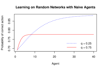
Figure 1: Learning accuracy on random networks with $40$ naive agents, binary actions, and $\sigma^{2}=4$. Dashed blue and solid red curves show the expected accuracy of different agents on networks with link probabilities $q=\frac{1}{4}$ and $q=\frac{3}{4}$, respectively.

On the other hand, the rational-learning model predicts that later agents will have either similar or greater accuracy on the dense network compared to the sparse network. Acemoglu, Dahleh, Lobel, and Ozdaglar (2011)’s results imply that in an environment matching our experimental setup, rational agents will learn the true state in the long-run, regardless of the network density. We can confirm that 40 rational agents are enough to approach this asymptotic learning limit when $q=\frac{3}{4}$. To do this, we compute a lower bound for the probability of correct learning for each agent $i$ in the dense network of our experiment, assuming all agents are rational Bayesians (see Appendix A.1 for details). This lower bound is based on (suboptimal) agent strategies that only depend on own private signals and the action of just one neighbor, as in the neighbor-choice functions in Lobel and Sadler (2015). This exercise shows that the $33^{\text{rd}}$ rational agent is correct at least 96.8% of the time on dense networks, with the lower bound on accuracy continuing to increase up to the $40^{\text{th}}$ agent, who is correct at least $97.5\%$ of the time. In addition to suggesting that the asymptotic result of Acemoglu, Dahleh, Lobel, and Ozdaglar (2011) very likely holds by the $40^{\text{th}}$ agent, the fact that this lower bound for accuracy on the dense network is so close to perfect learning proves the $40^{\text{th}}$ rational agent could not perform substantially better on the sparse network, contrary to the predicted improvement for the $40^{\text{th}}$ naive agent shown in Figure 1.

Intuitively one might also expect more connections to also help rational agents in the short- and medium-run as they can adjust for potential redundancies in information. For example, on the complete network with continuous actions, rational agents can back out the private signals of all predecessors by observing their actions, so every agent $i$ does better on the complete network than on any sparser network structure. We note, however, that exact comparative statics of the rational model or variants are not known on random networks.

We experimentally test the competing predictions of the naive and the rational models about how long-run accuracy varies with network density. We thus provide indirect evidence for the naive inference assumption, complementing the direct measurement of behavior in Eyster, Rabin, and Weizsacker (2018) and Mueller-Frank and Neri (2015).

Beyond providing another form of evidence, our experiment also contributes to understanding social learning by using the welfare-relevant outcome, namely the long-run accuracy of actions, as the dependent variable. Even if individual behavior tends to match redundancy neglect models in simple or stylized settings, one might worry that the theoretical implications of said models concerning aggregate learning need not hold in practice for complex environments. For a policymaker who can alter the observation network, for instance, experiments using welfare-relevant outcomes as their dependent variables give more explicit guidance as to the consequences of different policies.

3 Experimental Design

We conducted our experiment on the online labor platform Amazon Mechanical Turk (MTurk) using Qualtrics survey software.

We pre-registered our experimental protocol and regression specification prior to the start of the experiment in August 2017. Our pre-registration included the target sample size (which was met exactly) and the dependent variable to measure the accuracy of social learning. The pre-registration document can be found on the registry website at https://aspredicted.org/yp6eq.pdf and is also included in the Online Appendix.

We recruited $1040$ subjects. To be recruited, each subject must correctly answer three comprehension questions (which were scenarios in the game with a dominant choice). An additional $375$ MTurk users incorrectly answered one or more comprehension questions and were not allowed to participate in the experiment, based on the pre-registered exclusion criteria. These excluded users were $26.5\%$ of the potential subjects. The experiment was carried out in fall 2017.

In addition to comprehension questions, we restricted to subjects located in the United States who had completed at least $50$ previous MTurk tasks with a lifetime approval rate of at least $90\%$. Subjects were not permitted to participate multiple times in the experiment. There were at most $15$ subjects who did not complete all trials, implying a completion rate of at least $98.5\%$. These non-completers were excluded and replaced by new subjects.

Each trial consisted of 40 agents who were asked to each make a binary guess between two a priori equally likely states of the world, L (for left) and R (for right). The states were color-coded to make instructions and observations more reader-friendly. Agents are assigned positions in the sequence and move in order. Each MTurk subject participated in 10 trials, all in the same position (depending on when they participated in the experiment). The grouping of subjects into trials was independent across trials. Subjects received $\$0.25$ for completing the experiment and $\$0.25$ per correct guess, for a maximum possible payment of $\$2.75$. Subjects received no feedback about the accuracy of their guesses until they were paid at the conclusion of the experiment. Subjects ordinarily took less than $10$ minutes to complete their participation and earned $2.08 on average, so the incentives were quite large for an MTurk task.

In each trial, every agent received a private signal, which had the Gaussian distribution $\mathcal{N}(-1,4)$ in state L and the Gaussian distribution $\mathcal{N}(1,4)$ in state R. These distributions were presented visually in the instructions. Along with the value of their signal, subjects were told the probability of each state conditional on only their private signal.

Each trial was also associated with a density parameter, either $q=\frac{1}{4}$ or $q=\frac{3}{4}.$ A random network was generated for each trial by linking each agent with each predecessor with probability $q$. Each MTurk subject was assigned into either the “sparse” or the “dense” treatment, and then placed into 10 trials either all with $q=\frac{1}{4}$ or all with $q=\frac{3}{4}.$ So there were 520 subjects and 130 trials for each treatment. Agents were told the actions of each linked predecessor and the link probability $q$ (but not the full realized network, which could not be presented succinctly).

In each trial, agents viewed their private signal and any social observations and were asked to guess the state. States, signals, and networks were independently drawn across trials. Experimental instructions and an example of a choice screen are shown in the Online Appendix.

4 Results

Let $y_{i,j}$ be the indicator random variable with $y_{i,j}=1$ if agent $i$ in trial $j$ correctly guesses the state, $y_{i,j}=0$ otherwise. Define $\tilde{y}_{j}:=\frac{1}{8}\sum_{i=33}^{40}y_{i,j}$ as the fraction of the last 8 agents in trial $j$ who correctly guess the state. We test learning outcomes for the final 8 agents because welfare depends on long-run learning outcomes in large societies and these agents better approximate long-run outcomes. By using only her private signal, an agent can correctly guess the state 69.15% of the time. We call $\tilde{y}_{j}-0.6915$ the gain from social learning in trial $j$, as this quantity represents improvement relative to the autarky benchmark.

We find that the average gain from social learning is 8.73 percentage points for the $q=\frac{1}{4}$ treatment and 4.12 percentage points for the $q=\frac{3}{4}$ treatment. Social learning improves accuracy on the sparse networks by twice as much as on the dense networks. To test for statistical significance, we consider the regression

$$\tilde{y}_{j}=\beta_{0}+\beta_{1}q_{j}+\epsilon_{j}$$

where $q_{j}\in\{\frac{1}{4},\frac{3}{4}\}$ is the network density parameter for trial $j$. Recall that each subject was assigned into ten random trials with the same network density and in the same sequential position. This means for two different trials $j^{{}^{\prime}}\neq j^{{}^{\prime\prime}}$, the error terms $\epsilon_{j^{{}^{\prime}}}$ and $\epsilon_{j^{{}^{\prime\prime}}}$ are close to independent since there are likely very few subjects who participated in both trials.

We estimate $\beta_{1}=-0.092$ with a $p$-value of 0.0239 (see Table 1). The results are the same whether we use robust standard errors or not. These findings are consistent with naive updating but not with rational updating, as discussed in Section 2.

	FractionCorrect
NetworkDensity	-0.0923
	(0.0406)
Constant	0.802
	(0.0218)
Observations	260
Adjusted $R^{2}$	0.016

Table 1: Regression results for the effect of network density on learning outcomes (with robust standard errors).

This difference in the gains from social learning is not driven by different rates of autarky among the two treatments for the last 8 agents. We say an agent goes against her signal if she guesses L when her signal is positive or guesses R when her signal is negative. Within the last 8 rounds, there are 138 instances of agents going against their signals in the $q=\frac{1}{4}$ treatment, which is very close to the 136 instances of the same under the $q=\frac{3}{4}$ treatment. However, when agents go against their signals in the last 8 rounds, they correctly guess the state 81.88% of the time under the $q=\frac{1}{4}$ treatment, but only 71.32% of the time under the $q=\frac{3}{4}$ treatment. This shows the observed difference in accuracy is due to social learning being differentially effective on the two network structures.

However, the $q=\frac{3}{4}$ treatment yields better learning outcomes for early agents. For agents 10 through 20, the average guess accuracy is 72.24% under the $q=\frac{1}{4}$ treatment and 73.22% under the $q=\frac{3}{4}$ treatment. As such, if we replace the dependent variable in the pre-registered regression with overall accuracy $\bar{y}_{j}:=\frac{1}{40}\sum_{i=1}^{40}y_{i,j}$, then we do not find a statistically significant estimate for $\beta_{1}$ ($p$-value of 0.663). This result is consistent with the naive-learning model: according to the predictions of the naive model shown in Figure 1, early agents are more accurate under $q=\frac{3}{4}$, but later agents are more accurate under $q=\frac{1}{4}.$ The point of overtaking happens at a later round in practice than in theory, because our experimental subjects rely more on their private signal than predicted by the naive model, consistent with the meta-analysis of Weizsäcker (2010).

Our experiment was designed to compare long-run learning accuracy on different networks instead of measuring individual behavior. We do not directly test alternate behavioral models for two reasons. First, given the complex signal and network structures, such tests will be very noisy in our data. Second, because the spaces of possible networks and actions have very high dimension, it is computationally infeasible to determine the action that each agent would take under common knowledge of rationality. However, in the next subsection we provide some evidence that our findings are driven by herding under naive inference rather than other behavioral mechanisms.

4.1 Evidence of naive herding

In this section, we present three pieces of evidence suggesting that naive herding is the mechanism responsible for the difference in learning accuracy between the two treatments.

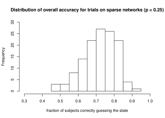
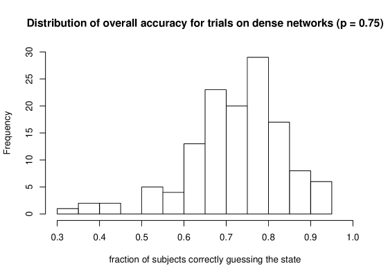
Figure 2: Histograms of fractions of agents correctly guessing the state

(1) Distribution of overall accuracy. Figure 2 in Appendix B plots the distributions of subjects who correctly guess the state in the $q=\frac{1}{4}$ and $q=\frac{3}{4}$ treatments, across different trials. Compared to the distribution under $q=\frac{1}{4}$, the distribution under $q=\frac{3}{4}$ has more extreme values and a larger standard deviation (11.36 percentage points versus 9.12 percentage points). This is suggestive evidence for naive herding. With denser networks, we simultaneously find more trials where agents do very badly overall (from herding on the wrong state) and more trials where agents do very well overall (from herding on the correct state).

(2) Effect of misleading early signals on the accuracy of later agents. Call a private signal misleading if it is positive while the state is L, or if it is negative while the state is R. If naive herding is the mechanism, we would expect misleading signals received by early agents to be more harmful for eventual learning accuracy on denser networks than on sparser networks. On the other hand, a different behavioral mechanism based on the salience of the visible decisions would suggest that early misleading signals are more harmful on sparse networks, since each visible decision is more salient when agents have fewer social observations. To test the naive herding mechanism, we expand our baseline regression to include two additional regressors: the number $m_{j}$ of the first fifth of agents who receive misleading signals in trial $j$, and its interaction effect with network density. That is, we estimate

$$\tilde{y}_{j}=\beta_{0}+\beta_{1}q_{j}+\beta_{2}m_{j}+\gamma(q_{j}m_{j})+\epsilon_{j}.$$

The difference in the marginal effect of a misleading early signal for learning accuracy on the dense network $(q=\frac{3}{4})$ versus on the sparse network $(q=\frac{1}{4})$ is $\frac{1}{2}\gamma$ in the above specification.

As reported in Table 5 in Appendix B, we find $\gamma=0.05$ with a $p$-value of 0.0923. This means each misleading signal among the first fifth of agents harms the average accuracy of the last fifth of agents in the same trial by an extra 2.5 percentage points in dense networks compared to sparse networks.

(3) Average uncertainty. Based on simulation evidence, we expect naive agents to exhibit more agreement on denser networks. To test this prediction in the data, we consider for each trial a set of 30 moving windows centered around periods 6, 7, … 35, with each window spanning 11 consecutive periods. For each trial $j$ and each window $w$, we compute $r_{j,w}\in\{0,\frac{1}{11},...,1\}$ as the fraction of 11 agents in the window who guessed R, and we let $u_{j,w}:=r_{j,w}\cdot(1-r_{j,w})$ be a measure of uncertainty within the window. In windows where agents exhibit a greater degree of agreement, we will see a lower $u_{j,w}$. Under herding, we expect lower uncertainty on denser networks, as higher density accelerates convergence to a (possibly mistaken) social consensus. We find in the data that the average uncertainty across all trials and all windows is 0.165 on dense networks and 0.178 on sparse networks. Examining uncertainty in each of the 30 windows $w$ separately, we find average $u_{j,w}$ across trials is lower among dense networks than sparse networks for all but 1 out of 30 windows. Numerically, the naive herding theory predicts lower average $u_{j,w}$ on denser networks in all 30 windows.

5 Neighbors with Conditionally Independent Actions

In our main experiment, we find that denser networks lead to worse social learning by later subjects. We have presented evidence suggesting the mechanism behind this result is that subjects neglect correlation in observed actions. To provide additional evidence for this channel, we now test how network density affects social learning when observed actions are conditionally independent given the state. In this section, we will ask whether more observations help subjects whose neighbors only have private information.

5.1 Experimental Design

We also pre-registered the experimental protocol and regression specification for this second experiment, including the dependent variable to measure the accuracy of social learning and the target sample size, prior to the start of the experiment in November 2020. The pre-registration document is included in the Online Appendix and may also be accessed via the registry website at https://aspredicted.org/ag8fr.pdf.

This experiment was also conducted online on MTurk. We recruited $624$ subjects, and each subject participated in $10$ trials. There were a total of $130$ trials. To increase power, each trial included subjects in both sparse and dense treatments. The first $32$ subjects in each trial had no neighbors, and chose actions based only on their private signals. Each trial also contained $8$ subjects in the sparse treatment and $8$ subjects in the dense treatment. Subjects in the sparse treatment observed each of the first $32$ subjects in the same trial with probability $q=\frac{1}{4}$ while subjects in the dense treatment observed each of the first $32$ subjects with probability $q=\frac{3}{4}$. There were no other observations, so the actions of the observed neighbors are always uncorrelated given the state. In particular, the subjects after the first 32 in each trial never observe each other.

We maintained the state distribution, private signal distribution, and action space from the main experiment. Recruitment and payment were also the same as in the main experiment. The experimental instructions were modified to accurately describe the social information subjects would receive, if any. The first $32$ subjects in each trial (like the first subject in each trial in the main experiment) were only asked the one comprehension question that just involves private signals, as the other comprehension questions pertain to subjects who receive social information. Subjects earned an average of $1.90 per person in this second experiment.

5.2 Results

We find that the average accuracy is $68.2\%$ in the sparse treatment and $72.5\%$ in the dense treatment. When subjects’ neighbors only have private information and not social information, having more neighbors improves the accuracy of guesses.

In each trial, we will index the $8$ subjects in the sparse treatment as $33,\ldots,40$ and the $8$ subjects in the dense treatment as $41,\ldots,48$. Let $y_{i,j}$ be the indicator random variable with $y_{i,j}=1$ if agent $i$ in trial $j$ correctly guesses the state, $y_{i,j}=0$ otherwise. For each $q\in\left\{\frac{1}{4},\frac{3}{4}\right\}$, we define $\tilde{y}_{j}^{q}$ as the fraction of the 8 subjects in that treatment in trial $j$ who correctly guess the state, so

$$\tilde{y}_{j}^{\frac{1}{4}}:=\frac{1}{8}\sum_{i=33}^{40}y_{i,j}\text{ and $\tilde{y}_{j}^{\frac{3}{4}}$:=$\frac{1}{8}\sum_{i=41}^{48}y_{i,j}$}.$$

To test for statistical significance, we consider the regression

$$\tilde{y}_{j}^{q}=\beta_{0}^{uncor}+\beta_{1}^{uncor}q+\epsilon_{j,q}$$

where $q\in\{\frac{1}{4},\frac{3}{4}\}$ is the network density parameter. We estimate $\beta_{1}^{uncor}=0.087$ with a $p$-value of $0.0391$ (see Table 2).

	FractionCorrect
NetworkDensity	0.0865
	(0.0417)
Constant	0.660
	( 0.0229)
Observations	260
Adjusted $R^{2}$	0.013

Table 2: Regression results for the effect of network density on learning outcomes for subjects observing neighbors with only private information (with robust standard errors).

The difference in average accuracy is again driven by a difference in the value of social information. Recall that a subject goes against her signal if her signal is positive and she chooses L or her signal is negative and she chooses R. Conditional on going against one’s own signal, subjects correctly guess the state $53.66\%$ of the time in sparse treatment and $69.39\%$ of the time in dense treatment.

Guesses are in general less accurate in this follow-up experiment than in the main experiment. The subjects in the first $32$ positions in each trial had only one comprehension question because their decision problems did not involve any social information. Subjects who did not fully understand the experimental instructions may therefore have been more likely to participate in the experiment in these positions, producing much noisier choices that degrade later subjects’ accuracy. There may also be differences in the MTurk subject pool compared to the main experiment, as the second experiment was conducted three years later.

The follow-up experiment finds that having more observations improves accuracy when those observations are conditionally uncorrelated. This provides additional evidence that our main result is driven by the failure of subjects to account for correlation in observed actions, rather than by some other mechanism that does not depend on this correlation.

6 Concluding Discussion

Our study provides experimental evidence on how the density of the observation network affects people’s long-run accuracy in social-learning settings. We find that sparser networks double the accuracy gains from social learning relative to denser networks. While the rational model predicts correct asymptotic social learning with minimal assumptions on the social network, we conjecture that in practice, many structural properties of the network can substantially alter long-run accuracy. Our empirical findings support this conjecture for the case of network density, one of the most canonical network statistics. We leave open the roles of other network structures as promising future work.

We have argued that our experimental results provide evidence for inferential naiveté by analyzing a particular form of behavior (Assumption 1). We conclude by discussing two ways in which the experimental results are potentially consistent with more general models of behavior. First, we have discussed models where all agents are rational or all agents are naive, but a model where only some of the agents suffer from inferential naiveté may be more realistic. Such a model could also generate herding on incorrect beliefs, and this herding may be more likely on denser networks. The exact details depend on how the agents who do not suffer from inferential naiveté reason about others’ play. If these agents wrongly believe that others are playing the perfect Bayesian equilibrium strategies, then they will fail to correct the mistakes of naive agents. In this case, early agents’ actions can have very disproportionate influence on later agents.

Second, Assumption 1 is a particular form of naive updating that assumes agents entirely neglect correlations in neighbors’ actions. Even in homogeneous populations, intermediate forms of naive updating could also generate herding on incorrect beliefs. Our main result suggests inferential naiveté, but does not distinguish between alternate naive models involving some correlation neglect.

Appendix

Appendix A Theoretical Predictions in the Experimental Environment

A.1 Bounding the Performance of Rational Agents

Consider 40 rational agents on a random network where each agent is linked to each of her predecessors $\frac{3}{4}$ of the time, i.i.d. across link realizations. Agents know their own neighbors but have no further knowledge about the realization of the random network. The signal structure and payoff structure match the experimental design in Section 3.

We provide a lower bound for the accuracy of agents 33 through 40 in the unique PBE of the social-learning game. We first show that when every player uses the equilibrium strategy, all agents learn at least as well as when everyone uses any constrained strategy that chooses an action based on only own private signal and the action of the most recent neighbor. We then exhibit payoffs under one such strategy, which give a lower bound on rational performance.

Fix an arbitrary sequence of constrained strategies $(\sigma_{i})$ where $\sigma_{i}:S_{i}\times\{0,1,\emptyset\}\to\Delta(\{0,1\})$ is only a function of $i$’s signal $s_{i}$ and the action of the most recent predecessor that $i$ observes ($\sigma_{i}(s_{i},\emptyset)$ refers to $i$’s play if $i$ does not observe any predecessor). Let $a_{i}$ denote $i$’s (random) action induced by this sequence of strategies. Let $a^{\prime}_{i}$ denote $i$’s (random) action when all agents use the PBE strategy.

Claim 1.

For all $i$, $\mathbb{P}[a^{\prime}_{i}=\omega]\mathbb{\geq P}[a_{i}=\omega].$

Proof.

The proof is by induction on $i$ and the base case of $i=1$ is clear. Suppose the claim holds for $i=1,...,n$. Conditional on agent $n+1$ observing no predecessors, the claim again holds as in the base case, so we can check the claim conditional on $n+1$ observing at least one neighbor.

Let $j$ be the most recent neighbor that $n+1$ observes. Then the rational agent observes $s_{n+1}$, $a^{\prime}_{j}$ for some $j\leq n$, and perhaps some other actions while the constrained agent only uses $s_{n+1}$ and $a_{j}$ in decision-making, where $\mathbb{P}[a^{\prime}_{j}=\omega]\mathbb{\geq P}[a_{j}=\omega]$ by the inductive hypothesis. By garbling the observed action $a^{\prime}_{j}$, the rational agent could construct a random variable with the same joint distribution with $\omega$ as the less accurate action $a_{j}$. Ignoring information other than $s_{n+1}$ and the garbled $a^{\prime}_{j},$ the rational agent $n+1$ could therefore follow a strategy that does as well as agent $n+1$ under the strategy profile $(\sigma_{i})$. So we must have $\mathbb{P}[a^{\prime}_{n+1}=\omega]\mathbb{\geq P}[a_{n+1}=\omega]$ when everyone uses the PBE strategy. ∎

We then numerically compute the values for $\mathbb{P}[a_{{}_{i}}=\omega]$ under the optimal constrained strategy, which are displayed in Table 3.

agent number

probability correct

33	34	35	36	37	38	39	40
0.9685	0.9695	0.9705	0.9714	0.9723	0.9731	0.9739	0.9746

Table 3: Lower bounds on the accuracy of rational agents on dense networks.

A.2 Performance of Naive Agents

Consider $40$ naive agents on a random network where each agent is linked to each of her predecessors with probability $q$, i.i.d. across link realizations. The signal structure and payoff structure match the experimental design in Section 3.

We will compute the accuracy of each agent by a recursive calculation. Because naive agents’ actions do not depend on the order of predecessors, behavior depends only on the number of agents who have played L and the number of agents who have played R as well as the network. We will compute the distribution over the number of agents from the first $n$ who have played L and the number who have played R recursively.

Assume the state is R. Let $P(k,k^{\prime})$ be the probability that $k$ of the first $n$ agents play L and $k^{\prime}$ of the first $n$ agents play R. We define $P(k,k^{\prime})=0$ if $k<0$ or $k^{\prime}<0.$ The posterior log-likelihood of state R for a naive agent observing one action equal to R (and no signal) is

$$\ell=\frac{2}{\sigma^{2}}\cdot\frac{\mu+\sigma\phi(-\mu/\sigma)}{1-\Phi(-\mu/\sigma)},$$

where $\Phi$ and $\phi$ are the distribution function and probability density function of a standard Gaussian random variable, respectively.

Then we have the recursive relation

$$P(k,k^{\prime}) =P(k-1,k^{\prime})\sum_{i\leq k-1,i^{\prime}\leq k^{\prime}}B(i,k-1,q)B(i^{\prime},k^{\prime},q)\Phi(\frac{\sigma(i-i^{\prime})\ell-2\mu\sigma}{2})+$$

$$P(k,k^{\prime}-1)\sum_{i\leq k,i^{\prime}\leq k^{\prime}-1}B(i,k,q)B(i^{\prime},k^{\prime}-1,q)[1-\Phi(\frac{\sigma(i-i^{\prime})\ell-2\mu\sigma}{2})],$$

where $B(i,k,q)$ is the probability a binomial distribution with parameters $k$ and $q$ is equal to $i$. The first summand gives the probability of agent $k+k^{\prime}$ choosing L after $k-1$ predecessors choose L and the remainder choose R, and the second summand gives the probability of agent $k+k^{\prime}$ choosing R after $k$ predecessors choose L and the remainder choose R. The binomial coefficients correspond to the possible network realizations. Here we use naive inference, which implies that only the number of observed agents choosing each action matters for behavior and not their order.

From these distributions $P(\cdot,\cdot)$ we can compute the probability that agent $n$ chooses the correct action R:

$$\sum_{k=0}^{n}P(k,n-k)\sum_{i\leq k,i^{\prime}\leq n-k}B(i,k,q)B(i^{\prime},n-k,q)[1-\Phi(\frac{\sigma(i-i^{\prime})\ell-2\mu\sigma}{2})].$$

These probabilities, which we compute numerically, are displayed in Table 4 for agents $33$ through $40$.

agent number
accuracy with $q=1/4$
accuracy with $q=3/4$

33	34	35	36	37	38	39	40
0.8773	0.8780	0.8786	0.8792	0.8797	0.8801	0.8805	0.8808
0.7768	0.7768	0.7768	0.7768	0.7768	0.7768	0.7768	0.7768

Table 4: The accuracy of naive agents on sparse and dense networks.

Appendix B Relegated Figures and Tables

	Dependent variable:
	FractionCorrect
MisleadingEarlySignals	0.014
	(0.017)
NetworkDensity	0.033
	(0.082)
MisleadingEarlySignals$\times$NetworkDensity	$-$0.050∗
	(0.030)
Constant	0.768∗∗∗
	(0.045)
Observations	260
R2	0.040
Adjusted R2	0.029
Residual Std. Error	0.163 (df = 256)
F Statistic	3.566∗∗ (df = 3; 256)
Note:	∗p$<$0.1; ∗∗p$<$0.05; ∗∗∗p$<$0.01

Table 5: Effect of misleading early signals.

Online Appendix

Appendix C Experimental Instructions

Instructions and an example choice follow. To avoid confusion, the instructions were modified for player $1$ in each round to exclude discussion of social observations. A sample experiment can be completed online at https://upenn.co1.qualtrics.com/jfe/form/SV_42dq2J2wHO30zA1

Appendix D Pre-Registration Documents

References

- Acemoglu et al. (2011) Acemoglu, D., M. A. Dahleh, I. Lobel, and A. Ozdaglar (2011): “Bayesian learning in social networks,” Review of Economic Studies, 78, 1201–1236.
- Chandrasekhar et al. (2020) Chandrasekhar, A. G., H. Larreguy, and J. P. Xandri (2020): “Testing models of social learning on networks: Evidence from two experiments,” Econometrica, 88, 1–32.
- Dasaratha and He (2020) Dasaratha, K. and K. He (2020): “Network structure and naive sequential learning,” Theoretical Economics, 15, 415–444.
- Enke and Zimmermann (2017) Enke, B. and F. Zimmermann (2017): “Correlation neglect in belief formation,” Review of Economic Studies, 86, 313–332.
- Eyster and Rabin (2010) Eyster, E. and M. Rabin (2010): “Naive herding in rich-information settings,” American Economic Journal: Microeconomics, 2, 221–243.
- Eyster and Rabin (2014) ——— (2014): “Extensive Imitation is Irrational and Harmful,” Quarterly Journal of Economics, 129, 1861–1898.
- Eyster et al. (2018) Eyster, E., M. Rabin, and G. Weizsacker (2018): “An Experiment on Social Mislearning,” Working Paper.
- Golub and Jackson (2010) Golub, B. and M. O. Jackson (2010): “Naive learning in social networks and the wisdom of crowds,” American Economic Journal: Microeconomics, 2, 112–149.
- Golub and Jackson (2012) ——— (2012): “How Homophily Affects the Speed of Learning and Best-Response Dynamics,” Quarterly Journal of Economics, 127, 1287–1338.
- Grimm and Mengel (2018) Grimm, V. and F. Mengel (2018): “Experiments on Belief Formation in Networks,” Journal of the European Economic Association.
- Lobel and Sadler (2015) Lobel, I. and E. Sadler (2015): “Information diffusion in networks through social learning,” Theoretical Economics, 10, 807–851.
- Mueller-Frank and Neri (2015) Mueller-Frank, M. and C. Neri (2015): “A general model of boundedly rational observational learning: Theory and evidence,” Working Paper.
- Rahimian et al. (2014) Rahimian, M. A., P. Molavi, and A. Jadbabaie (2014): “(Non-)Bayesian learning without recall,” in 53rd IEEE Conference on Decision and Control, IEEE, 5730–5735.
- Weizsäcker (2010) Weizsäcker, G. (2010): “Do we follow others when we should? A simple test of rational expectations,” American Economic Review, 100, 2340–2360.